signal amplitude discrete

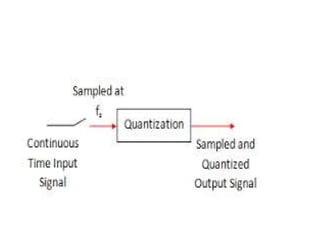
1. Quantization
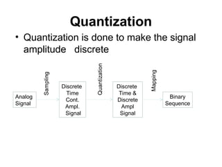
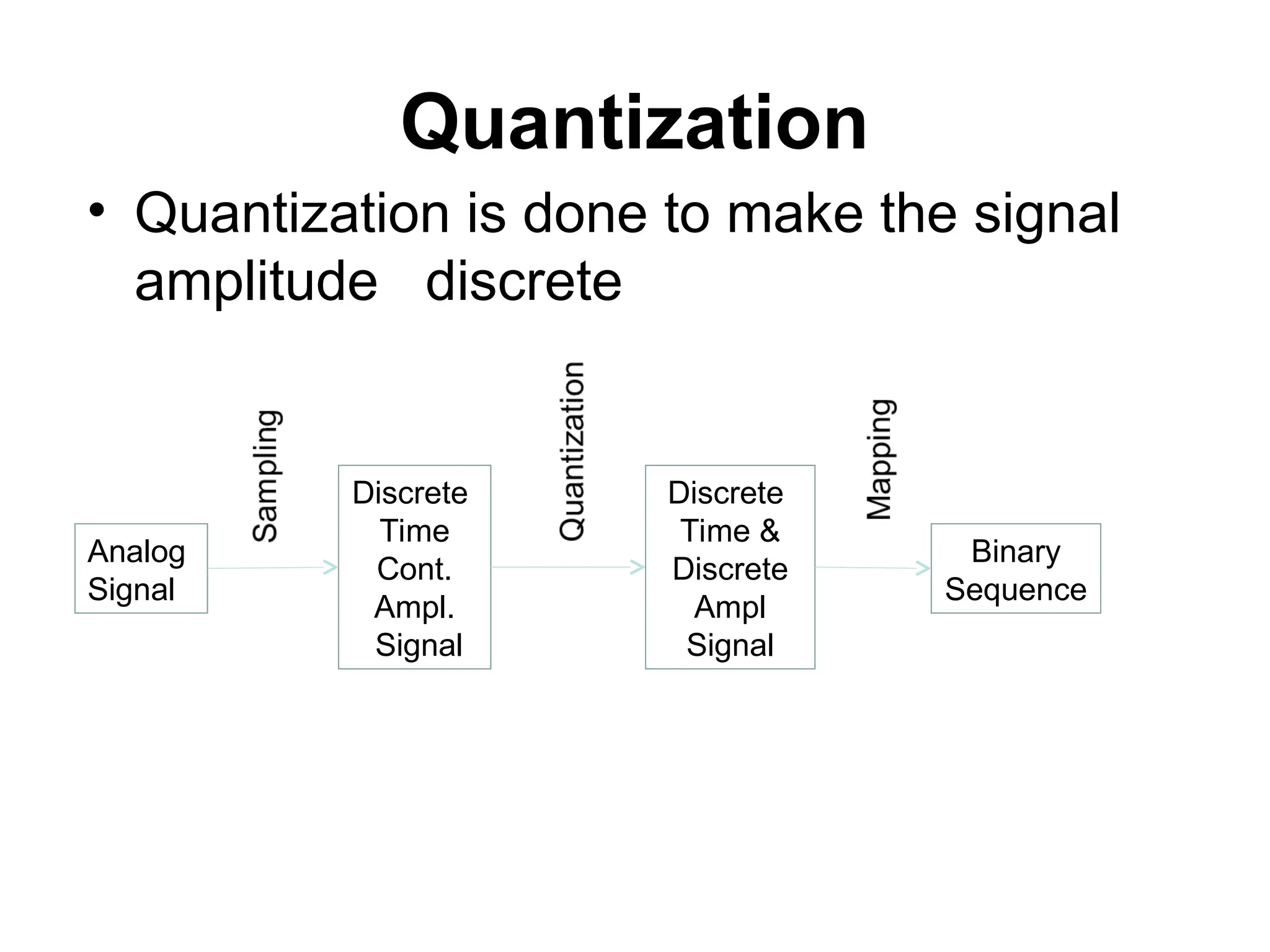
• Quantization is done to make the signal
amplitude discrete
Analog
Signal
Discrete
Time
Cont.
Ampl.
Signal
Discrete
Time &
Discrete
Ampl
Signal
Binary
Sequence

2. QUANTIZATION
• Definition : As the process of transformation of
a sample amplitude x[n] of message signal x(t)
at time t=nTs into a discrete amplitude v(nTs)
taken from a finite a set of prescribed values or
ampliyudes.
• Quantization converts a Discrete-Time Signal to
a Digital Signal.
• MATHEMATICAL REPRESENTATION:
xq[n] = Q( x[n] )

3. Quantization
Representing the analog sample’s value by a finite
set of levels is called quantizing.
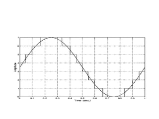
• Sampling results in a series of pulses of varying
amplitude values ranging between two limits:
a min and a max.
• The amplitude values are infinite between the two
limits.
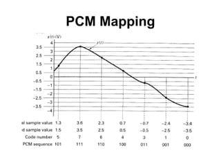
• We need to map the infinite amplitude values onto a
finite set of known values.
• This is achieved by dividing the distance between
min and max into Q levels, each of height Δ
Δ = (max min)/Q
‐

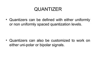
5. QUANTIZER
• Quantizers can be defined with either uniformly
or non uniformly spaced quantization levels.
• Quantizers can also be customized to work on
either uni-polar or bipolar signals.

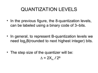
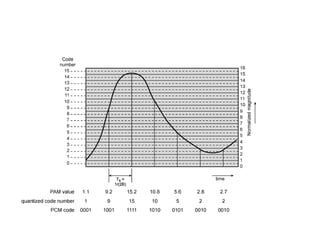
6. QUANTIZATION LEVELS
• In the previous figure, the 8-quantization levels,
can be labeled using a binary code of 3–bits.
• In general, to represent B-quantization levels we
need log2B(rounded to next highest integer) bits.
• The step size of the quantizer will be:
∆ = 2Xm / 2B

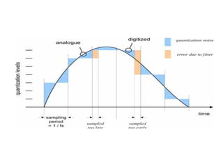
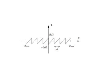
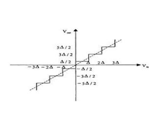
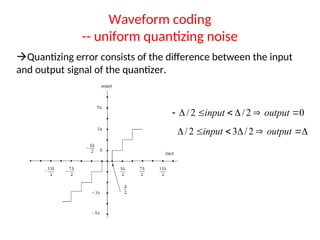
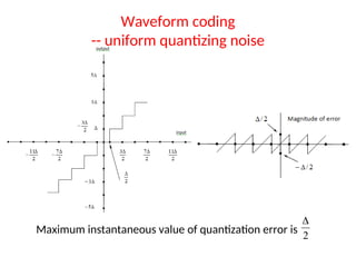
11. QUANTIZATION ERROR
• The quantized sample will generally differ from
the original signal. The difference between them
is called the quantization error.
e[n] = xq[n] - x[n]
• For a 3-bit Quantizer, if ∆/2 ≤ x[n] ≤ 3 ∆/2, then
xq[n] = ∆, and it follows that:
-∆/2 ≤ e[n] ≤ ∆/2

13. ADVANTAGES OF QUANTIZATION
• The quantized signal, which is an approximation
of the original signal, can be more efficiently
separated from ADDITIVE NOISE. (by using
repeaters).
• Transmission bandwidth can be controlled by
using an appropriate number of quantization
levels (and hence the bits to represent them).

16. PCM Mapping

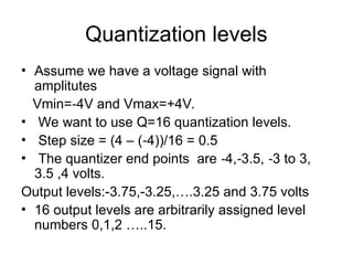
17. Quantization levels
• Assume we have a voltage signal with
amplitutes
Vmin= 4V and Vmax=+4V.
‐
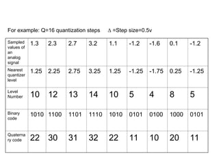
• We want to use Q=16 quantization levels.
• Step size = (4 – ( 4))/16 = 0.5
‐
• The quantizer end points are 4, 3.5, 3 to 3,
‐ ‐ ‐
3.5 ,4 volts.
Output levels:-3.75,-3.25,….3.25 and 3.75 volts
• 16 output levels are arbitrarily assigned level
numbers 0,1,2 …..15.

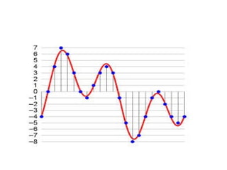
18. Sampled
values of
an
analog
signal
1.3 2.3 2.7 3.2 1.1 -1.2 -1.6 0.1 -1.2
Nearest
quantizer
level
1.25 2.25 2.75 3.25 1.25 -1.25 -1.75 0.25 -1.25
Level
Number 10 12 13 14 10 5 4 8 5
Binary
code
1010 1100 1101 1110 1010 0101 0100 1000 0101
Quaterna
ry code 22 30 31 32 22 11 10 20 11
For example: Q=16 quantization steps ∆ =Step size=0.5v

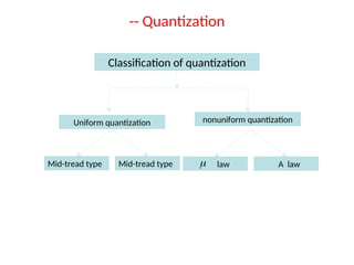
19. -- Quantization
Classification of quantization
Uniform quantization
Mid-tread type Mid-tread type
nonuniform quantization
law A law


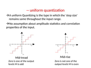
20. -- uniform quantization
A uniform Quantizing is the type in which the 'step size'
remains same throughout the input range.
No assumption about amplitude statistics and correlation
properties of the input.
Mid-tread
Zero is one of the output
levels M is odd
Mid-rise
Zero is not one of the
output levels M is even

21. Uniform Quantization

23. Quantizing error consists of the difference between the input
and output signal of the quantizer.
0
2
/
2
/ 





 output
input






 output
input 2
/
3
2
/
Waveform coding
-- uniform quantizing noise

24. Maximum instantaneous value of quantization error is 2

Waveform coding
-- uniform quantizing noise

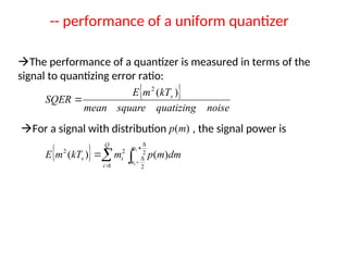
26. -- performance of a uniform quantizer
The performance of a quantizer is measured in terms of the
signal to quantizing error ratio:
 
noise
quatizing
square
mean
kT
m
E
SQER s )
(
2

For a signal with distribution , the signal power is
)
(m
p
   






Q
i
m
m
i
s
i
i
dm
m
p
m
kT
m
E
1
2
2
2
2
)
(
)
(

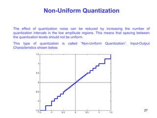
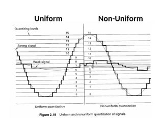
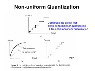
27. Non-Uniform Quantization
The effect of quantization noise can be reduced by increasing the number of
quantization intervals in the low amplitude regions. This means that spacing between
the quantization levels should not be uniform.
This type of quantization is called “Non-Uniform Quantization”. Input-Output
Characteristics shown below.
27

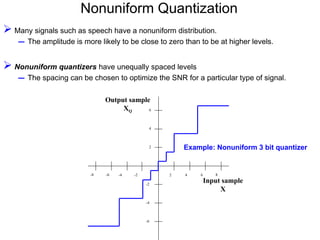
28. Nonuniform Quantization
 Many signals such as speech have a nonuniform distribution.
– The amplitude is more likely to be close to zero than to be at higher levels.
 Nonuniform quantizers have unequally spaced levels
– The spacing can be chosen to optimize the SNR for a particular type of signal.
2 4 6 8
2
4
6
-2
-4
-6
Input sample
X
Output sample
XQ
-2
-4
-6
-8
Example: Nonuniform 3 bit quantizer

29. Uniform and Nonuniform Quantization

30. Non-Uniform Quantization
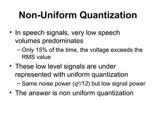
• In speech signals, very low speech
volumes predominates
– Only 15% of the time, the voltage exceeds the
RMS value
• These low level signals are under
represented with uniform quantization
– Same noise power (q2
/12) but low signal power
• The answer is non uniform quantization

31. Uniform Non-Uniform

32. Effect of Non-Linear Coding

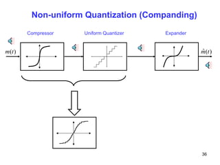
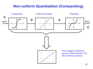
33. Non-uniform Quantization
Non-uniform quantization is achieved by, first passing the input signal
through a “compressor”. The output of the compressor is then passed
through a uniform quantizer.
The combined effect of the compressor and the uniform quantizer is that of
a non-uniform quantizer.
At the receiver the voice signal is restored to its original form by using an
expander.
This complete process of Compressing and Expanding the signal before
and after uniform quantization is called Companding.
33

34. -1
1
-1
x=m(t)/mp
1
y=g(x)
Non-uniform Quantization (Companding)
Input output relationship of a compressor. 34

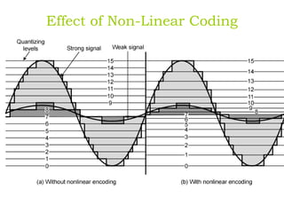
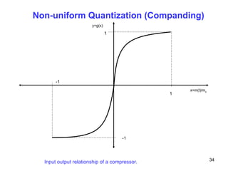
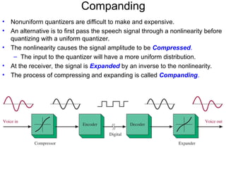
35. Companding
• Nonuniform quantizers are difficult to make and expensive.
• An alternative is to first pass the speech signal through a nonlinearity before
quantizing with a uniform quantizer.
• The nonlinearity causes the signal amplitude to be Compressed.
– The input to the quantizer will have a more uniform distribution.
• At the receiver, the signal is Expanded by an inverse to the nonlinearity.
• The process of compressing and expanding is called Companding.

36. Non-uniform Quantization (Companding)
Expander
)
(
ˆ t
m
Compressor
)
(t
m
Uniform Quantizer
36

37. Non-uniform Quantization (Companding)
)
(t
m
Expander
)
(
ˆ t
m
Compressor
)
(t
m
Uniform Quantizer
37
The 3 stages combine to
give the characteristics of a
Non-uniform quantizer.

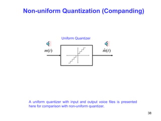
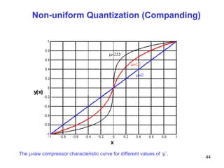
38. Non-uniform Quantization (Companding)
)
(t
m )
(
ˆ t
m
Uniform Quantizer
A uniform quantizer with input and output voice files is presented
here for comparison with non-uniform quantizer.
38

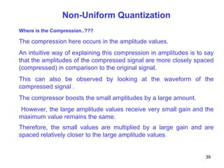
39. Non-Uniform Quantization
Where is the Compression..???
The compression here occurs in the amplitude values.
An intuitive way of explaining this compression in amplitudes is to say
that the amplitudes of the compressed signal are more closely spaced
(compressed) in comparison to the original signal.
This can also be observed by looking at the waveform of the
compressed signal .
The compressor boosts the small amplitudes by a large amount.
However, the large amplitude values receive very small gain and the
maximum value remains the same.
Therefore, the small values are multiplied by a large gain and are
spaced relatively closer to the large amplitude values.
39

40. Non-uniform Quantization
Compress the signal first
Then perform linear quantization
 Result in nonlinear quantization

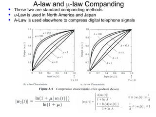
41. -Law Companding
• Telephones in the U.S., Canada
and Japan use -law
companding:
– Where  = 255 and |x(t)| < 1
ln(1 | ( )|)
| ( ) |
ln(1 )
x t
y t





0 1
1
Input |x(t)|
Output
|x(t)|

42. µ-law and A-law
Widely used compression algorithms

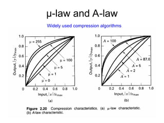
43. A-law and law Companding
• These two are standard companding methods.
• u-Law is used in North America and Japan
• A-Law is used elsewhere to compress digital telephone signals

44. Non-uniform Quantization (Companding)
The µ-law compressor characteristic curve for different values of ‘µ’.
44

45. Virtues & Limitation of PCM
The most important advantages of PCM are:
– Robustness to channel noise and
interference.
– Efficient regeneration of the coded signal
along the channel path.
– Efficient exchange between BT and SNR.
– Uniform format for different kind of base-
band signals.
– Flexible TDM.

46. Cont’d…
– Secure communication through the use of
special modulation schemes of encryption.
– These advantages are obtained at the cost of
more complexity and increased BT.
– With cost-effective implementations, the cost
issue no longer a problem of concern.
– With the availability of wide-band
communication channels and the use of
sophisticated data compression techniques, the
large bandwidth is not a serious problem.

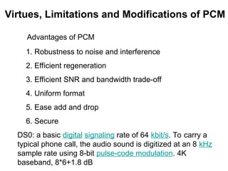
48. Advantages of PCM
1. Robustness to noise and interference
2. Efficient regeneration
3. Efficient SNR and bandwidth trade-off
4. Uniform format
5. Ease add and drop
6. Secure
DS0: a basic digital signaling rate of 64 kbit/s. To carry a
typical phone call, the audio sound is digitized at an 8 kHz
sample rate using 8-bit pulse-code modulation. 4K
baseband, 8*6+1.8 dB
Virtues, Limitations and Modifications of PCM