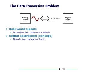
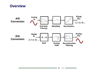
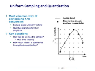
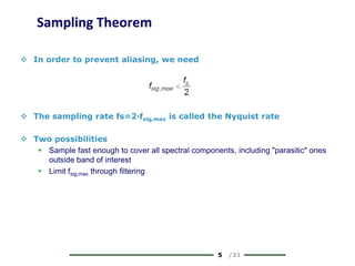
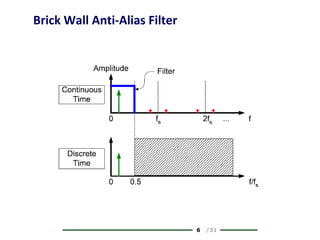
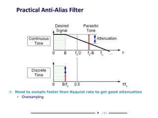
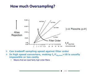
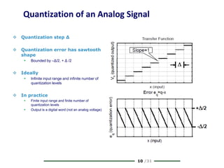
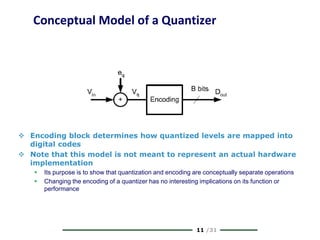
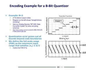
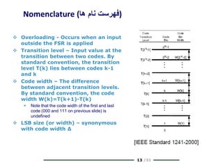
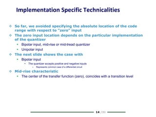
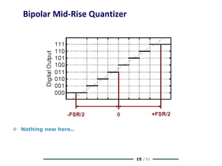
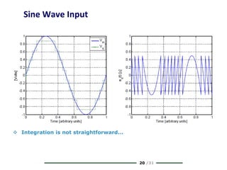
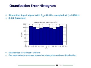
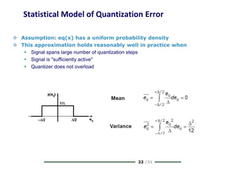
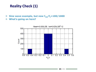
0 /31
Data Converter Basics
Dr. Hossein Shamsi
1 /31
Chapter 1
Sampling, Quantization, Reconstruction
2 /31
The Data Conversion Problem
 Real world signals
 Continuous time, continuous amplitude
 Digital abstraction (concept)
 Discrete time, discrete amplitude
3 /31
Overview
4 /31
Uniform Sampling and Quantization
 Most common way of
performing A/D
conversion
 Sample signal uniformly in time
 Quantize signal uniformly in
amplitude
 Key questions
 How fast do we need to sample?
• Must avoid "aliasing“
 How much "noise" is added due
to amplitude quantization?
5 /31
Sampling Theorem
 In order to prevent aliasing, we need
 The sampling rate fs=2·fsig,max is called the Nyquist rate
 Two possibilities
 Sample fast enough to cover all spectral components, including "parasitic" ones
outside band of interest
 Limit fsig,max through filtering
6 /31
Brick Wall Anti-Alias Filter
7 /31
Practical Anti-Alias Filter
 Need to sample faster than Nyquist rate to get good attenuation
 Oversampling
8 /31
How much Oversampling?
 Can tradeoff sampling speed against filter order
 In high speed converters, making fs/fsig,max>10 is usually
impossible or too costly
 Means that we need fairly high order filters
9 /31
Classes of Sampling
 Nyquist-rate sampling (fs > 2·fsig,max)
 Nyquist data converters
 In practice always slightly oversampled
 Oversampling (fs >> 2·fsig,max)
 Oversampled data converters
 Anti-alias filtering is often trivial
 Oversampling also helps reduce "quantization noise"
 More later
 Undersampling, subsampling (fs < 2·fsig,max)
 Exploit aliasing to mix RF/IF signals down to baseband
10 /31
Quantization of an Analog Signal
 Quantization step Δ
 Quantization error has sawtooth
shape
 Bounded by –Δ/2, + Δ /2
 Ideally
 Infinite input range and infinite number of
quantization levels
 In practice
 Finite input range and finite number of
quantization levels
 Output is a digital word (not an analog voltage)
11 /31
Conceptual Model of a Quantizer
 Encoding block determines how quantized levels are mapped into
digital codes
 Note that this model is not meant to represent an actual hardware
implementation
 Its purpose is to show that quantization and encoding are conceptually separate operations
 Changing the encoding of a quantizer has no interesting implications on its function or
performance
12 /31
Encoding Example for a B-Bit Quantizer
 Example: B=3
 23=8 distinct output codes
 Diagram on the left shows "straight-binary
encoding“
 See e.g. Analog Devices "MT-009: Data
Converter Codes" for other encoding
schemes
 http://www.analog.com/en/content/0,2886,760%255
F788%255F91285,000
 Quantization error grows out of
bounds beyond code boundaries
 We define the full scale range
(FSR) as the maximum input
range that satisfies |eq| ≤ Δ/2
 Implies that FSR=2B·Δ
13 /31
Nomenclature (‫ها‬ ‫نام‬ ‫)فهرست‬
 Overloading - Occurs when an input
outside the FSR is applied
 Transition level – Input value at the
transition between two codes. By
standard convention, the transition
level T(k) lies between codes k-1
and k
 Code width – The difference
between adjacent transition levels.
By standard convention, the code
width W(k)=T(k+1)-T(k)
 Note that the code width of the first and last
code (000 and 111 on previous slide) is
undefined
 LSB size (or width) – synonymous
with code width Δ
14 /31
Implementation Specific Technicalities
 So far, we avoided specifying the absolute location of the code
range with respect to "zero" input
 The zero input location depends on the particular implementation
of the quantizer
 Bipolar input, mid-rise or mid-tread quantizer
 Unipolar input
 The next slide shows the case with
 Bipolar input
• The quantizer accepts positive and negative inputs
– Represents common case of a differential circuit
 Mid-rise characteristic
 The center of the transfer function (zero), coincides with a transition level
15 /31
Bipolar Mid-Rise Quantizer
 Nothing new here..
16 /31
Bipolar Mid-Tread Quantizer
 In theory, less sensitive to small disturbance around zero
 In practice, offsets larger than Δ/2 (due to device mismatch) often make this argument irrelevant
 Asymmetric full-scale range, unless we use odd number of codes
17 /31
Unipolar Quantizer
 Usually define origin where first code and straight line fit intersect
 Otherwise, there would be a systematic offset
 Usable range is reduced by Δ/2 below zero
18 /31
Effect of Quantization Error on Signal
 Two aspects
 How much noise power does quantization add to samples?
 How is this noise power distributed in frequency?
 Quantization error is a deterministic function of the signal
 Should be able answer above questions using a deterministic analysis
 But, unfortunately, such an analysis strongly depends on the chosen signal and
can be very complex
 Strategy
 Build basic intuition using simple deterministic signals
 Next, abandon idea of deterministic representation and revert to a "general"
statistical model (to be used with caution!)
19 /31
Ramp Input
 Applying a ramp signal (periodic sawtooth) at the input of the
quantizer gives the following time domain waveform for eq
 What is the average power of this waveform?
 Integrate over one period
20 /31
Sine Wave Input
 Integration is not straightforward...
21 /31
Quantization Error Histogram
 Sinusoidal input signal with fsig=101Hz, sampled at fs=1000Hz
 8-bit Quantizer
 Distribution is "almost" uniform
 Can approximate average power by integrating uniform distribution
22 /31
Statistical Model of Quantization Error
 Assumption: eq(x) has a uniform probability density
 This approximation holds reasonably well in practice when
 Signal spans large number of quantization steps
 Signal is "sufficiently active"
 Quantizer does not overload
23 /31
Reality Check (1)
 Sine wave example, but now fsig/fs=100/1000
 What's going on here?
24 /31
Analysis (1)
 Sampled signal is repetitive and has only a few distinct values
 This also means that the Quantizer generates only a few distinct values of eq; not a uniform
distribution
25 /31
Analysis (2)
 Signal repeats every m samples, where m is the smallest integer
that satisfies
 This means that eq(n) has at best 10 distinct values, even if we take
many more samples
26 /31
Signal-to-Quantization-Noise Ratio
 Assuming uniform distribution of eq and a full-scale sinusoidal
input, we have
– 27 –
SNR Versus Vin
– 28 –
Example #1
29 /31
Quantization Noise Spectrum (1)
 How is the quantization noise power distributed in frequency?
 First think about applying a sine wave to a quantizer, without sampling (output is
continuous time)
 Quantization results in an "infinite" number of harmonics
30 /31
Quantization Noise Spectrum (2)
 Now sample the signal at the output
 All harmonics (an "infinite" number of them) will alias into band from 0 to fs/2
 Quantization noise spectrum becomes "white”
 Interchanging sampling and quantization won’t change this
situation results in an "infinite" number of harmonics
31 /31
Quantization Noise Spectrum (3)
 Can show that the quantization noise power is indeed distributed
(approximately) uniformly in frequency
 Again, this is provided that the quantization error is "sufficiently random"
“one-sided spectrum”

slide1-1.ppt

  • 1.
    0 /31 Data ConverterBasics Dr. Hossein Shamsi
  • 2.
    1 /31 Chapter 1 Sampling,Quantization, Reconstruction
  • 3.
    2 /31 The DataConversion Problem  Real world signals  Continuous time, continuous amplitude  Digital abstraction (concept)  Discrete time, discrete amplitude
  • 4.
  • 5.
    4 /31 Uniform Samplingand Quantization  Most common way of performing A/D conversion  Sample signal uniformly in time  Quantize signal uniformly in amplitude  Key questions  How fast do we need to sample? • Must avoid "aliasing“  How much "noise" is added due to amplitude quantization?
  • 6.
    5 /31 Sampling Theorem In order to prevent aliasing, we need  The sampling rate fs=2·fsig,max is called the Nyquist rate  Two possibilities  Sample fast enough to cover all spectral components, including "parasitic" ones outside band of interest  Limit fsig,max through filtering
  • 7.
    6 /31 Brick WallAnti-Alias Filter
  • 8.
    7 /31 Practical Anti-AliasFilter  Need to sample faster than Nyquist rate to get good attenuation  Oversampling
  • 9.
    8 /31 How muchOversampling?  Can tradeoff sampling speed against filter order  In high speed converters, making fs/fsig,max>10 is usually impossible or too costly  Means that we need fairly high order filters
  • 10.
    9 /31 Classes ofSampling  Nyquist-rate sampling (fs > 2·fsig,max)  Nyquist data converters  In practice always slightly oversampled  Oversampling (fs >> 2·fsig,max)  Oversampled data converters  Anti-alias filtering is often trivial  Oversampling also helps reduce "quantization noise"  More later  Undersampling, subsampling (fs < 2·fsig,max)  Exploit aliasing to mix RF/IF signals down to baseband
  • 11.
    10 /31 Quantization ofan Analog Signal  Quantization step Δ  Quantization error has sawtooth shape  Bounded by –Δ/2, + Δ /2  Ideally  Infinite input range and infinite number of quantization levels  In practice  Finite input range and finite number of quantization levels  Output is a digital word (not an analog voltage)
  • 12.
    11 /31 Conceptual Modelof a Quantizer  Encoding block determines how quantized levels are mapped into digital codes  Note that this model is not meant to represent an actual hardware implementation  Its purpose is to show that quantization and encoding are conceptually separate operations  Changing the encoding of a quantizer has no interesting implications on its function or performance
  • 13.
    12 /31 Encoding Examplefor a B-Bit Quantizer  Example: B=3  23=8 distinct output codes  Diagram on the left shows "straight-binary encoding“  See e.g. Analog Devices "MT-009: Data Converter Codes" for other encoding schemes  http://www.analog.com/en/content/0,2886,760%255 F788%255F91285,000  Quantization error grows out of bounds beyond code boundaries  We define the full scale range (FSR) as the maximum input range that satisfies |eq| ≤ Δ/2  Implies that FSR=2B·Δ
  • 14.
    13 /31 Nomenclature (‫ها‬‫نام‬ ‫)فهرست‬  Overloading - Occurs when an input outside the FSR is applied  Transition level – Input value at the transition between two codes. By standard convention, the transition level T(k) lies between codes k-1 and k  Code width – The difference between adjacent transition levels. By standard convention, the code width W(k)=T(k+1)-T(k)  Note that the code width of the first and last code (000 and 111 on previous slide) is undefined  LSB size (or width) – synonymous with code width Δ
  • 15.
    14 /31 Implementation SpecificTechnicalities  So far, we avoided specifying the absolute location of the code range with respect to "zero" input  The zero input location depends on the particular implementation of the quantizer  Bipolar input, mid-rise or mid-tread quantizer  Unipolar input  The next slide shows the case with  Bipolar input • The quantizer accepts positive and negative inputs – Represents common case of a differential circuit  Mid-rise characteristic  The center of the transfer function (zero), coincides with a transition level
  • 16.
    15 /31 Bipolar Mid-RiseQuantizer  Nothing new here..
  • 17.
    16 /31 Bipolar Mid-TreadQuantizer  In theory, less sensitive to small disturbance around zero  In practice, offsets larger than Δ/2 (due to device mismatch) often make this argument irrelevant  Asymmetric full-scale range, unless we use odd number of codes
  • 18.
    17 /31 Unipolar Quantizer Usually define origin where first code and straight line fit intersect  Otherwise, there would be a systematic offset  Usable range is reduced by Δ/2 below zero
  • 19.
    18 /31 Effect ofQuantization Error on Signal  Two aspects  How much noise power does quantization add to samples?  How is this noise power distributed in frequency?  Quantization error is a deterministic function of the signal  Should be able answer above questions using a deterministic analysis  But, unfortunately, such an analysis strongly depends on the chosen signal and can be very complex  Strategy  Build basic intuition using simple deterministic signals  Next, abandon idea of deterministic representation and revert to a "general" statistical model (to be used with caution!)
  • 20.
    19 /31 Ramp Input Applying a ramp signal (periodic sawtooth) at the input of the quantizer gives the following time domain waveform for eq  What is the average power of this waveform?  Integrate over one period
  • 21.
    20 /31 Sine WaveInput  Integration is not straightforward...
  • 22.
    21 /31 Quantization ErrorHistogram  Sinusoidal input signal with fsig=101Hz, sampled at fs=1000Hz  8-bit Quantizer  Distribution is "almost" uniform  Can approximate average power by integrating uniform distribution
  • 23.
    22 /31 Statistical Modelof Quantization Error  Assumption: eq(x) has a uniform probability density  This approximation holds reasonably well in practice when  Signal spans large number of quantization steps  Signal is "sufficiently active"  Quantizer does not overload
  • 24.
    23 /31 Reality Check(1)  Sine wave example, but now fsig/fs=100/1000  What's going on here?
  • 25.
    24 /31 Analysis (1) Sampled signal is repetitive and has only a few distinct values  This also means that the Quantizer generates only a few distinct values of eq; not a uniform distribution
  • 26.
    25 /31 Analysis (2) Signal repeats every m samples, where m is the smallest integer that satisfies  This means that eq(n) has at best 10 distinct values, even if we take many more samples
  • 27.
    26 /31 Signal-to-Quantization-Noise Ratio Assuming uniform distribution of eq and a full-scale sinusoidal input, we have
  • 28.
    – 27 – SNRVersus Vin
  • 29.
  • 30.
    29 /31 Quantization NoiseSpectrum (1)  How is the quantization noise power distributed in frequency?  First think about applying a sine wave to a quantizer, without sampling (output is continuous time)  Quantization results in an "infinite" number of harmonics
  • 31.
    30 /31 Quantization NoiseSpectrum (2)  Now sample the signal at the output  All harmonics (an "infinite" number of them) will alias into band from 0 to fs/2  Quantization noise spectrum becomes "white”  Interchanging sampling and quantization won’t change this situation results in an "infinite" number of harmonics
  • 32.
    31 /31 Quantization NoiseSpectrum (3)  Can show that the quantization noise power is indeed distributed (approximately) uniformly in frequency  Again, this is provided that the quantization error is "sufficiently random" “one-sided spectrum”