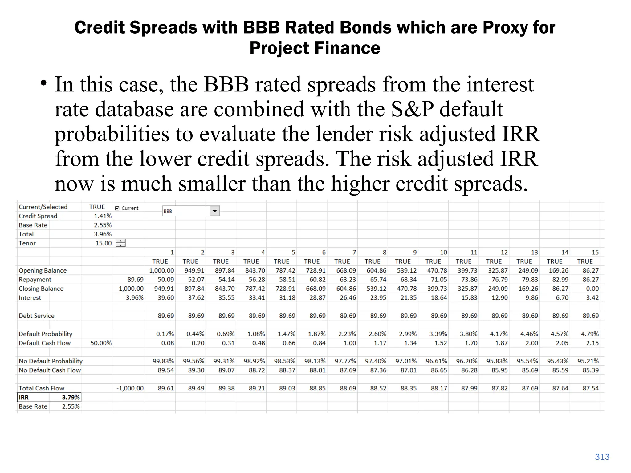
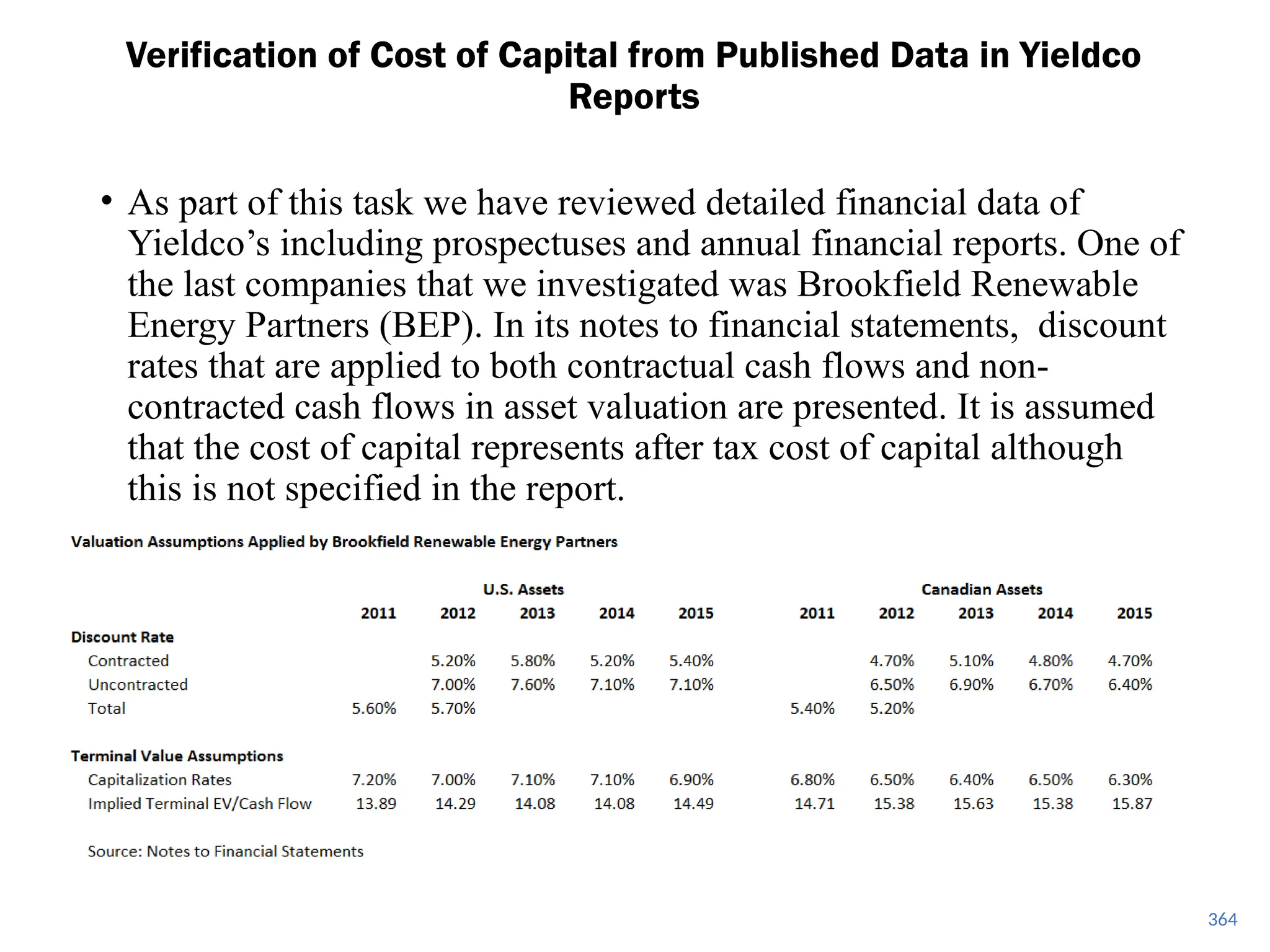
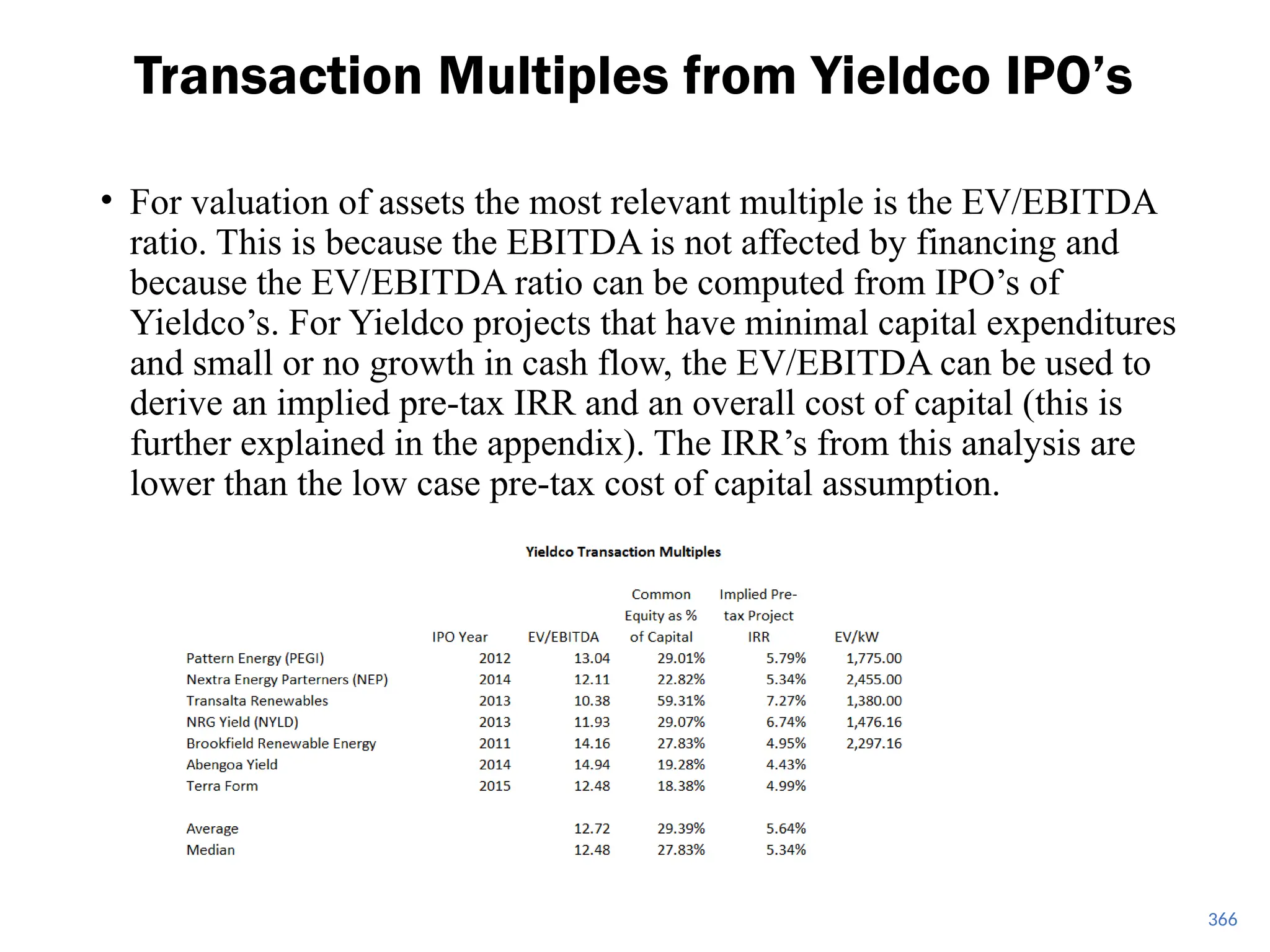
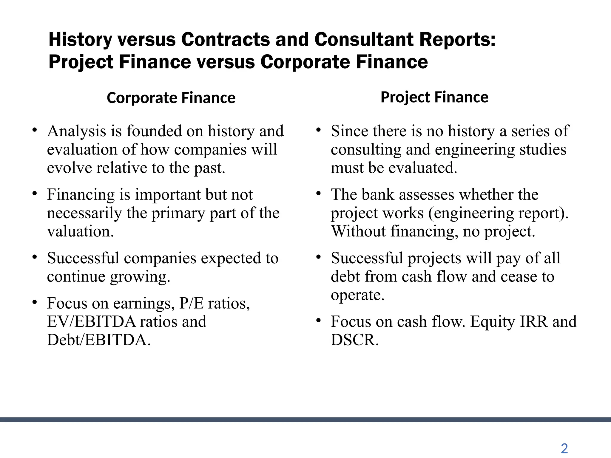
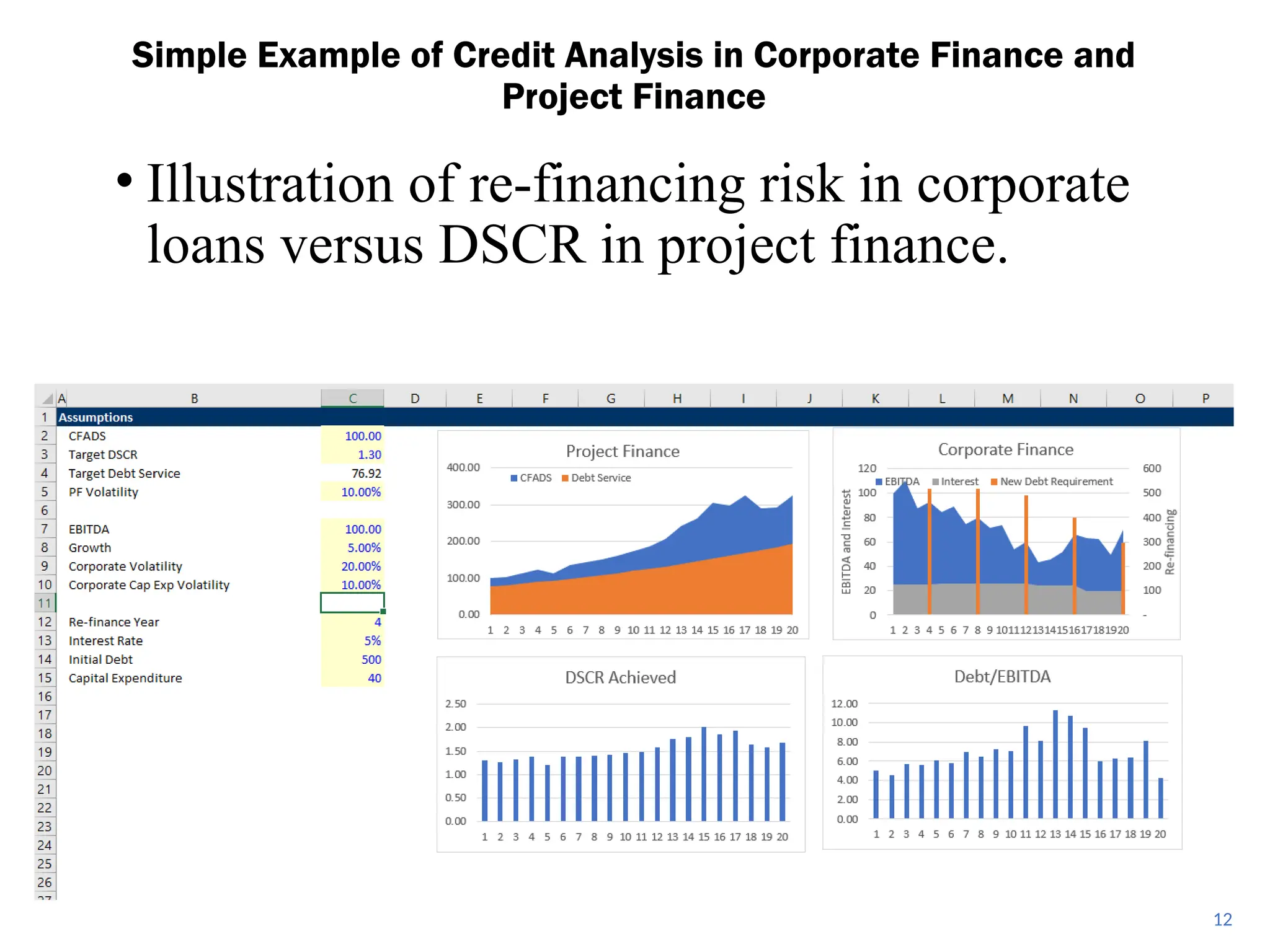
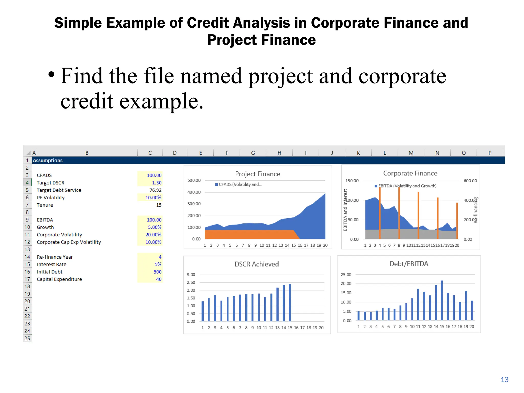
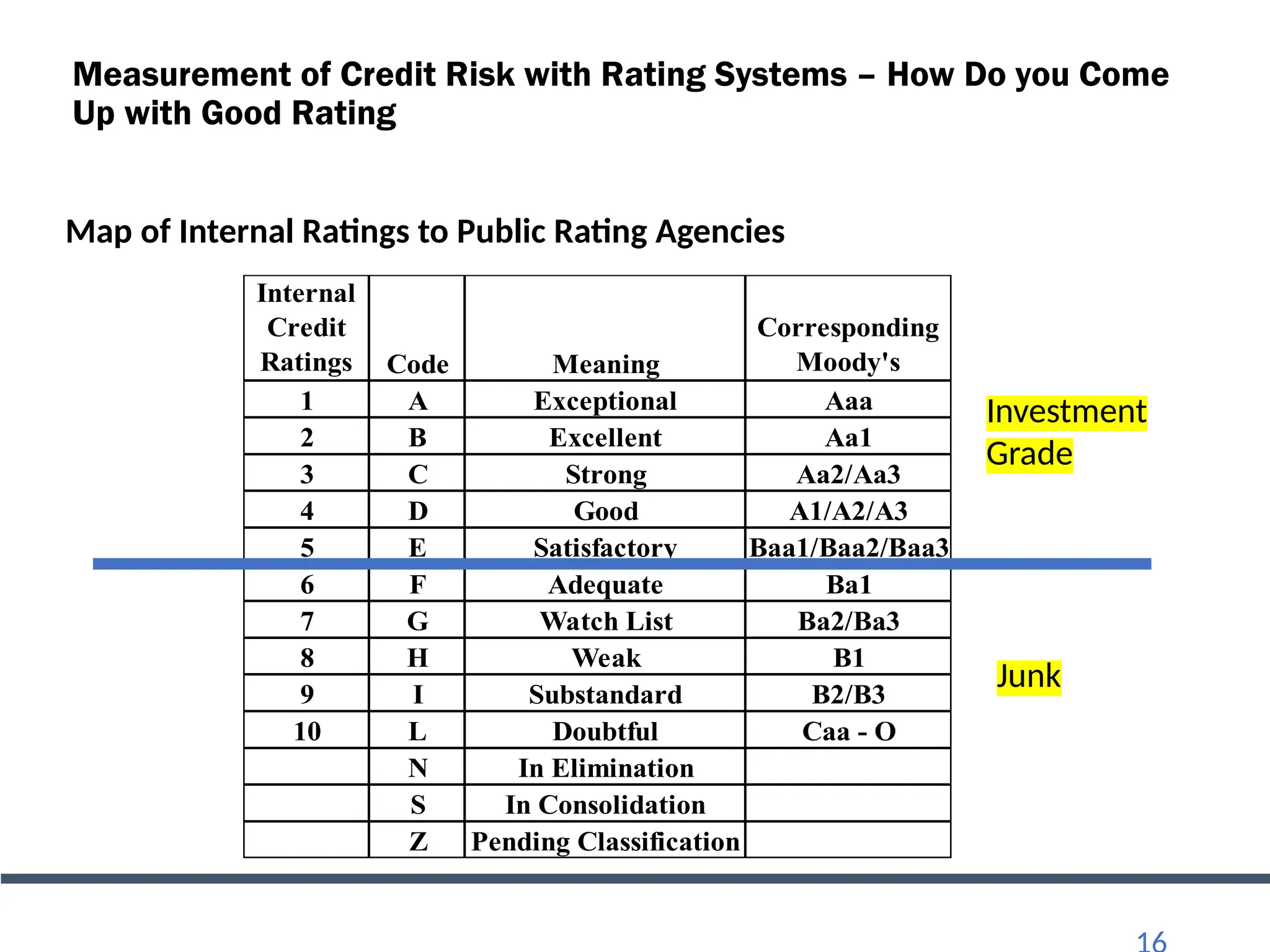
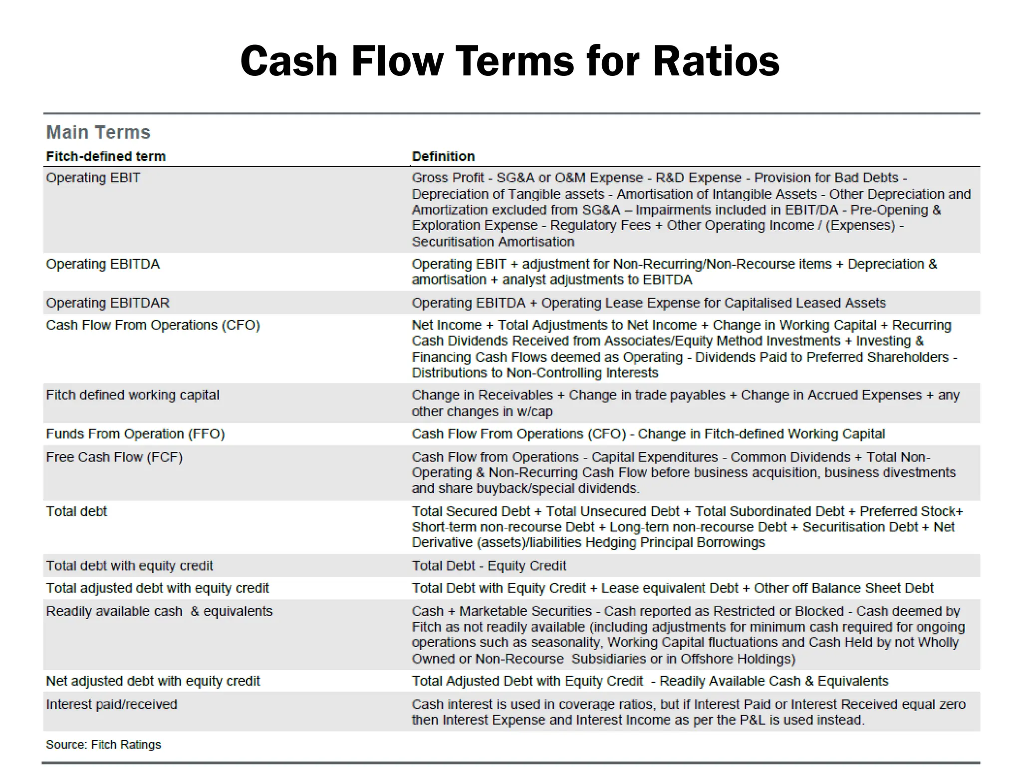
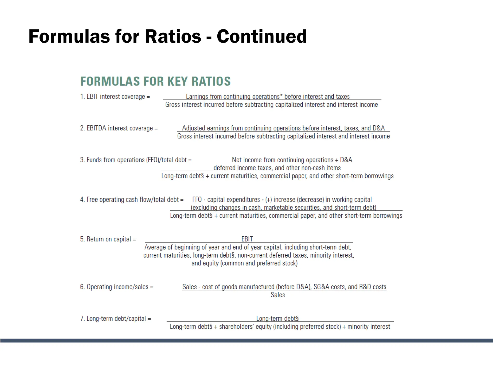
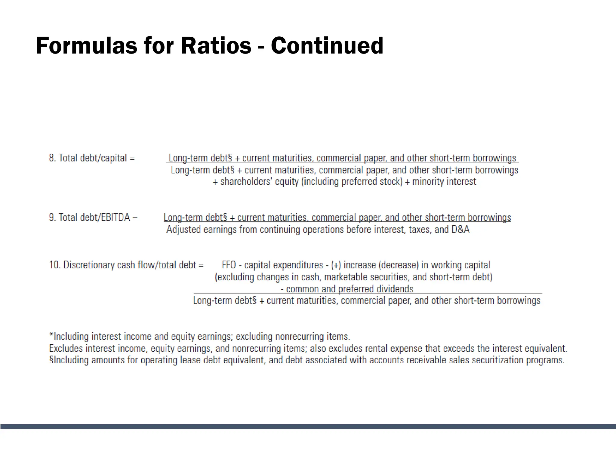
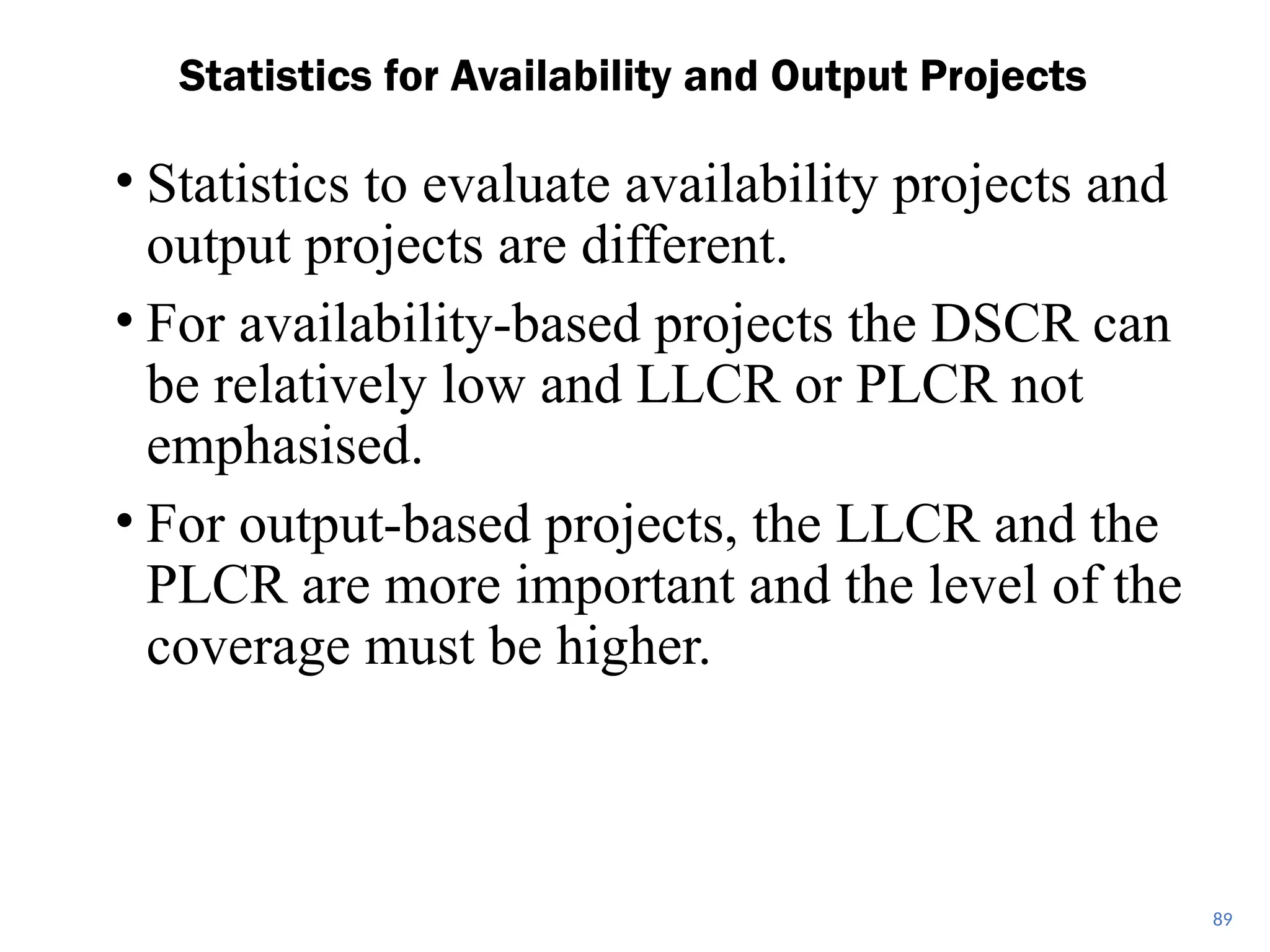
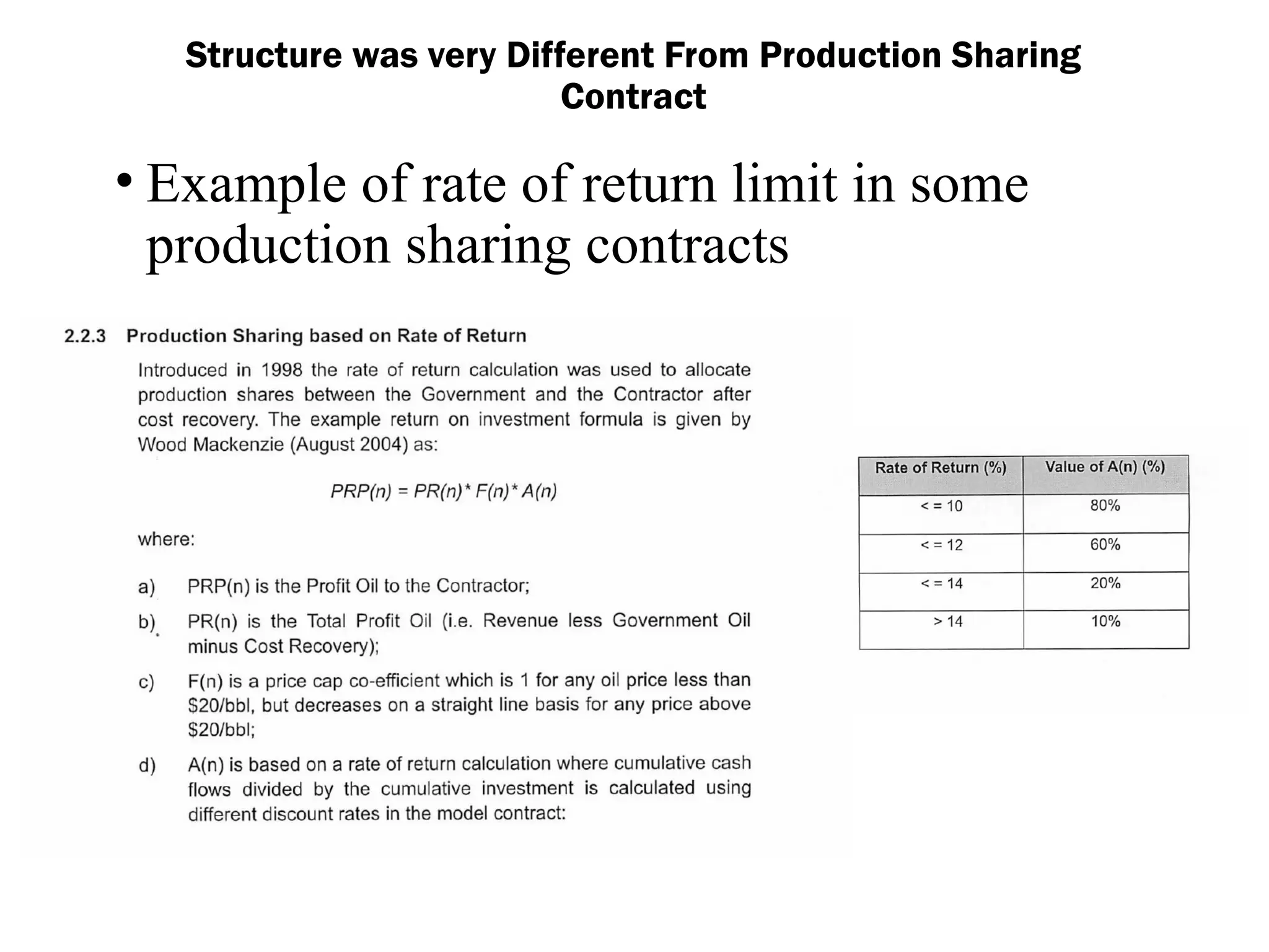
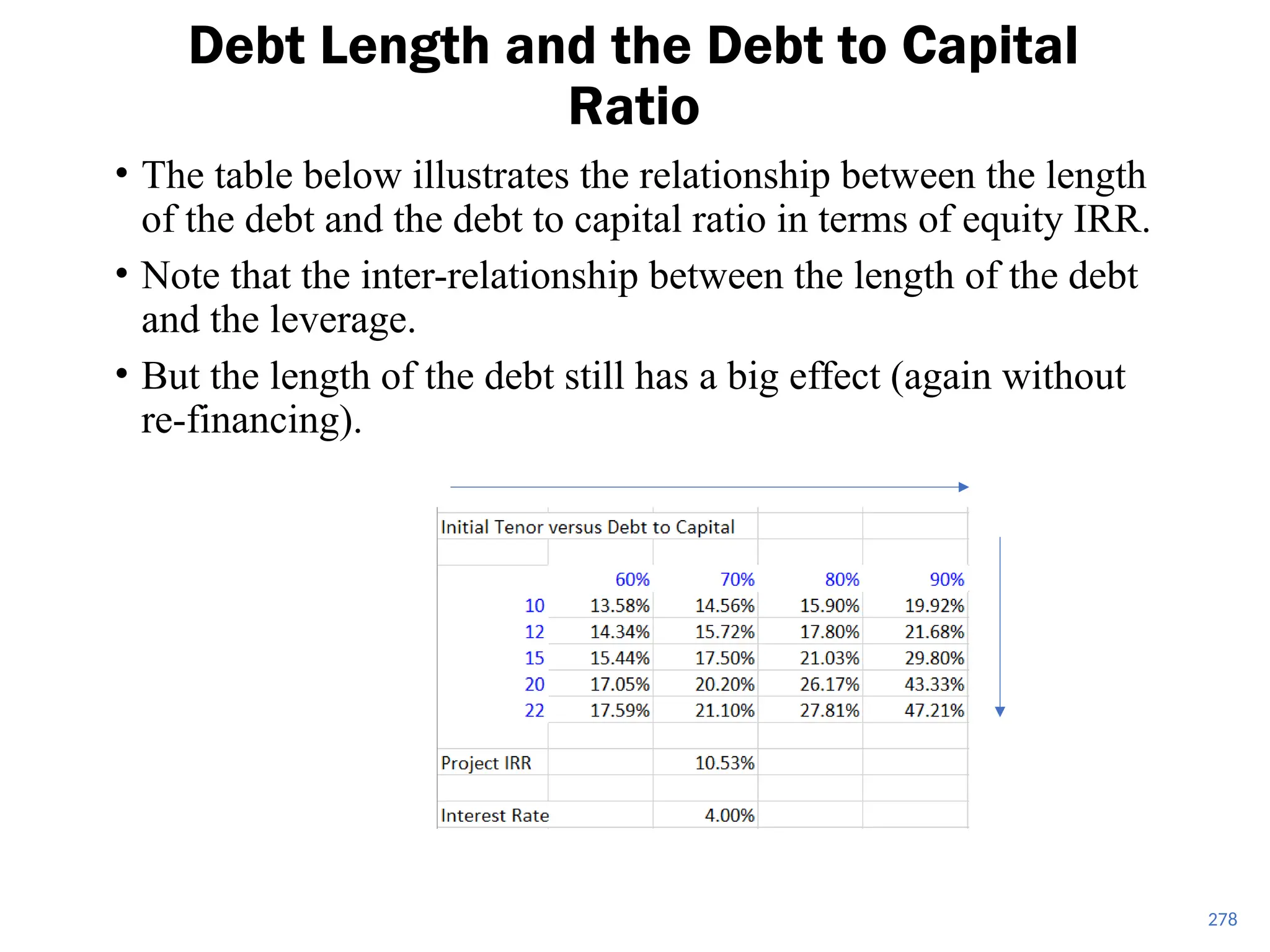
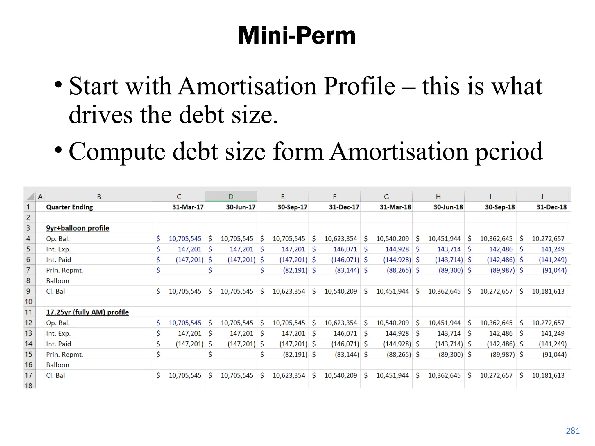
The document compares project finance and corporate finance, highlighting their distinct approaches to valuation and risk assessment, with project finance relying heavily on forecasts and cash flow metrics while corporate finance is grounded in historical company performance. It discusses key financial metrics such as Debt Service Coverage Ratio (DSCR), equity Internal Rate of Return (IRR), and other valuation ratios, emphasizing the importance of these measures in project finance for determining debt sizing and repayment structures. Additional sections detail the contractual nuances in project finance, variations in risk assessment across industries, and the interplay of different financial ratios in assessing credit risk.

1. Project Finance Lecture

2. History versus Contracts and Consultant Reports:
Project Finance versus Corporate Finance
Corporate Finance
• Analysis is founded on history and
evaluation of how companies will
evolve relative to the past.
• Financing is important but not
necessarily the primary part of the
valuation.
• Successful companies expected to
continue growing.
• Focus on earnings, P/E ratios,
EV/EBITDA ratios and
Debt/EBITDA.
Project Finance
• Since there is no history a series of
consulting and engineering studies
must be evaluated.
• The bank assesses whether the
project works (engineering report).
Without financing, no project.
• Successful projects will pay of all
debt from cash flow and cease to
operate.
• Focus on cash flow. Equity IRR and
DSCR.
2

3. • Solar case language:
• Notwithstanding any other provision of the Financing Documents,
there shall be no recourse against the stockholders … for any liability
to the Lenders in connection with any breach or default under this
Agreement
• Notwithstanding the foregoing, nothing contained in this Article
• (i) Borrower shall remain fully liable to the extent that be liable
for its own actions with respect to, any fraud, willful misconduct
or gross negligence,
• (ii) limit in any respect the enforceability against an Acceptable
O&M Reserve Letter of Credit, an Acceptable Major Maintenance
Reserve Letter of Credit, an Acceptable DSR Letter of Credit
• (iii) release any legal consultant in its capacity as such from
liability on account of any legal opinion rendered in connection
with the transactions contemplated hereby.
Project Finance and Non-Recourse Debt
3

4. City is Like a Corporation/Project is Business
4
Individual
Business or
Family is like
project Finance

5. Family is Like Corporation, Person is Like Project Finance
5
Person is the
project
Entire Family
is the
Corporation

6. Time-Line is Crucial in Project Finance
Sponsor
Risk
Time
Letter
of
Intent
Fuel Supply
and Power
Purchase
Agreements
Financial
Agreements
Signed
Ground-
breaking
Commissioning
Steady-State
Operation
Technical
and
Economic
Feasibility
Project
Identi-
fication
Permits
Obtained
Financial
Structure
Negotiated
Construction
Time to Complete Task (months)
2 6 12 20 24 48 49
8
Completion
Test
Financial
Close
A crucial Feature of Project
finance is CHANGING --
DECLINING RISK
RISK

7. • On the Term Conversion Date, Borrower may
convert a portion of the Construction Loans,
as set forth below, into Term Loans
• Availability. Each Lender agrees to advance
to Borrower from time to time during the
applicable Construction Loan Availability
Period, but no more frequently than once per
month, a “Construction Loan”
• Availability from Financial Close, to COD
Periods in Solar Case
7

8. Project Finance Model Structure Changes at COD
Development is Dating
period. Probability of
failure is high
FC is just after
engagement
date
Pay your Bills and re-structure
your life. Stuck with PPA type
contract. May default.
Commitment
Fee
Decommissioning
Date
Father of the
bride makes
commitment
to pay for
wedding
Pay for Wedding
with Other peoples
money
After COD, cash flow is
presented in the cash
flow waterfall and the
last line is dividends
Before COD, cash flow
is presented in the
sources and uses
statement
COD is
Wedding
Date

9. Why Ratios are Different in Project Finance
and Corporate Finance
• Continuing Large Capital Expenditures in Corporate
Finance
• Large Bullet Repayments in Corporate Finance that Do
Not Correspond to Cash Flow
• No Customizing Repayments to Cash Flow
• In Corporate Finance, Source of Repayment in Re-
Financing

10. Difference Between Ratios for Project Finance and
Corporate Finance
Corporate Finance Project Finance
• Debt Service Buffer
• DSCR
• LLCR
• PLCR
• Skin in the Game
• Debt to Capital
• Debt to Equity
10
• Interest Coverage Buffer
• EBITDA/Interest
• EBIT/Interest
• FFO/Interest
• Time To Repay Debt
• Debt/EBITDA
• Debt/FFO or FFO/Debt
• Value of Company to Debt
• Debt to Equity
• Debt to Capital

11. • Project Finance Investment
• Equity IRR
• Project IRR
• Equity NPV
• Project NPV
• Project Finance Debt
• DSCR
• LLCR
• PLCR
• Liquidity
• Debt Service Reserve
Valuation Metrics in Project Finance and
Corporate Finance
• Corporate Finance Valuation
•P/E Ratio
•EV/EBITDA
•Projected Dividend and Earnings
•Free Cash Flow
• Corporate Finance Debt
•Times Interest Earned
•Debt to EBITDA
•Debt to Capital
• Corporate Finance Liquidity
•Current Ratio; Quick Ratio

12. • Illustration of re-financing risk in corporate
loans versus DSCR in project finance.
Simple Example of Credit Analysis in Corporate Finance and
Project Finance
12

13. • Find the file named project and corporate
credit example.
Simple Example of Credit Analysis in Corporate Finance and
Project Finance
13

14. • Cases and Project Finance versus Corporate Finance
• Solar or Wind Farm
• Airport or Seaport
• Real Estate
• Hotel
• Mixed Development
• Multi-Family
• Construction Projects
• Others
• Hospital/School
• Toll Road
• Factory
• Oil Field
Three Different Cases
14

15. Airport Case and Project Finance Definition
15

16. Measurement of Credit Risk with Rating Systems – How Do you Come
Up with Good Rating
Internal
Credit
Ratings Code Meaning
Corresponding
Moody's
1 A Exceptional Aaa
2 B Excellent Aa1
3 C Strong Aa2/Aa3
4 D Good A1/A2/A3
5 E Satisfactory Baa1/Baa2/Baa3
6 F Adequate Ba1
7 G Watch List Ba2/Ba3
8 H Weak B1
9 I Substandard B2/B3
10 L Doubtful Caa - O
N In Elimination
S In Consolidation
Z Pending Classification
Map of Internal Ratings to Public Rating Agencies
Investment
Grade
Junk

17. Project Finance ties to BBB- (Baa3)
Investment Grade Junk

18. Part 2: Bank Perspective in Project Finance:
Risk Analysis and Structuring with DSCR,
LLCR and PLCR

19. • The DSCR is computed from prospective cash
flow like other ratios in project finance including
the project IRR, equity IRR and other ratios.
• There could be many definitions of the DSCR,
but the general definition is CFADS/DS where:
• CFADS is cash flow available for debt service
• DS includes interest expense, debt repayment and
fees
• The DSCR can be explained with the graph of
CFADS and Debt Service
DSCR Key Points

20. • The key point about the DSCR is that it is a
measure of break-even from a forecasted cash
flow. For example if the cash flow is 150 and
the debt service is 100, the DSCR is 1.5. In this
case the cash flow can go down by 50 before a
default occurs. So in percentage terms this
means that a reduction of 50/150 or 33%.
• In terms of a formula, the percent reduction
before default can be expressed using the
formula:
• Percent reduction = (DSCR-1)/DSCR
DSCR as a Buffer to Break Even
20

21. • The DSCR has at least two different uses in
project finance.
• One use is for determining the size of the debt. This
means that if the projected DSCR is below a certain
level, the loan should not be made. For example, if
the DSCR is below 1.35, then the amount of debt
must be reduced.
• A second is for dividend covenants (a lower level,
say 1.1). This means if the DSCR falls below a
certain level, then dividends are not allowed to be
paid. If dividends are not allow (a dividend trap),
then the cash that could have been paid in dividends
is put in a reserve account.
DSCR for Target Debt Size and Covenants
21

22. • DSCR is a measure of the chance of default.
When the DSCR is 1.0 or below, there is not
enough cash to pay the debt service.
• This means the probability of the DSCR falling
to 1.0 is similar to the probability of default.
• If the DSCR falls to 1.0 or below in any single
period, a default has occurred in the period.
This is why the minimum DSCR rather than the
average DSCR is used in discussing
transactions.
DSCR is Minimum over Debt Tenure
22

23. • DSCR is used in project finance because the
debt service and in particular the repayments
are structured according to expected cash
flow.
• In corporate finance on the other hand, there
may be bonds with bullet repayments where
the ability to re-finance defines the credit
risk. With bullet repayments, the DSCR
would fluctuate.
• You can explain this with a diagram.
Why DSCR is Used in Project Finance and Less in Corporate
Finance
23

24. • Wind Study with different probability levels (the
FPL Case)
• Solar case with probability levels
• No dividends allowed if the Average Annual Debt
Service Coverage Ratio calculated as of the
Repayment Date immediately preceding such
Distribution Date is less than 1.20 to 1.00
• Permit the Average Annual Debt Service
Coverage Ratio as of the last day of any Quarterly
Date commencing from the first Repayment Date
to be less than 1.10 to 1.00 or
DSCR Case Study and Exercise
24

25. Distributions
• Make any distribution unless such distribution is made from Distributable Cash and on a Distribution
Date; if the Average Annual DSCR calculated as of the Repayment Date immediately preceding such
Distribution Date is less than 1.20 to 1.00, or
• the Average Annual Projected DSCR (based upon the Term Conversion Date Base Case Projections
but updated for actual operating performance of the Project through the applicable Repayment Date)
calculated as of the Repayment Date immediately preceding such Distribution Date, is less than 1.20
to 1.00;
Financial Covenants (Default)
• Permit the Average Annual DSCR as of the last day of any Quarterly Date commencing
from the first Repayment Date to be less than 1.10 to 1.00 or
• Permit the Average Annual Projected DSCR (based upon the Term Conversion Date Base
Case Projections but updated for actual operating performance of the Project through the
applicable Repayment Date) calculated as of the Repayment Date immediately preceding
such Distribution Date, as of the last day of any Quarterly Date commencing from the first
Repayment Date to be less than 1.10 to 1.00;
Minimum Term Conversion Date Debt Service Coverage Ratio
• a minimum Average Annual Projected Debt Service Coverage Ratio for the twelve (12)
month period of 1.35 to 1 on a P50 Production Level during years 1 through 9, and,
• 1.00 to 1 under a P99 Production Level during years 1 through 9 of the amortization
schedule.
Three DSCR’s in Solar Case
25

26. • Operating Cash Available for Debt Service for any
period, the sum of
• (a) Net Income, plus
• (i) amortization,
• (ii) income tax expense,
• (iii) the aggregate interest expense
• (iv) depreciation of assets and
• (v) any other expense that does not constitute an outlay of cash
• minus (c) any income that does not constitute cash received
• Operating Cash Available for Debt Service shall exclude any deposits
of the Major Maintenance Reserve Funding into the Major
Maintenance Reserve Account during such period.
• Should also include working capital changes and future
capital expenditures and be computed from EBITDA
Definition of CFADS in Solar Case
26

27. • “Debt Service” - all obligations for principal and interest
payments due in respect of all Debt payable by Borrower
in such period. (Question: Do you think the DSCR should
also include fees for L/C’s and/or other fees paid to
Administrative Agent).
• “Average Annual Debt Service Coverage Ratio”
means, as of any Repayment Date, the ratio of
• (a) Operating Cash Available for Debt Service to
• (b) Debt Service, for the previous four (4) consecutive fiscal
quarters ending
• the Average Annual Debt Service Coverage Ratio for the 3
Repayment Dates after the Term Conversion Date shall be
calculated with actual figures which shall be pro rated on an
annualized basis.
DSCR in Solar Case
27

28. DSCR for Solar PV
28

29. Example of DSCR and Why DSCR is Better Measure of Risk than Beta,
VAR, Implied Vol, Duration, EMRP
• You need to be at a meeting at 9:00 AM
• Elvis Presley is staying at a hotel next door and can walk a few
steps
• Michael Jackson is staying across town and must take a taxi.
Traffic can be good or bad. Google Maps said it takes 15 Minutes.
• Elvis will leave at 8:58 AM and have no problem in arriving
on time – this is a very low DSCR
• Michael will leave 30 minutes early at 8:30 AM to make
sure he will make be on time – this is a DSCR of 2.0 that is
higher because of higher operating risk. The google map is
like a financial model – it could be wrong and you must
estimate a downside case.

30. • Is the collection coverage ratio relevant
• Consolidated Leverage Ratio means, for the last day of
any fiscal quarter, the ratio of: (a) total debt of the Borrower
as of such day to (b) Consolidated EBITDA for the most
recent four consecutive fiscal quarters ending on such date.
• The Borrower must ensure (and the Guarantor must use its
best efforts to ensure that) on each Interest Payment Date
that the Collection Account Coverage Ratio for the Interest
Period ending on such Interest Payment Date is 1.4:1 and,
commencing with the Determination Date ending 30 June,
2013, the Consolidated Leverage Ratio:
Collections Coverage Ratio in Airport Case
30

31. Revenue Collections Coverage
31

32. Limited Use of Liquidity Ratios: General S&P Benchmarks
Note that liquidity
ratios are not
mentioned in the
table
For BBB companies the debt
to EBITDA ratio is 2.2 time
implying that if there was
no interest expense and no
taxes, it would take 2.2
years to repay debt. In
terms of the debt to FFO,
you can compute the ratio
through dividing 1 by

33. Benchmark Standards for Airport Debt to EBITDA
33

34. Cash Flow Terms for Ratios
34

35. Reconciliation of FFO and EBITDA
• Funds form Operations (FFO) =
Net Income + Depreciation and Amortization + Deferred Tax
+ Other Non-Cash Items
• EBITDA =
Net Income + Depreciation + Current Tax + Deferred Tax +
Interest + Other Adjustments
• Reconciliation of FFO and EBITDA
EBITDA is NI + depreciation + interest + taxes
FFO is NI + depreciation
Difference between FFO and EBITDA is interest and taxes
FFO = EBITDA – Interest – Current Taxes

36. FFO and Free Operating Cash Flow
• Funds form Operations (FFO) =
Net Income from Continuing Operations + Depreciation and
Amortization + Deferred Tax + Other Non-Cash Items
• Free Operating Cash Flow =
FFO + (-) Increase in Working Capital excluding changes in
cash – Capital Expenditures
• Reconciliation of FFO and Free Operating Cash Flow
Difference is Working Capital and Capital Expenditures

37. Financial Ratios: Time to Repay and Debt/EBITDA
• If there is no interest, taxes or capital expenditures, then the
Debt/EBITDA measures the time to repay the loan.
• Eurotunnel 2003:
• Debt 6,365,028
• EBITDA 298,619
Debt to EBITDA 23.10
• Interest 340,386
• Capital Expenditures 41,118
• Working Capital Change 2,360
• Taxes 0
Free Operating Cash Flow to Debt (61,850)
Debt to Free Operating Cash Flow Infinity
Implication: Debt to EBITDA does not really measure how long it takes to
repay debt

38. • Simple Example – note that the Debt to
EBITDA must decline over time while the
DSCR stays constant
Why Do Not Debt to EBITDA in Project Finance
38

39. CFADS in Project Finance vs EBITDA in Corporate Finance
• EBITDA
• Less Working Capital Changes
• Less Capital Expenditures
• Less Taxes
• Plus Interest Income
• Equals CFADS
• Demonstrates problems with EBITDA as measure of
cash flow

40. Key Point about Credit Ratios like DSCR and Debt/EBITDA
• You should understand why the ratio is computed
• You cannot apply same ratio to companies with
different business risk
• This means what you really need to do is to understand
business risk
• Business risk cannot be boiled down to a simple
formula
• The place to start evaluating business risk is
fundamental economics
• Evaluating business risk is why you make financial
models

41. Problems with Debt to EBITDA – Compare FFO to Debt and Debt to
EBITA
Compute the length of
time to repay debt with
Debt to FFO rather than
Debt to EBITDA
Assume that Maintenance
Cap Exp is 10% of EBITDA
and compute length of
time to repay debt.

42. • Start with EBITDA
• Difference between FFO and CFADS
• Subtract Interest Expense to Compute FFO
• Should you subtract maintenance capital
expenditures
• Compare FFO to Debt with EBITDA to Debt
• Compare Debt to FFO with BBB companies
Compute the CFADS to Debt and Debt to FFO in the Airport
Case
42

43. Buffer for Coverage of Debt Service in Project Finance (DSCR)
• Alternative Debt Service Coverage Ratios for Different Types of Projects
• Electric Power with Fixed Contract: 1.3-1.4
• Resources with volatile prices: 1.5-2.0
• Telecoms with volume risk: 1.5-2.0
• Infrastructure availability payment or traffic: 1.2-1.6
• At a minimum, investment-grade merchant projects probably will have to
exceed a 2.0x annual DSCR through debt maturity, but also show steadily
increasing ratios. Even with 2.0x coverage levels, Standard & Poor's will
need to be satisfied that the scenarios behind such forecasts are defensible.
Hence, Standard & Poor's may rely on more conservative scenarios when
determining its rating levels.
• For more traditional contract revenue driven projects, minimum base case
coverage levels should exceed 1.3x to 1.5x levels for investment-grade.

44. Use of Ratios Different Ratios in Different Industries: DSCR and Credit
Ratings in Project Finance
• Target rating of BBB-
• Target DSCR or LLCR
• Example of Toll-roads

45. • Assume zero interest rate
• Assume 4-year case
• Evaluate alternative scenarios with different
DSCR, PLCR and LLCR relationships
• Understand break-even points in cash flow
Simple Example of DSCR, LLCR and PLCR
45

46. Complexities in Corporate Finance - Alternate S&P Guidelines
Depending on Business Risk Profile

47. Credit Ratings, Business Risk and Financial Risk
Business Risk/Financial Risk
—Financial risk profile—
Business risk profile Minimal Modest Intermediate Aggressive Highly leveraged
Excellent AAA AA A BBB BB
Strong AA A A- BBB- BB-
Satisfactory A BBB+ BBB BB+ B+
Weak BBB BBB- BB+ BB- B
Vulnerable BB B+ B+ B B-
Financial risk indicative ratios* Minimal Modest Intermediate Aggressive Highly leveraged
Cash flow (Funds from operations/Debt) (%) Over 60 45–60 30–45 15–30 Below 15
Debt leverage (Total debt/Capital) (%) Below 25 25–35 35–45 45–55 Over 55
Debt/EBITDA (x) <1.4 1.4–2.0 2.0–3.0 3.0–4.5 >4.5

48. S&P Risk Rating Example
• Assume:
• FFO to Debt is 40%
• Debt to Capital is 50%
• Debt to EBITDA is 1.5
• Business Risk is Modest
• Find the Rating

49. Use of Financial Ratios in Corporate Analysis - Credit Rating Standards
and Business Risk

50. Detail Benchmarks

51. Detailed Benchmarks Continued
Start with the business
risk and then find the row
with the index function
Use the Interpolate Function to
Find the Rating

52. Use of Different Ratios in Different Industries: Example of Using Ratios
to Gauge Credit Rating
• The credit ratios are shown next to the achieved ratios.
Concentrate on Funds from operations ratios.
Note that based on
business profile
scores published by
S&P

53. Credit Formula Definitions

54. Formulas for Ratios - Continued

55. Formulas for Ratios - Continued

56. • Senior-/Subordinate-Lien DSCR: Total operating revenues minus
total operating expenses net of depreciation, divided by
senior-/subordinate-lien debt service. Available revenues may
include non-operating revenues such as passenger facility charges,
funds available to provide extra coverage and certain offsets to
debt service permitted under the bond/loan documents.
• Synthetic Annuity DSCR Approach: Typically calculated up to a
25-year period. CFADS for concession airports will also
incorporates major maintenance and renewal costs. Debt service is
calculated with the debt outstanding for the specific year and the
average cost of debt over the same tenor.
• LLCR: Ratio of the present value of net cash flows to outstanding
net debt.
• Interest Coverage Ratio (ICR): Cash flow available for debt
service divided by the cost of interest.
Airport Financial Ratios - Fitch
56

57. Risk of Operating Cash Flow in Project
Finance and Related Transactions

58. Why S&P Credit Criteria is Rubbish
Credit risk impact: High (H); Medium (M); Low (L)
Risk factor Cyclicality Competition Capital intensity Technology risk
Regulatory/Gov
ernment
Energy
sensitivity
Industry H H H L M/H H
Airlines (U.S.) H H H M M H
Autos* H H H M M M
Auto suppliers* H H M H L L/M
High technology* H H H M M/H H
Mining* H H H L M L
Chemicals (bulk)* H H H L M H
Hotels* H H H L L M
Shipping* H H H L L M
Competitive power* H H M L H H
Telecoms (Europe) M H H H H L
Key Industry Characteristics And Drivers Of Credit Risk
Note the lack of diversity in the
categories – when there is no
diversity the ratings are useless

59. Why S&P Credit Criteria – More Rubbish

60. EBITDA Volatility – Peak to Trough Percent (PTT) – Even More Rubbish

61. More Rubbish - 5 Cs of Credit
Character
Cash Flow/Condition
Capital
Capacity
Collateral

62. • There are several reasons why most airports globally
remain financially solid and have ratings in the ‘A’ and
‘BBB’ categories, despite these risks.
• Competition is more limited as the capital-intensive nature of
airports, combined with the regulatory hurdles of a public
utility-like industry, creates strong barriers to entry.
• These barriers include the cost of land acquisition and air space
requirements, significant environmental hurdles and opposition
from the population affected by land acquisition and noise.
• Airports generally operate under a cost-recovery model that
can help keep cash flows relatively stable.
• While the airline industry continues to go through its profitable
and unprofitable cycles, airports do have a strong debt
repayment history and Fitch expects this to continue.
Airport Risks, Fitch
62

63. Airport Exercise – Make Classification
63

64. • Strong
• Large and robust metropolitan/regional air service area, in a region with a mature economy, with an O&D
enplanement base of 5 million or more
• Lower traffic volatility with historical and prospective peak-to-trough decline of around 5%
• Connecting traffic of up to 20% for domestic airports and higher for international gateways
• Single carrier concentration of 30% or less with extensive nonstop and international service offerings
• Relatively equal mix of business and leisure traffic
• Minimal competition from other airports/modes of transport
• Moderate
• Midsize air service area with solid economic underpinnings and an O&D enplanement base of 2 million−5
million, or an airport in a region with a developing-stage economy
• Moderate traffic volatility with historical and prospective peak-to-trough decline of around 10%–15%
• Connecting traffic of 20%−60% or supporting a primary connecting operation, or a major carrier base of
operations
• Single carrier concentration of 30%−60% with broad service offerings
• Leisure traffic exceeds business traffic
• Some competition from larger airports with more extensive service, or other modes of transport
• Weak
• Small air service area with an O&D enplanement base of 2 million or less
• Elevated traffic volatility with historical and prospective peak-to-trough decline of over 20%
• Connecting traffic of 60% or more.
• Single carrier concentration of more than 60% or limited service offerings
• Meaningful competition from other airports/modes of transport
Volume Risk for Airports
64

65. • How would you evaluate volatility
Limited Historic Data on Volatility
65

66. • Strong
• High flexibility on charge-setting authority
• Ability to annually cover all necessary costs related to airport’s debt, capital investments
and operational costs from aeronautical revenues (primary basis) or other commercial
revenues independent of (or compensating) underlying traffic performance (e.g. take-or-
pay agreements)
• None or very minimal tariff or pricing caps
• Moderate
• Adequate charge-setting authority to cover all necessary costs related to airport debt,
capital investments and operational costs from aeronautical revenues (primary basis) or
other commercial revenues
• Limited use of balance sheet (e.g. airport funds) to subsidize rate setting
• Price caps offering some ability to index charges on the capex, but limiting flexibility
within the control period
• Weak
• Limited flexibility and charge-setting authority (e.g. non-indexed price caps)
• Elevated dependence on non-aeronautical revenues or airport funds to meet all required
costs
• Tariffs cannot be increased to compensate for traffic declines
Price Risk for Airports
66

67. • Evidence of the enactment of legislation allowing the Borrower to charge
and collect each arriving passenger US$37.50 and each departing passenger
US$37.50, subject to exceptions for certain exempt passengers.
• (b) Evidence of the exemption of the Borrower from tax under the Income
Tax Act of Antigua and Barbuda for the transactions.
• (c) Evidence of the approval by the Cabinet of Antigua and Barbuda of the
waiver of the payment by the Borrower and any other Person of any
withholding tax and any stamp tax relating to the transactions.
• (d) Evidence of the authority of IATA to collect the Airport Administration
Charge and the Passenger Facility Charge on behalf of the Borrower and
directly deposit the funds into the Collection Account.
• (e) Evidence of the repeal of the Passenger Facility Charge Act.
• (f) Evidence of the repeal of the Embarkation Tax Act, 2002.
• (g) Evidence of the agreement of the Social Security Administration and the
Medical Benefits Scheme of Antigua and Barbuda of the deferral of
payment by the Borrower to it of outstanding statutory arrears
Price Risk Discussion in Loan Agreement
67

68. • Strong
• Modern and very well-maintained airport
• Strong access to excess cash flow or external funding for critical or committed capex
• Short-term and long-term maintenance needs are well defined with solid funding plans
identified
• Concession framework provides for full recovery of expenditure via adjustment in rates (if
applicable)
• Moderate
• Well maintained airport
• Moderate access to excess cash flow or external funding for critical or committed capex
• Short-term and long-term maintenance needs are generally defined with some uncertainty
regarding timing and funding
• Concession framework provides for adequate recovery of expenditure via adjustment in rates
(if applicable)
• Weak
• Issues with the maintenance of the airport
• Limited access to excess cash flow or external funding for critical or committed capex
• Short-term and long-term maintenance needs are not well defined; timing and funding are
unclear
• Concession framework does not provide for significant recovery of expenditure via adjustment
in rates (if applicable)
Risk for Airports
68

69. • Strong
• Senior debt
• No material exposure to refinance risk (i.e. fully amortizing debt)
• No material exposure to variable interest rates
• No imbalance from swaps/derivatives
• Strong structural features (e.g. 12-month DSRA, robust lock-up requirements)
• Progressive deleveraging, with sweep of significant portion of excess cash flow to repay debt
• Moderate
• Junior debt with limited subordination
• Limited exposure to refinance risk (i.e. moderate use of bullet maturities, some back-loading of debt)
• Limited exposure to floating-interest rates
• Some imbalance from swaps/derivatives
• Adequate structural features and reserves (e.g. six-month DSRA)
• Stable leverage or moderate deleveraging
• Weak
• Deeply subordinated debt exposed to, or negatively affected by protective features of the senior debt
• Material refinance risk exists (i.e. significant use of bullet or back-loaded maturity structure)
• Significant exposure to floating-interest rates
• Use of derivatives resulting in imbalanced exposure
• Loose structural features (limited ABT protection precluding excessive additional leverage) and reserves (e.g. less than
six-month DSRA)
• Increasing leverage
Operating Cost Risk for Airports
69

70. • Evaluate what you think the airport rating
should be
Using the Subjective Assessment and Debt to EBITDA

71. Real Measures of Industry Operating Risk – Demand and Price
• Demand Volatility with Mean Reversion
• Demand Volatility from Fashion Changes and/or
Technology Changes – No Mean Reversion
• Difference Between Short-run Marginal Cost and Long
Run Marginal Cost – Exposure to Price Change
• Demand Growth to Alleviate Surplus Capacity
• Surplus Capacity with Capital Intensity and without
Capital Intensity
• Shape of Supply Curve in the Industry
• Rate of Return in Industry

72. Real Measures of Industry Operating Risk – Operating Cost and Capital
Expenditures
• Fixed and Variable Cost – Percent of Revenues
• Fixed and Variable Cost – Per Unit
• Exposure to Volatile Prices
• Exposure to Increasing Competitiveness in Industry
Structure
• Potential for Obsolescence in Capital Expenditure
• Potential for Changes in Capital Expenditure Value
• Changes in Value for Inventory from Commodity Price
Spike

73. Real Measures of Company Position in Industry
• Cost position relative to competitors
• Cost per unit of fixed and variable
• Rate of return position and potential to fall to industry norm
• Price relative to competitors and relative to companies
in other countries
• Ability of company to maintain product differentiation

74. Contract Problems and Character
• You may say that anytime somebody breaks a contract
that they have bad character – they are not willing to pay.
• You may say that you cannot predict bad character
• You may even attribute bad character to an entire country
and call it political risk.
• Alternatively, you can look through the contracts and
understand if the contracts are economic in the first place.
• When contracts are not economic, it would be just plain
stupid to assume that they will remain in place.

75. • Apply statistics from Dubai downside
analysis to Hotel case.
• No excel work, just change assumptions and
create a downside case.
• Evaluate DSCR, LLCR, PLCR and Loan to
Value in the case
• Use read pdf file to extract data from Dubai
case
Risks and Hotel Case Study
75

76. • Brazilian hotels’ RevPAR fell by nearly 15 percent in
2015 after 10 years of consecutive growth. A number of
major hotel markets in the country experienced a decline
in RevPAR in 2015 which, coupled with a nearly 10
percent rise in inflation, negatively impacted hotels’ profit
margins. Average gross operating profits fell to 28.5
percent of total revenue in 2015 from 36 percent in 2014.
• Affected by the weak economy and an increase in supply,
which grew by 4.2 percent in 2015, occupancy rates also
experienced downward pressure. The biggest growth in
supply was recorded in hotels affiliated to domestic and
international chains at 9.2 percent.
Brazil Hotel Example (JLL)
76

77. • Compute decline in total revenues
• Use model of hotel and evaluate effect on
financial ratios
Dubai Case Study – What is the Required DSCR
77

78. Examples of Variation in Occupancy Rate
78

79. How Much Can Do Rents Change from Year to Year (JLL)

80. Cap Rates for Evaluating the Exit Value
80

81. Evaluating Demand and Supply
81

82. Projected Hotel Rooms in Riyadh
82

83. Project Occupancy and Price
83

84. Output and Availability Projects

85. • Understanding the definition of output and
availability-based projects is a starting point in
project finance.
• Output-based Projects: The cash flows are
sensitive to volumes or demand.
• Availability-based projects: the cash flow is
sensitive to whether the projects are available to
deliver their service but not the actual services
produced.
• This means output-based projects are sensitive to
demand and availability-based projects are not.
Definition of Output and Availability Projects
85

86. • Consider a hospital – one could imagine an output project
with a single price where the revenues depend on the
number of patients who are in the hospital.
• The hospital would hope for sick people and disease. This
has little to do with the way the hospital is being managed.
• If the government decides how many hospitals to build and
where to build them, an availability structure could be
developed where the hospital receives revenues on a fixed
basis, adjusted for items such as the availability and
efficiency of equipment that is under control of the
management.
• If an availability contract is established, the contract is
more complex.
Reason Why Some Projects are Availability Structured
Projects

87. • Output based projects and availability projects
have different structure of contracts.
• The availability projects generally are more
complex because incentives must be structured in
the contracts.
• A toll way example could be used. If a toll way is
structured as an output-based project, the revenues just
depend on traffic.
• If the toll way is output based, the revenues are not
dependent on traffic, but incentives must be structured
for making sure the road is in good condition and re-
surfacing is completed in an efficient and timely basis.
Structure of Contracts for Availability Projects and Output
Projects
87

88. • Risks of output-based projects primarily
involve making incorrect estimates of the
output such as traffic. This can be very
difficult because there is often no historical
basis for the forecasts.
• Risks of availability projects often involve
assessing whether the counterparty to the
contract will live up to the contract terms.
When the counterparty is a government
agency this becomes political risk.
Risks for Availability and Output Projects
88

89. • Statistics to evaluate availability projects and
output projects are different.
• For availability-based projects the DSCR can
be relatively low and LLCR or PLCR not
emphasised.
• For output-based projects, the LLCR and the
PLCR are more important and the level of the
coverage must be higher.
Statistics for Availability and Output Projects
89

90. • In the last diagram it would be crazy to assume the
risks associated with a relationship are the same
over the course of the relationship.
• Similarly, assuming that the risk of a project is the
same over the life of a project makes no sense at all.
• Additionally, the equity to capital ratio on a book or
an economic basis is not the same over the life of a
project.
• This is unlike project finance, a corporation with
portfolios of projects may have a reasonably
constant WACC
Project Finance and WACC
90

91. Ras Laffan in Qatar
91

92. Qatar Background

93. Special
Purpose
Vehicle: Bond
Rating of A-
EPC Contractor:
Kellogg with
Strong Record
and Finances
EPC: Fixed Price
Contract with LD
O&M
Contractor
Supplier: Need
to Understand
Economics and
Supply Curve
Lenders:
Issued bonds and
debt with long tenor
and low rates
Sponsors:
Want strong
sponsor:
Mobil
State
Loan
Agreement –
Draws Green;
Debt Service
Red
O&M
Agreement
Supply
Agreement
Off-take
Contract with
minimum
supply
Project Finance Diagram – Ras Laffan
Shareholder
Agreement
Off-taker: Korea and Japan
Utility Companies: Want
strong off-taker with
inactive to honor contract
EPC Contractor:
Kellogg with
Strong Record
and Finances
O&M
Contractor
Lenders:
Issued bonds and
debt with long tenor
and low rates
Price of Gas
Linked to Oil
Price

94. • Summary of Original Transaction
• Project: 2 LNG Trains and cost of developing natural gas
reserves
• Cost $3.4 billion
• 5.2 millions of tons per annum
• Equity Sponsors
• 70% State of Qatar
• 30% Mobil Oil
• EPC Construction Contracts
• JCG/MW Kellogg for LNG Trains and on-shore facilities
• McDermott-EPTM/Chiyoda for off-shore platforms
• Saipan for off-shore pipeline connection
Example: Ras Laffan Liquified Gas Company (Ras Gas)

95. Project Finance Representation with Contracts for Ring
Fencing Risks – This is the Idea of contracts
Debt is serviced entirely via
cash flow through the project
and the SPV This structure
exposes the lenders to
significant risks. If something
goes wrong, their recourse
against the sponsor, with its
typically larger balance sheet,
will be limited or none.
The loan is structured so
that bankers can step into
and take over the project if
things were to go wrong, a
so-called step-in right. This
process is also called ‘ring-
fencing.’
Ring-Fence

96. Bad Diagram of Project Financing for
Discussion

97. Explaining Project Finance with Diagrams: Bad Examples
97

98. • SPV is a separate corporation in the middle
• SPV signs a lot of contracts that should be illustrate with
solid lines
• The contracts should be labeled (e.g. concession contract,
EPC contract, PPA contract, O&M contract, Loan
Agreement, Shareholders agreement)
• Contracts should be consistent with each other
• Diagram should show direction of money and start with
revenues (no revenues, no project)
• Quality of off-takers should be shown on the diagram in
the circles
• Insurances and guarantees should can be demonstrated
Explaining Project Finance with Diagrams
98

99. Ras Laffan Liquified Gas Company
• Financing of $3.4 Billion
• $850 million in Equity
• $465 million supported by US EXIM
• $250 million supported by UK ECGD
• $185 million supported by Italy’s SACE
• $450 million uninsured loan from commercial banks
• $1,200 million from bond markets
• 10 and 17 year maturity
• Rated BBB+ by S&P
• Rated A3 by Moody’s
• Revenue Contracts
• 25 year contract with Korea Gas Corporation for output of one train
• Korean Gas Corporation built receiving facilities and purchased ships ($3.1
billion)

100. Ras Laffan III
• Raised $4.6 billion in debt
• Bonds rated A+
• Elimination of sales volume risk through long-term contracts
• Few technological issues based on the construction of initial phase
• Sponsor support from ExxonMobil
• Virtually no supply risk from sourcing of natural gas
• Competitive cost position due to economies of scale and low
feedstock prices
• Elimination of construction risk through EPC contracts
• DSCR’s above 2x in stress scenarios; break even oil price of $11/BBL
and $2/MMBTU

101. Ras Laffan III Weaknesses
• Linkages of prices to oil price and natural gas prices
in Europe
• High counterparty risk – 74% of sales volumes to
off-takers with BBB or below
• Counterparty risk from the necessity of third
parties to complete infrastructure projects such as
port facilities, terminal facilities, and ships
• Exposure to indemnity payments
• Absence of business interruption insurance

102. Ras Laffan III Off-takers

103. Ras Laffan 3 Cash Flow Waterfall
• The diagram illustrates how the ordering of cash flow works in a cash flow waterfall

104. • PPA Contract Price
• Volumes from Solar Resource Analysis
• O&M Contract (see next slide)
• EPC Contractor
• Loan Agreement
• DSRA
• Equity Contribution
• “EPC Contractor” means Entropy Solar Integrators, LLC, a North
Carolina limited liability company.
• “Sponsors” means each of (i) York Credit Opportunities Fund, L.P.
and (ii) York Credit Opportunities Investments Master Fund, L.P.,
acting by its general partner York Credit Opportunities Domestic
Holdings, LLC.
Create Diagram for Solar Case
104

105. • “O&M Contractor” means ReNew Solar Delaware Limited shall be
approved by the Required Lenders to manage the Project in accordance
with the Credit Agreement.
• “O&M Costs” means
• all actual cash maintenance and operation costs incurred and paid
• state and local Taxes, insurance, consumables, payments under any lease,
payments pursuant to the agreements for the management, operation and
maintenance, reasonable legal fees, costs and
• expenses paid by Borrower in connection with the management, maintenance
or operation of the Project, costs and
• expenses paid by Borrower in connection with obtaining, transferring,
maintaining or amending any Applicable Permits and
• reasonable general and administrative expenses.
• If the O&M Contractor is not providing services to the Project in
accordance in with the provisions of the O&M Agreement, the
contractor may be replaced.
• Note: where are the L/C fees paid to the bank
O&M Contract Language from Loan Agreement
105

106. Petrozuata – Deal of the Decade
106

107. Broke Just About Every Record for Financing in Latin America

108. Structure of Petrozuata Ownership – Value of
Construction Guarantee from Parent

109. Contract Issues in Petrozuata
• Was the type of purchase good for the project
or would the project have been better with a
production sharing agreement.
• Royalty rate was 0.5%
• Conoco owned 51%
• Negotiations were like Columbus and Indians

110. Structure was very Different From Production Sharing
Contract
• Example of rate of return limit in some
production sharing contracts

111. Summary of Project from Sources and Uses
• Picture of project pre-COD from Uses and
sources: Operating Cash Flow as equity

112. Post COD Picture – DSCR. PLCR and LLCR
• Enormous buffer – even using a 15 USD Oil
Price

113. Outcome of Petrozuata

114. Time Line and Nationalisation

115. Example of Arbitration Language

116. • Disputed
findings

117. • The English courts and the Cayman Islands
courts have exclusive jurisdiction to settle
any dispute arising out of or in connection
with any Finance Document, including any
dispute relating to any non-contractual
obligation arising out of or in connection
with any Finance Document (a Dispute).
Dispute Resolution in Airport Case
117

118. • Loans were granted on the presumption that housing
prices would follow historic trends and continue to
increase. The most fundamental of economic
principles dictate that prices eventually move to
long-run marginal cost, or the cost of building a new
home. As a corollary, economics suggests that prices
can move to short-run marginal when surplus
capacity exists. The graph of median housing prices
in the U.S. shown below illustrates how the basic
economic principles were ignored.
• .
• .
Price Risk in Projects
AES Drax and UK Merchants
Declines in prices were not predicted in merchant
electricity markets after increases in supply.
Losses were estimated to be $100 billion. In the
U.K. changes in the market structure and
increased supply pushed prices to marginal cost.
UKAnnual Electricity Prices
23.0
24.0
27.0
29.0
24.0
21.0
22.0
26.0
25.0
20.0
19.0
17.0
15.5
10
12
14
16
18
20
22
24
26
28
30
1990 1991 1992 1993 1994 1995 1996 1997 1999 2000 2001 2002 2003
GBP/MWH

119. Eurotunnel – Contract Structure, Ownership and Timing

120. Special Purpose
Eurotunnel.
Manager Assigned
by Government
Off-taker: Railways signed
contracts using estimate
price. Signed before FC
EPC Contractor:
Combination of
French and English.
Not Conventional
Technology
EPC: Fixed Price
Contract with LD
Lenders: Made
Commitment and
required equity
capital
Sponsors: 60%
owned by TML;
other Owners
were Banks
and Institutions
Loan
Agreement with
draws and
repayments
Accepted Traffic
Risk from Study
with no History
Eurotunnel Part 1 – Development Stage
Shareholder
Agreement with
investment and
dividends
Development
Cost for RFP Paid
for by TML –
Seven Months

121. Special Purpose
Eurotunnel.
Manager Assigned
by Government
SIMPLISTINC TRAFFIC STUDY
Off-taker: Railways signed
contracts using estimate price.
Signed before FC
BAD EPC
CONTRACT:
Combination of
French and English.
Not Conventional
Technology EPC: Change
Orders all favour
EOC
LENDERS RELY
ON DEBT TO
CAPITAL NOT
REAL: Lenders:
Stuck with
project and
increased
investment
TML owns
small amount
Accepted Traffic Risk from
Study with no History. Big
over-supply risk
Eurotunnel Part 2 – Construction Stage
NO STRONG
SPONSOR:
Individual
Shareholders who
could not stand up
to EPC
IPO
Loan
Agreement
Increased

122. Excerpt from Prospectus for IPO Describing Construction
Contract

123. EPC Contract part 1 – Note the Not a Fixed Price Contract for
Tunnels and Underground Structures

124. EPC Contract Part 2 – Procurement of Locomotives and Other
Items

125. EPC Contract Part 3 – Liquidated Damages for Delay
• Test

126. Performance Bonds and Guarantee

127. Sources and Uses for Estimated and
Actual
.

128. Cost Over-Run Summary
• Scope Changes from Government – Safety
standards of navettes and other risks
• Definition of who bears responsibility and risk
allocation
• A form of political risk; politically sensitive
deadlines; managers with political experience
rather than technical experience
Original Final
Percent
Difference
Tunnels 1,329.0 2,110.0 59%
Terminals 448.0 553.0 23%
Fixed Equipment 688.0 1,200.0 74%
Rolling Stock 245.0 705.0 188%
Subtotal 2,710.0 4,568.0 69%
Corporate and Inflation 1,111.0 3,358.0 202%
Subtotal 3,821.0 7,926.0 107%
Financing Costs 500.0 1,500.0 200%
Total 4,321.0 9,426.0 118%
The rolling stock for the shuttle
trains was let on a procurement
basis. TML would manage their
acquisition on behalf of
Eurotunnel, and be paid a
percentage fee for this service.
0%
50%
100%
150%
200%
250%
Tunnels Terminals Fixed
Equipment
Rolling Stock Subtotal Corporate and
Inflation
Subtotal Financing Costs Total
PercentDifference

129. Eurotunnel Debt/EBITDA
The debt to
capital ratio for
Eurotunnel at
financial close
of 76% was in
line with other
projects, but it
was irrelevant

130. Projected Traffic Revenues

131. Actual and Projected Revenues
131
0
200
400
600
800
1000
1200
1400
1600
1800
2000
1993 1994 1995 1996 1997 1998 1999 2000 2001 2002 2003 2004 2005 2006 2007 2008 2009
Revenues
in
GBP
(000's)
Actual and Proejcted Eurotunnel Revenues
Revenues- Annual Reports
Projected
Wrong by a
factor of 2 at
start of project

132. • Many infrastructure projects depend on highly complex models
that measure the number of trips on every single road in an area
and then attempt to project the number of people who will use a
toll road. These forecasts have turned out to widely off in many
cases where the road is supposed to create economic activity.
Traffic Studies
132

133. Structuring and Strong Sponsors -- Iridium
• International Coverage
• 66-LEO Satellites
• Launched 72; got 67; 5-year life each
• 12 Ground Stations
• Handset Cost = US$3,000
• Call Cost = US$3.00-US$7.50 per min.
• US$800 million PF
• LIBOR + 4%; 2-year Bullet

134. Sources and Uses of Funds
Uses of Funds
Payments Under Space System Contract 3,380,000,000 71%
Payments Under Terrestial Contract 238,000,000 5%
Other Construction Expenditures 409,002,000 9%
Pre-Operating Expenses 749,162,000 16%
Interest Paid 362,552,300
Total Uses of Funds 5,138,716,300 100%
Sources of Funds
Equity Financing 2,140,000,000 40%
Guaranteed Bank Facility 745,000,000 14%
Senior Bank Facility (Spread of 2.5%) 800,000,000 15%
Senior Notes - A (Yield of 13%) 278,000,000 5%
Senior Notes - B (Yield of 14%) 480,000,000 9%
Senior Notes - C (Yield of 11.25%) 300,000,000 6%
Senior Notes - D (Yield of 10.88%) 342,000,000 6%
Subordinated Notes (Yield of 14.5%) 238,453,000 4%
Interest on Cash Balance 1,307,606,655
Total 5,343,769,601 100%

135. Iridium Sources and Uses
Total 1991 1992 1993 1994 1995 1996 1997 1998 1999
Uses of Funds
Payments Under Space System Contract 3,380,000,000 98,500,000 98,500,000 197,000,000 197,000,000 802,000,000 836,000,000 577,000,000 574,000,000 -
Payments Under Terrestial Contract 238,000,000 - - - - - - 64,000,000 174,000,000 -
Other Construction Expenditures 409,002,000 18,312,750 18,312,750 18,312,750 18,312,750 26,178,000 164,415,000 145,158,000 - -
Pre-Operating Expenses 749,162,000 5,483,000 5,483,000 10,966,000 16,729,000 26,436,000 70,730,000 177,474,000 435,861,000 -
Interest Paid 362,552,300 - - - - - 18,937,500 113,170,000 230,444,800 -
Total Uses of Funds 5,138,716,300 122,295,750 122,295,750 226,278,750 232,041,750 854,614,000 1,090,082,500 1,076,802,000 1,414,305,800 -
Sources of Funds
Equity Financing 2,140,000,000 200,000,000 200,000,000 200,000,000 200,000,000 800,000,000 315,000,000 - 225,000,000 -
Guaranteed Bank Facility 745,000,000 - - - - - 505,000,000 (230,000,000) 350,000,000 120,000,000
Senior Bank Facility (Spread of 2.5%) 800,000,000 - - - - - - 300,000,000 200,000,000 300,000,000
Senior Notes - A (Yield of 13%) 278,000,000 278,000,000
Senior Notes - B (Yield of 14%) 480,000,000 480,000,000
Senior Notes - C (Yield of 11.25%) 300,000,000 300,000,000
Senior Notes - D (Yield of 10.88%) 342,000,000 342,000,000
Subordinated Notes (Yield of 14.5%) 238,453,000 - - - - - 238,453,000 - - -
Interest on Cash Balance 1,027,260,859 - 2,331,128 4,732,189 4,085,792 3,247,113 1,706,107 808,405 3,405,868 -
Total 5,343,769,601 200,000,000 202,331,128 204,732,189 204,085,792 803,247,113 1,060,159,107 1,128,808,405 1,120,405,868 420,000,000
Percent Equity 40%
Percent Guaranteed Debt 14%
Percent Senior Debt 41%
Percent Subordinated Debt 4%

136. 0
1,000,000
2,000,000
3,000,000
4,000,000
5,000,000
6,000,000
7,000,000
8,000,000
9,000,000
1998 1999 2000 2001 2002 2003 2004 2005 2006 2007 2008
Projected and Actual Revenues for Iridium
Actual
Salomon Smith
Barney
Credit Suisse/First
Boston
Lehman Brothers
Merrill Lynch
CIBC Oppenheimer
Violation of Rule that Trusts Strong Sponsors (Motorola) -
Iridium
According to one story an
investor called the rating
agency Standard & Poor’s and
asked what would happen to
default rates if real estate
prices fell.
“The man at S&P couldn’t say;
its model for home prices had
no ability to accept a negative
number. ‘They were just
assuming home prices would
keep going up…’”

137. • Price Risk: Oil, LNG, Mining,
Petrochemical, Refining, Merchant
Electricity
• Volume Risk (Traffic Risk): Toll Roads,
Airports, Sea Ports, Bridges,
Telecommunication, Metro, Tunnels
• Availability Risk: PPA electricity plants, PPP
projects for schools, airports etc.
Fundamental Differences in Risks from Sources of Revenues
137

138. • Operating Budget will be prepared and will specify, for each
month during the calendar year
• (i) the Revenues of the Borrower anticipated to be received and
• (ii) the anticipated Operating Costs, together with a comparative
presentation of Revenues of the Borrower and Operating Costs in
the prior calendar year, and will describe in reasonable detail
• (A) the anticipated maintenance and overhaul schedule (including any
major maintenance or overhauls which are projected for the next
succeeding calendar year),
• anticipated staffing plans, mobilization schedules, capital expenditure
requirements, equipment acquisitions and spare parts and consumable
inventories (including a breakdown of capital items and expense items),
and administrative activities,
• (B) a high-level summary of reasonably anticipated major maintenance
or overhaul activities and capital expenditure projects for the next
succeeding two (2) calendar years and (C) any other material
underlying assumptions in connection with such Operating Budget.
Operating Budget – In Airport Case
138

139. • Operating Budget; provided that the Facility Agent’s approval will be
automatically given if
• (i) the proposed Operating Budget provides for (x) an increase in
aggregate Operating Costs budgeted of not more than 110% of the
aggregate Operating Costs budgeted then in effect,
• (y) Operating Costs constituting no more than forty-five per cent. (45%)
of actual Revenues of the Borrower for the calendar year then-ending
and
• (z) capital expenditures of no more than US$750,000 for such calendar
year or
• (ii) (x) the Revenues of the Borrower for the calendar year then-ending
are more than 110% of the Revenues of the Borrower for the prior
calendar year and
• (y) the proposed Operating Budget provides for an increase in aggregate
Operating Costs of not more than 45% of actual Revenues of the
Borrower for the calendar year then-ending.
Operating Budget Control

140. PLCR and LLCR Versus DSCR

141. • What the Abbreviations Stand for:
• DSCR: Debt Service Coverage Ratio
• LLCR: Loan Life Coverage Ratio
• PLCR: Project Life Coverage Ratio
• Coverage Ratios are All Measures of Break
Even Until Default or Loss
• Basic Formulas:
• DSCR: Cash Flow/Payments to Bank
• LLCR: Value of Cash Flow over Loan Life to Debt
• PLCR: Value of Cash Flow over Project Life to
Debt
DSCR, LLCR and PLCR Basic Definition
141

142. • When defining the LLCR and PLCR a key project finance
formula should be understood.
• This formula is the equivalence between the PV of debt
service and Debt at COD:
• NPV(Debt Service) = Debt at COD
• So,
• LLCR = NPV CFADS Loan Life/PV DS
• LLCR = NPV CFADS Loan Life/Debt at COD
• PLCR = NPV CFADS Project Life/PV DS
• PLCR = NPV CFADS Project Life/Debt at COD
First the LLCR and PLCR Definition

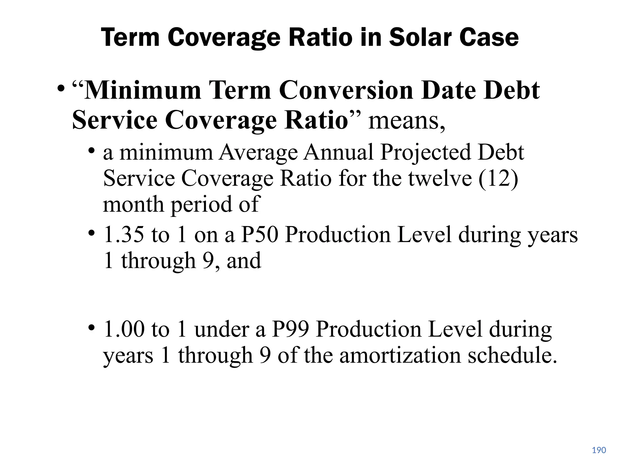
143. Fundamental Formulas for Credit in Project Finance for DSCR,
LLCR and PLCR
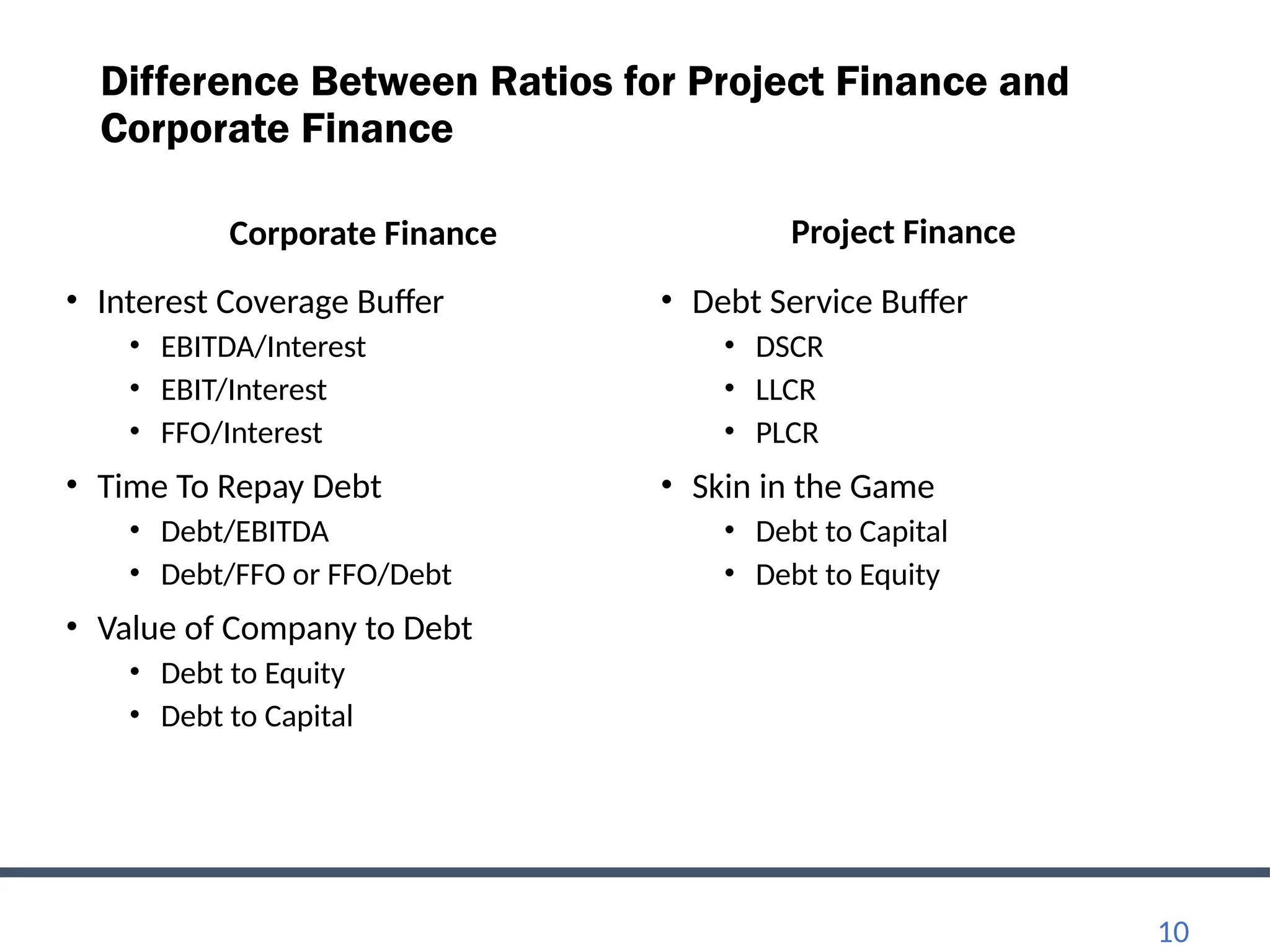
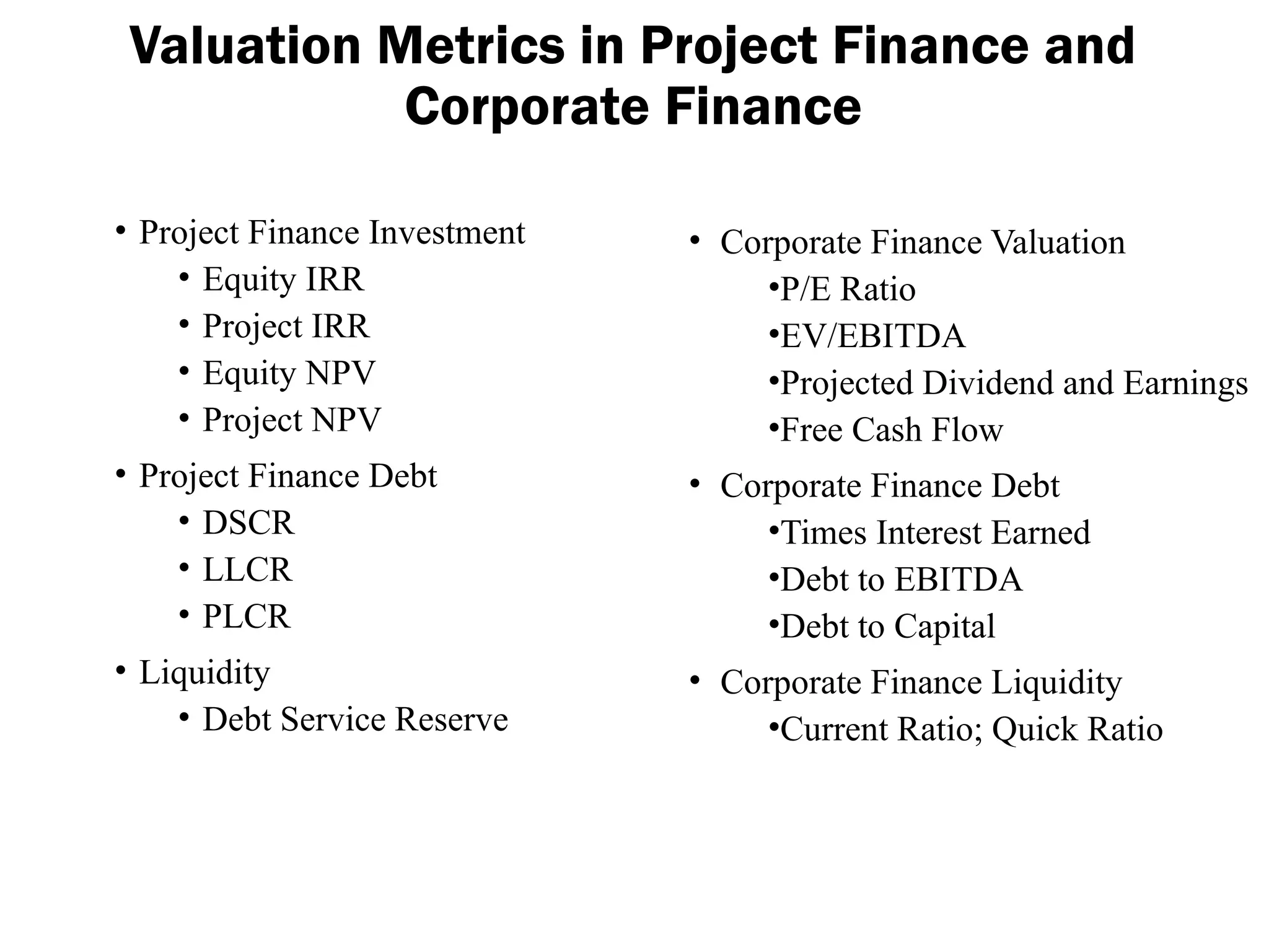
• DSCR = Cash Flow Available for Debt Service/[Debt Service]
• PLCR = PV(Cash Flow Available for Debt Service)/PV(Debt Service)
• LLCR = PV(Cash Flow Available for Debt Service over loan life)/PV(Debt
Service)
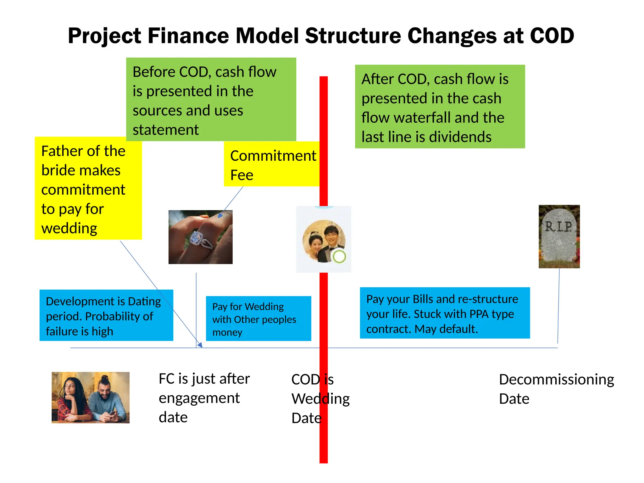
• Debt at COD = PV(Debt Service using Debt Interest Rate)
• Therefore,
• PLCR = PV(Cash Flow Available for Debt Service)/Debt - DSRA
• LLCR = PV(Cash Flow Available for Debt Service over loan life)/Debt – DSRA
• Theory
• Minimum DSCR measures probability of default in one year
• LLCR measures coverage over the entire loan life even if project must be re-
structured
• PLCR measures coverage over the entire project life and the value of the tail

144. • The key behind these ratios is understanding what
they measure. Each ratio can be used to measure how
much cash flow can fall before something bad occurs:
• DSCR: Cash flow reduction before one time default
with formula % reduction = (DSCR-1)/DSCR
• PLCR: Cash flow reduction before loan will not be
repaid by end of project life after restructuring the
loan with the formula % reduction = (PLCR -1)/PLCR
• LLCR: Cash flow reduction before loan will not be
repaid before the end of the loan life even if it must be
restructured. You can measure the cash flow reduction
with % reduction = (LLCR-1)/LLCR.
How to Use the Ratios in Measuring Cash Flow Sensitivity
144

145. • If you have a project with a contract like a
PPA contract or an availability contract, the
cash flows should be stable from year to year.
In this case you would generally focus on the
DSCR.
• In output based projects or commodity based
projects, the cash flow may vary more on a
year to year basis. For these projects you
would more often see the LLCR and PLCR
used.
When Would You Use PLCR and LLCR Rather than Only DSCR
145

146. • The reason that CFADS is discounted at the
interest rate is that if there is a default, it is
assumed that the defaulted amount must be
re-structured and re-paid later on.
• The amount of default is assumed to re-paid
with interest at the same interest of the loan.
• This means that you can compare CFADS
over different time periods
Why Discounting is at the Interest Rate (or the
Debt IRR in the Case of Changing Interest Rate)
146

147. • The tail is the difference between the loan life
and the project life.
• To see what the PLCR measures you can
consider two loans with the same cash flow.
One loan has the same DSCR and PLCR
because the loan has no tail.
• The second loan has a shorter tenor and a tail.
In this case the DSCR will be lower than the
PLCR.
DSCR, PLCR and Value of Tail
147

148. DSCR versus LLCR versus PLCR and Sculpting
DSCR = LLCR = PLCR
DSCR = LLCR < PLCR
Min DSCR < LLCR < PLCR
Level Payment and Tail
Sculpting and Tail
Sculpting and No Tail

149. 149
• Risk allocation matrices will be used to demonstrate how the
DSCR and LLCR can be used to determine acceptable
unmitigated risks:
• The formula:
• break-even cash flow reduction = (DSCR-1)/DSCR.
• Also break-even cash flow over life of loan
• BE reduction = (LLCR-1)/LLCR
• BE reduction for Project Life = (PLCR-1)/PLCR
• Different project finance structures that involve:
• availability payments versus output-based revenues;
• commodity price (merchant) risk;
• traffic or volume risk (pipelines), and
• resource risk (wind, solar and run of river hydro) will be derived.
• For each of the project finance types, an illustrative risk allocation
matrix and project diagram will be developed.
Idea of Risk Allocation Matrix and Use of DSCR, PLCR and
LLCR to Measure Break-Even

150. 150
0.00
20.00
40.00
60.00
80.00
100.00
120.00
140.00
0.00
2.00
4.00
6.00
8.00
10.00
12.00
14.00
16.00
01-janv-79
01-févr-80
01-mars-81
01-avr-82
01-mai-83
01-juin-84
01-juil-85
01-août-86
01-sept-87
01-oct-88
01-nov-89
01-déc-90
01-janv-92
01-févr-93
01-mars-94
01-avr-95
01-mai-96
01-juin-97
01-juil-98
01-août-99
01-sept-00
01-oct-01
01-nov-02
01-déc-03
01-janv-05
01-févr-06
01-mars-07
01-avr-08
01-mai-09
01-juin-10
01-juil-11
01-août-12
01-sept-13
01-oct-14
01-nov-15
01-déc-16
Crude
oil,
average
($/bbl)
Natural
gas,
US
($/mmbtu)
Crude oil, average($/bbl) Volatility29.64%
Naturalgas, US ($/mmbtu) Volatility40.50%
Correlation52.72% Last Valueof Crude oil, average 54.35 Last Valueof
Naturalgas, US 3.26
Natural gas, US ($/mmbtu) Crude oil, average ($/bbl) N/A
Risks of Commodity Prices versus Traffic
Determine the break-even
price relative to historic
prices: Do with DSCR, LLCR
or PLCR

151. • Formulas for Break-Even: Say that you want to know
how big the DSCR should be to cover for an availability
payment that could be reduced by 20%.
• The formulas below are for DSCR; you could also use
LLCR and PLCR
• Break-even cash flow = (DSCR-1)/DSCR
• BE = (DSCR-1)/DSCR
• BE x DSCR = DSCR – 1
• DSCR – BE x DSCR = 1
• DSCR * (1-BE) = 1
• DSCR = 1/(1-BE) or 1/.8 or 1.25
• Note: Be careful with fixed costs. If an oil project has
fixed costs you have to make a more complex formula
You Can Go the Other Way to Find the DSCR
151

152. IRR in Project Finance

153. • Importance of Project IRR. Objective in a sense
is to maximize the equity IRR given a level of
project IRR.
• Danger of high project IRR from banking
perspective. In commodity price analysis means
that others will come into the market and the
margin will be reduced. Must have demonstrated
cost advantage.
• Danger of high project IRR and political risk.
Eventually the government will understand if
the project price is uneconomic
Project IRR or DSCR
153

154. • Project finance uses IRR instead of return on equity
or return on invested capital
• In project finance, the investment on the balance
sheet (net plant) declines investment over the life of
the project.
• If you compute the ROE or the ROIC, the number
starts very small and becomes very large.
• Unless you develop a weighted average that accounts
for the cost of capital and the level of investment on
the balance sheet, it is very difficult to find a good
ROE or ROIC statistic to summarise the project.
IRR versus Return on Investment
154

155. • The equity IRR or Project IRR can be thought of as a
growth rate in cash flow. If there is no intermediate
cash flow, the CAGR and the IRR are the same.
• The problem with the IRR is that cash flow that occurs
before the end of the project (i.e. intermediate cash) is
assumed to be re-invested at the IRR itself. If the IRR
is really high, you may not be able to find another
investment with the same IRR. Further, the MIRR
provides no help to this.
• The IRR can be compared to stock market total
returns.
IRR and Growth Rate in Cash Flow
155

156. • For the IRR, there should be negative cash
flows at the beginning reflecting the investment
followed by positive cash flows.
• In project finance you can compute the project
IRR without tax, the project IRR after tax, the
equity IRR and the debt IRR.
• The project IRR reflects the overall return on
the project and is relatively simple to calculate.
• The after-tax project IRR is the same as the
equity IRR if there would be no debt financing.
Negative Cash Flow and Different IRR’s
156

157. • The debt IRR can be computed from the perspective of debt
holders. The debt drawdowns are the negative cash flow while the
debt service including interest and principal are positive cash
flows. The fees should be included as cash flow. The debt IRR
can be called the effective interest rate or the all-in rate.
• The project IRR is an effective statistic for evaluating the overall
competitiveness of a project. If the project IRR is very high, you
should ask questions about why others cannot create similar
projects and charge a lower price. If the project IRR is below the
cost of debt, you should ask why the project is occurring.
• The equity IRR is the focus of investors because it reflects money
taken out of their pocket relative to dividends received. In
structuring debt terms such as a cash sweep or the debt to capital,
the equity IRR can be used to understand the perspective of the
sponsor.
Project IRR, Debt IRR and Equity IRR Interpretation
157

158. • IRR Statistics from original model
IRR in Solar Case
158

159. Part 3: Availability and Capacity
Based Projects

160. • Economic Theory and Risk Allocation
• Allocation of Risks
• Tricky Allocation of Risks
• Spot Pricing Cons and Pros
Private Public Partnerships and Capacity Based Projects
160

161. Special
Purpose
Vehicle
Off-taker
PPA Contract
Four Part Tariff
Fixed Capacity Charge at Fin
Close
LD Penalty for Delay Risk
Contract O&M Charge
Contract Heat Rate
Availability Penalty
EPC
Contractor
Fixed Price
Contract with LD
O&M
Contractor
Contract with
Guaranteed Heat Rate
and Availability
Penalty
and Fixed Fee
Fuel Supply
Fuel Index
Lenders
Sponsors
Fuel Supply Contract
with Index
Corresponding to
PPA
Loan
Agreement
Shareholder
Agreement
Letter of
Credit for
Equity Cash
EPC
Contractor
Fuel Supply
Fuel Index

162. Basic Equations for Revenue Build Up
• Electricity plants have capacity which is the ability to produce at an
instant
• kW, mW, W
• For producing revenue, there must be some kind of time dimension
attached to the capacity
• Hours, months, years
• kW x h, kW x month, kW x year
• kWh, kW-month, kW-year
• There is a basic distinction in project finance for availability and output
based projects. Output base projects earn revenues on production,
availability based projects earn revenue as long as the plant is available
to produce even if it does not produce.
• Output based projects (renewable): revenue = price x kWh
• Availability based projects (dispatchable): revenue = price x kW-
month

163. Drivers and Cost of Electricity – Slide 1
• Plant Cost and Construction Delay (€/kW or € million/MW or €/W)
• Carrying Charge Rate (% of total cost recovered in a year)
• Annual Capital Cost Recovery: Plant Cost x Carrying Charge or
• Annual Charge per year
• €/kW-year = €/kW x Carrying Charge Rate
• Capacity Factor (% of Time (hours per year plant is running)
• Annual Charge per hour
• Generation = kW x hours operated
• Generation = KW x 8766 hours per year x capacity factor
• Annual Charge per Hour = Annual Charge per year/hours
operated
• €/MW-year = €/kW x Carrying Charge Rate x
1000/Generation

164. Drivers and Cost of Electricity – Slide 2
• Efficiency (Heat Rate)
• Kj/kWh, BTU/MWH, kBTU/MWH, MMBTU/MWH, kWh/kWh
• Fuel Use or Resource Use = HR x Generation
• MMBTU = HR x Generation
• MMBTU = (MMBTU/kWh) x MWh
• Fuel Price
• Measured in €/MMBTU, €/kJ, €/kWh
• Fuel Cost = Fuel Price x Fuel Price
• Fuel Cost/MWH = Fuel Cost/Generation
• Fuel Cost/MWH = HR x Generation x Fuel Price/Generation = HR x Fuel
Cost
• Fuel Cost/MWH = HR x Fuel Price = kJ/MWH x €/kJ (kJ cancels)
• Variable O&M Expense
• Cost that depends on running the plant - €/MWH
• Fixed O&M Expense
• Cost independent of running the plant €/kW -year

165. Risk Allocation and Drivers in PPA
Agreement
Risk in Electricity Production
1. Plant Cost and
Construction Delay
2. Efficiency (Heat Rate)
3. Fuel Price
4. Capacity Factor and
Availability Factor from
Forced and Unforced
5. Variable O&M Expense
6. Fixed O&M Expense
7. Carrying Charge Rate
Allocation of Risk Off-taker and IPP
1. IPP Controls and Takes Risk
2. IPP Control and Risk
3. Off-taker Risk
4. Off-taker Controls Dispatch,
IPP controls Availability
5. IPP Control and Takes Risk
6. IPP Control and Risk
7. Off-taker

166. Begin with Fundamental Question of Risk
Allocation Between Off-taker and PPA
Risk to IPP
• Construction Over-run
• Construction Delay
• Availability
• Efficiency
• O&M Cost Over-runs
• Capacity Amount
Price Mechanism
• Fixed Capacity Charge
• LD in for Delay
• Availability Penalty
• Heat Rate Target
• O&M Fixed Price
• Capacity Payment
Contract Protection
• EPC Fixed Price
• LD in EPC Contract
• O&M Contract LD
• Efficiency
• O&M Cost Over-runs
• EPC and O&M

167. General Purchased Power Agreement Pricing
• Components
• A – Capacity Payment
• Covers debt service, taxes and equity return from project budget
• Deductions for unavailability of plant
• Currency adjustments and currency split
• B – Fixed O&M Charge
• Escalates with general inflation
• Could have currency adjustment
• C – Fuel Energy Charge
• Use the target heat rate
• HR x Fuel Price = Energy Charge
• D – Variable O&M Charge
• Definition of fixed and variable costs
• Start-up costs

168. Four Part Tariff in Availability-based Dispatchable Plants
• If the revenues and profits depend on the availability and not
output but some costs depend on the output of the project then
the pricing structure must be designed to compensate to cover
variable as well as fixed costs. Some costs of producing
electricity are fixed and some are variable, including fuel costs.
Therefore, a variable price must be implemented to cover
variable costs and a fixed charge must be included to cover
fixed charges:
1. Availability Charge: €/kW-month x Available MW
2. Fuel Charge: €/MWh x Energy Production in MWH
• (MWh = MW x hours of production or MW x capacity factor x hours
in period)
3. Variable O&M Charge: €/MWh x Energy Production in MWH
4. Fixed O&M Charge: €/kW-month x Available MW

169. Four Part Tariff Example

170. Tricky Allocation Issues
• Who should take
• Temperature risk when the plant (thermal or
solar) operates less efficiently at higher
temperatures
• Fuel transport risk such as insufficient gas
supply
• Transmission risk if the power cannot be
delivered to the distribution system. Consider
both renewable and thermal.
• Distribution risk if the distribution system cannot
accept the load

171. Drivers and Contracts - Dispatchable
IPP Risks
• Cost of Project, Time
Delay and Technology
Parameters
• Availability Penalty
• Heat Rate Risk
(Adjusted)
• O&M Risk
• Interest Rate
Fluctuation
Contract Mitigation
• EPC Contract with
Fixed Price and LD
(LSTK)
• O&M Contract
• O&M Contract with LD
Provision
• O&M Contract
• Interest Rate Contract
(Fix Rates)

172. Drivers and Profit and Loss Statement -
Dispatchable
• Cost Driver
• Cost x Carrying Charge + Fuel Cost +
Variable O&M + Fixed O&M
• Fuel Cost – HR x Gen x Fuel Pr
• Variable and Fixed O&M
• Capacity Charge Revenue (€/kW-year x
kW)
• Portion of Capacity Charge
• Portion of Capacity Charge
• Portion of Capacity Charge
• Portion of Capacity Charge
• Profit and Loss Account
• Total Revenue from Four Part Tariff
• Fuel Expense
• Fixed and Variable O&M Expense
• EBITDA (Operating Margin)
• Depreciation
• Taxes
• Interest
• Net Income

173. Exercise on Allocation of Risks Outside of IPP Control
• Single price with production risk versus fixed
capacity charge with no production risk
• Effect on DSCR
• Effect on Credit Spread
• Effect on Debt Tenure
• Effect on Equity IRR

174. Problem of Allocating Uncontrollable Risks
• The general idea that risks which can be accepted at a reasonable
cost should be allocated to IPP versus the off-taker. The allocation
process is demonstrated with databases that show the volatility of
commodities and interest rates. For example, fuel price is allocated
to the off-taker because of variation on natural gas, coal and oil
prices.
• But variation in iron prices that cause construction costs to change
are allocated to the IPP. The class discussion involves nuances of
whether risks should be allocated.
• Non-dispatchable plants have a one part tariff while dispatchable
plants have a multi-part tariff. Discussion of resources that discuss
risk allocation are shown below. The left hand figure demonstrates
where to find the resource and the right hand figure shows an
example of the analysis. The first figure illustrates summary slides
and the second slide demonstrates a database of commodity prices.

175. 175
Alternative Way to Look at PF Structure – Key is are Paying
too Much for Risk

176. Significant Emerging Country Defaults (S&P 2007)

177. Other Problem Loans (S&P 2007)

178. Allocation of Risks that Are Out of IPP Control
• Start with capacity factor risk
• What would the IPP want to take the output risk
• If there is surplus capacity, consumers still pay
fixed cost of the plant
• What do you conclude about taking capacity
factor or output risk
• Fuel price risk
• Are the issues with fuel price risk the same as
output risk
• What about negotiating fuel prices

179. Contract Risks

180. Case Study of Risk and Return and Danger of Un-economic
Projects

181. Dabhol Case Study
181

182. Making Money in Different Places by Receiving Money from
PPA Contracts
Special
Purpose
Corporation
(IRR)
Off-taker
pays money
for PPA
PPA – Four Part Tariff
LD for Delay Risk
Fixed Capacity Charge at FC
Contract O&M Charge
Contract Heat Rate
Capacity Charge with Index
Availability Penalty
EPC Contractor:
ENRON
EPC Profit
ENRON O&M
Profit
ENRON –
Fuel Mgmt.
Fee
Lenders
ENRON IRR
on SPV
Fuel
Supply
Contract
Loan
Agreement
Shareholde
r Agreement
Contract
with
Guaranteed
Heat Rate
and
Availability
Penalty
and Fixed
Fee
Fixed
Price
Contract
with LD

183. Dabhol
SPV
Off-taker –
Maharashtra State
Electricity Company
EPC
Management
by Enron
GE Equipment
ENRON –
Fuel Mgmt.
Lenders
Sponsors – Enron,
GE and Bechtel
IRR on SPV
State of
Maharashtra
Federal
Government
of India
OPIC
O&M Contractor
- Enron
Bechtel
Construction
LNG from
Qatar
Off-taker Needs Rate Increase
of 27%-39% to Pay PPA
EPC
Contract
PPA
Contract
Loan
Agreement
Shareholders
Agreement
O&M
Contract
Fuel
Supply
Guarantee
Letter
PRI/PRG
PRI/PRG
Very High Cost of USD
1,400 per kW

184. Dabhol Award for Structuring
184

185. • Economics of the plant
• Careful Benchmarking of Costs
• Ability of off-taker to pay
• Trust in contracts that are not economic
• Compute Project IRR
Issues in Dabhol Case

186. • Read the PDF file with PDF to Excel
• Input the Capital Expenditures and the
Capacity
• Compute the Revenues from the PPA contract
• Assume EBITDA = Capacity Revenues +
Fuel Management Fee Revenues
• Compute Pre-tax IRR Assuming 1 year
construction
Simple Model for Case Study of Availability Project

187. Output Risk in Renewable Energy
187

188. • Wind versus Solar
• Development
• Resource Risk
• Operation and Maintenance
• Transmission Risk
Renewable Energy Introduction
188

189. • “P50 Production Level” means the aggregate
annual energy production level of the Project that
has a probability of exceedance of 50% over a one-
year period of time, according to the Independent
Engineer’s solar production forecasts included in
the report delivered to Administrative Agent.
• “P99 Production Level” means the aggregate
annual energy production level of the Project that
has a probability of exceedance of 99% over a one-
year period of time, according to the Independent
Engineer’s solar production forecasts included in
the report delivered to Administrative Agentt.
P50 and P90 in Solar Case
189

190. • “Minimum Term Conversion Date Debt
Service Coverage Ratio” means,
• a minimum Average Annual Projected Debt
Service Coverage Ratio for the twelve (12)
month period of
• 1.35 to 1 on a P50 Production Level during years
1 through 9, and
• 1.00 to 1 under a P99 Production Level during
years 1 through 9 of the amortization schedule.
Term Coverage Ratio in Solar Case
190

191. Renewable Energy Ratings – Solar PV
191

192. Risk Allocation and Drivers in PPA
Agreement
1. Plant Cost and
Construction Delay
2. Efficiency (Heat Rate)
3. Fuel Price
4. Capacity Factor and
Availability Factor from
Forced and Unforced
5. Variable O&M Expense
6. Fixed O&M Expense
7. Carrying Charge Rate
1. IPP Controls and
Takes Risk
2. IPP Control and Risk
3. Off-taker Risk
4. Off-taker Controls
Dispatch, IPP
controls Availability
5. IPP Control and
Takes Risk
6. IPP Control and Risk
7. Off-taker

193. Drivers and Contracts - Renewable
• IPP Risks
• Cost of Project, Time
Delay and Technology
Parameters
• Capacity Factor Risk
• O&M Risk
• Interest Rate
Fluctuation
• Risk Mitigation
• EPC Contract with
Fixed Price and LD
(LSTK)
• NONE !!!
• O&M Contract
• Interest Rate Contract
(Fix Rates)

194. • Actual case where P50 and P90 were
estimated.
P90 and P50 DSCR with Actual Case

195. • Convert loss diagram into
capacity factor and compare
different cases.
• Difficult to compute
performance ratio from
these diagrams.
• Generally, the loss due to
temperature is the largest
loss factor.
Loss Diagram
Illustration

196. • Everything from standard deviation
• What goes into standard deviation
Understanding Computation of P90 and P99
196

197. • If produced at full capacity factor (kWp) during the day and
nothing at night, the capacity factor would be 50% and the yield
would be 8760/2 = 4380. Just need solar patterns over the day.
Don’t need anything else.
Illustration of STC

198. • Evaluate the P50 and P99 using the DSCR
criteria.
P50 and P99 in Solar Case
198

199. • Compare with Mexico case
Benchmarking Capital Cost – Solar Case
199

200. • Compare O&M Cost
O&M Cost Benchmarking
200

201. Part 4: Effect of Loan Structuring
Provisions on Bidding for Projects

202. 202
Structuring versus Risk Analysis and Bidding for PPA or PPP
Projects
• Importance of project finance loan elements
for different technologies.
• Elements of a term sheet in the context of
both the equity IRR and the bid price.
• Evaluate elements of loan contract for
bidding
• PPP and PPA may be more about structuring
than risk analysis.

203. 203
Effects of Debt Structure on the Bid Price
• The effects of:
• Debt sizing,
• Debt funding
• Debt tenor,
• Debt repayment type, and
• Debt pricing (interest rates and fees)
• Debt Protections
Context of alternative technologies.
Items of a term sheet such as the minimum DSCR, maximum
debt to capital, step-up credit spreads, debt sculpting, debt
funding, DSRA’s, MRA’s and cash sweeps used to evaluate
financial impacts of various financing and timing issues on the
required bid price for a project.

204. • Capital intensity is not just the amount of
capital spent on a project
• It is the capital relative to operating costs
• It includes the lifetime of the project
• Formula:
• Capital Intensity = Capital/Revenues
Definition of Capital Intensity
204

205. 205
Illustration of Effects of Debt Structuring on Capital Intensive
and Non-Capital Intensive Projects

206. 206
Alternative Debt Provisions, Bidding and Carrying Charge
Rate

207. 207
Effects of Financing on Bid Price – Capital Intensive
(5.78)
(15.77)
(8.55)
(2.18)
(8.75) (0.57)
(1.43)
(1.05)
74.64
30.56
0
10
20
30
40
50
60
70
80
90
High
Financing
Cost
74.64
Longer Tenor
- 5 versus 15
68.86
Higher Debt
Percent -
85,00% versus
50,00%
53.09
Lower
Interest Rate -
3,50% versus
7,00%
44.54
Sculpting and
Inflation
42.36
Reduced IRR -
7,50% versus
17,00%
33.61
No Taxes -
0,00% versus
25,00%
33.04
Ballon - 25
versus 20
31.61
Low IRR -
5,50% versus
7,50%
30.56
Best
Financing
Case
30.56
Waterfall Chart for Low Cost Solar with Tracker

208. 208
Effects of Debt Provisions on Fuel Intensive Diesel Technology
(2.71)
(14.46)
(7.84)
(2.21)
(8.41) (0.39) (0.85) (1.04)
157.91
120.00
0
20
40
60
80
100
120
140
160
180
High
Financing
Cost
157.91
Longer
Tenor - 5
versus 15
155.20
Higher Debt
Percent -
85,00%
versus
50,00%
140.74
Lower
Interest Rate
- 3,50%
versus
7,00%
132.90
Sculpting
and Inflation
130.69
Reduced IRR
- 7,50%
versus
17,00%
122.28
No Taxes -
0,00%
versus
25,00%
121.89
Ballon - 25
versus 20
121.04
Low IRR -
5,50%
versus
7,50%
120.00
Best
Financing
Case
120.00
Waterfall Chart for Diesel

209. With Good Financing Structure can Achieve Low Costs

210. Part 5: Nuances of Debt to Capital Constraint
and DSCR Constraint in Different
Circumstances

211. Debt Sizing - Introduction
• Detailed analysis of the term sheet and loan
agreements begins with debt sizing.
• Difference in sizing debt on the basis of:
• maximum debt-to-capital ratio: from cost and
sources and uses
• minimum DSCR: from financial model
• Notion of negotiated base case and downside
for evaluating DSCR.
• Limit the debt to assure equity is in project
and the value of the project is above the debt

212. • Solar Case Debt Size
• Term Loans. The aggregate principal amount of all Term Loans made by
the Lenders outstanding at any time shall not exceed Ten Million Five
Hundred Thousand Dollars ($10,500,000) (the “Total Term Loan
Commitment”).
• $6,471,614, the “Minimum Equity Contribution” or the funding of any
remaining unfunded portion, including by delivery of a letter of credit,
and verification by the Independent Engineer.
• What is the debt to capital ratio
• .
Debt Size in Solar Case
212

213. • Compute the Debt to Capital
Airport Capital Expenditures Compared to Debt
213

214. Debt Sizing – Key Philosophical Question
• Debt to Capital Ratio – Trust sponsor to be smart
enough to not invest in a bad project. Make sure
the sponsor is taking downside risk. With no cash
invested in the project, there is only upside
potential and the sponsor will not care about
downside evaluation. The test is historic
investment and do not have to look forward.
• The notion of DSCR implies that you are smart
enough to make a forecast. If you really believe
your forecast and even variation around your
forecast, you can back into the debt from the
DSCR. This is the notion of negotiated base case
and downside for evaluating DSCR.
• Limit the debt to assure equity is in project and the
value of the project is above the debt

215. 215
Illustration of DSCR and Debt to Capital Constraint
-
20,000.00
40,000.00
60,000.00
80,000.00
100,000.00
120,000.00
140,000.00
160,000.00
180,000.00
200,000.00
01-janv-20
01-août-20
01-mars-21
01-oct-21
01-mai-22
01-déc-22
01-juil-23
01-févr-24
01-sept-24
01-avr-25
01-no
v-25
01-juin-26
01-janv-27
01-août-27
01-mars-28
01-oct-28
01-mai-29
01-déc-29
01-juil-30
01-févr-31
01-sept-31
01-avr-32
01-nov-32
01-juin-33
01-janv-34
01-août-34
01-mars-35
01-oct-35
01-mai-36
01-déc-36
01-juil-37
01-févr-38
01-sept-38
01-avr-39
01-nov-39
01-juin-40
01-janv-41
01-août-41
01-mars-42
01-oct-42
01-mai-43
01-déc-43
01-juil-44
01-févr-45
01-sept-45
01-avr-46
Target DSCR 1.2 Debt/Cap 76% Equity IRR 11.76%
Base Traffic 15,000
Cash Sweep
Debt Service
CFADS
NPV of Debt Service 2,536,916 Debt to Capital Result 76.00%
-
20,000.00
40,000.00
60,000.00
80,000.00
100,000.00
120,000.00
140,000.00
160,000.00
180,000.00
200,000.00
01-janv-20
01-août-20
01-mars-21
01-oct-21
01-mai-22
01-déc-22
01-juil-23
01-févr-24
01-sept-24
01-avr-25
01-no
v-25
01-juin-26
01-janv-27
01-août-27
01-mars-28
01-oct-28
01-mai-29
01-déc-29
01-juil-30
01-févr-31
01-sept-31
01-avr-32
01-nov-32
01-juin-33
01-janv-34
01-août-34
01-mars-35
01-oct-35
01-mai-36
01-déc-36
01-juil-37
01-févr-38
01-sept-38
01-avr-39
01-nov-39
01-juin-40
01-janv-41
01-août-41
01-mars-42
01-oct-42
01-mai-43
01-déc-43
01-juil-44
01-févr-45
01-sept-45
01-avr-46
Target DSCR 1.2 Debt/Cap 95% Equity IRR 15.58%
Base Traffic 15,000
Cash Sweep
Debt Service
CFADS
NPV of Debt Service 3,028,608 Debt to Capital Result 89.80%
Lower DSCR results in
too high debt to
capital ratio. Need to
constrain the debt.
Discounted Red Area
(using the interest rate)
is the Value of the
Debt.
DSCR sizing means you
believe your forecast.

216. 216
Which Constraint is in Place
• Items have an effect on whether the debt to capital constraint
or the debt to capital constraint applies:
• Need to Understand that NPV of Debt Service is Loan Value
• High Project IRR  More Likely Debt to Constraint;
• Long Tenor  More Likely Debt to Capital Constraint;
• Sculpting  More Likely Debt to Capital Constraint;
• Low Interest Rate  Morel Likely Debt to Capital Constraint.
• Low Project IRR  More Likely DSCR Constraint;
• Short Tenor  More Likely DSCR Constraint;
• Level Payment  More Likely DSCR Constraint;
• High Interest Rate  More Likely DSCR Constraint

217. 217
Evaluation with Geometry and NPV Formula

218. • Input Minimum DSCR
• Compute Target Debt Service
• Compute PV of Debt Service
• Use PV of Debt Service as Debt in Sources
and Uses
• Compute PV of CFADS
• LLCR for Max Debt to Cap is PV of CFADS
divided by Cost * Debt/Cap
Model with Debt Sculpting
218

219. 219
Sculpting Equations - Basic
• One of the main ideas about the repayment process in project finance is
that the modelling is much more effective when you combine formulas
with other excel techniques. If you try and solve these things with a brute
force method that uses a copy and paste method or goal seek things will
get very messy. Formulas used for repayment and debt sizing are listed
below: The fundamental two sculpting formulas are:
• (1) Target Debt Service Per Period = CFADS/DSCR
• (2) Debt Amount at COD = PV(Interest Rate, Target Debt Service)
• Non-Constant Interest Rates
• However this is by no means the only formula you should use when
working on repayment. In cases when the interest rate changes, a simple
present value formula cannot be used. Instead, an interest rate index can
be created that accounts for prior interest rate changes as follows:
• (3) Int Rate Index(t) = Int Rate Indext-1 x (1+Interest Rate(t))
• (4) Debt Amount at COD = ∑ Debt Service(t)/Interest Rate Index(t)

220. 220
Sculpting Equations with Debt to Capital Constraint
• Use of LLCR when there is a Target Debt to Capital constraint
that drives the amount of the debt. If the debt is being sized by
the debt to capital ratio, a higher DSCR must be used.
• This raises the issue of how to compute sculpted debt
repayments when debt is sized with the debt to capital ratio
and the DSCR is not from the DSCR constraint.
• When the Debt is Sized by Debt to Capital the LLCR can be
used to size the debt, because with sculpting, the DSCR =
LLCR. Formulas in this case include:
• (5) Target Debt Service(t) = CF(t)/LLCR
• (6) LLCR = NPV(Interest Rate, CFADS)/Max Debt from Debt to
Capital
• (7) DSCR Applied = MAX(Target DSCR,LLCR with Max Debt)

221. 221
Sculpting Equations with LC Fees
• Adjusting Sculpting Equations for Debt Fees: Debt fees such as the fee on a letter
of credit is part of debt service. To include the fees in the sculpting equations, you
should subtract the fees when you compute the net present value of debt, as the
fees reduce the amount of debt service that can be supported by cash flow. To make
the sculpting work you should also make the repayment lower by the fees as shown
below:
• (14) Repayment = CFADS/DSCR - Interest - Fees
• (15) Debt = NPV(Interest Rate, Debt Service-fees)
• Debt = NPV(rate, Debt Service) - NPV(rate, Fees)
• Note Debt Service in the above equation means debt service without fees and debt
is reduced by PV of fees
• Adjusting LLCR for Debt Fees: The sculpting analyses include calculation of the
LLCR to evaluate whether the debt to capital constraint is driving the constraint. In
this case the PV of CFADS is not the correct numerator for the analysis. Instead,
the PV of the LC fees should be added to the denominator of the LLCR as follows:
• (16) LLCR = PV(CFADS)/(Debt + PV of LC Fees), where
• (17) Debt = Project Cost x Debt to Capital

222. • Sculpting and Changes in the DSRA balance including Final
Repayment
• After working through letters of credit for the DSRA, taxes, interest
income and other factors that cause difficult circular references, the
final subject addressed is using the DSRA to repay debt.
• A similar result occurs when changes in the DSRA are included in
CFADS. Incorporating these changes in a financial model without
massive circularity disruptions can be tricky, but it can be solved by
separately computing the present value of changes in the DSRA.
• Changes in the DSRA can be modelled using the following equations:
• (18) Debt Adjustment = PV(Interest Rate, Change in DSRA/DSCR)
• (19) Repayment = Repayment from Normal Sculpting + Change in
DSRA/DSCR
Sculpting with DSRA as Final Payment
222

223. Part 6: Debt Sizing: Including Items in Project Cost
(such as development fees and owners cost) that
do not Involve Cash Outflow to Increase Returns

224. Reconciling Debt to Capital with DSCR
224
Try to increase tenor
to reduce increase
the DSCR
Cash Flow results in
too high DSCR
meaning that you
have debt to cap
constraint
No
Yes
Increase the project
cost WITHOUT
spending money on
things like land value
After you are finished with the
term sheet it looks like the DSCR
constraint and the debt to
capital constraint give you the
same answer. This could be
because of the process.

225. 225
Effects of Non-Cash Increases in Project Cost
• When does asset increase matter and when does it not
• Importance of paying cash or not paying cash
• Examples of non-cash increases in project cost
• Development fees
• Owner costs
• Some development costs
• Contingencies
• Value of Land allocated to project
• EPC profit if EPC is sponsor
• Games with EPC profit
• Items that can increase the cost of a project affect returns
primarily when the debt to capital constraint applies and have
less or no importance when the DSCR drives debt capacity.

226. 226
Debt Sizing: Including Items in Project Cost that do not
Involve Cash Outflow
• Accounting allocations to the project can have large effects on the
equity IRR through debt sizing derived from the debt to capital
ratio.
• If the DSCR drives debt sizing, the accounting allocations, fee
allocations and other adjustments have no effect on the equity
IRR.
• Accounting allocations and non-cash contributions can change the
structure of returns when multiple investors are involved in the
project. If one party is allowed to include non-cash allocations as
the basis for his investment, his return is much higher.
• Depending on the manner in which project costs are accounted for,
multiple investors pay debt service and receive dividends, but the
investor who did not invest as much cash effectively borrows less
relative to the cash investment.

227. 227
Debt Sizing: Profits from EPC Contractors or O&M Contractor
when Investor is also Contractor
• If the EPC profits do not affect the debt size and there is
only one investor, placing profits at the EPC contractor level
or the investor level does not influence overall returns (i.e.
if DSCR drives debt size).
• Depending on whether the debt to capital constraint applies
or there are multiple investors, EPC profits can increase
equity IRR (by increasing the debt size).
• Cash Flow Waterfall and issues associated with including
profits in O&M contract rather than in SPV cash flow.
Profits on the O&M contract versus including O&M costs at
the SPV level can affect the distribution of dividends as the
O&M fee is paid before debt service.

228. Special
Purpose
Vehicle: Bond
Rating of A-
Off-taker: Korea and Japan
Utility Companies: Want
strong off-taker with
inactive to honor contract
O&M
Contractor
Lenders:
Issued bonds and
debt with long tenor
and low rates
Sponsors:
Want strong
sponsor:
Mobil
State Loan
Agreement
O&M
Agreement
Off-take Contract
with minimum
supply but no fixed
price
O&M Contractor is Sponsor
Profits to O&M
Reduce the SPV
Cash Flow. O&M
paid before debt
service

229. 229
Illustration of Non-Cash Accounting

230. 230
Development Fee Theory
• Development fees can be a percent of project cost or a multiple of
the amount spent on development.
• This yields big profits to developers when the notice to proceed
occurs and can be a cash outflow for the sponsor. The big profit
accounts for the low probability of success during development.
• If the developer and the sponsor are the same, this profit is not a
cash outflow from the perspective of the project.
• Better to put development fees into cost with debt to capital
constraint

231. Enron Power
Philippines Corp
Philippines
Government
Enron
Corp.
113MW
Subic
Power
Corp.
Philippine
Investors
15-year
BOT
Concession
Napocor
Supply
Fuel Free
•Capacity Charge
•O&M Charge
•Energy Charge
PPA
Enron Power
Operating Co.
Turnkey
Construction
Contract
Completion
Guarantee
Equip’t Cos. Warranties
US$105 million, 15-year Notes
Buyout
Rights
Enron Subic
Power Corp
O&M
Agreement
Performance
Undertaking
Ground
Lease
Insurances
Fluor Daniel
Enron Power
Phils. Op’g Co.
EPC
65%
35%
Case Study - Funding
Enron - Subic Bay, Philippines

232. Sources of Funds:
Notes $ 105 M
Subordinated Note 7
Equity of Sponsor 28
Working Capital 2
TOTAL $ 142
Uses of Funds:
Turnkey Contractor $ 112 M
Bonus to Turnkey Contractor 7
Development and other related costs and Fees 14
Pre operating, Start-up and Commissioning Costs 3
IDC 4
Working Capital Loan 2
TOTAL $ 142
113 MW Diesel Generator Power Station
Subic Bay, Philippines

233. • Equity Contribution.
• (i) evidence (including copies of invoices and
other documentation, as reviewed and
confirmed by the Independent Engineer) of
the payment of Project Costs in connection
with the development and construction of the
Project on or prior to the Closing Date
Development Cost Documentation
233

234. BOT/PPA Contract
• 15 year BOT and toll process
• NAPOCOR (government owned generation company) to
supply fuel & take electricity - no fuel availability risk
• Capacity fee $21.6/kW/month on available capacity
• Capacity fee is dollar denominated – no direct foreign
exchange risk, overseas a/c
• O&M fixed fee and energy fee is in Peso - $4.56/kW/Month
• heat rate penalty & bonuses
• buy out rights @ NPV capacity fees- late payment, change
of BOT law, war, etc.

235. • Add Development Fee to Sources and Uses
• Adjust the Equity IRR for Development Fees
Received
• Adjust Model to have Debt to Capital
Constraint
• Use Goal Seek to Compute Development
Fees
Adjustments for Development Fee
235

236. Part 7: Debt Funding: Nuanced Issues with
Pre-Commercial Cash Flow and Equity Bridge
Loans

237. Up-Font Equity in Solar Case
237

238. • In general, debt funding is difficult without some kind of
support from outside of the project.
• If the project return is above the interest rate, equity return
increases when the equity is contributed later and debt
earlier.
• From bank perspective, the equity should be put in first
and the loan in last.
• Specific Issues:
• Funding of equity first or pro-rata
• Capitalisation of interest
• Pre-operating cash flow
• Interest on sub-debt or shareholder loan
• Equity bridge loan
Issues with Funding
238

239. • When a borrower uses cash during
construction, the funding request includes:
• Notice of Borrowing
• Payment and draw details
• Construction certificate
• Schedule of construction costs and cumulative
amounts
• Insurance certificates
• Financial reports and other documents
Draw Request and Funding - Introduction

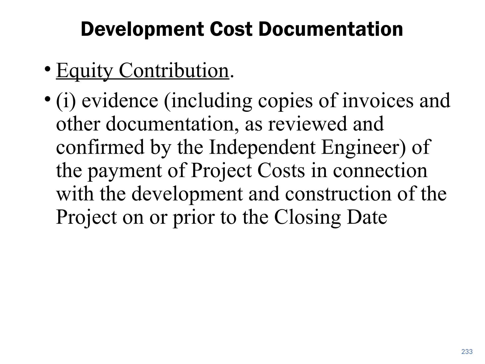
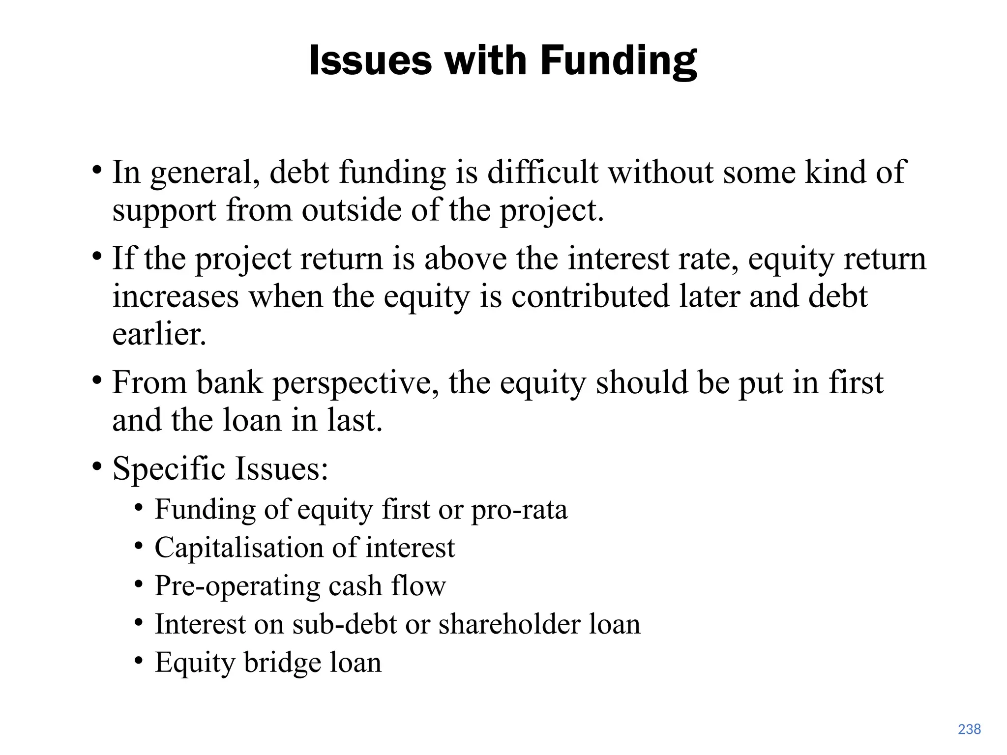
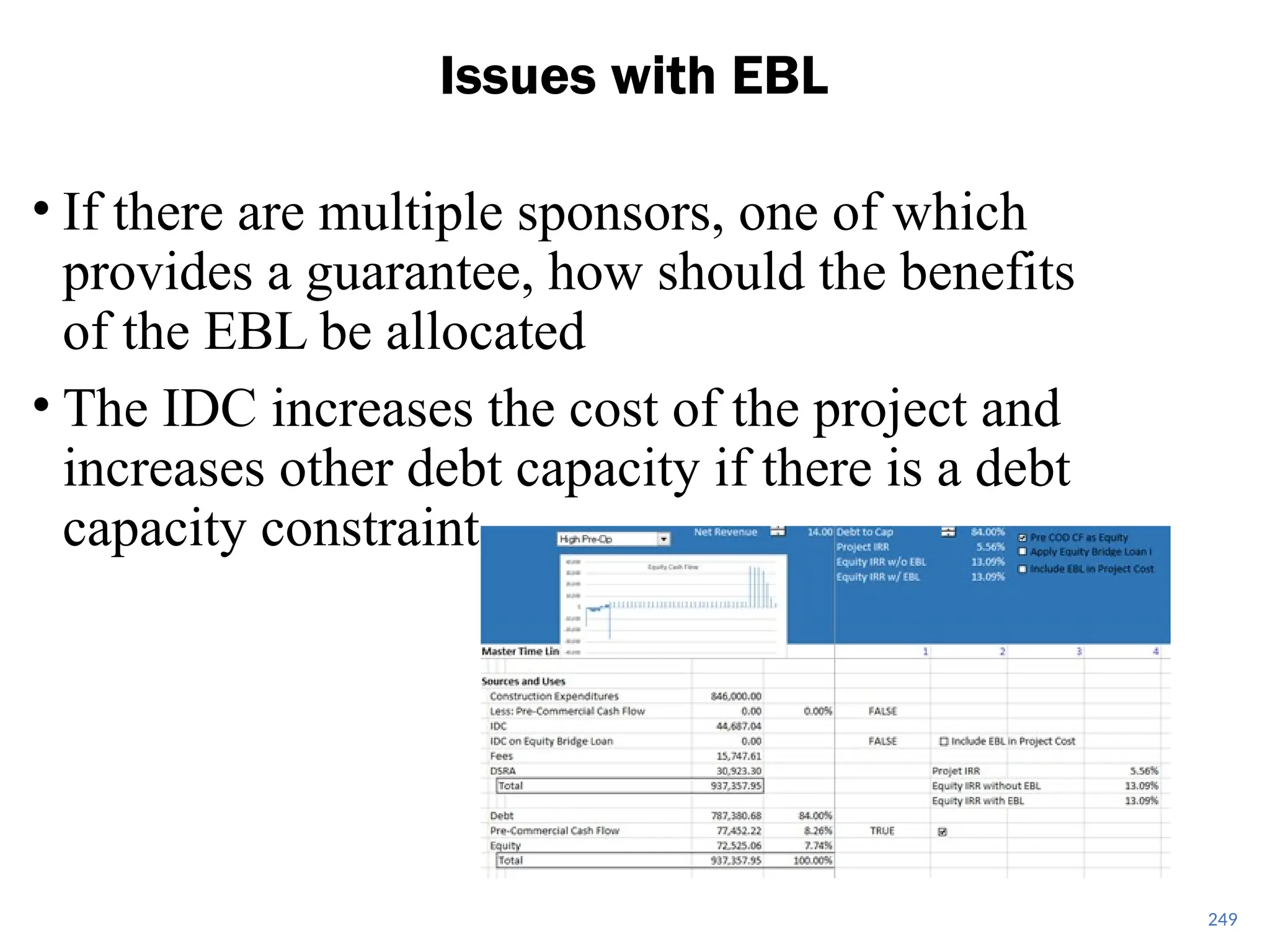
240. • Prior to satisfying the options conditions, it is the
usual practice for the financiers to:
• be able to rely on other contractual or financial resources
(recourse or some kind of support from sponsors) to repay
that funding [if the project fails to be completed];
• If equity is not up-front may require letter of credit,
sponsor guarantee or really strong EPC contract; and,
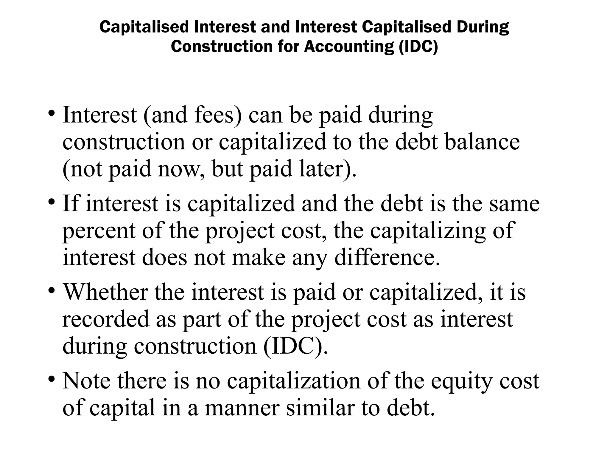
• to roll up the capitalized interest-during-construction
(“IDC”) into the financing (i.e. capitalizing interest).
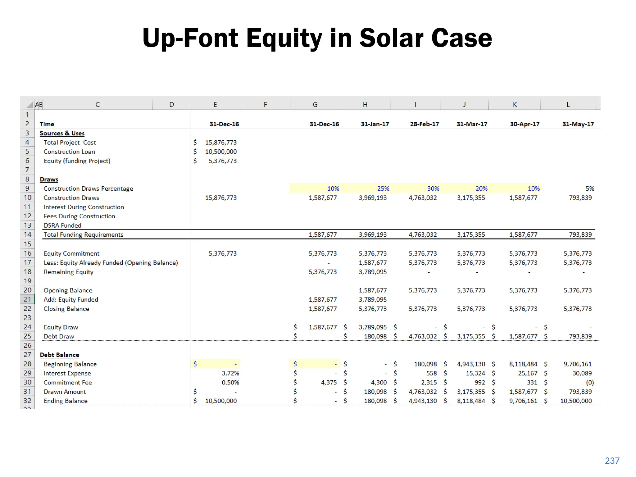
• During the construction phase, equity and debt funds
are used to finance the project construction with
funds generated from the project cash flow covering
the operation period.
Project Finance Loans – Drawdown during Construction
(Reference)

241. • Interest (and fees) can be paid during
construction or capitalized to the debt balance
(not paid now, but paid later).
• If interest is capitalized and the debt is the same
percent of the project cost, the capitalizing of
interest does not make any difference.
• Whether the interest is paid or capitalized, it is
recorded as part of the project cost as interest
during construction (IDC).
• Note there is no capitalization of the equity cost
of capital in a manner similar to debt.
Capitalised Interest and Interest Capitalised During
Construction for Accounting (IDC)

242. Nuanced Issues with Pre-Commercial Cash Flow
• The effects of accounting for pre-commercial cash
flows as either equity or reduction in project cost.
• In terms of accounting, pre-commercial cash flow is
income and should be part of equity.
• Alternatively, one could call the pre-commercial cash
flow a reduction in the cost of the asset.
• Related issues include the issue of government grants
and early production.
• With an extreme case the labelling the pre-commercial
cash flow as equity results in improved returns but
from banker’s perspective is not “skin in the game.”

243. 243
Illustration of Accounting for Pre-commercial Cash Flow
Note the
operating cash
flow is included
as equity. More
than the Paid in
equity.

244. Special
Purpose
Vehicle: Bond
Rating of A-
Off-taker: Korea and Japan
Utility Companies: Want
strong off-taker with
inactive to honor contract
EPC Contractor:
Kellogg with
Strong Record
and Finances
EPC: Fixed Price
Contract with LD
O&M
Contractor
Supplier: Need
to Understand
Economics and
Supply Curve
Lenders:
Issued bonds and
debt with long tenor
and low rates
Sponsors:
Want strong
sponsor:
Mobil
State
Loan
Agreement –
Draws Green;
Debt Service
Red
O&M
Agreement
Supply
Agreement
Off-take Contract
with minimum
supply but no fixed
price
Review Basic Project Finance Diagram
Shareholder
Agreement

245. Multiple Projects with Separate SPV’s

246. Special Purpose Vehicle: - Combine
Projects
Lenders:
Issued bonds and
debt with long tenor
and low rates
Sponsors:
Want strong
sponsor:
Mobil
State
Loan
Agreement –
Draws Green;
Debt Service
Red
Project Finance Diagram – Multiple Projects with Single SPV
Shareholder
Agreement
Project 1 Project 2 Project 3
Project 4
Green is debt
contribution, red
is debt service
and fees
Green is equity
contribution, red
is dividends

247. Equity Bridge Loans and Recourse Debt
• In some projects, equity holders provide loans to the project from
their balance sheet instead of equity.
• Example
• A project finance transaction is structured with equity first
financing (i.e. equity put in to finance construction before debt).
• The sponsor secures a separate loan to finance its equity
requirements, meaning it does not put any equity when you
count the corporate side.
• The loan will be re-paid in a bullet (with interest capitalised) at
the end of the construction period or maybe even later.
• When the loan is re-paid, the sponsor provides equity to finance
the loan.
• The equity bridge loan must have a parent guarantee.

248. Nuanced Issues with Equity Bridge Loans
• In pure project finance, equity should be contributed before debt during
the construction period to assure that equity does not walk away from
the project during construction.
• Pro-rata debt and equity contributions or equity bridge loans require
some kind of sponsor support and can in theory distort the equity cash
flow.
• An equity bridge loan requires parent support, the cost of which is not
included in the equity IRR. The effects of IDC on equity bridge loan on
project taxes and the effects of equity bridge loans in different interest
rate environments and on different types of projects will be discussed.
• Issue
• Should the equity bridge loan be included in computing Equity
IRR.
• The loan uses resources of the parent and must be guaranteed by
the parent

249. 249
Issues with EBL
• If there are multiple sponsors, one of which
provides a guarantee, how should the benefits
of the EBL be allocated
• The IDC increases the cost of the project and
increases other debt capacity if there is a debt
capacity constraint

250. Nuanced Issues with IDC on Shareholder Loans
• Shareholder loans seem to have no effect on
senior debt. All of the covenants and waterfall
issues occur after the senior debt is paid.
• If senior debt limits the dividends to
shareholders, it will also limit the shareholder
loan payments
• Equity IRR should consider the shareholder loan
and any other equity as combined cash flows
• The shareholder loan may affect taxes which will
increase the cash flow (and cause a circular
reference problem).

251. Standby Loans for Construction Cost Over-run and the Issue of
Cost Under-run
• With a cost over-run facility, the commitment
fee can increase the cost of the project.
• If the debt is subordinated to senior debt the
over-run facility is similar to shareholder
loans.
• If there is a cost under-run and the debt has
been committed with and EBL or pro-rata, a
question arises as to whether the debt should
be reduced or whether the proceeds should
accrue to shareholders.

252. Evaluation of Delays in Construction
• In evaluating delays in construction, it is
generally better not to change the S-curve but
rather to assume there is dead time.
• After accounting for the reductions in PPA
revenues, the liquidated damage can accrue to
reduction of debt to maintain the DSCR.

253. 253
Complex IDC Calculations with Portfolios
• The IDC calculations can be complex if some
parts of the project are completed while others
are continuing to be constructed.
• This is a typical problem in real estate and solar
roof-top
• To resolve the problem:
• Keep track of plant in service and construction work
in progress in separate accounts
• Allocate interest from the ratio of CWIP to (CWIP
+ Plant in Service)
• IDC itself will also be in CWIP and Plant in Service

254. Draw-downs and Management of Disbursement of Funds
• The strict control of fund disbursements can provide
a mechanism to maintain leverage over contractors
and thus help to minimize construction risk in the
better rated projects.
• Loan documents typically give lenders the right to
closely monitor construction progress and release
funds only for work that the lender's engineering and
construction expert has approved as being complete.
• Third-party trustees, acting in a fiduciary capacity,
will generally manage disbursement of funds to
protect debtholders' interest in the project. (Multiple
Investors)

255. • Retention of all debt-financed funds in a segregated account
by a trustee experienced in management of power project
construction, preferably an experienced bank or other lender
for these projects;
• Payment structures that retain a small portion of each amount
payable, about 5%, until the project reaches commercial completion;
• Disbursements made only for work certified as complete by an
independent project engineer retained by the construction trustee
solely for approving disbursements;
• Right to suspend or halt disbursements when the trustee concludes
that construction progress is materially at risk (reversals or
revocations of necessary regulatory approvals or changes in law or
cost outside the levels anticipated by the budget and schedule)
• Authority to approve all change orders or authority to limit
change orders to a pre-determined amount (example MCV)
Draw-downs and Retention of Funds

256. 256
Credit Enhancements - Introduction
• Various added provisions that are included in loan
agreements to provide additional protection to lenders.
• These provisions that can include:
• DSRA’s
• MRA’s
• Cash sweeps
• Dividend lock-up covenants
• While the credit enhancements can be the subject of
intense negotiation, they cannot change a failed project
into a good project from a lender perspective.
• Instead, they can only either limit dividends or reduce the
amount of effective net debt associated with a project.

257. Part 9: Debt Repayment Structure: Sculpted Repayment and
Nuanced Issues associated with Debt to Capital or DSCR
Constraints Combined with Repayment Patterns

258. • The structure of debt (the draw down and term to
maturity) can seem to have more important impacts
on the value of a project than the size of the debt and
certainly more than the interest rate on the debt.
• Average life is the general way in project finance to
measure the length of the debt although duration is a
is better way in theory to measure the effective term
of the debt.
• The debt structure should depend on the economic
characteristics of a project such as the revenue and
expense contracts. But it may be able to re-finance
debt.
Debt Repayment - General

259. • Airport Case
• Tranche A Final Maturity Date means 15 June
2020.
• Tranche B Final Maturity Date means 15 June
2023.
• Maturity in Solar Case:
• Mini-Perm 9 Year
• Amortisation 17.25
• Maturity and the economic life of the project
Maturity in Cases
259

260. 260
Multiple Capacity Charges and Optimisation of Debt
Repayment
• For some countries and financial institutions, DSCR
constraints and debt repayment patterns are given.
• In these cases, synthetic sculpting can be developed
with alternative tariff structures that have a step down
element (Malaysia, Pakistan).
• In other cases a flexible maintenance contract can be
used to create synthetic sculpting (Brazil).
• Incentive issues associated with step-down tariffs
where sponsors can have an incentive to walk away
from the project and techniques to measure the cost
and benefits of alternative maintenance structures will
be addressed as part of the session.

261. Example of Repayment (Bullet Not Shown)
• Loan tenor is
explained by the
repayment period is
still within the PPA
terms (i.e. 20 years
from PCOD), giving
a one year tail, and
the project is a Build,
Own and Operate
(BOO) and a BOOT.

262. Sculpting versus Equal Installment with DSCR Constraint
Note the big increase in IRR with the DSCR constraint – because of
the larger debt size. Recall that can effectively make the DSCR
constraint be in place

263. Sculpting versus Equal Installment with Debt to Capital
Constraint

264. 264
Alternative Repayment Patterns
• Given a DSCR constraint and the formula that the
present value of debt service equals the amount of debt
at COD, use geometry to maximize debt.
• The general idea of maintaining a constant DSCR over
the life of a project in sculpting when the risks can
increase over time.
• Contrasts to the requirement that banks must increase
capital with longer terms and that an implicit assumption
of constant credit spreads is increasing risk over time.
• Sculpting versus alternative methods in the context of
different revenue patterns (indexation, flat fee-in tariffs,
tax depreciation, etc.)

265. 265
Complex Sculpting Issues
• Complex sculpting issues can involve:
• Letter of credit fees
• Balloon payments as a percent of the loan
amount
• Interest income on sweeps for balloon payment
• Taxes and net operating losses
• DSRA as final debt payment
• To resolve these issues use equations and
some fancy excel. Do not try to use brute
force.

266. 266
Example of Synthetic Sculpting with O&M Payments

267. • Computation of borrowing base
• Debt repayment and borrowing base – must pay-
off debt that is below the maximum borrowing
base
• Rational for borrowing base
• Rate of production extraction
• Problems with borrowing base
• Declining prices and acceleration of loan re-payments
• Increasing prices and reduction of loan re-payments
• Modelling of borrowing base
Borrowing Base and Resource Transactions

268. DSCR
Debt to
Capital Tenor SIBOR Dev Fee Equity IRR Avg Debt Life Constraint
Weighted
Average
Margin
Base Case 1.25 85.00% 20 Increasing Marrgin2.50% 20 1 5.41% 11.90 Debt from DSCR 2.30%
Aggressive Case 1.20 85.00% 22 Fixed Margin 1.50% 50 2 12.35% 12.78 Debt to Capital constraint 1.75%
Conservative Case 1.30 70.00% 18 Conservative Margin
3.00% 0 3 4.16% 10.94 Debt from DSCR 3.00%
DSCR Aggressive Case 1.20 85.00% 20 Increasing Marrgin2.50% 20 4 5.46% 11.90 Debt from DSCR 2.30%
Debt to Capital Aggressive Case 1.25 85.00% 20 Increasing Marrgin2.50% 20 5 5.41% 11.90 Debt from DSCR 2.30%
Tenor Aggressive Case 1.25 85.00% 22 Increasing Marrgin2.50% 20 6 5.55% 13.19 Debt from DSCR 2.34%
Credit Spread Aggressive Case 1.25 85.00% 20 Fixed Margin 2.50% 20 7 6.29% 11.87 Debt from DSCR 1.75%
Aggressive Case 1.25 85.00% 20 Increasing Marrgin1.50% 20 8 7.56% 11.60 Debt from DSCR 2.30%
SIBOR Aggressive Case 1.25 85.00% 20 Increasing Marrgin2.50% 50 9 5.41% 11.90 Debt from DSCR 2.30%
DSCR Conservative Case 1.30 85.00% 20 Increasing Marrgin2.50% 20 10 5.37% 11.90 Debt from DSCR 2.30%
Debt to Capital Conservative Case 1.25 70.00% 20 Increasing Marrgin2.50% 20 11 5.39% 11.90 Debt to Capital constraint 2.30%
Tenor Conservative Case 1.25 85.00% 18 Increasing Marrgin2.50% 20 12 5.31% 10.64 Debt from DSCR 2.25%
Credit Spread Conservative Case 1.25 85.00% 20 Conservative Margin
2.50% 20 13 4.34% 12.13 Debt from DSCR 3.05%
Conservative Case 1.25 85.00% 20 Increasing Marrgin3.00% 20 14 4.66% 12.05 Debt from DSCR 2.30%
SIBOR Conservative Case 1.25 85.00% 20 Increasing Marrgin2.50% 0 15 5.41% 11.90 Debt from DSCR 2.30%
Equity IRR without Balloon
268
Data table with structuring – need to use
macro instead of basic data table

269. Equity IRR with Balloon
269
DSCR
Debt to
Capital Tenor SIBOR Dev Fee Equity IRR Avg Debt Life Constraint
Weighted
Average
Margin
Base Case 1.25 85.00% 20 Increasing Marrgin2.50% 20 1 5.99% 11.85 Debt from DSCR 2.30%
Aggressive Case 1.20 85.00% 22 Fixed Margin 1.50% 50 2 65.75% 12.78 Debt to Capital constraint 1.75%
Conservative Case 1.30 70.00% 18 Conservative Margin
3.00% 0 3 3.09% 11.14 Debt from DSCR 3.00%
DSCR Aggressive Case 1.20 85.00% 20 Increasing Marrgin2.50% 20 4 6.16% 11.85 Debt from DSCR 2.30%
Debt to Capital Aggressive Case 1.25 85.00% 20 Increasing Marrgin2.50% 20 5 5.99% 11.85 Debt from DSCR 2.30%
Tenor Aggressive Case 1.25 85.00% 22 Increasing Marrgin2.50% 20 6 6.50% 13.12 Debt from DSCR 2.34%
Credit Spread Aggressive Case 1.25 85.00% 20 Fixed Margin 2.50% 20 7 7.99% 11.87 Debt from DSCR 1.75%
Aggressive Case 1.25 85.00% 20 Increasing Marrgin1.50% 20 8 11.54% 11.54 Debt from DSCR 2.30%
SIBOR Aggressive Case 1.25 85.00% 20 Increasing Marrgin2.50% 50 9 5.99% 11.85 Debt from DSCR 2.30%
DSCR Conservative Case 1.30 85.00% 20 Increasing Marrgin2.50% 20 10 5.86% 11.85 Debt from DSCR 2.30%
Debt to Capital Conservative Case 1.25 70.00% 20 Increasing Marrgin2.50% 20 11 5.90% 11.85 Debt to Capital constraint 2.30%
Tenor Conservative Case 1.25 85.00% 18 Increasing Marrgin2.50% 20 12 5.71% 10.60 Debt from DSCR 2.25%
Credit Spread Conservative Case 1.25 85.00% 20 Conservative Margin
2.50% 20 13 4.14% 12.07 Debt from DSCR 3.05%
Conservative Case 1.25 85.00% 20 Increasing Marrgin3.00% 20 14 2.97% 12.29 Debt from DSCR 2.30%
SIBOR Conservative Case 1.25 85.00% 20 Increasing Marrgin2.50% 0 15 5.99% 11.85 Debt from DSCR 2.30%
This case assumes large balloon payment at
the end of the life – 20%. Note how the equity
IRR increases.

270. Part 7: Repayment Tenure: Length of Debt
Repayment, Mini-perms, Bullet Repayments
and Re-financing

271. • Now move to the length of the debt or the debt
tenure
• In corporate finance, debt is re-financed continually
and the debt to capital is developed on a market
value basis.
• In project finance, the initial assumption is that debt
to capital reduces and for a portion of the project
life the total financing can come from equity.
• In reality, if a project is performing well, it will be
sold and/or re-financed. Continual re-financing can
result in a similar outcome a very long-term debt.
Re-financing, Corporate Finance and Project Finance

272. • A project's debt amortization schedule often
influences the rating, more so than the degree of
leverage.
• Front-loaded principal amortization schedules
that capitalize on the more predictable project
cash flows in the near term may be less risky that
those with whose delayed amortizations seek to
take advantage of long-term inflation effects.
• Flexible re-payment structures can be developed
where the project has irregular cash flows.
Debt Repayment Structure and Risk

273. • It seems that the debt tenure is more
important than the interest rate (depending on
the relationship between the project return
and the interest rate).
• You can try some different debt amounts and
interest rates and see how the length of the
debt is an crucial element (two way data
tables).
• The problem with this is that it does not
account for re-financing.
Debt Tenure and Return
273

274. • Commercial Bank Market
• Up to 15 years
• Private Placement Market
• Up to 20 years
• Rule 144A
• Up to 30 Years
• Requires investment grade rating
• Project Finance average maturity 8.6 years
Statistics on Project Finance Debt Tenor

275. Fundamental Effect of Debt Tenure with Debt to Capital
Constraint
275

276. • There is a fundamental philosophical and
strategic issue about re-financing in project
finance.
• The above charts are distorted because of the
assumption that there is no re-financing.
• With re-financing, the effect of the debt tenure
is much less if not reduced to almost nothing.
• Assuming no re-financing is a very negative
assumption (like and oil price of zero because
we cannot predict everything).
Re-financing Changes Everything
276

277. • The table below illustrates the relationship
between the length of the debt and the
interest rate in terms of equity IRR.
• Note that the length makes more difference
than the interest rate (with no re-financing)
Debt Length and the Interest Rate Assuming Size Driven by
Debt/Capital Ratio
277

278. • The table below illustrates the relationship between the length
of the debt and the debt to capital ratio in terms of equity IRR.
• Note that the inter-relationship between the length of the debt
and the leverage.
• But the length of the debt still has a big effect (again without
re-financing).
Debt Length and the Debt to Capital
Ratio
278

279. 279
Mini-perms
• Matching the tenor of repayment to the life of the project and
even considering terminal value in the repayment in the
context of both achieving a higher DSCR and an improved
equity IRR.
• Problems with multi-lateral agencies that allow long-term
maturity can be contrasted with commercial banks and bond
financing that may be more flexible and sometimes could have
lower costs.
• Specifically, the effects of hard and soft mini-perms on the
profitability of a project along with the difficult problem of
required re-financing assumptions.
• How the DSRA could be used to re-finance debt at end of loan
life and how potential terminal value can be used to justify
partial bullet repayment at end of loan.

280. • Capital Requirements.
• If any Lender determines
• (i) any Change of Law affects the amount of capital
required or expected to be maintained
• and (ii) the amount of capital maintained by such Lender
must be increased as a result of such Capital Adequacy
Requirement (taking into account such Lender’s policies
with respect to capital adequacy)
• Borrower shall pay such amounts as such Lender shall
reasonably determine are necessary to compensate
such Lender for such reasonably increased costs to
such Lender of such increased capital.
Capital Requirements and Mini-Perms

281. • Start with Amortisation Profile – this is what
drives the debt size.
• Compute debt size form Amortisation period
Mini-Perm
281

282. • Term Loan Principal Scheduled
Payments. Borrower shall repay
to Administrative Agent, for the
account of each Lender, the
aggregate unpaid principal amount
of the Term Loans made by such
Lender in installments payable on
each Repayment Date in
accordance with the Amortization
Schedule set forth below, together
with any remaining unpaid
principal, interest, fees and costs
due and payable on the Term Loan
Maturity Date. The Parties hereto
acknowledge and agree that the
Amortization Schedule set forth
below shows the amount of each
installment payment of the Term
Loans to be made on each
Repayment Date:
Mini-Perm in Solar Case
282
Amortization Schedule
Quarterly Payments Amount
1-4 $102,600
5-8 $111,400
9-12 $118,500
13-16 $128,000
17-20 $136,000
21-24 $146,250
25-28 $157,000
29-32 $168,250
33-36 $180,000
Term Loan Maturity Date $5,508,000

283. • Some kind of re-financing assumption must
be made.
Mini-Perm Assumptions in Solar Case
283

284. 284
Mini-Perm and Re-financing Assumption

285. 285
Credit Analysis of Mini-Perm
• To evaluate the effects of being unable to re-
finance a cash sweep assumption can be
used.
• You can then see how low a variable can go
before the loan will not be re-paid.

286. • Term Loan Maturity Date Extension.
• The Borrower may:
• not sooner than twelve (12) months and,
• not later than six (6) months prior to the then-
current Term Loan Maturity Date
• Request that the Term Loan Maturity Date be
extended for an additional period selected by
Borrower of up to an additional five (5) years
(an “Extension Request”).
Mini-Perm Extension
286

287. • Borrower and the Lenders mutually agree to alternate
terms and conditions not later than four (4) months prior
to the then-current Term Loan Maturity Date
• No Lender shall have any obligation to agree to have any
of its Term Loans extended pursuant to any Extension
Request.
• To the extent that not all Lenders approve an Extension
Request, the Borrower shall have the right to replace each
Lender that voted not to approve such Extension Request,
and add as “Lenders”
• On the then-current Term Loan Maturity Date, the
Borrower shall repay each non-consenting Lender its
Proportionate Share of the Term Loans.
Mini-Perm Extension - Continued
287

288. Part 12: Interest and Fees: Step-up Credit
Spreads, Swap Rates and Hedging

289. • Airport Case
• Tranche A Interest Rate means ten per cent. (10%) per annum.
• Tranche B Interest Rate means thirteen per cent. (13%) per annum.
• Solar Case
• .
Interest Rates in Case Studies
289

290. • PIK Interest
• If the Tranche B Payment Conditions have not occurred,
interest on the outstanding principal amount of the Tranche B
Loans accrued during each Quarterly Period will be payable
in kind by increasing on such date the outstanding principal
amount of the Tranche B Loan by the amount of such interest
accrued during such Quarterly Period (the PIK Interest).
• The PIK Interest will itself bear interest, from and after such
day when it became due, at the rate of interest from time to
time in effect with respect to the Tranche B Loans. The
outstanding principal amount of the Tranche B Loans will
include any interest that has theretofore been paid in kind and
added to the outstanding principal amount of the Tranche B
Loans.
Payment in Kind Interest – Airport Case
290

291. • In the event that an Event of Default shall have
occurred and be continuing, the Default Rate shall
apply to all then outstanding Term Loans from
and after the date of the occurrence of such Event
of Default.
• Interest on an overdue amount is payable at a rate
calculated by the Facility Agent to be 2 per cent.
per annum if such overdue amount is principal of
or interest on the Tranche B Loans, the Tranche B
Interest Rate or (ii) if such overdue amount is any
other amount, the Tranche A Interest Rate.
Default Interest Rate
291

292. • Interest Rate Agreements. On or prior to the Term Conversion Date,
Borrower shall have entered into and shall thereafter maintain through the
Term Loan Maturity Date, one or more Hedge Transactions, with the Swap
Counterparty, which include
• (i) an interest rate swap, to obtain a net fixed rate,
• (ii) an interest rate cap, to obtain a cap on three month LIBOR or
• (iii) a customized, structured solution for agreed tenors on terms and conditions,
• Hedge Transactions shall
• (i) be based upon the Amortization Schedule in effect as of the Closing Date,
• (ii) have a termination date no earlier than the Scheduled Term Loan Maturity
Date,
• (iii) have an aggregate notional amount subject to the Hedge Transactions equal
to at least seventy-five percent (75%) and no more than one hundred percent
(100%) of the projected outstanding Term Loan Facility balance and
• (iv) be for a minimum term of three (3) years except, in the case of any such
Hedge Transactions entered into less than three (3) years prior to the Scheduled
Term Loan Maturity Date, such lesser term equal to the then remaining period
until the Term Loan Maturity Date.
Interest Rate Swaps and Hedging
292

293. • Project Financings are generally funded on a floating-rate basis
due to the necessity for:
• Flexibility in the timing of draw downs
• Flexibility in early repayment.
• Floating rates computed as the LIBOR average for the prior six
months.
• 86% of Project Finance Loans are floating rate.
• But the floating rate loans can be fixed with interest rate swaps.
• Because of flexibility in take downs and repayments, there
would be significant interest rate risk with fixed rate
transactions.
• Extension risk
• Contraction risk
Use of Floating Rate Debt

294. • Bank financing in project finance generally uses floating interest
rates rather than fixed rates (e.g. LIBOR plus 150-200 basis
points).
• Because floating rate financing can create risks particularly in
projects with tight debt service cover such as PFI, projects often
use interest rate swaps to convert floating rates to fixed rates.
• Swaps that convert floating rate to fixed rate debt involve:
• Establishing a notional amount that corresponds to the face amount of the
loan;
• Paying interest on the floating rate loans;
• Receiving settlements on the swap if the floating interest rate rises so that
the effective interest rate is fixed;
• Paying settlements on the swap if the floating interest rate declines so
that the effective interest rate is fixed.
• The net value of the swap is generally zero when the swap is established.
Swap Settlements

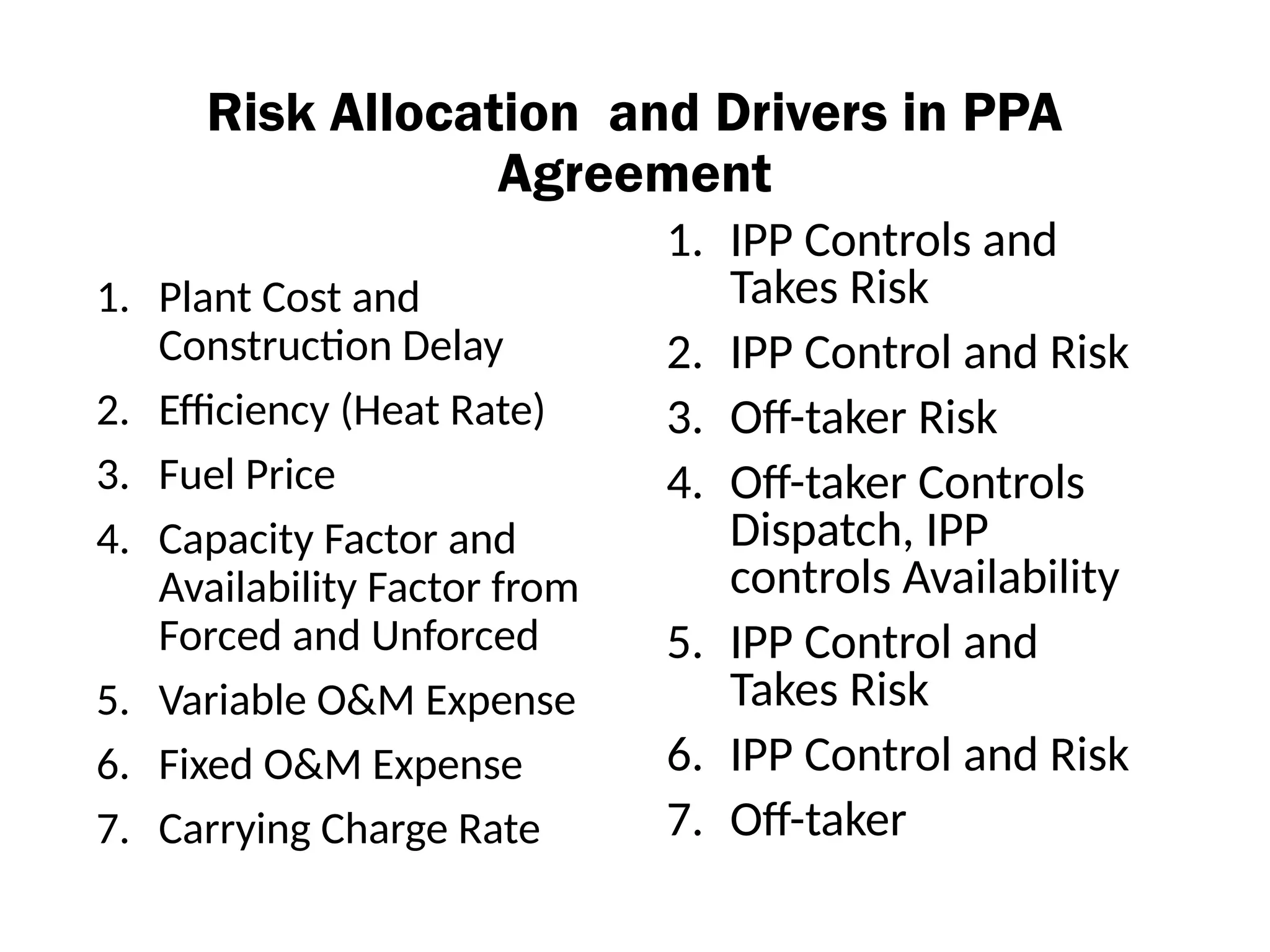
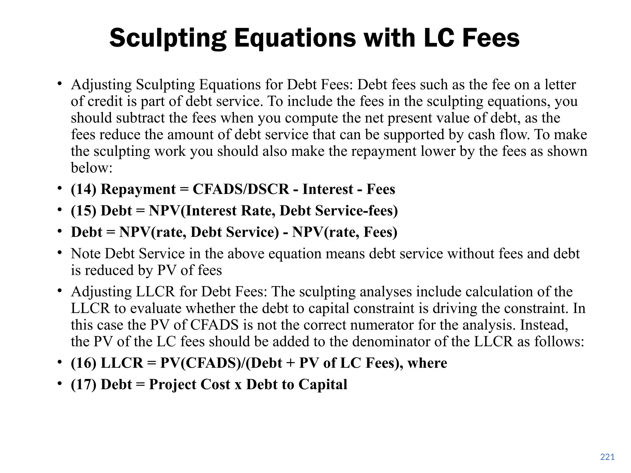
295. • Premium for fixing rates is very expensive
because of expected inflation.
Floating versus Fixed Rate Debt
0.00
1.00
2.00
3.00
4.00
5.00
6.00
7.00
01-août-01
01-janv-02
01-juin-02
01-nov-02
01-avr-03
01-sept-03
01-févr-04
01-juil-04
01-déc-04
01-mai-05
01-oct-05
01-mars-06
01-août-06
01-janv-07
01-juin-07
01-nov-07
01-avr-08
01-sept-08
01-févr-09
01-juil-09
01-déc-09
01-mai-10
01-oct-10
01-mars-11
01-août-11
01-janv-12
01-juin-12
01-nov-12
01-avr-13
01-sept-13
01-févr-14
01-juil-14
01-déc-14
01-mai-15
01-oct-15
01-mars-16
01-août-16
01-janv-17
30
YR
Swap
Rate
30 YR Swap Rate [Final Value 2.07 ] vs
Overnight LIBOR [Final Value 0.43 ]
Overnight LIBOR
30 YR Swap Rate

296. 296
Discussion of Interest and Fees
• Consistent with the discussion of debt as having five
components, interest and fees between the time debt
draws occur and debt is fully repaid is the next topic.
• Interest rates consist of credit spread and base rate.
• Debt IRR is the money the lenders receive including
fees, relative to the amount funded by lenders
• Credit spreads can include step-ups – why they are
present in many transactions and what they mean in
terms of re-financing.
• Loan agreements often require hedging and interest
rate swaps.

297. • Commitment Fee
• (a) The Borrower will: (i) commencing on the date of the first
Utilisation Date until (and including) the last day of the Availability
Period for the borrowing under the Tranche A Facility, pay for a
commitment fee computed at a rate of four per cent. (4%) per
annum on the undrawn and uncancelled portion of the Tranche A
Commitments allocated to the Second Tranche A Loans;
• Commencing on the date of the first Utilisation Date until (and
including) the last day of the Availability Period for the borrowing
of the Second Tranche B Loan under the Tranche B Facility, pay
the Facility Agent for each Lender a commitment fee computed at a
rate of five per cent. (5%) per annum on the undrawn and
uncancelled portion of the
• Tranche B Commitments allocated to the Second Tranche B Loan;
and
Commitment Fee, Up-Front Fee and Debt IRR
297

298. • In the cases without re-financing it seemed that
the credit spread did not make that big a
difference to the equity IRR.
• But when re-financing was included the credit
spread made a big difference as should be
expected – the credit spread is a big driver from
the difference between project IRR and equity
IRR.
• The credit spread is driven by the probability of
default and loss, given default in theory. The
problem is that these statistics are not observable.
Importance of Credit Spreads

299. 299
• NRG Yield presented a table with the margin
earned on interest rates. Most of the project
finance transactions had margins between 2%
and 2.5%. The longest tenor in the table is the
year 2038 implying a remaining term of 23
years.
Example of Interest Rates

300. EXPECTED
LOSS
$$
=
Probability of
Default
(PD)
%
x
Loss Severity
Given Default
(Severity)
%
Loan Equivalent
Exposure
(Exposure)
$$
x
The focus of grading tools is on modeling PD
What is the probability
of the counterparty
defaulting?
If default occurs, how
much of this do we
expect to lose?
If default occurs, how
much exposure do we
expect to have?
Borrower Risk Facility Risk Related
Expected Loss Can Be Broken Down Into Three Components
Credit Spread must cover the expected loss and
is driven by probability of default x loss given
default

301. Comparison of PD x LGD with Precise Formula
-- LGD and Multiple Years
Assumptions
Years 5 BB 5
Risk Free Rate 1 5% 7
Prob Default 1 20.8% PD 20.80%
Loss Given Default 1 80%
Alternative Computations of Credit Spread
Credit Spread 1 3.88%
PD x LGD 1 16.64%
Proof
Opening Closing Value
Risk Free 100 127.63 127.63
Prob Closing Value
Risky - No Default 100 0.95 153.01 145.36
Risky - Default 100 0.05 30.60 1.53
Total Value 146.89 FALSE
Credit Spread Formula
With LGD
cs = ((1+rf)/((1-pd)+pd*(1-lgd))-rf)^(1/years)-1
Formula demonstrating
that Credit spread is
function of PD and LGD
and the risk free rate.
If you are lazy, just use
a goal seek

302. • Use example of 6% and understand compounding of the credit
spread
• For one year if LGD is 50%, then implied PD is about 11.32%
as shown below for a zero coupon bond example.
Implied PD from Credit Spread
302

303. • Like any other interest rate, the credit spread is an IRR
and it compounds dramatically over time. Scenarios with
6% credit spread and 5, 10 and 15 years are shown below.
Implied PD Explodes with Longer Term Debt

304. S&P Study of PD and LGD for Project Finance
There is not much data, but
the data shows that the
LGD is very high for project
finance. This is logical given
the long-term nature of the
assets.

305. Project Finance Defaults
A lot of
merchant
plants in US.
Note the
initial rating of
BBB-

306. S&P Recovery Rates
LGD for
Defaults –
Not much
data

307. Project Finance is Unfair to Africa
Credit spreads are
much higher in
Africa, but compute
the ratio of defaults
to loans.
For U.S. the ratio is
32/21 or 1.53.
For Africa the ratio is
3/8 = .375.

308. Useless but Interesting Chart on PD

309. 309
0
2
4
6
8
10
12
14
16
18
20
1-Sep-97
1-Jan-98
1-May-98
1-Sep-98
1-Jan-99
1-May-99
1-Sep-99
1-Jan-00
1-May-00
1-Sep-00
1-Jan-01
1-May-01
1-Sep-01
1-Jan-02
1-May-02
1-Sep-02
1-Jan-03
1-May-03
1-Sep-03
1-Jan-04
1-May-04
1-Sep-04
1-Jan-05
1-May-05
1-Sep-05
1-Jan-06
1-May-06
1-Sep-06
1-Jan-07
1-May-07
1-Sep-07
1-Jan-08
1-May-08
1-Sep-08
1-Jan-09
1-May-09
1-Sep-09
1-Jan-10
1-May-10
1-Sep-10
1-Jan-11
1-May-11
1-Sep-11
1-Jan-12
1-May-12
1-Sep-12
1-Jan-13
1-May-13
1-Sep-13
1-Jan-14
1-May-14
1-Sep-14
1-Jan-15
1-May-15
1-Sep-15
1-Jan-16
1-May-16
1-Sep-16
Merrill Lynch B Adj Spread Merrill Lynch BB Adj Spread Merrill Lynch BBB Adj Spread Merrill Lynch AAA Adj Spread
#N/A #N/A #N/A #N/A
#N/A #N/A
Target Rating and Credit Spreads – Why the target is BBB- in
Project Finance
Note the spread for
BBB- should be
representative of
Project Finance
BBB and other spreads
were very low prior to
2008 Crisis

310. .00
10.00
20.00
30.00
40.00
50.00
60.00
1 2 3 4 5 6 7 8 9 10 11 12 13 14 15
Default
Rate
(Count)
S&P PD by Credit Rating and Tenure
AAA AA+ AA AA- A+ A
A- BBB+ BBB BBB- BB+ BB
BB- B+ B B- CCC/C
Probability of Default for BBB and Other Ratings
BBB-

311. • You can use the credit spreads along with the PD tables from
S&P to evaluate the IRR earned on different ratings. There are
two scenarios: one where there is no default and another where
the default history by tenure are attributed a loss given default.
The first scenario assumes equal debt service.
Credit Spreads, PD, LGD and RORAC
311
After adjusting for risk, IRR
is much higher for B Spread

312. • In this case, the AA rated spreads from the database are
combined with the default probabilities to evaluate the
risk adjusted IRR from the lower credit spreads. The
risk adjusted IRR now is much smaller than the higher
credit spreads.
Credit Spreads with AA Rated Bonds
312

313. • In this case, the BBB rated spreads from the interest
rate database are combined with the S&P default
probabilities to evaluate the lender risk adjusted IRR
from the lower credit spreads. The risk adjusted IRR
now is much smaller than the higher credit spreads.
Credit Spreads with BBB Rated Bonds which are Proxy for
Project Finance
313

314. • Pre-payments
• If fixed interest rates are in the transaction and rates
are high, the borrower wants pre-payment option
and the lender does not. There can be a set of
defined pre-payment penalties.
• Pre-payments can come from a “divorce” clause
were the borrower pays back the loan instead of
taking some action.
• Maturity Extensions
• If cannot meet the required maturity payments from
cash flow, the loan agreement allow the maturity
payments to be extended
Pre-payments Maturity Extensions from Fixed Rate Debt

315. • Borrower Perspective
• When interest rates decrease, if the loan is at a fixed rate,
the borrower will want to re-finance but the lender will not
want this. Prepayments accelerate (people re-finance).
• Lender Perspective
• From the lenders perspective, the high interest rates are
lost and the lender must issue loans at lower rates. Form
the borrowers perspective, the proceeds will be re-invested
at a lower rate and that bonds will be more expensive.
• The results are like selling a call option for debt
holders -- the upside is limited but the downside is not
limited.
Contraction Risk from Fixed Interest Rates (Declining Interest
Rates)

316. 1-Aug-01
1-Nov-01
1-Feb-02
1-May-02
1-Aug-02
1-Nov-02
1-Feb-03
1-May-03
1-Aug-03
1-Nov-03
1-Feb-04
1-May-04
1-Aug-04
1-Nov-04
1-Feb-05
1-May-05
1-Aug-05
1-Nov-05
1-Feb-06
1-May-06
1-Aug-06
1-Nov-06
1-Feb-07
1-May-07
1-Aug-07
1-Nov-07
1-Feb-08
1-May-08
1-Aug-08
1-Nov-08
1-Feb-09
1-May-09
1-Aug-09
1-Nov-09
1-Feb-10
1-May-10
1-Aug-10
1-Nov-10
1-Feb-11
1-May-11
1-Aug-11
1-Nov-11
1-Feb-12
1-May-12
1-Aug-12
1-Nov-12
1-Feb-13
1-May-13
1-Aug-13
1-Nov-13
1-Feb-14
1-May-14
1-Aug-14
1-Nov-14
1-Feb-15
1-May-15
1-Aug-15
1-Nov-15
1-Feb-16
1-May-16
1-Aug-16
1-Nov-16
1-Feb-17
0.00
1.00
2.00
3.00
4.00
5.00
6.00
7.00
8.00
9.00
10.00
11.00
12.00
10 YR Swap Rate
10 YR Swap Rate
Merrill Lynch BBB Adj Spread
10
YR
Swap
Rate
Total Rate assuming BBB Spread with 10 year Swap Rate
316
Note the low credit
spread before the
financial crisis

317. Example of Pricing and Changing Credit Spreads
Step-up credit spreads encourage re-
financing. To not assume re-financing in
a base case or upside case in
inconsistent with the whole idea of
increasing rates.

318. Part 12: Credit Enhancement: DSRA, MRA,
Cash Flow Sweeps and Covenants

319. • What can you really do if:
• A company does not pay debt service
• A company has a big cost over-run
• There is a big delay in construction
• Answer
• Waiver
• Events of Default
• Failure to Make Payments
• Judgments
• Misstatements
• Cross Default
• Breach of Project Documents
• Breach of Terms of Agreement
• Default in Construction; Schedule (Covenants)
• Loss of Applicable Permits
Default Events and Project Finance Philosophy
319

320. • Possession of Project. Enter into possession of the Project
and perform any and all work and labor necessary:
• to complete the Project substantially according to the EPC
Agreement and
• the Plans and Specifications or to operate and maintain the
Project,
• and all sums expended by Administrative Agent in so
doing, together with interest on such total amount at the
Default Rate, shall be repaid upon demand and
• shall be secured by the Financing Documents,
notwithstanding that such expenditures may, together with
amounts advanced under this Agreement, exceed the
amount of the Total Construction Loan Commitment.
Remedies for Default: Step-in Rights

321. • Cash flow capture (dividend lock-up, cash trap) covenants
• Cause debt to be re-paid early or debt service reserves to be built-up
if debt service coverage ratios are low. Bad time covenant.
• Cash flow sweep covenants
• Cause debt to be re-paid early or debt service reserves to be built-up
if cash flow is high (or low). Good-time covenant.
• Debt service reserves
• Assure debt service can be paid if market prices or other risks cause
cash flow to be low for an extended period of time.
• Subordinated debt and mezzanine finance
• Protects the cash flow coverage of senior debt instruments.
• Contingent equity or sponsor guarantees
• Provide for additional equity funding in downside cases.
Financial Enhancements – Alternative Definition

322. Example of Covenants
• DSCR Target
• Minimum Senior DSCR of 1.20x in Base Case
• Lock-up Covenant
• Minimum Senior DSCR for the previous 12
months to be greater than 1.10x for distribution
• Event of Default
• Minimum Senior DSCR of 1.05x
• Standard Covenant
• Senior Debt not to exceed 80% of the total
project costs

323. • “Distribution Date” means 30 days after
each Repayment Date; provided, however,
that no Distribution Date shall occur prior to
the fourth (4th) Repayment Date.
• Implications and grace period
Dividend Distributions in Solar Case
323

324. • Covenants cannot increase the operating cash
flow of a project
• Covenants cannot make a project that does not
have enough cash flow to avoid default
• Covenants cannot make a bad project into a
good project
• Covenants can change the timing of dividends
• Covenants and DSCR can force liquidity into
a project
What Covenants Cannot and Can Do

325. • The timing of debt service (i.e. loan interest payments and
principal repayments) is one of the biggest factors that
drives the rate of return for equity holders in a project. If
the debt service is structured to allow no dividends until all
debt is paid, return will be lower. This will generally be
unacceptable to sponsors.
• The faster investors in a project are paid dividends, the better
their rate of return.
• Investors therefore do not wish cash flow from operations of the
project to be devoted to lenders at the expense of these
dividends.
• Lenders, on the other hand, generally wish to be repaid as
rapidly as possible. Striking a reasonable balance between these
conflicting demands is an important part of loan negotiations.
Investors Need Some Dividends Before All Debt is Paid Off

326. • The most important aspect of the underwriting process is determining
whether the plant is economically sound. This means that the cost
structure and the technology of the plant must be viable.
• However, once a plant is determined to be economically viable, the
credit quality of a transaction can be enhanced by various structural
features – covenants, debt service reserves, liquidation damages,
subordinated debt, contingent equity etc. The potential for structural
enhancements to improve the credit quality of a transaction is
described in the statement by Standard and Poor’s below:
• Project structure does not mitigate risk that a marginally economic project
presents to lenders; structure in and of itself cannot elevate the debt rating of
a fundamentally weak project to investment-grade levels. On the other hand,
more creditworthy projects will feature covenants designed to identify
changing market conditions and trigger cash trapping features to project
lenders during occasional stress periods.
Covenants and Structural Enhancements Cannot Make a Bad
Project into a Good Project

327. • A cash flow waterfall defines the priority
of uses of cash flow that is received for a
project.
• The important part of a cash flow
waterfall is what happens if there is not
enough cash flow to pay all expenses,
debt service and debt service reserve
requirements. It is the area after senior
debt payments and before dividends
• If sufficient cash is available to pay
dividends, the cash flow priority defines
how and when a distribution can be made.
Covenants and Cash Flow Waterfall

328. • Set-up Cash Flow Working from EBITDA to CFADS
• Take away senior debt service assuming that debt
service is paid
• Use a lot of sub-totals for cash flow after debt
service, cash flow before default, cash flow before
use of DSRA etc.
• Use MAX(number,0) or Max(-number,0) to test for
what to do when sub-total is positive or negative
• Use MIN(subtotal, opening balance) to limit the
amount of sweep, DSRA use, repayment of default
etc.
Modelling of Cash Flow Waterfall
328

329. • All revenues accrued on and after the Commercial Operation
Date will be deposited with the Trustee into the Operating
Revenue Account. The Trustee will withdraw amounts on a
monthly basis and make deposits in the following priority, but
only to the extent funds are then available in the Operating
Revenue Account:
• (1) the operations and maintenance expenses for the Project for such month,
subject to certain limitations;
• (2) the Tax Equalization Account
• (3) (A) an amount that will not be less than the amount of interest on the Bonds to
become due on such Interest Payment Date, and (B) an amount that will not be less
than the amount of principal or sinking fund payment to become due on such
principal or sinking fund payment date;
• (4) an amount, if any, sufficient to cause the amount on deposit in the Debt Service
Reserve Account to equal the Debt Service Reserve Account Requirement;
• (5) an amount, if any, sufficient to pay amounts due pursuant to the Working
Capital Facility;
• (6) an amount equal to the balance of the Operating Revenue Account shall be
deposited into the Surplus Account and will be transferred monthly to the
Operating Revenue Account.
Example of Cash Flow Priority

330. • Amounts in the Surplus Account will be annually
transferred on the first business day of January to the
Distribution Account and distributed to the Partnership
within 90 days thereafter if:
• the Debt Service Coverage Ratio for the Project is equal to
or exceeds 1.20 to 1.00 for the calendar year preceding the
distribution date and is projected to be equal to or exceed
1.20 to 1.00 for the current calendar year;
• the Partnership does not have knowledge, or could not
reasonably be expected to have knowledge, of the
occurrence and continuance of an event of default …;
• Working Capital Facility and the Waste Supply Support
Facility have been fully restored.
• If not so distributed, amounts in the Distribution
Account shall revert to the Surplus Account.
Example of Lock-up and Cash Flow

331. • Cash Lock-up (dividend lock-up, cash trap) is a “bad time” covenant.
It stops dividends when there is not much cash left anyway.
• Cash lock-up – if things are getting bad, do not allow dividends and try
to get a little more protection for things getting even worse.
• Program lock-ups from historic DSCR with a switch variable.
Prospective lock-ups cause a circular reference that is probably not
worth solving.
• Cash sweeps can be though of as a “good time” covenant. They can
limit dividends when there is a lot of cash available and protect the
lender for later periods when there is less cash.
• Cash sweeps are programmed with MAX/MIN functions and sub-totals
• MAX so the sweep occurs only when cash flow is positive
• MIN to make sure you do not sweep too much cash flow
• It would not make sense to have some formula for a cash sweep that
prepays debt when some low level of DSCR occurs – this is redundant
with the lock-up. Ratios like Debt/EBITDA make work better.
Theory of Lock-up and Cash Flow Sweep

332. • A cash sweep covenant only makes sense in
situations where the cash flow is volatile and/or there
are potential downward trends in prices.
• Think about a sudden 2008 type decline in cash flow.
Lenders do not like to have paid dividends only to later
have a default
• If cash flow is always low there is no cash flow to sweep
anyway. Here the sweep will not help.
• If cash flow is always high, there is no need for the cash
sweep.
• To assess the effectiveness of the covenant, cases that
incorporate realistic price volatility and potential
price trends must be run in the model.
Volatility and Risk Reduction from Cash Flow Sweeps

333. Example of Risk and Return Analysis for Cash Flow Sweep
Sweeps really help when there is a sudden decline in
cash flow – when you would have paid dividends
otherwise. A sweep would have reduced the default in
the example below.
Dividends
Default
Default
Repayment of
default

334. 334
Economic and Financial Analysis of Cash Sweeps, Reserve
Accounts and Covenants
• Cash sweeps, reserve accounts and covenants can have
negative effects on the equity IRR of a project.
• Methods to consider the risk benefits to the bank versus the
costs to sponsors are addressed.
• Mechanics of cash sweep with different triggers and theory of
what kinds of transactions would be relevant for cash sweep
(e.g. hydro but not solar because of volatility) are addressed.
• The theory of what kind of triggers make sense
(Debt/EBITDA but not DSCR and operational triggers).
• Contrast between cash sweeps and cash trap covenants. As
with other issues, the effects of cash sweeps on equity returns
should be addressed with and without re-financing
assumptions.

335. 335
Importance of Re-financing Analysis with Cash Sweep
• Cash Sweeps seem to dramatically reduce the
cash flow
• But after the prepayments from the sweep (or
even before), the project can be re-financed
• You can even lock-in interest rates if you are
worried about interest rate risk.
• Again, re-financing changes everything – you
can get you super dividends when you re-
finance.

336. • The Borrower may, prepay any Tranche B Loan at
any time in whole or in part, which
• (i) after the Tranche A Loans and all Obligations in
relation thereto have been unconditionally and
irrevocably repaid and paid in full,
• and (ii) prior thereto will be applied
• (A) first, to pay any accrued but unpaid interest that
has not yet been paid in kind and
• (B) second, to repay such portion of the principal
amount outstanding of the Tranche B Loans, if any, that
is equal to the remaining portion of the prepayment
amount on the date of prepayment.
Prepayment in Airport Case
336

337. Debt Service Reserve Accounts

338. • Cost of Debt Service Reserve Account compared
to benefits
• Who funds the debt service reserve account, debt
or equity or debt and equity
• Mechanics and theory of using and L/C for the
debt service reserve account and support of parent
• Measuring the benefits of using an L/C account
compared to a funded DSRA with different
scenarios
• Effect of L/C fees in O&M expense versus L/C
fees as part of debt service
Theory of DSRA
338

339. • DSRA is built to get liquidity into the project because holding
cash is very expensive – often 6 months of debt service which
is arbitrary
• Return on cash is about zero and opportunity cost of funds is equity
or debt IRR
• You can sometimes use a letter of credit instead of cash.
• Letter of credit should have a parent guarantee
• Paying an LC fee costs much less than the opportunity cost of funds
• If debt size is driven by the DSCR and not the debt to capital,
then the DSRA is funded by equity and not debt. This is
because the level of debt is given.
• If the debt to capital is high and the equity contribution is low,
the DSRA can be very costly to the equity IRR because of
high debt service and low equity.
DSRA and Liquidity

340. • Bankers should not care if the DSRA is
funded by debt or equity – the idea is just to
have liquidity when temporary bad things
happen or to have time to restructure.
• You can make the last repayment the DSRA.
In this case, with sculpting, the amount of the
cash flow increases and the debt also
increases. This has a small positive effect on
the equity IRR as shown in the next slide.
Using the DSRA as the Final Repayment in Sculpting
340

341. • The example below shows the effect of using the DSRA in
sculpting debt. The left hand side includes DSRA and the right
hand side does not. Without DSRA the IRR is 12.65%.
Example Using the DSRA as the Final Repayment in Sculpting
341

342. • The example below shows that with a high debt to
capital ratio driven by sculpting and a high IRR,
the DSRA in LC can make a big difference to the
equity IRR – 11.96% to 14.92% as shown below.
Use of LC Instead of the DSRA
342

343. • “Acceptable DSR Letter of Credit”
• issued by a financial institution whose long-term senior unsecured debt is
rated at least “A-” by S&P and “A3” by Moody’s,
• naming Administrative Agent on behalf of the Lenders as the beneficiary, and
• including provisions that
• (i) such letter of credit shall automatically renew upon the expiration
• (ii) if no agreement for a renewal or replacement of the letter of credit has been
made after the long-term senior unsecured debt rating of the financial institution
that provides the letter of credit is downgraded below “A-” by S&P or “A3” by
Moody’s, the stated amount of the letter of credit shall be automatically drawn and
the proceeds automatically deposited in the Debt Service Reserve Account.
• Letter of credit
• (A) shall have an initial expiration date of at least one year after issuance,
• (B) shall not impose on Borrower any obligation to reimburse drawing payments,
and
• (C) shall be issued in a face amount equal to amounts required to be retained in the
Debt Service Reserve Account.
DSRA as LC in Solar Case
343

344. • The Borrower must ensure that, on the first Utilisation Date, the balance of the
Debt Service Reserve Account is US$5,000,000. On each Monthly Transfer Date
thereafter, the Borrower must ensure that the balance in the Debt Service
Reserve Account is an amount equal to US$5,000,000
• or, if a Funds Insufficiency has occurred and the Borrower or the Facility Agent has
applied monies from the Debt Service Reserve Account to cover such Funds
Insufficiency, an amount equal to: (i) if the balance in the Debt Service Reserve
Account is less than US$3,000,000, the amount equal to the difference between
US$3,000,000 and the amount then on deposit in the Debt Service Reserve Account
the sum of (x) three million US Dollars (US$3,000,000), plus (y) the aggregate amount
of transfers made from the Collection Account to the Debt Service Reserve Account,
which transfers the Borrower must ensure, in accordance with agree to or propose any
major adjustment or increment request on design standard and/or structure or
otherwise or any material change on bills of quantities, contract value or construction
period, or otherwise vary, modify, supplement or amend or agree to the variation,
modification, supplementation or amendment in any way of any material provision of
either China Civil Engineering Construction Contract of the performance of any
material obligation by any other Person under such China Civil Engineering
Construction Contract, in each case by entry into a supplementary agreement or
otherwise; provided that the Facility Agent will not unreasonably withhold its consent
to any of the foregoing if such consent is requested by the Borrower;
Debt Service Reserve Account in Airport Case
344

345. • On the Closing Date, an amount equal to 10% of the original principal amount
of the Bonds will be deposited in the Debt Service Reserve Account of the Debt
Service Reserve Fund from the proceeds of the Bonds.
• The amounts in the Debt Service Reserve Account will be used only for the
purpose of making payments into the related Interest Subaccounts, the Principal
Subaccounts and Sinking Fund Installment Subaccounts for the Bonds
• If a disbursement is made under a Debt Service Reserve Account Facility, the
Trustee shall apply amounts transferred from the Operating Revenue Account to
the applicable Debt Service Reserve Account to either cause the reinstatement of
the maximum limits of such Debt Service Reserve Account Facility. The Trustee
will apply moneys on deposit in a Debt Service Reserve Account prior to any
drawing on any Debt Service Reserve Account Facility.
• In the event that any amount shall be withdrawn from a Debt Service Reserve
Account for payments into an Interest Subaccount, Principal Subaccount or
Sinking Fund Installment Subaccount or there exists a deficiency in a Debt
Service Reserve Account which is to be reinstated, such withdrawals shall be
subsequently restored from Revenues available on a pro rata basis after all
required payments have been made into such Interest Subaccount.
Debt Service Reserve Language

346. • Accounts
• Airport Case
• Revenue Account means the bank account
no. 4603 held in the name of the Borrower
into which all Revenues of the Borrower,
other than those deposited into the Collection
Account are deposited.
Case Flow Waterfall
346

347. • Accounts. On or prior to the Closing Date, Borrower and Administrative Agent
shall establish at the Depositary accounts entitled
• “Solar Construction Account” (the “Construction Account”),
• “Solar Operating Account” (the “Operating Account”),
• “Solar Distribution Account” (the “Distribution Account”),
• “Solar O&M Reserve Account” (the “O&M Reserve Account”),
• “Solar Debt Service Reserve Account” (the “Debt Service Reserve Account”),
• “Solar Distribution Reserve Account (the “Distribution Reserve Account”),
• “Solar Completion Reserve Account” (the “Completion Reserve Account”),
• “Solar Interest Reserve Account” (the “Interest Reserve Account”)
• “Solar Loss Proceeds Account” (the “Loss Proceeds Account”),
• “Solar Delay Proceeds Account” (the “Delay Proceeds Account”)
• “Solar Major Maintenance Reserve Account” (the “Major Maintenance Reserve
Account”).
• Any deposits, transfer or application of funds in the Accounts shall be in
accordance with the Depositary Agreement.
Solar Case Accounts
347

348. Section 8: Re-financing and effects of
Debt Tenure (as well as other debt terms)

349. • Assume that the debt is sized from debt to capital
ratio for the next set of slides (this assumption
will be changed later on)
• Assume that the debt can be re-financed on the
basis of DSCR (this assumption will also be
changed in later slides).
• Various assumptions will be made about re-
financing
• The slides will demonstrate that with these
assumptions, re-financing makes the length of the
debt much less important.
Re-financing and the Importance of Debt Tenure

350. • Every project has the possibility to increase equity
returns through re-financing
• Re-financing is a real option without a cost if there is
no pre-payment penalty (except for fees on new debt)
• As with any option, the value of the option is driven
by uncertainty – there is uncertainty with respect to
when the re-financing occurs, the parameters of the
re-financing, the credit spreads and the amount of the
re-financing
• The re-financing option has much much more value
when the initial tenor is short.
Re-financing Introduction
350

351. • The excerpts below show the assumptions
and the mechanics behind re-financing
Assumptions and Mechanics of Re-financing

352. • The table below illustrates alternative re-financing
scenarios using the assumption of DSCR driving
the debt size in re-financing. Results of these
sensitivities are presented in subsequent slides.
This kind of table should be in every model
Re-financing Scenarios

353. • If there are multiple re-financings, the effect
of the tenure on the IRR is dramatically
reduced as shown in the two tables below.
Re-financing Case 1 – Multiple Re-financings

354. • An argument against the dramatic effects of re-
financing is that the length of the debt is a very strong
signal – like a stamp of approval – that the project has
reasonable risk.
• If one project obtains an advantageous financing at the
financial close, why would the project not also receive
better terms in re-financing.
• If the short tenure is just a reflection of market
conditions in a country or the necessity to establish
historic results.
• There are many possibilities about how re-financing
could occur and sensitivity analysis can be performed.
Philosophy and Re-financing

355. • This scenario shows that if the re-financing occurs later
there is a smaller effect because higher dividends occur
in early years. The table shows Equity IRR
Re-financing Case 2 – Later Refinancing

356. • This scenario demonstrates that if the re-
financing occurs later but there is a longer tenure
for the re-financing then the effect is increased.
Re-financing Case 3 – Shorter Tail in Re-financing

357. • The scenario with reduced interest and
reduced DSCR demonstrates higher returns
in all scenarios.
Re-financing Case 4 – Reduced DSCR and Interest Rate on
Re-financing

358. • When re-financing is included interest rate changes make a big
difference and loan tenor is much less important. If you believe that
you can re-finance, it is more important to negotiate a low interest rate.
Re-financing Case 5 – Effect of Interest Rates when Re-
financing Included

359. • When re-financing is included and the interest rate is reduced on future
financing and the DSCR is reduced, the re-financing effects are more
dramatic. The gearing makes more difference and the initial tenor has
a smaller effect.
Re-financing Case 6 – Effect of Changing Interest
Rates and DSCR for Sizing Re-financing

360. • Not being “allowed” to consider re-financing
is silly.
• Consider a variety of re-financing
possibilities with scenario analysis
• Re-financing can dramatically change the
implications of interest rates and tenures.
• Re-financing a particularly important issue
for cases where the loan tenure is a lot shorter
than the project life.
Re-financing Conclusions

361. Part 14: Other Project Finance Subjects: IRR
problems, Risk and Value Changes over Life of
Project, Resource Analysis and Debt Sizing

362. 362
• Valuation theory with respect to projects generally involves risk reduction as a
project progresses through phases.
• In Europe, there are many stories (but not much data) about how insurance
companies purchase existing projects with operating history and are willing to
accept equity IRR’s as low as 5-6%.
• The idea behind a low cost of capital for mature projects is the following:
• During the development stage, expenditures occur with large risks associated with permitting,
problematic wind studies, construction cost over-runs, ability to secure tariffs etc. The
required equity IRR during the development stage can be 15% to account for the project not
being successfully methods.
• Once the development is finished or in late stages, the risk is reduced by a large margin.
However there are still risks associated with successfully completing construction at budget
and on time. The reduced risk during the construction phase may reduce the required equity
IRR to something like 12%
• After construction, the remaining risk for a project with a fixed price contract is that the
estimated wind production will not be met. Given this risk, the discount risk is still above the
cost of capital for bonds and may be in the range of 8-10%.
• Once operating history is available, the risk is not much higher than the debt cost or the
interest rate on long-term bonds. With bonds yielding below 3%, a return of 6% provides a
good premium for risk.
A Little Theory about Valuation and Risk of Projects

363. 363
Re-financing and Early Project Sale
• Timing strategies and sales value. How
different types of projects have differences in
risk reduction over time, and why wind
projects probably have more of a risk
reduction than other electricity projects. Show
how the effects of changing risk and selling to
a Yieldco can be demonstrated with
measuring IRR over time with changing buyer
IRRs. Demonstrate how optimal holding
periods can be computed with various IRR
hurdle rate assumptions.

364. 364
• As part of this task we have reviewed detailed financial data of
Yieldco’s including prospectuses and annual financial reports. One of
the last companies that we investigated was Brookfield Renewable
Energy Partners (BEP). In its notes to financial statements, discount
rates that are applied to both contractual cash flows and non-
contracted cash flows in asset valuation are presented. It is assumed
that the cost of capital represents after tax cost of capital although
this is not specified in the report.
Verification of Cost of Capital from Published Data in Yieldco
Reports

365. Equity Returns and Re-Financing
7.8%
29.2%
37.3%
44.6%
7.7%
16.0%
18.9%
21.7%
0.0%
5.0%
10.0%
15.0%
20.0%
25.0%
30.0%
35.0%
40.0%
45.0%
50.0%
Low Base High Very High
E
q
u
i
t
y
I
R
R
Traffic Scenario
Equity IRR with and without Re-financing
Re-Finance
No Re-Finance

366. 366
• For valuation of assets the most relevant multiple is the EV/EBITDA
ratio. This is because the EBITDA is not affected by financing and
because the EV/EBITDA ratio can be computed from IPO’s of
Yieldco’s. For Yieldco projects that have minimal capital expenditures
and small or no growth in cash flow, the EV/EBITDA can be used to
derive an implied pre-tax IRR and an overall cost of capital (this is
further explained in the appendix). The IRR’s from this analysis are
lower than the low case pre-tax cost of capital assumption.
Transaction Multiples from Yieldco IPO’s

367. Equity Returns for Tollroads
• The following slide shows equity returns over time
and how they have come down

368. Part 3: Creating or Destroying Value through
Contract Provisions Including Liquidated Damages,
Penalty Provisions and Efficiency Incentives

369. • Begins with Project Contract (Concession
Contract, PPA Contract, Availability Contract).
• Back to back contracts follow the Project
Contract
• Fixed Price EPC Contract from Fixed
Availability Payment
• Transfer Delay Risk with Liquidated Damage
• Transfer O&M Risks with Incentives and
Penalties
General Notion of Back to Back Contacts
369

370. • Notion of allocating risks to IPP that can be controlled
• Incorporation of different risks in multipart tariffs
• The general idea that risks which can be accepted at a
reasonable cost should be allocated to IPP versus the
off-taker.
• Nuances of whether risks should be allocated.
• Notion that penalties and bonuses should reflect off-
taker costs combined with SPV costs
• Use of marginal cost analysis in measuring availability
benefits and costs in different periods
• Calculation levelized prices in PPA contracts
Economic Efficiency of Contracts in Project Finance
370

371. Example of Delay Damage in PPA Contract
371

372. Example of Delay LD in EPC Contract
372

373. 373
Theory of Risk and Return in Project Finance
• Different parties in project finance including EPC contractors,
O&M contractors, insurance companies, financial institutions
and sponsors are paid for taking risk.
• The general idea that if parties are paid too much or too little
for accepting risk, the off-taker will pay too much for the
service and/or sponsors will not receive an adequate return
will be demonstrated.
• Off-taker economics as well as the technical aspects of the
facility must be fully understood to effectively negotiate
project finance terms.
• The theory and practice of computing delay liquidated
damages, availability penalties, target heat rates and other
items through the central idea of minimizing the sum of off-
taker costs and IPP costs.

374. Special
Purpose
Vehicle
Off-taker
PPA Contract
Four Part Tariff
Fixed Capacity Charge at Fin Close
LD Penalty for Delay Risk
Contract O&M Charge
Contract Heat Rate
Availability Penalty
EPC
Contractor
Fixed Price
Contract with LD
O&M
Contractor
Contract with
Guaranteed Heat
Rate and Availability
Penalty
and Fixed Fee
Fuel Supply
Fuel Index
Lenders
Sponsors
Fuel Supply Contract
with Index
Corresponding to
PPA
Loan
Agreement
Shareholder
Agreement
Letter of
Credit for
Equity Cash
Contracts

375. Example of O&M Contract

376. Tradeoff Between Cost and Availability

377. Optimisation and Minimum Cost
In Theory, Minimum is
where replacement cost
change = maintenance
cost change