The document discusses techniques for virtual data integration and transformation as well as the role of data warehouses in master data management. It emphasizes the benefits of a centralized database for improved performance and data governance, detailing the use of ETL tools for extracting, transforming, and loading data. Additionally, it explores the evolving landscape of data integration with hybrid approaches, including the use of MapReduce for querying large datasets.

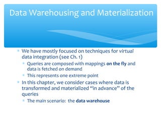
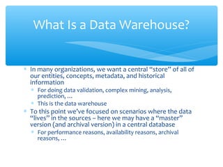
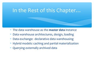
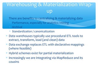
2. +919892900103 |
info@vibranttechnologies.co.in
| www.
Vibranttechnologies.co.in
Contact us on :

3. ∗ We have mostly focused on techniques for virtual
data integration (see Ch. 1)
∗ Queries are composed with mappings on the fly and
data is fetched on demand
∗ This represents one extreme point
∗ In this chapter, we consider cases where data is
transformed and materialized “in advance” of the
queries
∗ The main scenario: the data warehouse
Data Warehousing and Materialization

4. ∗ In many organizations, we want a central “store” of all of
our entities, concepts, metadata, and historical
information
∗ For doing data validation, complex mining, analysis,
prediction, …
∗ This is the data warehouse
∗ To this point we’ve focused on scenarios where the data
“lives” in the sources – here we may have a “master”
version (and archival version) in a central database
∗ For performance reasons, availability reasons, archival
reasons, …
What Is a Data Warehouse?

5. ∗ The data warehouse as the master data instance
∗ Data warehouse architectures, design, loading
∗ Data exchange: declarative data warehousing
∗ Hybrid models: caching and partial materialization
∗ Querying externally archived data
In the Rest of this Chapter…

6. The data warehouse
∗ Motivation: Master data management
∗ Physical design
∗ Extract/transform/load
∗ Data exchange
∗ Caching & partial materialization
∗ Operating on external data
Outline

7. ∗ One of the “modern” uses of the data warehouse is not
only to support analytics but to serve as a reference to all
of the entities in the organization
∗ A cleaned, validated repository of what we know
… which can be linked to by data sources
… which may help with data cleaning
… and which may be the basis of data governance (processes
by which data is created and modified in a systematic way,
e.g., to comply with gov’t regulations)
∗ There is an emerging field called master data management
out the process of creating these
Master Data Management

8. Data Warehouse Architecture
∗ At the top – a centralized
database
∗ Generally configured for
queries and appends – not
transactions
∗ Many indices, materialized
views, etc.
∗ Data is loaded and
periodically updated via
Extract/Transform/Load
(ETL) tools
Data Warehouse
ETL ETL ETL ETL
RDBMS1 RDBMS2
HTML1 XML1
ETL pipeline
outputs
ETL

9. ∗ ETL tools are the equivalent of schema mappings in virtual
integration, but are more powerful
∗ Arbitrary pieces of code to take data from a source,
convert it into data for the warehouse:
∗ import filters – read and convert from data sources
∗ data transformations – join, aggregate, filter, convert data
∗ de-duplication – finds multiple records referring to the same
entity, merges them
∗ profiling – builds tables, histograms, etc. to summarize data
∗ quality management – test against master values, known
business rules, constraints, etc.
ETL Tools

10. Example ETL Tool Chain
∗ This is an example for e-commerce loading
∗ Note multiple stages of filtering (using selection or join-like
operations), logging bad records, before we group and load
Invoice
line items
Split
Date-
time
Filter
invalid
Join
Filter
invalid
Invalid
dates/times
Invalid
items
Item
records
Filter
non -
match
Invalid
customers
Group by
customer
Customer
balance
Customer
records

11. ∗ Two aspects:
∗ A central DBMS optimized for appends and querying
∗ The “master data” instance
∗ Or the instance for doing mining, analytics, and prediction
∗ A set of procedural ETL “pipelines” to fetch, transform, filter,
clean, and load data
∗ Often these tools are more expressive than standard
conjunctive queries (as in Chapters 2-3)
∗ … But not always!
This raises a question – can we do warehousing with declarative
mappings?
Basic Data Warehouse – Summary

12. The data warehouse
Data exchange
∗ Caching & partial materialization
∗ Operating on external data
Outline

13. ∗ Intuitively, a declarative setup for data warehousing
∗ Declarative schema mappings as in Ch. 2-3
∗ Materialized database as in the previous section
∗ Also allow for unknown values when we map from
source to target (warehouse) instance
∗ If we know a professor teaches a student, then there
must exist a course C that the student took and the
professor taught – but we may not know which…
Data Exchange

14. A data exchange setting (S,T,M,CT) has:
∗ S, source schema representing all of the source tables
jointly
∗ T, target schema
∗ A set of mappings or tuple-generating dependencies
relating S and T
∗ A set of constraints (equality-generating dependencies)
Data Exchange Formulation
(∀X)s1(X1), ..., sm (Xm ) → (∃Y) t1(Y1), ..., tk (Yk )
)Y(Y)Y(t...,,)Y()tY( jill11 =→∃

15. An Example
Source S has
Teaches(prof, student)
Adviser(adviser, student)
Target T has
Advise(adviser, student)
TeachesCourse(prof, course)
Takes(course, student)
),(),,(.,),(:
),(),(:
),(),,(.),(:
),(.),(:
4
3
2
1
studCTakesCDrseTeachesCouDCstudprofAdviserr
studprofAdvisestudprofAdviserr
studCTakesCprofrseTeachesCouCstudprofTeachesr
studDAdviseDstudprofTeachesr
∃→
→
∃→
∃→
existential variables represent unknowns

16. ∗ The goal of data exchange is to compute an instance
of the target schema, given a data exchange setting D
= (S,T,M,CT) and an instance I(S)
∗ An instance J of Schema T is a data exchange solution
for D and I if
1. the pair (I,J) satisfies schema mapping M, and
2. J satisfies constraints CT
The Data Exchange Solution

17. Instance I(S) has
Teaches
Adviser
prof student
Ann Bob
Chloe David
Back to the Example, Now with Data
adviser student
Ellen Bob
Felicia David
adviser student
Ellen Bob
Felicia David
course student
C1 Bob
C2 David
prof course
Ann C1
Chloe C2
Instance J(T) has
Advise
TeachesCourse
Takes
variables or labeled nulls
represent unknown values

18. Instance I(S) has
Teaches
Adviser
prof student
Ann Bob
Chloe David
This Is also a Solution
adviser student
Ellen Bob
Felicia David
adviser student
Ellen Bob
Felicia David
course student
C1 Bob
C1 David
prof course
Ann C1
Chloe C1
Instance J(T) has
Advise
TeachesCourse
Takes
this time the labeled
nulls are all the same!

19. ∗ Intuitively, the first solution should be better than the
second
∗ The first solution uses the same variable for the course
taught by Ann and by Chloe – they are the same course
∗ But this was not specified in the original schema!
∗ We formalize that through the notion of the universal
solution, which must not lose any information
Universal Solutions

20. First we define instance homomorphism:
∗ Let J1, J2 be two instances of schema T
∗ A mapping h: J1  J2 is a homomorphism from J1 to J2 if
∗ h(c) = c for every c ∈ C,
∗ for every tuple R(a1,…,an) ∈ J1 the tuple R(h(a1),…,h(an)) ∈ J2
∗ J1, J2 are homomorphically equivalent if there are homomorphisms
h: J1  J2 and h’: J2  J1
Def: Universal solution for data exchange setting
D = (S,T,M,CT), where I is an instance of S.
A data exchange solution J for D and I is a universal solution if, for
every other data exchange solution J’ for D and I, there exists a
homomorphism h: J  J’
Formalizing the Universal Solution

21. ∗ The standard process is to use a procedure called the chase
∗ Informally:
∗ Consider every formula r of M in turn:
∗ If there is a variable substitution for the left-hand side (lhs) of r
where the right-hand side (rhs) is not in the solution – add it
∗ If we create a new tuple, for every existential variable in the
rhs, substitute a new fresh variable
∗ See Chapter 10 Algorithm 10 for full pseudocode
Computing Universal Solutions

22. ∗ Universal solutions may be of arbitrary size
∗ The core universal solution is the minimal universal
solution
Core Universal Solutions

23. ∗ As with the data warehouse, all queries are directly posed
over the target database – no reformulation necessary
∗ However, we typically assume certain answers semantics
∗ To get the certain answers (which are the same as in the
virtual integration setting with GLAV/TGD mappings) –
compute the query answers and then drop any tuples with
labeled nulls (variables)
Data Exchange and Querying

24. ∗ From an external perspective, exchange and
warehousing are essentially equivalent
∗ But there are different trade-offs in procedural vs.
declarative mappings
∗ Procedural – more expressive
∗ Declarative – easier to reason about, compose, invert,
create matieralized views for, etc. (see Chapter 6)
Data Exchange vs. Warehousing

25. The data warehouse
Data exchange
Caching & partial materialization
∗ Operating on external data
Outline

26. ∗ Many real EII systems compute and maintain materialized views,
or cache results
A “hybrid” point between the fully virtual and fully materialized
approaches
The Spectrum of Materialization
Virtual integration
(EII)
Data exchange /
data warehouse
sources materialized all mediated relations
materialized
caching or partial materialization –
some views materialized

27. Cache results of prior queries
∗ Take the results of each query, materialize them
∗ Use answering queries using views to reuse
∗ Expire using time-to-live… May not always be fresh!
Administrator-selected views
∗ Someone manually specifies views to compute and maintain,
as with a relational DBMS
∗ System automatically maintains
Automatic view selection
∗ Using query workload, update frequencies – a view
materialization wizard chooses what to materialize
Possible Techniques for Choosing
What to Materialize

28. The data warehouse
Data exchange
Caching & partial materialization
Operating on external data
Outline

29. ∗ Many Web scenarios where we have large logs of data
accesses, created by the server
∗ Goal: put these together and query them!
∗ Looks like a very simple data integration scenario –
external data, but single schema
∗ A common approach: use programming environments like
MapReduce (or SQL layers above) to query the data on a
cluster
∗ MapReduce reliably runs large jobs across 100s or 1000s of
“shared nothing” nodes in a cluster
Many “Integration-Like” Scenarios
over Historical Data

30. ∗ MapReduce is essentially a template for writing distributed
programs – corresponding to a single SQL
SELECT..FROM..WHERE..GROUP BY..HAVING block with
user-defined functions
∗ The MapReduce runtime calls a set of functions:
∗ map is given a tuple, outputs 0 or more tuples in response
∗ roughly like the WHERE clause
∗ shuffle is a stage for doing sort-based grouping on a key
(specified by the map)
∗ reduce is an aggregate function called over the set of tuples
with the same grouping key
MapReduce Basics

31. 31
MapReduce Dataflow “Template”: Tuples  Map
“worker”  Shuffle  Reduce “worker”
Map
Worker
Map
Worker
Map
Worker
Map
Worker
Reduce
Worker
Reduce
Worker
Reduce
Worker
Reduce
Worker
Reduce
Worker
emit tuples
emit aggregate
results

32. ∗ Some people use MapReduce to take data, transform it, and
load it into a warehouse
∗ … which is basically what ETL tools do!
∗ The dividing line between DBMSs, EII, MapReduce is blurring as
of the development of this book
∗ SQL  MapReduce
∗ MapReduce over SQL engines
∗ Shared-nothing DBMSs
∗ NoSQL
MapReduce as ETL

33. ∗ There are benefits to centralizing & materializing data
∗ Performance, especially for analytics / mining
∗ Archival
∗ Standardization / canonicalization
∗ Data warehouses typically use procedural ETL tools to
extract, transform, load (and clean) data
∗ Data exchange replaces ETL with declarative mappings
(where feasible)
∗ Hybrid schemes exist for partial materialization
∗ Increasingly we are integrating via MapReduce and its
cousins
Warehousing & Materialization Wrap-
up

34. Thank you