このスライドは http://kazunorisakai.com/ でも公開しています。

1. PRML 2.4 指数型分布族
5501 酒井⼀徳
10/11/17

2. 目次
2.4 指数型分布族
• 2.4.1 最尤推定と⼗分統計量
• 2.4.2 共役事前分布
• 2.4.3 無情報事前分布

3. <latexit sha1_base64="BWB9IVpNwEL+vV2Y0EHq4a+x7jI=">AAADX3ichVG7btRAFL1eAwkBEgMNiGaU1aKkWY0jJBASUiQkRAWbxyaR4rCyveO1Fb9kj5csZn+AH6CgAokC8Qe0FPADFCkpUcog0VBwPGuJxwYYyzNnzr3nPuY6aRjkkvNDraGfOn1mZvbs3LnzF+YXjIuXtvKkyFzRdZMwyXYcOxdhEIuuDGQodtJM2JETim1n/25l3x6KLA+SeFOOUrEX2YM48ALXlqB6xruULTErsqXveKxkB2zMnjLLScJ+PopwgLOEtEEvszvMn3JeZoOKO1lgiYOUWaHwpFWe7POoglXALALaBDP+JUGB23RCKwsGvrTGPaPJ21wtNg3MGjSpXp3E+EAW9SkhlwqKSFBMEjgkm3J8u2QSpxTcHpXgMqBA2QWNaQ7aAl4CHjbYfewD3HZrNsa9ipkrtYssIf4MSkYt/om/4cf8I3/Lv/Dvf41VqhhVLSOczkQr0t7Csysb3/6rinBK8n+qoGj9o2pJHt1S1QaoPlVM1Yc7iTB88vx44/Z6q7zOX/EjdPCSH/L36CEefnVfr4n1F6qiTGkEPVY9R6qKGK9cwpYjQx82D1yB95CIXCKTT8PqRTFA889xTYOtlbbJ2+bajebqg3qUs3SNFmkJ87pJq3SfOtQlV2PaPe2h1ml81mf0ed2YuDa0WnOZflv61R+AB9N4</latexit>
指数型分布族-定義
𝐱上の指数型分布族
• 𝐱はスカラーでもベクトルでも、離散でも連続でもよい
• : ⾃然パラメータ
• : 任意の関数
• : 正規化係数
<latexit sha1_base64="oNLaS18gT0oNMOLaTbSICXWlyhA=">AAACtnichVHNahNRFP46VltrtaluBDfFkOIqnBGhpauAG1fSH9MWmjbMTG7SofPHzE1COvQFfAEX4kJBRXwMF+0LdNFHKF1WcOPCb24Gihb1DnPPud853/l1k8DPtMjZhHVj8uatqenbM3dm796bq8zf38zifuqpphcHcbrtOpkK/Eg1ta8DtZ2kygndQG25B88L+9ZApZkfR6/0KFG7odOL/K7vOZpQuzLfcuOgk41CiryltHPUrlSlLuYsXFfsUqmiPKtx5RgtdBDDQx8hFCJo6gEcZPx2YEOQENtFTiyl5hu7whFmyO3TS9HDIXrAu8fXTolGfBcxM8P2mCXgn5K5gJqcyhe5lBP5Kufy86+xchOjqGVE6Y65KmnPvX648eO/rJBSY/+KRUbtH1VrdLFsqvVZfWKQog9vHGFw+OZyY2W9li/KB7lgB+/lTL6xh2jw3fu4ptbfmopSw1EYmp5DU0XEKee0ZczQoa1LrM95aEbOmWkfg2KiXKD957quK5tP67bU7bVn1cbLcpXTeITHeMJ9LaGBF1hFk9mHeIdP+GwtW3uWsnpjV2ui5DzAb8dKfgHHO57C</latexit>
<latexit sha1_base64="6fTy1Kd3WBF8Knfai0GtAN8nS1Q=">AAACwHichVHLThRBFD00KogPBtyYsKk4GYObSTUxgbAisHFleA2QMGTS3VMz06FfdtcMGTos2PIDLlxpYoxxo9/gAn/ABZ9gXGLixoWnazoxStTqdN1b595zn24S+JmW8mLMGr92/cbE5M2pW7fv3J2uzMzuZHE/9VTDi4M43XOdTAV+pBra14HaS1LlhG6gdt3DtcK+O1Bp5sfRth4m6iB0upHf8T1HE2pV5rpiXjTdOGhnw5BC5KKptCNOxCPRqlRlXZojrip2qVRRnvW4co4m2ojhoY8QChE09QAOMn77sCGREDtATiyl5hu7wgmmyO3TS9HDIXrIu8vXfolGfBcxM8P2mCXgn5IpUJOf5Vt5KT/Jd/KL/PHXWLmJUdQypHRHXJW0ps/ub33/Lyuk1Oj9YpFR+0fVGh0smWp9Vp8YpOjDG0UYHD+/3FrerOUP5Sv5lR28lBfyI3uIBt+81xtq84WpKDUchSPTc2iqiDjlnLaMGdq0dYj1OQ/NyDkz9TAoJsoF2n+u66qys1C3Zd3eeFxdeVquchJzeIB57msRK3iCdTSY/RRv8B4frFWrZ8XWs5GrNVZy7uG3Yx3/BBXsoL4=</latexit>
<latexit sha1_base64="Lp9CNBX501YmHmYIv6M8R3pOEzM=">AAACxHichVFNa9RQFD2NVtta7VQ3BRcGh5G6GW5EsLgqCOJK+jVtoS1Dkr7phOaL5GW0hrpz4x9w4Uqhi9Kt/gIX+ge66E8QlxXcuPDkTaBoUV/Ie/eee8/99NIwyLXIyYh14eLopctj4xNXJq9em2pMX1/NkyLzVcdPwiRb99xchUGsOjrQoVpPM+VGXqjWvN1HlX1toLI8SOIVvZeqrcjdiYNe4LuaULdxazNydd/r2aVd2Pv2rH2mP6d+t9toSlvMsc8LTi00UZ+FpPEZm9hGAh8FIijE0JRDuMj5bcCBICW2hZJYRikwdoV9TJBb0EvRwyW6y3uH2kaNxtSrmLlh+8wS8s/ItNGSYzmUU/kiR/JVfv41VmliVLXs8fWGXJV2p17PLP/4Lyviq9E/Y5HR+kfVGj3MmWoDVp8apOrDH0YYvHhzuvxwqVXekffyjR28kxP5xB7iwXf/YFEtvTUVZYaj8Mz0HJkqYk65pC1nhm3aesQKzkMzcslMfQyqiXKBzp/rOi+s3ms70nYW7zfnn9arHMNN3MYs9/UA83iCBXSY/RWO8AEfrcdWaOVWMXS1RmrODfx2rJe/AIPQohc=</latexit>
<latexit sha1_base64="rwWNb9jez2dQJlyUCzipX+NVqjo=">AAADV3ichVHLbtNAFL1OoITyaAqbSmxGREFlE40RElUlUCUWdIX6SlupLpHtjONR/ZI9Dg1WfoAfYMEKJBaIHb/AAn6ART4BsSwSGyQ4nliipQUmiufOOfecuXeukwQyU5xPjFr93PmZC42Ls5cuX7k615y/tp3FeeqKrhsHcbrr2JkIZCS6SqpA7CapsEMnEDvOwcOS3xmKNJNxtKVGidgP7UEkPenaClCv+X7AFpnlxEE/G4XYWMEsoWw2ZreZJSPF/JIPbeU7HrjDKSEOE2YFwlNWcbb4SRmWqjREtAVkfMwlx+kM11QOfGWNjwn7J2Rl2n1m9pot3uF6sdOBWQUtqtZa3PxIFvUpJpdyCklQRApxQDZl+O2RSZwSYPtUAEsRSc0LGtMstDmyBDJsoAf4DnDaq9AI59Iz02oXtwT4p1AyavPP/C0/4p/4O/6F//irV6E9ylpG2J2pViS9uecLm9//qwqxK/J/q6Bo/6NqRR4t6Wolqk80UvbhTh2Gz14cbS5vtItb/DX/ig5e8Qn/gB6i4Tf3zbrYeKkrSrVG0FPdc6iriPDKBbgMN/TBecByvIeCc4GbfBqWL4oBmn+O63Swfadj8o65fre18rgaZYNu0E1axLzu0Qqt0hp1yTUWjAfGI2O1Nqn9rM/UG9PUmlFprtOJVZ//BUME0aI=</latexit>

4. <latexit sha1_base64="WxpEywJNxWBX/SkIognSlOk6l8s=">AAADj3ichVFNb9NAEB3XfJTw0RQuSFxWRKlSIaJ1hVSEVBTBBS4obUlbqVsi210nVu21tV6bFBPBmT/AgRNIHBA/gwP8AQ79CcCxSFw4MLsxglABG8U7++a9N7M7XhqFmaL0wJqxjx0/cXL2VO30mbPn5urz5zeyJJc+7/lJlMgtz814FAreU6GK+FYquRt7Ed/09m7r/GbBZRYm4r7aT/lO7A5EGIS+qxDq1z+npEVG5DFhcU4WycIKYUnKpasSKdyYk5Lc4lKQ8RRrxewPMDkyGYdcrTIa0yeNM1bTdnyUEqaZLBKGdaVSjJCvsd/17KdsCjQWEQ8U+hgXHbcIC6TrY0HNGleFJzGT4WCoFnVRExnbfr1B29QscjRwqqAB1eom9ffAYBcS8CGHGDgIUBhH4EKGv21wgEKK2A6UiEmMQpPnMIYaanNkcWS4iO7hd4Cn7QoVeNaemVH7WCXCv0QlgSb9SN/QQ/qBvqWf6Pe/epXGQ/eyj7s30fK0P/fs4vq3/6pi3BUMf6lQ0fxH1woCuG66DbH71CD6Hv7EoXj0/HD9xlqzXKCv6Be8wUt6QN/hHUTx1X+9ytdemI6k0XB4aO4cmy4EvnKJuQwr7GIuQCzH91DoXGKlIRT6RXGAzp/jOhpsLLUd2nZWrzU696pRzsIluAwtnNcydOAOdKEHvtW1CuuJ9dSet5ftm3ZnQp2xKs0FmFr23R8R3tpM</latexit>
ベルヌーイ分布(1/2)
定義と
⾒⽐べて
ロジスティックシグモイド関数
<latexit sha1_base64="f05bLch8sZ6JPXca9kf7owNZ0yw=">AAAC2HichVFLaxRBEK6Mrxgf2ehF8NK4rMSDS00UDIIQ8OJJ8nCTYCYsM5Oe3SbzoqdnJQ4Bb6JHLyKeFDyIP8KDB+MP8JCfIB4jePHgN70DokGtoaerv6qvnkEeq8Iw7084R44eO35i8uTUqdNnzk63Zs6tFlmpQ9kLszjT64FfyFilsmeUieV6rqWfBLFcC7Zv1/a1kdSFytJ7ZieXm4k/SFWkQt8A6reuedL44pbw4hRHRmZWeJH2Q1EJLynFLm5XXG10T6vB0Fzpt9rcZSvisOI2SpsaWcxaH8mjLcoopJISkpSSgR6TTwW+DXKJKQe2SRUwDU1Zu6RdmgK3hJeEhw90G/8BXhsNmuJdxywsO0SWGEeDKajDn/ktH/Aev+Mv/OOvsSobo65lB3cw5sq8P/30wsr3/7IS3IaGv1hgdP5RtaGI5m21CtXnFqn7CMcRRg+fH6zcXO5Ul/k1f0UHr3ifP6CHdPQtfLMkl1/airTlSHpge05sFSmmXMFWIMMWbBGwEvMwiFwh05BG9USxQPfPdR1WVue6LnfdpevthbvNKifpIl2iWezrBi3QHVqkHrK/oPe0R5+c+84j57HzZOzqTDSc8/SbOM9+ArOSqTI=</latexit>
<latexit sha1_base64="XZsERPW3Ppgw3cMHk0c02FLPHNo=">AAACunichVHLahRBFD1pXzE+MiqC4KZxGImb4bYIiigE3LiSPJwkkAlDd6dmUky/6K4eiY0/4A+4cBXBheYzXJgfyCKfIC4juHHh6ZoG0aDepqtunXvPfQZZpAsjcjTjnDp95uy52fNzFy5eujzfunJ1rUjLPFS9MI3SfCPwCxXpRPWMNpHayHLlx0Gk1oPxk9q+PlF5odPkudnN1FbsjxI91KFvCA1a1/tx6T52+4Uexb674PaV8d07g1ZbumLFPal4jdJGI0tp6zP62EaKECViKCQw1CP4KPhtwoMgI7aFilhOTVu7wivMkVvSS9HDJzrmOeJrs0ETvuuYhWWHzBLxz8l00ZFD+SDHciD78kV+/DVWZWPUtezyDqZclQ3mX99Y/f5fVszbYOcXi4zOP6o2GOKBrVaz+swidR/hNMLk5Zvj1Ycrneq2vJOv7GBPjuQTe0gm38L3y2rlra0otxyFF7bn2FaRcMoVbQUzbNM2JFZyHoaRK2bawaSeKBfo/bmuk8ra3a4nXW/5XnvxWbPKWdzELSxwX/exiKdYQo/ZK+zhI/adR07gaGc8dXVmGs41/CaO+QnZsp44</latexit>
<latexit sha1_base64="3Wyg+fYmH5I++xlEcrRVfW7WThw=">AAAC2nichVE7axRRFP4yvmJ8ZNVGsLm4rETE5U5QFEEI2FhJHm4SyITlzuTuZsi8mLm7Godt7NRWsEilYCH+CrFQtLbITxDLCDYWfnN3RDSoZ5h7z/3O+c7Tz6KwMFLuTjgHDh46fGTy6NSx4ydOTjdOnV4u0kEe6E6QRmm+6qtCR2GiOyY0kV7Ncq1iP9Ir/tatyr4y1HkRpslds53p9Vj1k7AXBsoQ6jauekXYj5WYEZ42SlwUN4XXy1UgSuGKkT0v0XQ/o8flnz6jbqMp29KK2K+4tdJELfNp4x08bCBFgAFiaCQw1CMoFPzW4EIiI7aOklhOLbR2jRGmyB3QS9NDEd3i2edrrUYTvquYhWUHzBLxz8kUaMlP8pXck+/la/lZfv9rrNLGqGrZ5u2PuTrrTj8+u/Ttv6yYt8HmLxYZrX9UbdDDdVttyOozi1R9BOMIwwfP9pZuLLbKC/KF/MIOnstd+ZY9JMOvwcsFvbhjK8otR+Oe7Tm2VSSccklbwQwbtPWIDTgPw8glM21iWE2UC3T/XNd+ZXm27cq2u3ClOXenXuUkzuE8Zriva5jDbcyjw+w7eIMP+Oh4zkPnkfNk7OpM1Jwz+E2cpz8A8QGn7A==</latexit>

5. ベルヌーイ分布(2/2)
ベルヌーイ分布
ただし、
Ø ベルヌーイ分布は指数型分布族である
<latexit sha1_base64="cNBKBkDQN667KdSE9y8Kzu0z98E=">AAAC13ichVHLahRBFD1po8b4yKgbwU3hMJIsHKpDQBGEgBtXkoeTRDJh6O7UTIr0i+6acWIr7kTcuVJwpeAi+A9uXCQ/4CKfIC4juHHh6ZoW0aBW01X3nnvPffppqHMj5cGYc2z8+ImTE6cmT585e26qdv7CSp70s0C1giRMsjXfy1WoY9Uy2oRqLc2UF/mhWvW3b5f21YHKcp3E98xOqjYirxfrrg48Q6hTm03FtBiKR6KtjCdmxC3RznUv8ohe+4m11bD0stpQzHRqddmU9oijglsJdVRnIantoY1NJAjQRwSFGIZyCA85v3W4kEiJbaAgllHS1q7wGJPk9uml6OER3ebdo7ZeoTH1MmZu2QGzhPwzMgUa8pPclYdyX76Xn+X3v8YqbIyylh2+/oir0s7U80vL3/7LivgabP1ikdH4R9UGXdyw1WpWn1qk7CMYRRg8fHm4fHOpUVyVb+UXdvBGHsiP7CEefA3eLaql17aizHIUHtieI1tFzCkXtOXMsElbl1if8zCMXDDTFgblRLlA9891HRVWZpuubLqLc/X5u9UqJ3AZVzDNfV3HPO5gAS1mf4UP2MO+c9954jx1no1cnbGKcxG/HefFD2lJpvw=</latexit>
<latexit sha1_base64="PTFxSGCE4LUfjwH0GeRl5vsWABE=">AAADHHichVHLahRBFL3d8RFjYkbdCG4Kh5G4cKgOgiIIATeuJA8nCaTD0N1T01OkX1RXTxyb+QF/wIUgKLgQP0NBQVwqZOEHiMsIblx4uqZH0aBW07dunXvPffpZJHPN+YFlzxw7fuLk7Km50/MLZxYbZ89t5mmhAtEJ0ihV276Xi0gmoqOljsR2poQX+5HY8vduV/atoVC5TJN7epSJ3dgLE9mXgacBdRv7biT6us1cX4QyKT2lvNGYlSxilSzYErvPrrBbkGPmuoAGPyFnCoWAXKE9g7q5DGMPyNUpBi+R9KahXSXDgW53G03e5uawo4pTK02qz2raeEMu9SilgAqKSVBCGnpEHuX4dsghThmwXSqBKWjS2AWNaQ7cAl4CHh7QPcgQr50aTfCuYuaGHSBLhF+ByajFP/AX/JC/5S/5Z/79r7FKE6OqZYTbn3BF1l18eGHj239ZMW5Ng18sMFr/qFpTn26YaiWqzwxS9RFMIgwfPDrcuLneKi/zZ/wLOnjKD/gr9JAMvwbP18T6Y1ORMhxB+6bn2FSRYMolbDky9GDrAyswD43IJTINaFhNFAt0/lzXUWVzue3wtrN2rblyt17lLF2kS7SEfV2nFbpDq9RB9k/WjDVvLdhP7Nf2O/v9xNW2as55+u3YH38AK4e8eQ==</latexit>

6. 多項分布(カテゴリカル分布)(1/4)
定義と
⾒⽐べて
カテゴリカル分布
ただし、
カテゴリカル分布も
指数型分布族である
<latexit sha1_base64="pgsB2JMEvghlBqmK6lDL7Rl8OYY=">AAADiHicjVG7bhNREJ3N8gjmEQMNEs0VliOnse5GSAEkpIg0UIDywEmk3GDtru/aK+9Lu3eNzeIf4AcoqECiQHwGBfwARepUEWWQaCg4+xBRCK9reWfumTlnZu5YkecmivM9bUY/dfrM2dlztfMXLl6aq1++spmEaWzLjh16YbxtmYn03EB2lKs8uR3F0vQtT25Zw5U8vjWSceKGwWM1ieSub/YD13FtUwHq1vcj1mLCN9XAcljGxmzKnjNhhV4vmfgwwISfAl1g83eZUHKsshVTTVv/wVlgYERx2GNdQEPcDKQ+gf8QNk8p8RIb/7whJmp5NTmOmPCkowQUk9T/rc4RT3jBMVURu/2BEtNuvcHbvDjspGNUToOqsxrWP5KgHoVkU0o+SQpIwffIpAS/HTKIUwRslzJgMTy3iEuaUg3cFFkSGSbQIb593HYqNMA910wKto0qHv4xmIya/DN/xw/5J/6eH/Dvf9TKCo28lwmsVXJl1J17cW3j2z9ZPqyiwRELjOZfulbk0K2iWxfdRwWSz2GXCqNnLw837qw3s3n+hn/BBK/5Hv+AGYLRV/vtmlx/VXQUFxxJT4uZ/aKLAK+cIZagQg8xB1iK91BQzlBpQKP8RbFA49d1nXQ2F9sGbxtrNxvLj6pVztJ1ukEt7GuJluk+rVKHbO2BFmpjbaLXdK4v6bfL1Bmt4lylY0e/9wOZy94u</latexit>
<latexit sha1_base64="RDIjsG/lgO0jV2r/H+AwqRFREpg=">AAAC9nichVHLahRBFD1pXzE+MtGN4KZxGIkgQ7UIBkEIuHEVMkkmCWTi0N1TPdOkX1TXjInN/IA/4EIQFIKIG3d+gAv9ARdZuFXEZQQ3Ljxd0yAa1Gq66txz69xHXS+LwlwLcTBlHTt+4uSp6dMzZ86eOz9bm7uwnqdD5cu2n0ap2vTcXEZhIts61JHczJR0Yy+SG97O3dK/MZIqD9NkTe9lcjt2+0kYhL6rSXVrrU7s6oEX2IW9a4/tO3YnkoGep9El5ZC6TqqX6pxgQi6R7KiwP9DX7Pu0TQQVE63RM+7W6qIpzLKPAqcCdVRrOa29Qwc9pPAxRAyJBJo4gouc3xYcCGTktlGQU0Sh8UuMMUPtkLckb7hkd7j3aW1VbEK7jJkbtc8sEX9FpY2G+CBeikPxXrwSX8SPv8YqTIyylj2e3kQrs+7so0ur3/+rinlqDH6pqGj8o2qNAAum2pDVZ4Yp+/AnEUYPHx+u3l5pFFfFc/GVHTwTB+Ite0hG3/z9llx5YipSRiPxwPQcmyoSvnJBX84MPfoCckO+h2bkgpkGGJUvygE6f47rKFi/0XRE02ndrC8uVaOcxmVcwTzndQuLuIdltJn9DT7iEz5bu9ZTa996MblqTVWai/htWa9/AlA4syw=</latexit>
<latexit sha1_base64="pYtNZg2paon8StH4xBwbnoJgSFY=">AAACr3ichVHLThRRED00KAOoDLoxcUOcjGE1qSYkEFYkblwRXsOQMIDdTQ1zQ7/SfWdg7PADfoAuXCgmLoif4UJ+wAWfYFxCwoYF1Xc6MULA6vS9dU/Vqacb+yrVRGcD1uDQg4fDpZHRsUePn4yXJ56up1En8bjuRX6UbLhOyr4Kua6V9nkjTtgJXJ8b7v7r3N7ocpKqKFzTvZi3AmcvVC3lOVqgZlPzoc4O2pzw0U65QjUyMnlbsQulgkKWovJPNLGLCB46CMAIoUX34SCVbxM2CLFgW8gES0RTxs44wqhwO+LF4uEIui/nnrw2CzSUdx4zNWxPsvjyJ8KcRJV+0Qmd0yl9p990dWeszMTIa+nJ7fa5HO+Mv3++evlfViC3RvsvSxjVe6rWaGHOVKuk+tggeR9eP0L33cfz1fmVavaKvtIf6eCYzuiH9BB2L7xvy7zyyVSUGA7jwPQcmCpCmXImtlQy7IqtJVhH5qElciaZ2ujmE5UF2jfXdVtZn67ZVLOXZyoLi8UqS3iBl5iSfc1iAW+whLpkj/EBn/HFsq2GtW297btaAwXnGf4RS10DCm2ccg==</latexit>
<latexit sha1_base64="0gnbcP56TCCsKG97xdT4fWwx6eQ=">AAADA3ichVE9axRBGH6z8SPGj5ymEWwWj5MIcsyKoAhCIE0aJV+XBLLJsbs3dzdk9oOZuZPLcmWa/IEUVgoWkk5srRT0D1jkJ6jlBWwsfHZuRTSos+zMM887z/sZZlJow9jxhDN55uy581MXpi9eunxlpnL12rpOeyrijSiVqdoMA82lSHjDCCP5ZqZ4EIeSb4S7C4V9o8+VFmmyZgYZ346DTiLaIgoMqGZlxw9T2dKDGIebuz43gTt0H7m+5G0zN743YfDA3gHbSo0uwE/+MXhfiU7X3HZ3CgdxYLoqBlqDZdisVFmd2eWeBl4JqlSupbTygXxqUUoR9SgmTgkZYEkBaXxb5BGjDNw25eAUkLB2TkOahraHVxwvArC72Du4bZVsgnvhU1t1hCgSv4LSpRr7xF6xEfvIjthn9v2vvnLro8hlgDMca3nWnDm4vvrtv6oYp6HuLxUUtX9kbahND2y2AtlnlinqiMYe+nuHo9WHK7X8FnvBvqKC5+yYvUMNSf8kernMV57ZjJTVcHpqa45tFgm6nMOmEaEFWxtcD/0w8JwjUpf6RUcxQO/PcZ0G63frHqt7y/eq80/KUU7RDbpJc5jXfZqnRVqiBqK/py80ohNn3zlyXjtvxk+diVIzS78t5+0PeJy4zA==</latexit>
<latexit sha1_base64="DKjDjznH1ZCW7iILelJ4hAKZtVg=">AAACw3ichVHLahRBFD1pXzE+MupGEKRwGHE13A6CIggBEVxJHk4SyIShu1OTNNMvuqtHYjM7V/6AC1cKLtSl/oEL/QEX+QRxGcGNC0/XtIgG9TZddevce+7Tz6KwMCL7M86Ro8eOn5g9OXfq9Jmz861z59eKtMwD3QvSKM03fK/QUZjonglNpDeyXHuxH+l1f3Sntq+PdV6EafLA7GV6K/Z2knAYBp4hNGhd7mvjqYGq1EhN1G3VjxLVj8ufyKDVlq5YUYcVt1HaaGQpbX1AH9tIEaBEDI0EhnoEDwW/TbgQZMS2UBHLqYXWrjHBHLklvTQ9PKIjnjt8bTZowncds7DsgFki/jmZCh35JK/kQD7KG/ks3/8aq7Ix6lr2ePtTrs4G808urn77LyvmbbD7i0VG5x9VGwxx01YbsvrMInUfwTTC+NHTg9VbK53qqryQL+zguezLe/aQjL8GL5f1yjNbUW45Gg9tz7GtIuGUK9oKZtimbUis5DwMI1fMtItxPVEu0P1zXYeVtYWuK113+Xp78X6zyllcwhVc475uYBH3sIQesz/Ga7zFO+euM3Jyx0xdnZmGcwG/iTP5AZkCoU4=</latexit>
<latexit sha1_base64="Yku9sR18JNFtp86XEzFbAx+JetQ=">AAADHHichVHLahRBFL3d8RFjYkbdCG4Kh5HJZqgWwRAQAm5cSV6TBNJx6O6pninSL6prJhnb+QF/wIUgKLgQP0NBQVwqZOEHiMsIblx4uqZBTHxU01Wnzr3nPur6WSRzzfmhZU+dOn3m7PS5mfOzcxfmaxcvbebpQAWiHaRRqrZ9LxeRTERbSx2J7UwJL/YjseXv3SntW0OhcpkmG3qUid3Y6yUylIGnQXVq+xlrMjf2dN8PWcEO2Jg9ZK6fRt18FOMA5wrtgV5gtwEPMuZGItTNPzvdL2EZTcVAG2DGx6K7Svb6eqFTq/MWN4udBE4F6lStlbT2llzqUkoBDSgmQQlp4Ig8yvHtkEOcMnC7VIBTQNLYBY1pBtoBvAQ8PLB72Hu47VRsgnsZMzfqAFki/ApKRg3+kb/kR/wdf8W/8B9/jVWYGGUtI5z+RCuyzvyjK+vf/6uKcWrq/1JB0fhH1ZpCWjTVSlSfGabsI5hEGD54fLS+tNYorvPn/Cs6eMYP+Wv0kAy/BS9WxdoTU5EyGkH7pufYVJHglQvYcmTowhaCG+A9NCIXyNSnYfmiGKBzfFwnweaNlsNbzurN+vK9apTTdJWuURPzukXLdJdWqI3sn60pa9aas5/ab+z39oeJq21Vmsv027I//QRkDsCa</latexit>
<latexit sha1_base64="Zniw459cl9C+fyel5Lnw6RcdJdI=">AAADTHichVFPa9RAFH9JtdZq7VovgpfgslIvYaKCIi0UvHiS/nHbQlOWSXaSDJ1MwmSy7Rr2C/gFPHhSEBE/hgc9efPQjyAeW/Cggi+zKdbWPxMy897vvd/7G+SCF5qQfcueOHN28tzU+ekLF2cuzbYuz60XWalC1g0zkanNgBZMcMm6mmvBNnPFaBoIthHsPKjtGwOmCp7Jx3qYs+2UxpJHPKQaoV7rtS9YpF3HD1jMZUWVosORUznCqW8/pToJIpRK1OeP6Xuo33QWTyAjx/dRTP7o6h2Z49ocZKJfDFN86jxM0+NeTPaPSvEVjxPt9lpt4hJznNOC1whtaM5y1noPPvQhgxBKSIGBBI2yAAoFflvgAYEcsW2oEFMocWNnMIJp5JboxdCDIrqDd4zaVoNK1OuYhWGHmEXgr5DpQId8Im/IAflA3pLP5PtfY1UmRl3LEN9gzGV5b/bp1bWv/2Wl+GpIfrGQ0flH1RoiuGeq5Vh9bpC6j3AcYfDk2cHa/dVOdYO8JF+wgxdkn7zDHuTgMHy1wlafm4qU4TDYNT2npgqJU67QVmCGPtoixEqch8bIFWZKYFBPFBfonVzXaWH9lusR11u501561KxyCq7BdZjHfd2FJXgIy9CF0JqxblsL1qL90T60v9k/xq621XCuwG9nYvInbCrODg==</latexit>

7. 多項分布(カテゴリカル分布)(2/4)
しかし、 から、 と は独⽴ではない
M-1個のパラメータで
表現することもできる
残存する制約
<latexit sha1_base64="plqF8fnBWnxdNaHitAh5XqPw/HA=">AAADBXichVHLahRBFD1pXzE+MupGcFM4jLjQ4bYIiiAE3LhR8nCSQDqO3T01STPVj3RVj8Rm1oI/4MKVggsRd+LWhaD+gIt8guguPjYuvF3T4CNEq+mqU+fecx91g0xF2hBtTTh79u7bf2Dy4NShw0eOTjeOHV/UaZGHshOmKs2XA19LFSWyYyKj5HKWSz8OlFwKBtcq+9JQ5jpKk1tmM5Orsb+WRP0o9A1T3cYdEp6SG1r5iRFeXIiuKMVAjH5jXXFOeBuF3xOeLuLa4SrTI3Gb8Q1x3uJdxN1Gk9pkl9gJ3Bo0Ua/ZtPEOHnpIEaJADIkEhrGCD83fClwQMuZWUTKXM4qsXWKEKdYW7CXZw2d2wPsa31ZqNuF7FVNbdchZFP85KwVa9IGe0Ta9p+f0kX7sGqu0MapaNvkMxlqZdacfnFz4/l9VzKfB+i8VK1r/qNqgj8u22oirzyxT9RGOIwzvPdxeuDLfKs/QE/rEHTymLXrDPSTDL+HTOTn/yFaUW43EXdtzbKtI+JVLtmnO0GNbn7mC38Nw5JIzrWNYvSgP0P17XDvB4oW2S2137mJz5mY9ykmcwmmc5XldwgyuYxYdzv4Wn/EV35z7zgvnpfNq7OpM1JoT+GM5r38Cqoy4Xg==</latexit>
<latexit sha1_base64="7V2dfGCalLluvsI0OBuVlTdTA2Q=">AAACx3ichVFLS9xQFP6Mtlpr69RuCt0Eh5FuHE5KQREEwY1dWHyNCo4NSbyjYfIiuUnVMIvuSv9AF10pdCGC23bfRf0DLvwJ0qWCmy56cidQWqmekHvP/c75ztOOPDeRROc9Wm/fvfv9Aw8GHw49ejxceTKymoRp7IiGE3phvG5bifDcQDSkKz2xHsXC8m1PrNnt2cK+lok4ccNgRe5FYtO3tgO35TqWZMisjDb91JzXp3VjXG8mqW/m7Wmj8zafHzc6eWFrd8xKleqkRL+pGKVSRSkLYeUHmthCCAcpfAgEkKx7sJDwtwEDhIixTeSMxay5yi7QwSBzU/YS7GEx2uZzm18bJRrwu4iZKLbDWTz+Y2bqqNEZHdElndIxXdCv/8bKVYyilj2+7S5XRObwx2fL13eyfL4ldv6wmFG7pWqJFiZVtS5XHymk6MPpRsj2P10uTy3V8jE6pJ/cwQGd03fuIciunC+LYumzqihWHIF3qmdfVRHwlHO2JZxhi20txlKeh+TIOWfaQVZMlBdo/Luum8rqy7pBdWPxVXXmTbnKATzHKF7wviYwgzksoMHZP+AEX/FNe62FWqbtdl21npLzFH+J9v43P6ykEg==</latexit>
<latexit sha1_base64="IzW16R2yDJtpmhkKDinFPtB+M8s=">AAACqHichVHLahRBFD1pXzE+MupGyCY4jIiL4XYQFFcBN65k8phMJAlDd6cmKaZfdFePxMYfcOPSBFcGshA/I4v4Ay7yCeIygpsscrqmQTSot+mqW+fec59+GurciBxPOBcuXrp8ZfLq1LXrN25ON27dXsmTIgtUN0jCJFv1vVyFOlZdo02oVtNMeZEfqp4/fFbZeyOV5TqJl81OqjYibyvWAx14hlB3PSr6w36jKW2xMntecWuliVo6SeMI69hEggAFIijEMNRDeMj5rcGFICW2gZJYRk1bu8IbTJFb0EvRwyM65LnF11qNxnxXMXPLDpgl5J+ROYuWfJVPciJf5LN8k9O/xiptjKqWHd7+mKvS/vTbu0s//8uKeBts/2KR0fpH1QYDPLHValafWqTqIxhHGL1+f7L0dLFV3pd9+c4OPsqxHLKHePQjOFhQix9sRZnlKLyyPUe2iphTLmnLmWGTtgGxgvMwjFwy0zZG1US5QPfPdZ1XVubarrTdhUfN+Rf1Kicxg3t4wH09xjyeo4Mus2u8wy72nIdOx+k5L8euzkTNuYPfxPHPAMbimQA=</latexit>
<latexit sha1_base64="Z5Pl22ai4hoXSVuKkTo5uMmYTeo=">AAACqXichVFNT9RQFD0UFcQPRtmYuCFOxpCYTG4JCcQViRtWhgFnmAhk0pY3UKZfad8MgYY/wModUVeauDD8DBb6B1jwE4hLTNy48PRNE6NEuU3fu+/ce+6nmwR+pkXOR6zRGzdvjY3fnrhz9979ycqDh60s7qeeanpxEKdt18lU4EeqqX0dqHaSKid0A7Xm9l4U9rWBSjM/jl7p/URths525Hd9z9GEWhtKO51ep1KVuhiZvqrYpVJFKctx5Qs2sIUYHvoIoRBBUw/gIOO3DhuChNgmcmIpNd/YFQ4xQW6fXooeDtEez22+1ks04ruImRm2xywB/5TMadTkTD7LpXyVE7mQn/+MlZsYRS37vN0hVyWdyaNHqz+uZYW8NXZ+s8io/adqjS4WTLU+q08MUvThDSMMDo4vV5+v1PKn8lG+sYMPci6n7CEafPc+NdTKe1NRajgKe6bn0FQRcco5bRkzbNHWJdbnPDQj58y0g0ExUS7Q/ntdV5XWbN2Wut2Yqy6+LFc5jsd4ghnuax6LWMIymsy+izd4i3fWM6thta3XQ1drpORM4Q+xvF+0dpli</latexit>
<latexit sha1_base64="fd3oy41FJPojCpAXUr96XJ/MSRQ=">AAAEmHicrVHLbtNAFL1xDZTwaNpuEGxGRKlaVY3GCKlVpUqRWAALUJuStqhTItsdJ278kj0OLZbFFvgBFqxAYoH4DBbwAyz6CYgdRWLDguuxoZSoJUJMFM+dM/ecOWfGCBw7EpTul5QR9dTpM6Nny+fOX7g4VhmfWIv8ODR5y/QdP9ww9Ig7tsdbwhYO3whCrruGw9eN3o1sf73Pw8j2vXtiL+Bbrt7xbMs2dYFQe7z0hfHdgDCHW4IlhEWxS9okIT2yRDSSkgdY38F5t0BTbPUIc+PDdWh3uoKl5amlYaTmZH283GwuMI1tc0NrSAszudaQ7MEIM7+iMEYwDfnnOLkFZoW6ifDvJ6U4H7G2c4K1HUn4aW72v8VrV6q0TuUgg4VWFFUoxrJfeQ8MtsEHE2JwgYMHAmsHdIjwtwkaUAgQ24IEsRArW+5zSKGM3Bi7OHboiPbw28HVZoF6uM40I8k28RQH/yEyCdToR/qGHtAP9C39RL8fq5VIjczLHs5GzuVBe+zZpdVvf2W5OAvoHrKQUTvBtQALFqRbG90HEslymLlC/9Hzg9XFZi2Zoq/oZ0zwku7Td5jB6381X6/w5gvpKJQcDg9lZle68PCWE9yL8IRt3LMQi/E+BConeFIX+tmN4gNqfz7XYLF2ra7RurZyvdq4WzzlKFyBqzCN7zUPDbgFy9ACU7mvPFaeKE/Vy2pDvanezluVUsGZhCNDbf4ALWMpWQ==</latexit>

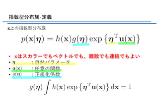
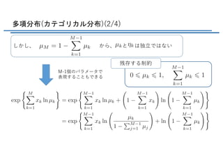
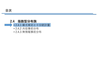
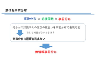
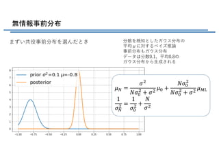
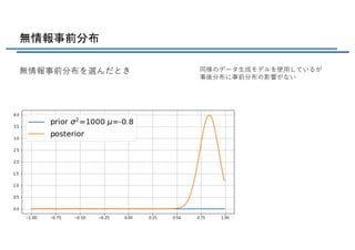
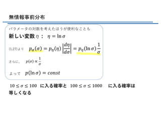
8. 多項分布(カテゴリカル分布)(3/4)
元の式に
代⼊しなおすと、
全てのkについて
⾜し合わせる
ソフトマックス関数
0
exp( )
( )
exp( )
k
k M
ii
x
f
x=
=
å
x
(右辺)
<latexit sha1_base64="THKcNOK4qWzxXlUiacxqMNDG3zE=">AAADE3ichVHLahRBFL3TiRrjIxPdCNkUDiMRYagWwSAIATeuQh5OEkiHobtTPVOZflFdPRqb/IB7cZFVAi4kn5BdFHTjThf5BHEZQRAXnq5pfMVHNV116tx77qOul4Yy05wf1ayR0VOnz4ydHT93/sLFifrkpeUsyZUv2n4SJmrVczMRyli0tdShWE2VcCMvFCte/15pXxkIlckkfqC3UrEeud1YBtJ3NahOPXainHVYwfpsm91lTqBcHzdHPEqZE4pATwNr97uLo2S3p68DFcxmN5iT5ZExbpbGP6k2f1Z16g3e4maxk8CuQIOqNZ/UX5NDG5SQTzlFJCgmDRySSxm+NbKJUwpunQpwCkgau6BtGoc2h5eAhwu2j72L21rFxriXMTOj9pElxK+gZNTk7/kLfszf8H3+gX/9a6zCxChr2cLpDbUi7Uw8ubL0+b+qCKem3g8VFM1/VK0poBlTrUT1qWHKPvxhhMHjZ8dLdxabxTW+xz+ig11+xF+ih3jwyX++IBZ3TEXKaAQ9ND1HpooYr1zAliHDBmwBuBzvoRG5QKYeDcoXxQDt38d1EizfbNm8ZS/caszOVaMcoym6StOY122apfs0T21kf0dfaiO1UeupdWAdWq+Grlat0lymX5b19huTYLv9</latexit>
<latexit sha1_base64="hAaEbLVE27hLYBsb50lDVyDUK0U=">AAADSnichVHNbtNAEB67BUoKNMAFicuKKFF6SLRGSKCiSJW4cADUH9JW6hbLcdeJ41+t1yll5RfgBThwAqkHxGNwgANXDn0ExI0iIQQHxhsDggrYlb2z38z3zczOIA39TFJ6aJgzsydOnpo7XZs/c/bcQv38hY0syYXL+24SJmJr4GQ89GPel74M+VYquBMNQr45CG6V/s0JF5mfxPflfsp3ImcY+57vOhIhu37QYmFMWMg92SbME45LFGFRTmw8A1LgVsQiHcKyPNLgGKEfAWMdwIQ/HMlF0iOMS+cnk7Fai7A7qKz9jhDJ3jSFQr4dFMrqlKq2Gves4oG627EK7RkXRY/xh6lql3p2sFjY9QbtUr3IccOqjAZUayWpvwYGu5CACzlEwCEGiXYIDmS4t8ECCiliO6AQE2j52s+hgBpyc4ziGOEgGuB/iLftCo3xXmpmmu1ilhA/gUwCTfqOvqBH9A19Sd/Tb3/VUlqjrGUfz8GUy1N74fGl9c//ZUV4Shj9YiGj+Y+qJXhwQ1frY/WpRso+3KnC5NGTo/WltaZq0ef0A3bwjB7SV9hDPPnkHqzytae6IqE5HPZ0z5GuIsZXVujLMMMu+jzEcnwPicoKM41gUr4oDtD6c1zHjY2rXYt2rdVrjeV71Sjn4DJcgTbO6zosw21YgT64xrxhGUvGTfOt+dH8Yn6dhppGxbkIv62Z2e+h4M/d</latexit>
<latexit sha1_base64="TSwki9nluWDHvkrir1/vyHRa8Js=">AAACyXichVE7axRRFP4yvmJ8ZBMbwSa4rthkuRMEJRAIpBFEycNNAtk4zEzuJpPMKzN31iSXqezyByysFCzExlZbC/0DFvkJYhnBxsJv7g6IBvUMc++53znfeXppGORKiKMh69TpM2fPDZ8fuXDx0uXRxtj4cp4UmS87fhIm2arn5jIMYtlRgQrlappJN/JCueLtzFX2lb7M8iCJH6n9VK5H7mYc9ALfVYScxo2Zbi9zfW2X2p7s5kXk6O0Zu3ysH0wS6kaFs12WTqMp2sLIxEnFrpUmaplPGh/RxQYS+CgQQSKGoh7CRc5vDTYEUmLr0MQyaoGxS5QYIbegl6SHS3SH5yZfazUa813FzA3bZ5aQf0bmBFris3gtjsUn8UZ8ET/+GkubGFUt+7y9AVemzujh1aXv/2VFvBW2frHIaP2jaoUe7ppqA1afGqTqwx9E6B88O16aXmzpm+Kl+MoOXogj8YE9xP1v/qsFufjcVJQZjsQT03Nkqog5ZU1bzgwbtPWIFZyHYmTNTFvoVxPlAu0/13VSWZ5q26JtL9xuzj6sVzmMa7iOW9zXHcziHubRYfZDvMU7vLfuW7vWnnUwcLWGas4V/CbW05/KsKXz</latexit>
<latexit sha1_base64="qzp3qU05umwGmLLs2hbezjCXyog=">AAAC13ichVFLS9xQFP6M2qq1dbQboRtxGBFKhxMRKsKA4Kabio+OWhwbknhHw+RFcjOiYeiuFHeuLHRVwYX0P3TThf4BF/6E4lLBjYue3AmKlbYn5N5zv3O+87RC14kl0XmH1tnV/ehxT2/fk/6nzwYKg0PLcZBEtqjagRtEq5YZC9fxRVU60hWrYSRMz3LFitWYzewrTRHFTuC/kzuhWPfMTd+pO7YpGTIKE5VanHhG2qjorQ/p21ZaE9I0Gq2K/vKe4ZV+azIKRSqTkpGHip4rReQyHxROUMMGAthI4EHAh2TdhYmYvzXoIISMrSNlLGLNUXaBFvqYm7CXYA+T0Qafm/xay1Gf31nMWLFtzuLyHzFzBCU6o2O6pFP6Tr/o5q+xUhUjq2WHb6vNFaExsDe8dP1flse3xNYdixmlf1QtUceUqtbh6kOFZH3Y7QjN3YPLpenFUjpGh3TBHXyjc/rJPfjNK/toQSx+VRVFiiOwrXr2VBU+TzllW8wZNthWZyzheUiOnHKmLTSzifIC9T/X9VBZnijrVNYXJoszc/kqe/ACoxjnfb3GDN5gHlXO/gU/cIJT7b32UfukfW67ah055znuibb/G87Qq9c=</latexit>
(左辺)

9. 多項分布(カテゴリカル分布)(4/4)
カテゴリカル分布はソフトマックス関数を⽤いた表現においても
によって対応付けられることから
指数型分布族の標準形になっている
<latexit sha1_base64="cHNej5Ktg6qD7gUwtThF+p3Jjmo=">AAADd3ichVFLa9RQFD6Z+Kj10aluBBdeHKZMkQ43UrAIQsGNG6WvaQtNOySZm0mYvEhuxo5x/oB/wIUrBRfiz3Cha8FFf4K4rCCCC7/ciYpt1RuS8+U75zuPe+wk8DPJ+YFW00+dPnN26tz0+QsXL83UZy9vZnGeOqLjxEGcbttWJgI/Eh3py0BsJ6mwQjsQW/bgXunfGoo08+NoQ44SsRta/ch3fceSoLr1DwlrMTO0pGe7rGD7bMyeMNOOg142CmHAmUJaoOfZXWYGwpUtZrCbzMzykHXhHoA34N8DfsAWFDbFfvIzWMkngXCkft+T879sKTpBclL9MlQ1moZAG2DGRxqvknbrDd7m6rDjwKhAg6qzEtffkUk9ismhnEISFJEEDsiiDM8OGcQpAbdLBbgUyFd+QWOahjZHlECEBXaAbx9/OxUb4b/MmSm1gyoB3hRKRk3+kb/mh/w9f8M/8e9/zVWoHGUvI1h7ohVJd+bp1fWv/1WFsJK83yoomv/oWpJLS6pbH90niinncCYZho+fHa7fWWsWc/wl/4wJXvAD/hYzRMMvzqtVsfZcdZQqjaBHauZQdRHhlgv4MlToweeCy3EfEpkLVPJoWN4oFmgcXddxsHmrbfC2sbrYWH5YrXKKrtENamFft2mZ7tMKdcjRlrQ9ra95tW/6dX1Ob01Ca1qluUJ/HN34AUy92YQ=</latexit>
<latexit sha1_base64="2l9vxtczbdtNcL2km7KN9s7Myxs=">AAADC3ichVE9axRBGH6z8SPGj5yxEWwGj5MIeswGQRGEgI2Nkq9LAtl47O7N3g2Z/WBn7uRc7g8I1hZWChZiaSd2IqZIa5GfIHZGsDCFz86tiAZ1jtt55nnmeT/mDTIlteF8b8KZPHL02PGpE9MnT50+M1M7O7um034eilaYqjTfCHwtlExEy0ijxEaWCz8OlFgPtm+X+vpA5FqmyaoZZmIr9ruJjGToG1DtWuQFqeroYYyNFcwTxmcjdot5SkRmbnxuQ3DBXgHbSY0uwU/+LrtaaZx5uez2zGV2vwwU+6aXx0CrUEftWp03uV3sMHArUKdqLaa1D+RRh1IKqU8xCUrIACvySeO3SS5xysBtUQEuB5JWFzSiaXj7uCVwwwe7jW8Xp82KTXAuY2rrDpFF4Z/DyajBP/KXfJ/v8Ff8Ez/4a6zCxihrGWIPxl6RtWcenV/59l9XjN1Q75cLjsY/qjYU0Q1brUT1mWXKPsJxhMHDJ/srN5cbxSX+nH9GB8/4Hn+HHpLB1/DFklh+aivKrUfQA9tzbKtI8MoFNI0MHWgRuD7ewyBygUw9GpQvigG6f47rMFibb7q86S5dqy/cq0Y5RRfoIs1hXtdpge7QIrWQfZe+0Hc6cB47r503ztvxVWei8pyj35bz/gc8qbpW</latexit>
<latexit sha1_base64="pYtNZg2paon8StH4xBwbnoJgSFY=">AAACr3ichVHLThRRED00KAOoDLoxcUOcjGE1qSYkEFYkblwRXsOQMIDdTQ1zQ7/SfWdg7PADfoAuXCgmLoif4UJ+wAWfYFxCwoYF1Xc6MULA6vS9dU/Vqacb+yrVRGcD1uDQg4fDpZHRsUePn4yXJ56up1En8bjuRX6UbLhOyr4Kua6V9nkjTtgJXJ8b7v7r3N7ocpKqKFzTvZi3AmcvVC3lOVqgZlPzoc4O2pzw0U65QjUyMnlbsQulgkKWovJPNLGLCB46CMAIoUX34SCVbxM2CLFgW8gES0RTxs44wqhwO+LF4uEIui/nnrw2CzSUdx4zNWxPsvjyJ8KcRJV+0Qmd0yl9p990dWeszMTIa+nJ7fa5HO+Mv3++evlfViC3RvsvSxjVe6rWaGHOVKuk+tggeR9eP0L33cfz1fmVavaKvtIf6eCYzuiH9BB2L7xvy7zyyVSUGA7jwPQcmCpCmXImtlQy7IqtJVhH5qElciaZ2ujmE5UF2jfXdVtZn67ZVLOXZyoLi8UqS3iBl5iSfc1iAW+whLpkj/EBn/HFsq2GtW297btaAwXnGf4RS10DCm2ccg==</latexit>
<latexit sha1_base64="xfnw6cCyV3er5ZC/e8yWGIYXLko=">AAADbnichVHLahRREK2e9hHHR0YFEUS8OEyYII63RVAEIeDGjZKHkwTSydDdc3u6mX7RfXvM2MwP+AMuXCm4ED/DhfoBLvIJ4kaI4MaFp++0CSY+7jBdVefUqVt1y04CP5Oc72g1/cjRY8dnTtRPnjp9ZrZx9txqFuepI7pOHMTpum1lIvAj0ZW+DMR6kgortAOxZg/vl/zaSKSZH0eP5TgRm6E1iHzXdywJqNf4aIaW9GyXFSxnE9Zm+/E24nk2d+8AZJp17895BjhWH5SkHQf9bBzCIMEU0tqrFQhXtpF6jZlZHrIe+CErtRO2Bf8hu658U2wnv5KVfpoIIvUHnpzfs6VISXqNJu9wddhhx6icJlVnMW68J5P6FJNDOYUkKCIJPyCLMvw2yCBOCbBNKoCl8HzFC5pQHdocWQIZFtAhvgNEGxUaIS5rZkrt4JYA/xRKRi3+ib/hu/wDf8s/8x9/rVWoGmUvY1h7qhVJb/bZxZXv/1WFsJK8fRUUrX90LcmlO6pbH90nCinncKYVRk+f767cXW4Vc/wV/4IJXvId/g4zRKNvzuslsfxCdZQqjaAnauZQdRHhlQtwGW7og3OB5XgPicoFbvJoVL4oFmgcXNdhZ/Vmx+AdY+lWc+FRtcoZukRXqY193aYFekCL1CVHu6F1tS2tV/uqX9Av61emqTWt0pyn347e/glcRtHm</latexit>

10. １変数ガウス分布(1/2)
𝑝 𝑥|𝜇, 𝜎( =
1
2𝜋𝜎( ⁄. (
exp −
1
2𝜎( 𝑥 − 𝜇 (
=
1
2𝜋𝜎( ⁄. (
exp −
1
2𝜎( 𝑥( +
𝜇
𝜎( 𝑥 −
1
2𝜎( 𝜇(
=
1
2𝜋𝜎( ⁄. (
exp −
1
2𝜎( 𝜇( exp −
1
2𝜎( 𝑥( +
𝜇
𝜎( 𝑥
=
1
2𝜋𝜎( ⁄. (
exp −
1
2𝜎( 𝜇( exp
⁄𝜇 𝜎(
− ⁄1 2𝜎(
4
𝑥
𝑥(

11. １変数ガウス分布(2/2)
つまり、１変数ガウス分布も以下の対応付けによって
指数型分布族であるといえる
𝜼 =
⁄𝜇 𝜎(
⁄−1 2𝜎(
𝐮 𝑥 =
𝑥
𝑥(
ℎ 𝑥 = 2𝜋 ⁄8. (
𝑔 𝜼 = −2𝜂(
⁄. ( 𝑒𝑥𝑝
𝜂.
(
4𝜂(

12. 目次
2.4 指数型分布族
• 2.4.1 最尤推定と⼗分統計量
• 2.4.2 共役事前分布
• 2.4.3 無情報事前分布

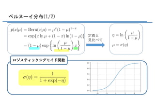
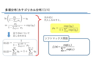
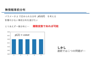
13. 最尤推定量と十分統計量(1/4)
パラメータベクトルηの推定をする
ηについて勾配をとる
{ } { }T T
( ) ( )exp ( ) ( ) ( )exp ( ) ( ) 0h d h dh h h hÑ + =ò òx u x x x u x u x xg g
{ }T
( ) ( )exp ( ) 1h dh h =ò x u x xg (2.195)
両辺を(2.195)で割る
{ } [ ]T( )
( ) ( )exp ( ) ( ) ( )
( )
h d
h
h h
h
Ñ
- = =ò x u x u x x Ε u x
g
g
g

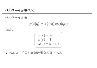
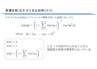
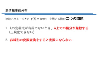
14. 最尤推定量と十分統計量 (2/4) 演習(2.58)
また、共分散については
より、⼆次微分から得られる
指数型分布族の分布を正規化できたなら、微分で簡単に分布の
モーメントがわかる
[ ] { }
{ } { }
[ ]
[ ]
T
T T T
T T
ln ( ) ( ) ( ) ( )exp ( ) ( )
ln ( ) ( ) ( )exp ( ) ( ) ( ) ( )exp ( ) ( ) ( )
( ) ( ) ( ) ( )
cov ( )
h d
h d h d
h h h
h h h h h
-Ñ = =
-ÑÑ = Ñ +
é ù é ù= - +ë û ë û
=
ò
ò ò
Ε u x x u x u x x
x u x u x x x u x u x u x x
Ε u x Ε u x Ε u x u x
u x
g g
g g g
[ ]ln ( ) ( )h-Ñ = Ε u xgつまり、 が得られる (2.226)

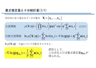
15. 最尤推定量と十分統計量(3/4)
同分布に従う独⽴なデータの集合 { }1, , N=X x x!
( ) T
11
| ( ) ( ) exp ( )
N N
N
n n
nn
p hh h h
==
æ ö ì ü
= í ýç ÷
î þè ø
åÕX x u xg尤度関数
対数尤度関数 ( ) T
1 1
ln | ln ( ) ln ( ) ( )
N N
n n
n n
p h Nh h h
= =
= + +å åX x u xg
( )ln |p hX のηについて勾配を０とすると、
原則として、
この式をとけば最尤推定量𝜼=>が
得られる。1
1
ln ( ) ( )
N
ML n
nN
h
=
-Ñ = åu xg
(2.227)

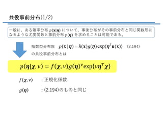
16. 最尤推定量と十分統計量(4/4)
1
1
ln ( ) ( )
N
ML n
nN
h
=
-Ñ = åu xg 最尤推定解は に依存する( )nnå u x
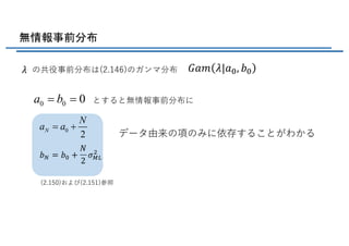
𝑁 → ∞の極限では…
上式の右辺は [ ]( )Ε u x になるため、(2.226)から最尤推定量が
真の値に等しくなることがわかる
ベイズ推論においてもこの⼗分性が成⽴する(８章にて)

17. 目次
2.4 指数型分布族
• 2.4.1 最尤推定と⼗分統計量
• 2.4.2 共役事前分布
• 2.4.3 無情報事前分布

18. 共役事前分布(1/2)
⼀般に、ある確率分布 𝑝(𝐱|𝜼) について、事後分布がその事前分布と同じ関数形に
なるような尤度関数と事前分布 𝑝(𝜼) を求めることは可能である。
指数型分布族
の共役事前分布とは
(2.194)
: 正規化係数
: (2.194)のものと同じ
𝑝 𝜼|𝝌, 𝜈 = 𝑓 𝝌, 𝜈 𝑔 𝜼 Gexp 𝜈𝜼H 𝝌
𝑓 𝝌, 𝜈
𝑔 𝜼

19. 共役事前分布(2/2)
尤度関数(2.227)と事前分布(2.229)の積を確認する
尤度関数
事前分布
事後分布をみると, 事前分布のパラメータνは
有効な事前の仮想観測値χの数だとみなせる
𝑝 𝜼|𝐗, 𝝌, 𝜈 ∝ 𝑔 𝜼 GKLexp 𝜼H M
NO.
L
𝐮 𝐱N + 𝜈𝝌

20. 目次
2.4 指数型分布族
• 2.4.1 最尤推定と⼗分統計量
• 2.4.2 共役事前分布
• 2.4.3 無情報事前分布

21. 無情報事前分布
事後分布 事前分布尤度関数∝ ×
何らかの知識やその信念の度合いを事前分布で表現可能
事前分布の影響を抑えたい
なにも知⾒がないときは？
無情報事前分布

22. 無情報事前分布
とりあえず⼀様分布に… 離散変数であれば可能
しかし
連続では⼆つの問題が…
パラメータ で定められる分布 を考える
影響の少ない事前分布を選びたい
𝜆 𝑝 𝑥|𝜆
𝑝 𝜆 = 𝑐𝑜𝑛𝑠𝑡

23. 無情報事前分布
連続パラメータλで を⽤いる際の⼆つの問題
1. λの定義域が有界でないとき、λ上での積分が発散する
(正規化できない)
2. ⾮線形の変数変換をすると定数にならない
𝑝 𝜆 = 𝑐𝑜𝑛𝑠𝑡

24. 無情報事前分布
変則事前分布 : 正規化できない分布
得られる事後分布が適切であれば(正規化できるのであれば)
使われることが多い

25. 無情報事前分布
変数変換にかかわる問題
関数:
問題なし
確率密度:
変数変換
定数じゃない
最尤推定ではこの問題は⽣じない
定数の事前分布を⽤いる際にはパラメータは
適切に表現できるよう注意して⽤いる必要がある
𝜆 = 𝜂(
ℎ 𝜆 = 𝑐𝑜𝑛𝑠𝑡
ℎ 𝜂( = 𝑐𝑜𝑛𝑠𝑡
𝑝V 𝜆 = 𝑐𝑜𝑛𝑠𝑡
𝑝V 𝜆 = 𝑝V 𝜆
𝑑𝜆
𝑑𝜂
= 𝑝V 𝜂( 2𝜂 ∝ 𝜂

26. 無情報事前分布
平⾏移動不変性
モデル(尤度関数) :
: 位置パラメータ
定数分だけ移動した においても、
ただし
新しい変数においても
確率密度は形状が同じ
𝑝 𝑥|𝜇 = 𝑓 𝑥 − 𝜇
𝜇
X𝑥 = 𝑥 + 𝑐
𝑝 X𝑥| ̂𝜇 = 𝑓 X𝑥 − ̂𝜇
X𝜇 ≡ 𝜇 + 𝑐

27. 無情報事前分布
事後分布 事前分布𝒑(𝝁)尤度関数𝒑 𝒙 𝝁∝ ×
平⾏移動不変性
事前分布にも平⾏移動不変性を
任意の定数cに対してμが区間 に⼊る確率と
区間 に⼊る確率が等しくなければならない
𝐴 ≤ 𝜇 ≤ 𝐵
𝐴 − 𝑐 ≤ 𝜇 ≤ 𝐵 − 𝑐

28. 無情報事前分布
任意のAとBについて上記が成⽴することから次が得られる
位置パラメータの例
ガウス分布の平均パラメータμなど
𝑝 𝜇 − 𝑐 = 𝑝 𝜇
⟺ 𝑝 𝜇 = 𝑐𝑜𝑛𝑠𝑡

29. 無情報事前分布
まずい共役事前分布を選んだとき 分散を既知としたガウス分布の
平均μに対するベイズ推論
事前分布もガウス分布
データは分散0.1、平均0.8の
ガウス分布から⽣成される
𝜇L =
𝜎(
𝑁𝜎b
( + 𝜎(
𝜇b +
𝑁𝜎b
(
𝑁𝜎b
( + 𝜎(
𝜇=>
1
𝜎L
( =
1
𝜎b
( +
𝑁
𝜎(

30. 無情報事前分布
無情報事前分布を選んだとき 同様のデータ⽣成モデルを使⽤しているが
事後分布に事前分布の影響がない

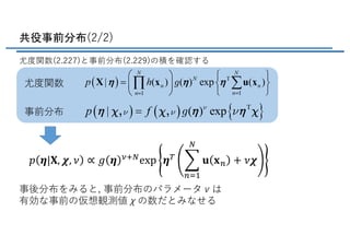
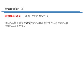
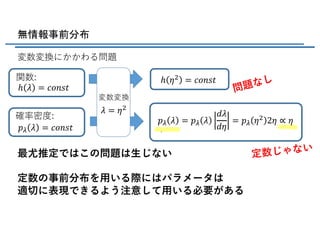
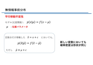
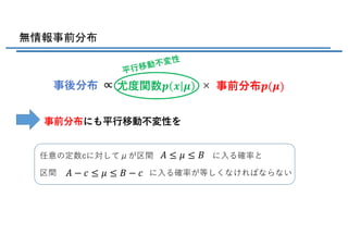
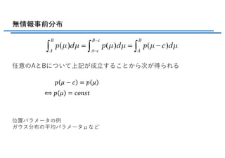
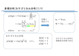
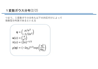
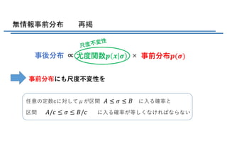
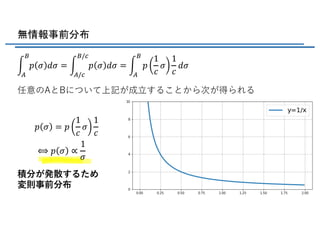
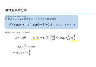
31. 無情報事前分布
尺度不変性
新しい変数においても
確率密度は形状が同じ定数倍だけ拡⼤縮⼩した においても、
ただし
モデル(尤度関数) :
: 尺度パラメータ
[m]から[km]への
尺度の変換などともとれる
𝑝 𝑥|𝜎 =
1
𝜎
𝑓
𝑥
𝜎
𝜎
X𝑥 = 𝑐𝑥
𝑝 X𝑥| X𝜎 =
1
X𝜎
𝑓
X𝑥
X𝜎
X𝜎 ≡ 𝑐𝜎

32. 無情報事前分布 再掲
事後分布 事前分布𝒑(𝝈)尤度関数𝒑 𝒙 𝝈∝ ×
尺度不変性
事前分布にも尺度不変性を
任意の定数cに対してμが区間 に⼊る確率と
区間 に⼊る確率が等しくなければならない
𝐴 ≤ 𝜎 ≤ 𝐵
𝐴/𝑐 ≤ 𝜎 ≤ 𝐵/𝑐

33. 無情報事前分布
任意のAとBについて上記が成⽴することから次が得られる
積分が発散するため
変則事前分布
e
f
g
𝑝 𝜎 𝑑𝜎 = e
f/h
g/h
𝑝 𝜎 𝑑𝜎 = e
f
g
𝑝
1
𝑐
𝜎
1
𝑐
𝑑𝜎
𝑝 𝜎 = 𝑝
1
𝑐
𝜎
1
𝑐
⟺ 𝑝 𝜎 ∝
1
𝜎

34. 無情報事前分布
に⼊る確率と に⼊る確率は
等しくなる
パラメータの対数を考えたほうが便利なことも
新しい変数η :
(1.27)より
さらに、
よって
𝜂 = ln 𝜎
𝑝k 𝜎 = 𝑝l 𝜂
𝑑𝜂
𝑑𝜎
= 𝑝l ln 𝜎
1
𝜎
𝑝 𝜎 ∝
1
𝜎
𝑝 ln 𝜎 = 𝑐𝑜𝑛𝑠𝑡
10 ≤ 𝜎 ≤ 100 100 ≤ 𝜎 ≤ 1000

35. 無情報事前分布
尺度パラメータの例 :
位置パラメータ考慮済みのガウス分布の標準偏差σ
ただし、
精度をつかうなら(1.27)から
𝒩 𝑥|𝜇, 𝜎( ∝ 𝜎8. 𝑒𝑥𝑝 − ⁄o𝑥 𝜎 ( o𝑥 = 𝑥 − 𝜇
𝜆 = ⁄1 𝜎( , 𝑝k 𝜎 = 𝑝V 𝜆
𝑑𝜆
𝑑𝜎
= −𝑝V 𝜆
3
𝜎q ∝
1
𝜎
−𝑝V 𝜆
3
𝜎( = 𝑐𝑜𝑛𝑠𝑡
⟺ 𝑝 𝜆 ∝ 𝜎( =
1
𝜆

36. 無情報事前分布
の共役事前分布は(2.146)のガンマ分布
0 0 0a b= = とすると無情報事前分布に
(2.150)および(2.151)参照
0
2
N
N
a a= +
データ由来の項のみに依存することがわかる
𝐺𝑎𝑚 𝜆|𝑎b, 𝑏b𝜆
𝑏L = 𝑏b +
𝑁
2
𝜎=>
(