The document presents an educational overview of elasticity in economics, primarily focusing on price elasticity of demand and supply, and how it relates to various factors like revenue, expenditure, and market conditions. It provides examples and scenarios to elucidate concepts like elastic and inelastic demand, calculating percentage changes, and the impact of substitutes on elasticity. Additionally, the document includes active learning exercises to reinforce comprehension of the subject matter.

1. InteractivePowerPoint Slides by:
V. Andreea Chiritescu
Eastern IllinoisUniversity
Elasticity and
Its Application
CHAPTER
5
N. GREGORY MANKIW
PRINCIPLES OF
ECONOMICS
NINTH EDITION
© 2021 Cengage Learning®. May not be scanned, copied or duplicated, or posted to a publicly accessible website, in whole or in part, except for use as permitted in a
license distributed with a certain product or service or otherwise on a password-protected website or school-approved learning management system for classroom use. 1
Modified by Joseph Tao-yi Wang

2. • What is elasticity?
• What kinds of issues can elasticity help us
understand?
• What is the price elasticity of demand?
How is it related to the demand curve?
How is it related to revenue and expenditure?
• What is the price elasticity of supply?
How is it related to the supply curve?
• What are the income and cross-price elasticities
of demand?
2
IN THIS CHAPTER
© 2021 Cengage Learning®. May not be scanned, copied or duplicated, or posted to a publicly accessible website, in whole or in part, except for use as permitted in a
license distributed with a certain product or service or otherwise on a password-protected website or school-approved learning management system for classroom use.

3. Our Scenario
3
• You maintain the social media accounts for local
businesses
– You charge NT$6,000 per business, and currently
maintain the social media accounts for 12
businesses per year.
• Your costs are rising (including the opportunity cost
of your time).
– You consider raising the price to NT$7,500.
• The law of demand: if you raise your price, you will
not have as many accounts to maintain.
– How many fewer accounts?
– How much will your revenue fall, or might it
increase?
© 2021 Cengage Learning®. May not be scanned, copied or duplicated, or posted to a publicly accessible website, in whole or in part, except for use as permitted in a
license distributed with a certain product or service or otherwise on a password-protected website or school-approved learning management system for classroom use.

4. The Elasticity of Demand
• Elasticity
– Measure of the responsiveness of Qd or Qs
to a change in one of its determinants
• Price elasticity of demand
– How much the quantity demanded of a
good responds to a change in the price of
that good
• Loosely speaking, it measures the price-
sensitivity of buyers’ demand
© 2021 Cengage Learning®. May not be scanned, copied or duplicated, or posted to a publicly accessible website, in whole or in part, except for use as permitted in a 4
license distributed with a certain product or service or otherwise on a password-protected website or school-approved learning management system for classroom use.

5. The Price Elasticity of Demand
5
Price elasticity of demand is
=
Along a D curve, P and Q
move in opposite directions,
which would make
price elasticity negative.
P
Q
D
P
P rises 2
by 10% P1
Q2 Q1
Q falls
by 15%
We will drop the minus sign and report all price elasticities as
positive numbers (absolute values).
© 2021 Cengage Learning®. May not be scanned, copied or duplicated, or posted to a publicly accessible website, in whole or in part, except for use as permitted in a
license distributed with a certain product or service or otherwise on a password-protected website or school-approved learning management system for classroom use.
15%
=
10%
= 1.5
Percentage change in Qd
Percentage change in P

6. Going from A to B:
• the % change in P = 25%
• the % change in Q = - 33%
Price elasticity = 33/25 = 1.33
We get different values!
Calculating Percentage Changes
6
Going from B to A:
• % change in P = - 20%
• % change in Q = 50%
Price elasticity =50/20 = 2.5
Q
D
B
P
$7500
$6000
8 12
A
Demand for maintaining
social media accounts
© 2021 Cengage Learning®. May not be scanned, copied or duplicated, or posted to a publicly accessible website, in whole or in part, except for use as permitted in a
license distributed with a certain product or service or otherwise on a password-protected website or school-approved learning management system for classroom use.
start value
Standard method of computing
the percentage (%) change:
end value – start value x 100%

7. The Price Elasticity of Demand
7
© 2021 Cengage Learning®. May not be scanned, copied or duplicated, or posted to a publicly accessible website, in whole or in part, except for use as permitted in a
license distributed with a certain product or service or otherwise on a password-protected website or school-approved learning management system for classroom use.
• Midpoint method
– The midpoint is the number halfway
between the start and end values
• The average of those values
• % change = end value – start value x 100%
midpoint
• Price elasticity of demand =

8. Our Scenario: Calculating Percentage Changes
Using the midpoint method
of computing % changes:
8
Q
D
B
P
$7500
$6000
8 12
A
Demand for maintaining
social media accounts
© 2021 Cengage Learning®. May not be scanned, copied or duplicated, or posted to a publicly accessible website, in whole or in part, except for use as permitted in a
license distributed with a certain product or service or otherwise on a password-protected website or school-approved learning management system for classroom use.
$7,500 – $6,000
$6,750
x 100%
= 22.2%
% change in P =
% change in Q =
12 – 8
x 100% = 40.0%
10
Price elasticity of demand = 40/22.2 = 1.8

9. Active Learning 1: Calculate an Elasticity
Use the following information to calculate the
price elasticity of demand for iPhone 12 Pro:
• if P = NT$35,900, Qd = 10,600
• if P = NT$52,400, Qd = 8,400
A. Use the midpoint method to calculate
percentage change in price
B. Use the midpoint method to calculate
percentage change in quantity
C. Calculate the price elasticity of demand
9
© 2021 Cengage Learning®. May not be scanned, copied or duplicated, or posted to a publicly accessible website, in whole or in part, except for use as permitted in a
license distributed with a certain product or service or otherwise on a password-protected website or school-approved learning management system for classroom use.

10. Active Learning 1: Answers
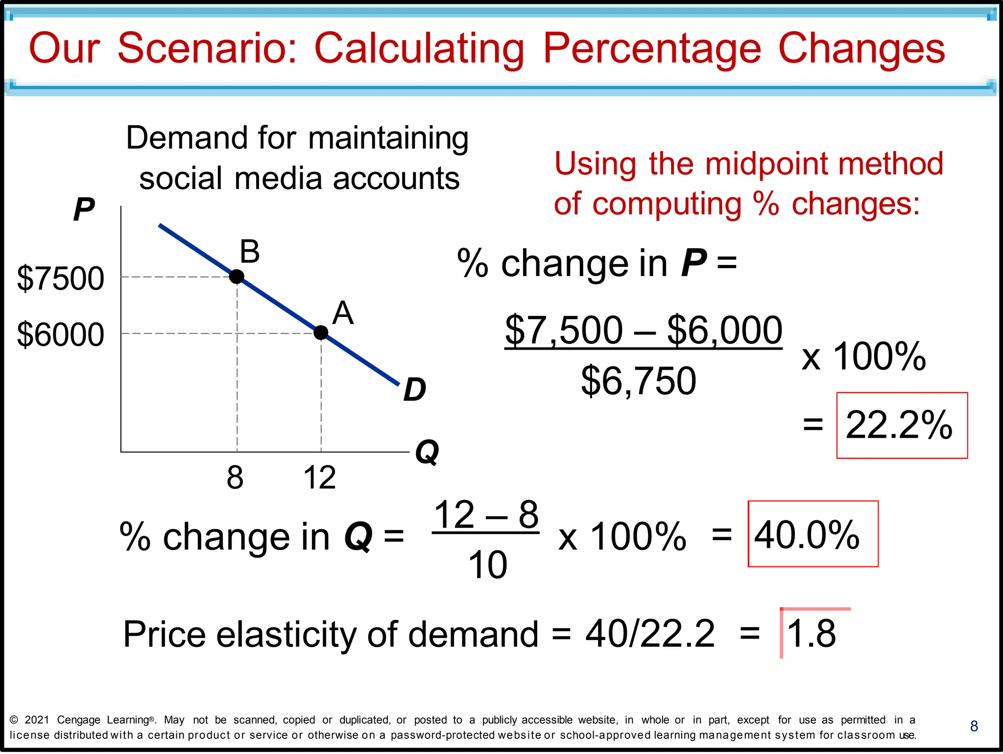
Using the midpoint method to calculate
percentage changes:
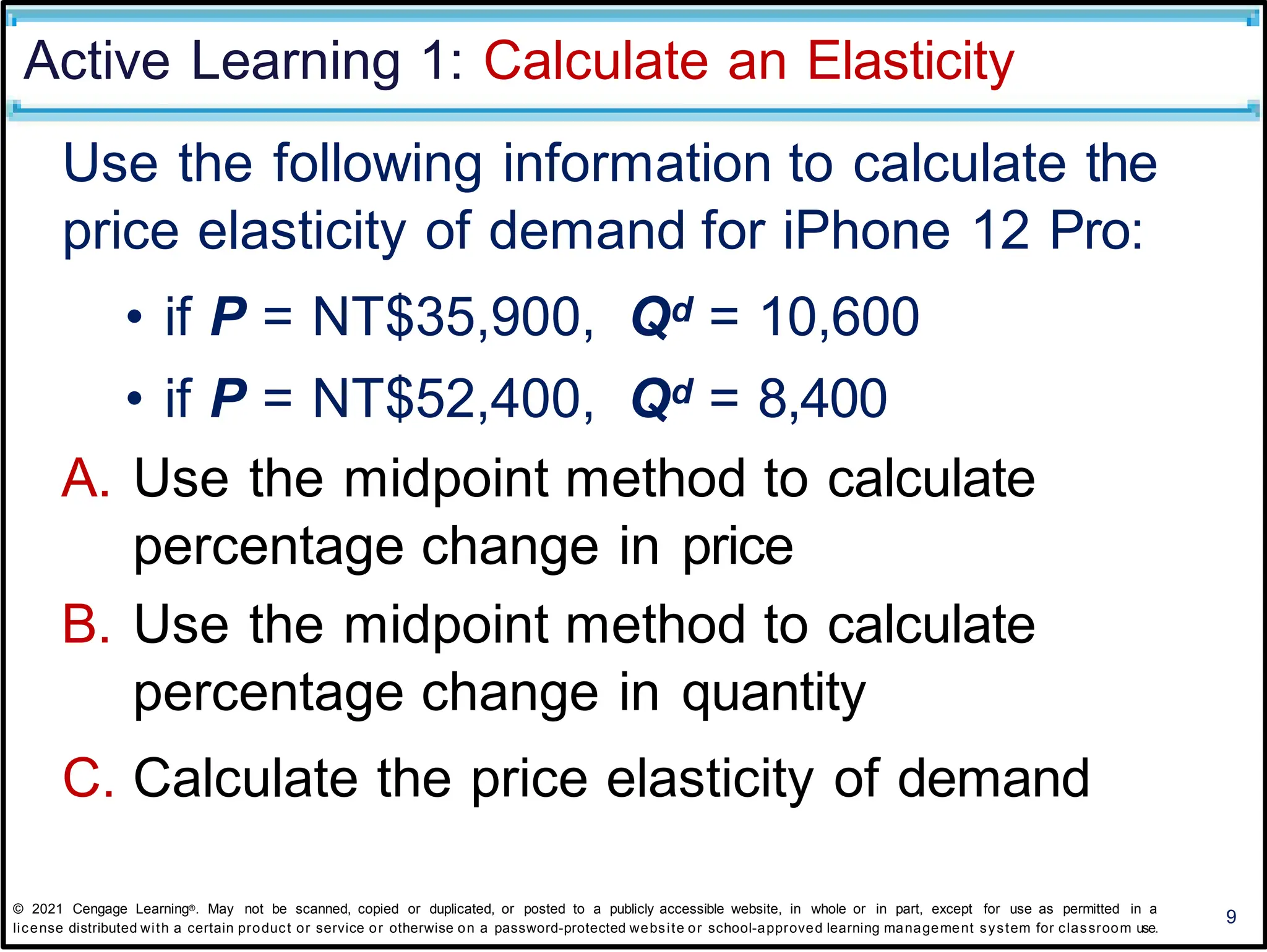
A. % change in P =
[($52,400 - $35,900)/$44,150] ×100 = 37.37%
B. % change in Qd =
[(10,600 – 8,400)/9,500] ×100 = 23.16%
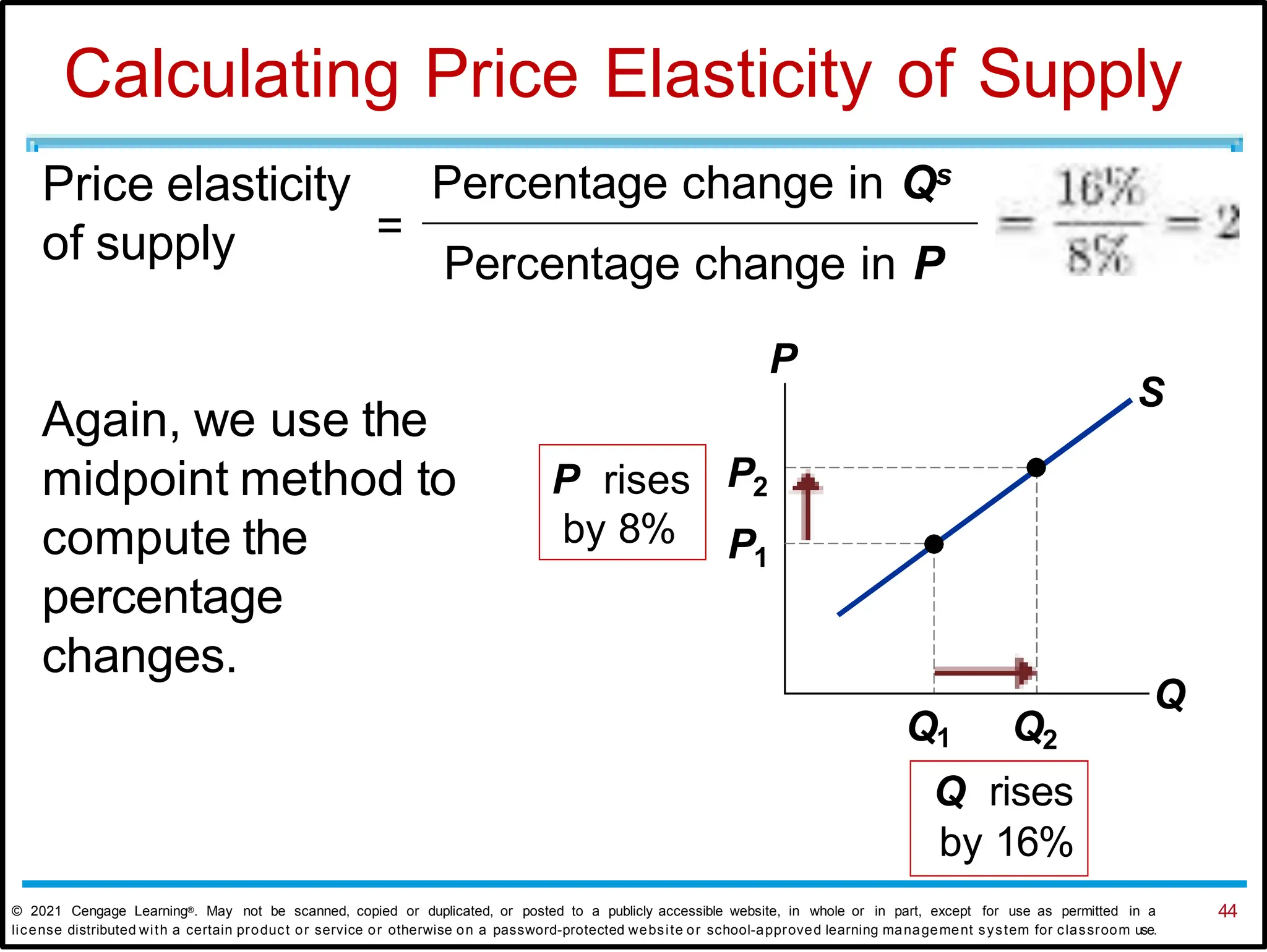
C. Price elasticity of demand =
= % change in Qd / % change in P
= 23.16/37.37 = 0.62
10
© 2021 Cengage Learning®. May not be scanned, copied or duplicated, or posted to a publicly accessible website, in whole or in part, except for use as permitted in a
license distributed with a certain product or service or otherwise on a password-protected website or school-approved learning management system for classroom use.

11. Determinants of Price Elasticity of Demand
We look at a series of examples comparing
two common goods.
• In each example:
– Suppose prices of both goods rise by 20%
– Which good has the highest price elasticity of
demand? Why?
– What lesson we learn about the determinants of
price elasticity of demand?
11
© 2021 Cengage Learning®. May not be scanned, copied or duplicated, or posted to a publicly accessible website, in whole or in part, except for use as permitted in a
license distributed with a certain product or service or otherwise on a password-protected website or school-approved learning management system for classroom use.

12. EXAMPLE 1: Samsung S20 vs. iPhone 12 Pro
12
• Prices of both of these goods rise by 20%.
For which good does Qd drop the most?
Why?
• Samsung S20 has many close substitutes, so
buyers can easily switch if the price rises
• iPhone 12 Pro has no close substitutes, so a
price increase would not affect demand much
Price elasticity is higher when close
substitutes are available.
© 2021 Cengage Learning®. May not be scanned, copied or duplicated, or posted to a publicly accessible website, in whole or in part, except for use as permitted in a
license distributed with a certain product or service or otherwise on a password-protected website or school-approved learning management system for classroom use.

13. EXAMPLE 2: Mountain Dew vs. Soda (Pop)
13
• Prices of both of these goods rise by 20%.
For which good does Qd drop the most?
Why?
• For a narrowly defined good, Mountain Dew,
there are many substitutes
• There are fewer substitutes available for
broadly defined goods (soda / pop)
Price elasticity is higher for narrowly defined
goods than for broadly defined ones.
© 2021 Cengage Learning®. May not be scanned, copied or duplicated, or posted to a publicly accessible website, in whole or in part, except for use as permitted in a
license distributed with a certain product or service or otherwise on a password-protected website or school-approved learning management system for classroom use.

14. EXAMPLE 3: Insulin vs. Rolex Watches
14
• Prices of both of these goods rise by 20%.
For which good does Qd drop the most?
Why?
• Insulin is a necessity to diabetics. A rise in
price would cause little or no decrease in
quantity demanded
• A Rolex watch is a luxury. If the price rises,
some people will forego it.
Price elasticity is higher for luxuries than for
necessities.
© 2021 Cengage Learning®. May not be scanned, copied or duplicated, or posted to a publicly accessible website, in whole or in part, except for use as permitted in a
license distributed with a certain product or service or otherwise on a password-protected website or school-approved learning management system for classroom use.

15. EXAMPLE 4: Gasoline, Short Run vs. Long Run
15
• The price of gasoline rises 20%. Does Qd
drop more in the short run or the long run?
Why?
• There’s not much people can do in the
short run, other than ride the bus or carpool.
• In the long run, people can buy smaller cars or
live closer to work.
Price elasticity is higher in the long run.
© 2021 Cengage Learning®. May not be scanned, copied or duplicated, or posted to a publicly accessible website, in whole or in part, except for use as permitted in a
license distributed with a certain product or service or otherwise on a password-protected website or school-approved learning management system for classroom use.

16. The Variety of Demand Curves – 1
• Demand is elastic
– Price elasticity of demand > 1
• Demand is inelastic
– Price elasticity of demand < 1
• Demand has unit elasticity
– Price elasticity of demand = 1
© 2021 Cengage Learning®. May not be scanned, copied or duplicated, or posted to a publicly accessible website, in whole or in part, except for use as permitted in a 16
license distributed with a certain product or service or otherwise on a password-protected website or school-approved learning management system for classroom use.

17. The Variety of Demand Curves – 2
• Demand is perfectly inelastic
– Price elasticity of demand = 0
– Demand curve is vertical
• Demand is perfectly elastic
– Price elasticity of demand = infinity
– Demand curve is horizontal
• The flatter the demand curve
– The greater the price elasticity of demand
17
© 2021 Cengage Learning®. May not be scanned, copied or duplicated, or posted to a publicly accessible website, in whole or in part, except for use as permitted in a
license distributed with a certain product or service or otherwise on a password-protected website or school-approved learning management system for classroom use.

18. Perfectly Inelastic Demand
18
• D curve:
Vertical
• Consumers’
price sensitivity:
None
• Elasticity:
0
0%
= 0
of demand % change in P 10%
Price elasticity =
% change in Q
=
Q1
D
P
Q
P1
P2
P falls
by 10%
Q changes
by 0%
© 2021 Cengage Learning®. May not be scanned, copied or duplicated, or posted to a publicly accessible website, in whole or in part, except for use as permitted in a
license distributed with a certain product or service or otherwise on a password-protected website or school-approved learning management system for classroom use.

19. Inelastic Demand
19
relatively steep
• Consumers’ price
sensitivity:
relatively low
• Elasticity:
<1
% change in P 10%
• D curve
Price elasticity
=
% change in Q
=
<10%
< 1
D
of demand
P
Q
P1
P2
Q1 Q2
Q rises less
than 10%
P falls
by 10%
© 2021 Cengage Learning®. May not be scanned, copied or duplicated, or posted to a publicly accessible website, in whole or in part, except for use as permitted in a
license distributed with a certain product or service or otherwise on a password-protected website or school-approved learning management system for classroom use.

20. Unit Elastic Demand
20
intermediate
slope
• Consumers’ price
sensitivity:
intermediate
• Elasticity:
=1
10%
= 1
of demand % change in P 10%
• D curve
Price elasticity
=
% change in Q
=
D
P
Q
P1
P2
Q1 Q2
Q rises
by 10%
P falls
by 10%
© 2021 Cengage Learning®. May not be scanned, copied or duplicated, or posted to a publicly accessible website, in whole or in part, except for use as permitted in a
license distributed with a certain product or service or otherwise on a password-protected website or school-approved learning management system for classroom use.

21. Elastic Demand
21
relatively flat
• Consumers’ price
sensitivity:
relatively high
• Elasticity:
>1
>10%
> 1
% change in P 10%
• D curve
Price elasticity
=
% change in Q
=
D
of demand
P
Q1 Q2 Q
P1
P2
Q rises more
than 10%
P falls
by 10%
© 2021 Cengage Learning®. May not be scanned, copied or duplicated, or posted to a publicly accessible website, in whole or in part, except for use as permitted in a
license distributed with a certain product or service or otherwise on a password-protected website or school-approved learning management system for classroom use.

22. Perfectly Elastic Demand
22
• D curve
horizontal
• Consumers’
price sensitivity:
extreme
= infinity
% change in P 0%
Price elasticity
=
% change in Q
=
any %
D
of demand
P
Q • Elasticity:
infinity
Q1 Q2
Q changes
by any %
P2 = P1
P changes
by 0%
© 2021 Cengage Learning®. May not be scanned, copied or duplicated, or posted to a publicly accessible website, in whole or in part, except for use as permitted in a
license distributed with a certain product or service or otherwise on a password-protected website or school-approved learning management system for classroom use.

23. A Few Elasticities From the Real World
23
© 2021 Cengage Learning®. May not be scanned, copied or duplicated, or posted to a publicly accessible website, in whole or in part, except for use as permitted in a
license distributed with a certain product or service or otherwise on a password-protected website or school-approved learning management system for classroom use.
Eggs 0.1
Healthcare 0.2
Cigarettes 0.4
Rice 0.5
Housing 0.7
Beef 1.6
Peanut Butter 1.7
Restaurant meals 2.3
Mountain Dew 4.4

24. Joseph Tao-yi Wang
Selected Price Elasticity (from Wiki)
⏵Rice[48]
⏵ -0.47 (Austria)
⏵ -0.80 (Bangladesh)
⏵ -0.80 (China)
⏵ -0.25 (Japan)
⏵ -0.55 (US)
2020/10/5 Elasticity
⏵Eggs
⏵-0.1 (US: HH only),[54]
⏵-0.35 (Canada),[55]
⏵-0.55 (South Africa)[56]
⏵Livestock
⏵-0.5 to -0.6
(Broiler Chickens)[44]

25. Joseph Tao-yi Wang
Selected Price Elasticity (from Wiki)
⏵Soft Drinks
⏵-0.8 to -1.0 (General)[51]
⏵-3.8 (Coca-Cola)[52]
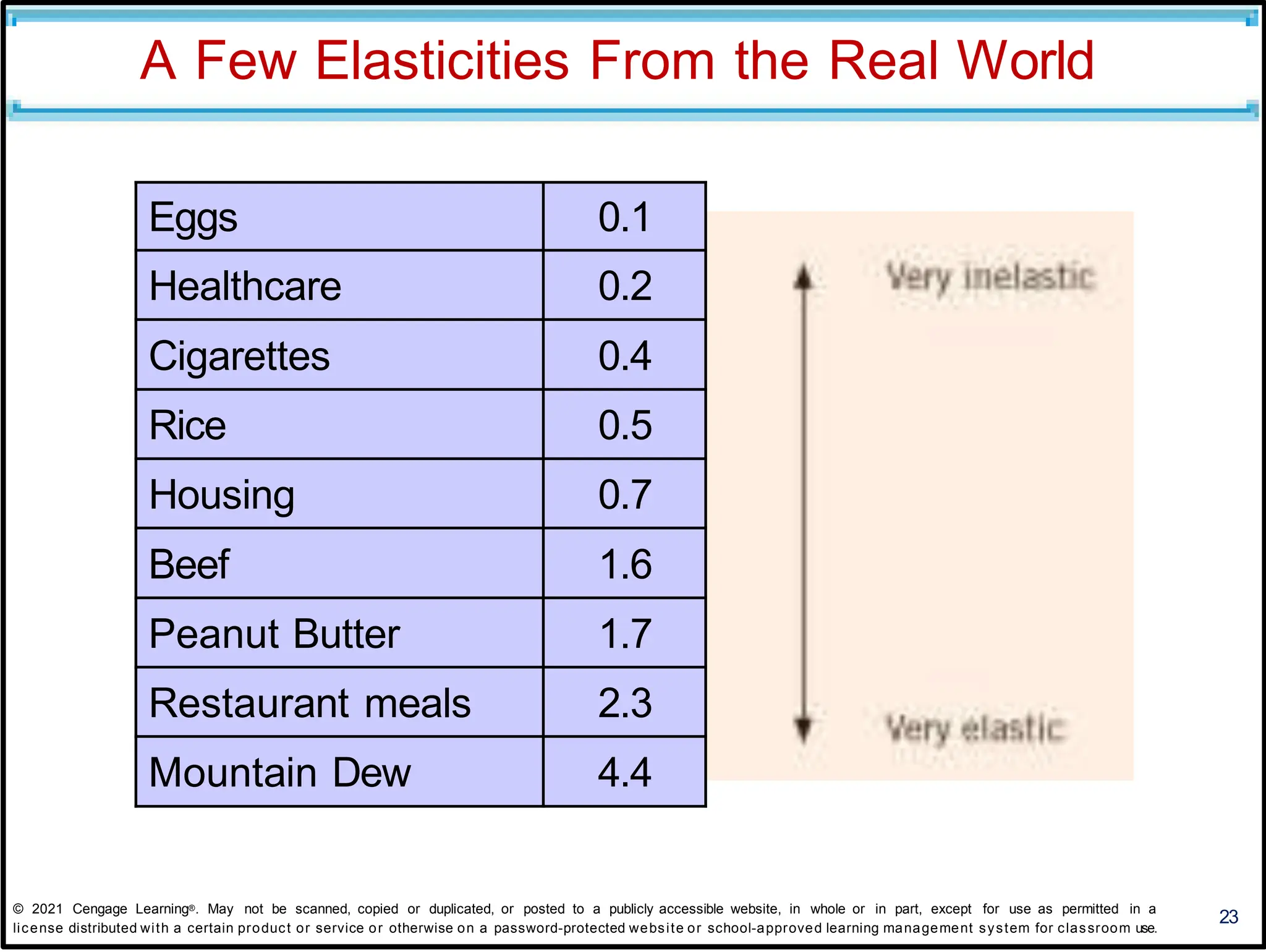
⏵-4.4 (Mountain Dew)[52]
⏵Cigarettes (US)[41]
⏵-0.3 to -0.6 (General)
⏵-0.6 to -0.7 (Youth)
2020/10/5 Elasticity
⏵Alcoholic
Beverages (US)[42]
⏵-0.3 or
-0.7 to -0.9
as of 1972 (Beer)
⏵-1.0 (Wine)
⏵-1.5 (Spirits)

26. Joseph Tao-yi Wang
Selected Price Elasticity (from Wiki)
⏵Transport
⏵-0.20 (Bus Travel US)[46]
⏵ -2.80 (Ford Compact
Automobile)[50]
2020/10/5 Elasticity
⏵Airline Travel (US)[43]
⏵-0.3 (First Class)
⏵-0.9 (Discount)
⏵-1.5 (Pleasure Travel)
⏵Car Fuel[45]
⏵-0.25 (Short Run)
⏵-0.64 (Long Run)

27. Joseph Tao-yi Wang
Selected Price Elasticity (from Wiki)
⏵Medicine (US)
⏵-0.31
(Medical Insurance)[46]
⏵-.03 to -.06
(Pediatric Visits) [47]
⏵Oil (World)
⏵-0.4
2020/10/5 Elasticity
⏵Cinema Visits (US)
⏵ -0.87 (General)[46]
⏵Live Performing Arts
(Theater, etc.)
⏵ -0.4 to -0.9 [49]
⏵Steel
⏵ -0.2 to -0.3[53]

28. Elasticity Along a Linear Demand Curve
28
The slope of a
linear demand
curve is constant,
but its elasticity
P
Q
$30
20
10
$0
0 20 40 60
40%
E =
200%
= 5.0
67%
E =
67%
= 1.0 is not.
200%
E =
40%
= 0.2
© 2021 Cengage Learning®. May not be scanned, copied or duplicated, or posted to a publicly accessible website, in whole or in part, except for use as permitted in a
license distributed with a certain product or service or otherwise on a password-protected website or school-approved learning management system for classroom use.

29. Our Scenario: Total Revenue
29
Continuing our scenario, if you raise your price
from $6,000 to $7,500, would your revenue
rise or fall?
Total Revenue (TR) = P x Q
• A price increase has two effects on revenue:
– Higher revenue: because of the higher P
– Lower revenue: you maintain fewer accounts
(lower Q)
• Which of these two effects is bigger?
– It depends on the price elasticity of demand
© 2021 Cengage Learning®. May not be scanned, copied or duplicated, or posted to a publicly accessible website, in whole or in part, except for use as permitted in a
license distributed with a certain product or service or otherwise on a password-protected website or school-approved learning management system for classroom use.

30. Our Scenario: Elastic Demand
30
Price elasticity of
demand = 1.8
• If P = NT$6,000,
Q = 12, and
TR = NT$72,000
• If P = NT$7,500,
Q = 8, and
TR = $60,000
When D is elastic,
a price increase causes
revenue to fall.
P
Q
D
lost revenue
due to lower Q
increased revenue
due to higher P
Demand for maintaining
social media accounts
$7500
$6000
8 12
© 2021 Cengage Learning®. May not be scanned, copied or duplicated, or posted to a publicly accessible website, in whole or in part, except for use as permitted in a
license distributed with a certain product or service or otherwise on a password-protected website or school-approved learning management system for classroom use.

31. Our Scenario: Inelastic Demand
31
Price elasticity of
demand = 0.82
• If P = NT$6,000,
Q = 12,
TR = NT$72,000
• If P = NT$7,500,
Q = 10, and
TR= NT$75,000
When D is inelastic,
a price increase causes
revenue to rise.
P
Q
D
lost revenue
due to lower Q
increased revenue
due to higher P
Demand for maintaining
social media accounts
12
$7500
$6000
10
© 2021 Cengage Learning®. May not be scanned, copied or duplicated, or posted to a publicly accessible website, in whole or in part, except for use as permitted in a
license distributed with a certain product or service or otherwise on a password-protected website or school-approved learning management system for classroom use.

32. Price Elasticity and Total Revenue
• For a price increase, if demand is elastic
 E > 1: % change in Q > % change in P
 TR decreases: the fall in revenue from lower
Q > the increase in revenue from higher P
• For a price increase, if demand is inelastic
 E < 1: % change in Q < % change in P
 TR increases: the fall in revenue from lower
Q < the increase in revenue from higher P
32
© 2021 Cengage Learning®. May not be scanned, copied or duplicated, or posted to a publicly accessible website, in whole or in part, except for use as permitted in a
license distributed with a certain product or service or otherwise on a password-protected website or school-approved learning management system for classroom use.

33. Active Learning 2: Elasticity and Total Revenue
A. Pharmacies raise the price of insulin by
10%.
– Does total expenditure on insulin rise or
fall?
B. As a result of a fare war, the price of a
luxury cruise falls 20%.
– Does luxury cruise companies’ total
revenue rise or fall?
33
© 2021 Cengage Learning®. May not be scanned, copied or duplicated, or posted to a publicly accessible website, in whole or in part, except for use as permitted in a
license distributed with a certain product or service or otherwise on a password-protected website or school-approved learning management system for classroom use.

34. Active Learning 2: Answers, A
34
A. Pharmacies raise the price of insulin by
10%.
– Does total expenditure on insulin rises or
falls?
• Expenditure = total revenue = P x Q
• Since demand for insulin is inelastic, Q will
fall less than 10%, so expenditure rises.
© 2021 Cengage Learning®. May not be scanned, copied or duplicated, or posted to a publicly accessible website, in whole or in part, except for use as permitted in a
license distributed with a certain product or service or otherwise on a password-protected website or school-approved learning management system for classroom use.

35. Active Learning 2: Answers, B
35
B. As a result of a fare war, the price of a
luxury cruise falls 20%.
– Does luxury cruise companies’ total
revenue rises or falls?
• Revenue = P x Q
• The fall in P reduces revenue, but Q increases,
which increases revenue. Which effect is
bigger?
• Since demand is elastic, Q will increase more
than 20%, so revenue rises.
© 2021 Cengage Learning®. May not be scanned, copied or duplicated, or posted to a publicly accessible website, in whole or in part, except for use as permitted in a
license distributed with a certain product or service or otherwise on a password-protected website or school-approved learning management system for classroom use.

36. Does Drug Interdiction Increase
or Decrease Drug-Related Crime?
1. Increase the number of federal agents
devoted to the war on drugs
– Illegal drugs: supply curve shifts left
2. Policy of drug education
– Reduce demand for illegal drugs
– Left shift of demand curve
36
© 2021 Cengage Learning®. May not be scanned, copied or duplicated, or posted to a publicly accessible website, in whole or in part, except for use as permitted in a
license distributed with a certain product or service or otherwise on a password-protected website or school-approved learning management system for classroom use.

37. Policy 1: Interdiction
37
Interdiction reduces
the supply of drugs.
• Demand for drugs
is inelastic: P rises
proportionally
more than Q falls.
Result: an increase
in total spending on
drugs, and in drug-
related crime.
Price of
Drugs
Quantity
of Drugs
S1
P1
P2
Q Q
2 1
new value of drug-
related crime
D1 S2
initial value
of drug-
related
crime
© 2021 Cengage Learning®. May not be scanned, copied or duplicated, or posted to a publicly accessible website, in whole or in part, except for use as permitted in a
license distributed with a certain product or service or otherwise on a password-protected website or school-approved learning management system for classroom use.

38. Does Drug Interdiction Increase
or Decrease Drug-Related Crime?
1. Increase the number of federal agents
devoted to the war on drugs
– Illegal drugs: supply curve shifts left
• Higher price and lower quantity
– Amount of drug-related crimes
• Inelastic demand for drugs
• Higher drugs price: higher total revenue
• Increase drug-related crime
38
© 2021 Cengage Learning®. May not be scanned, copied or duplicated, or posted to a publicly accessible website, in whole or in part, except for use as permitted in a
license distributed with a certain product or service or otherwise on a password-protected website or school-approved learning management system for classroom use.

39. Policy 2: Education
39
• P and Q fall.
Result:
A decrease in total
spending on drugs,
and in drug-related
crime.
Price of
Drugs
Education reduces
the demand for
drugs.
Quantity
of Drugs
S
P1
P2
Q2 Q1
initial value
of drug-
related
crime
new value of drug-
related crime
D2 D1
© 2021 Cengage Learning®. May not be scanned, copied or duplicated, or posted to a publicly accessible website, in whole or in part, except for use as permitted in a
license distributed with a certain product or service or otherwise on a password-protected website or school-approved learning management system for classroom use.

40. Does Drug Interdiction Increase
or Decrease Drug-Related Crime?
2. Policy of drug education
– Reduce demand for illegal drugs
– Left shift of demand curve
– Lower quantity
– Lower price
– Reduce drug-related crime
© 2021 Cengage Learning®. May not be scanned, copied or duplicated, or posted to a publicly accessible website, in whole or in part, except for use as permitted in a 40
license distributed with a certain product or service or otherwise on a password-protected website or school-approved learning management system for classroom use.

41. Income Elasticity of Demand
– How much the quantity demanded of a
good responds to a change in consumers’
income
– Percentage change in quantity demanded
– Divided by the percentage change in
income
• Normal goods: income elasticity > 0
• Inferior goods: income elasticity < 0
41
© 2021 Cengage Learning®. May not be scanned, copied or duplicated, or posted to a publicly accessible website, in whole or in part, except for use as permitted in a
license distributed with a certain product or service or otherwise on a password-protected website or school-approved learning management system for classroom use.

42. Cross-Price Elasticity of Demand
– How much the Qd of one good responds
to a change in the price of another good
– Percentage change in Qd of the first good
– Divided by the percentage change in price
of the second good
• Substitutes: cross-price elasticity > 0
• Complements: cross-price elasticity < 0
42
© 2021 Cengage Learning®. May not be scanned, copied or duplicated, or posted to a publicly accessible website, in whole or in part, except for use as permitted in a
license distributed with a certain product or service or otherwise on a password-protected website or school-approved learning management system for classroom use.

43. The Price Elasticity of Supply
– How much the quantity supplied of a good
responds to a change in the price of that
good
– Percentage change in quantity supplied
– Divided by the percentage change in price
• Loosely speaking, it measures sellers’
price-sensitivity
43
© 2021 Cengage Learning®. May not be scanned, copied or duplicated, or posted to a publicly accessible website, in whole or in part, except for use as permitted in a
license distributed with a certain product or service or otherwise on a password-protected website or school-approved learning management system for classroom use.

44. Calculating Price Elasticity of Supply
Again, we use the
midpoint method to
compute the
percentage
changes.
44
P
Q
S
Q1 Q2
P1
P rises P2
by 8%
Q rises
by 16%
© 2021 Cengage Learning®. May not be scanned, copied or duplicated, or posted to a publicly accessible website, in whole or in part, except for use as permitted in a
license distributed with a certain product or service or otherwise on a password-protected website or school-approved learning management system for classroom use.
=
Price elasticity Percentage change in Qs
of supply Percentage change in P

45. The Variety of Supply Curves – 1
• Supply is unit elastic
– Price elasticity of supply = 1
• Supply is elastic
– Price elasticity of supply > 1
• Supply is inelastic
– Price elasticity of supply < 1
© 2021 Cengage Learning®. May not be scanned, copied or duplicated, or posted to a publicly accessible website, in whole or in part, except for use as permitted in a 45
license distributed with a certain product or service or otherwise on a password-protected website or school-approved learning management system for classroom use.

46. The Variety of Supply Curves – 2
• Supply is perfectly inelastic
– Price elasticity of supply = 0
– Supply curve is vertical
• Supply is perfectly elastic
– Price elasticity of supply = infinity
– Supply curve is horizontal
• The flatter the supply curve
– The greater the price elasticity of supply
© 2021 Cengage Learning®. May not be scanned, copied or duplicated, or posted to a publicly accessible website, in whole or in part, except for use as permitted in a 46
license distributed with a certain product or service or otherwise on a password-protected website or school-approved learning management system for classroom use.

47. S
Perfectly Inelastic Supply
47
P
Q
Q1
Q changes
by 0%
0%
= 0
of supply
• S curve:
vertical
• Sellers’ price
sensitivity:
none
• Elasticity:
0
% change in P 10%
Price elasticity
=
% change in Q
=
P rises P2
by 10% P1
© 2021 Cengage Learning®. May not be scanned, copied or duplicated, or posted to a publicly accessible website, in whole or in part, except for use as permitted in a
license distributed with a certain product or service or otherwise on a password-protected website or school-approved learning management system for classroom use.

48. S
Inelastic Supply
• Sellers’ price
sensitivity:
relatively low
• Elasticity:
< 1
48
P
Q
Q Q
1 2
P2
P1
Q rises less
than 10%
of supply
• S curve:
relatively steep
% change in P 10%
Price elasticity
=
% change in Q
=
< 10%
< 1
P rises
by 10%
© 2021 Cengage Learning®. May not be scanned, copied or duplicated, or posted to a publicly accessible website, in whole or in part, except for use as permitted in a
license distributed with a certain product or service or otherwise on a password-protected website or school-approved learning management system for classroom use.

49. S
Unit Elastic Supply
intermediate
• Elasticity:
= 1
49
P
Q
Q Q
1 2
P2
P1
Q rises
by 10%
10%
10%
= 1
of supply
• S curve:
intermediate slope
• Sellers’ price
sensitivity:
% change in P
Price elasticity
=
% change in Q
=
P rises
by 10%
© 2021 Cengage Learning®. May not be scanned, copied or duplicated, or posted to a publicly accessible website, in whole or in part, except for use as permitted in a
license distributed with a certain product or service or otherwise on a password-protected website or school-approved learning management system for classroom use.

50. S
Elastic Supply
relatively high
• Elasticity:
> 1
50
P
Q
Q1 Q2
Q rises more
than 10%
> 10%
10%
> 1
of supply
• S curve:
relatively flat
• Sellers’ price
sensitivity:
% change in P
Price elasticity
=
% change in Q
=
P rises P2
by 10%
P 1
© 2021 Cengage Learning®. May not be scanned, copied or duplicated, or posted to a publicly accessible website, in whole or in part, except for use as permitted in a
license distributed with a certain product or service or otherwise on a password-protected website or school-approved learning management system for classroom use.

51. S
Perfectly Elastic Supply
51
P
Q
of supply
• S curve:
horizontal
• Sellers’ price
sensitivity:
extreme
• Elasticity:
infinity
% change in P 0%
Price elasticity
=
% change in Q
=
any %
= infinity
Q1 Q2
Q changes
by any %
P2 = P1
P changes
by 0%
© 2021 Cengage Learning®. May not be scanned, copied or duplicated, or posted to a publicly accessible website, in whole or in part, except for use as permitted in a
license distributed with a certain product or service or otherwise on a password-protected website or school-approved learning management system for classroom use.

52. The Determinants of Supply Elasticity
• Greater price elasticity of supply
– The more easily sellers can change the
quantity they produce
• Price elasticity of supply is greater in the
long run than in the short run
– In the long run: firms can build new factories,
or new firms may be able to enter the market
© 2021 Cengage Learning®. May not be scanned, copied or duplicated, or posted to a publicly accessible website, in whole or in part, except for use as permitted in a 52
license distributed with a certain product or service or otherwise on a password-protected website or school-approved learning management system for classroom use.

53. Active Learning 3: Elasticity and Changes in Equilibrium
Assume the supply of residential apartments is
inelastic and the supply of pork is elastic.
Suppose population growth causes demand for
both goods to double (at each price, Qd doubles).
• For which product will P change the most?
• For which product will Q change the most?
A. Draw a graph with the new equilibrium in the
market for housing
B. Draw a graph with the new equilibrium in the
market for pork
53
© 2021 Cengage Learning®. May not be scanned, copied or duplicated, or posted to a publicly accessible website, in whole or in part, except for use as permitted in a
license distributed with a certain product or service or otherwise on a password-protected website or school-approved learning management system for classroom use.

54. Active Learning 3A. Residential Apartments
54
When supply is
inelastic, an
increase in
demand has a
bigger impact on
price than on
quantity.
Residential Apartments
(inelastic supply):
S
P
Q
P1
A
D1 D2
B
Q1 Q2
P2
© 2021 Cengage Learning®. May not be scanned, copied or duplicated, or posted to a publicly accessible website, in whole or in part, except for use as permitted in a
license distributed with a certain product or service or otherwise on a password-protected website or school-approved learning management system for classroom use.

55. S
Active Learning 3B. Pork
55
When supply
is elastic,
an increase in
demand has a
bigger impact on
quantity than on
price.
Pork
(elastic supply):
P
Q
A
D1 D2
Q1 Q2
P2
P1
B
© 2021 Cengage Learning®. May not be scanned, copied or duplicated, or posted to a publicly accessible website, in whole or in part, except for use as permitted in a
license distributed with a certain product or service or otherwise on a password-protected website or school-approved learning management system for classroom use.

56. How the Price Elasticity of Supply Can Vary
56
• Supply often becomes less elastic as Q rises, due
to capacity limits.
Price
$15
Supply
500 525 Quantity
4
3
0 100 200
Elasticity is small
(less than 1).
12
Elasticity is large
(greater than 1).
© 2021 Cengage Learning®. May not be scanned, copied or duplicated, or posted to a publicly accessible website, in whole or in part, except for use as permitted in a
license distributed with a certain product or service or otherwise on a password-protected website or school-approved learning management system for classroom use.

57. More Applications – 1
1. Can Good News for Farming Be Bad
News for Farmers?
– New hybrid of wheat: 20% increased
production per acre
• Supply curve shifts to the right
• Higher quantity and lower price
• Demand is inelastic: total revenue falls
• Total profit falls if per acre cost is the same
– Paradox of public policy: induce farmers
not to plant crops
© 2021 Cengage Learning®. May not be scanned, copied or duplicated, or posted to a publicly accessible website, in whole or in part, except for use as permitted in a 57
license distributed with a certain product or service or otherwise on a password-protected website or school-approved learning management system for classroom use.

58. An increase in supply in the market for wheat
58
S2
Price of
Wheat
Quantity of Wheat
0
2
100 110
1. When demand is inelastic,
an increase in supply . . .
S1
2. … leads
$3
to a large
fall in
price. . .
3. … and a proportionately
smaller increase in quantity
sold. As a result, revenue
falls from $300 to $220.
Demand
© 2021 Cengage Learning®. May not be scanned, copied or duplicated, or posted to a publicly accessible website, in whole or in part, except for use as permitted in a
license distributed with a certain product or service or otherwise on a password-protected website or school-approved learning management system for classroom use.

59. More Applications – 2
2. Why Did OPEC Fail to Keep the Price of
Oil High?
– Increase in prices 1973-1974, 1971-1981
– Short-run: supply and demand are
inelastic
• Decrease in supply: large increase in price
– Long-run: supply and demand are elastic
• Decrease in supply: small increase in price
59
© 2021 Cengage Learning®. May not be scanned, copied or duplicated, or posted to a publicly accessible website, in whole or in part, except for use as permitted in a
license distributed with a certain product or service or otherwise on a password-protected website or school-approved learning management system for classroom use.

60. A Reduction in Supply in the World Market for Oil
60
Price
Price
P2
Demand
(a) The Oil Market in the Short Run (b) The Oil Market in the Long Run
S1
S2
P1
1. In the short run, when supply and
demand are inelastic, a shift in
supply. . .
1
S2 S
P2
P1
1. In the long run, when
supply and demand are
elastic, a shift in supply. . .
2. … leads to a
small increase
in price
Demand
Quantity
2. … leads to a
large increase in
price
0 Quantity
0
© 2021 Cengage Learning®. May not be scanned, copied or duplicated, or posted to a publicly accessible website, in whole or in part, except for use as permitted in a
license distributed with a certain product or service or otherwise on a password-protected website or school-approved learning management system for classroom use.

61. THINK-PAIR-SHARE
In order to reduce teen smoking, the
government places NT$20 per pack tax on cigarettes.
After one month, the quantity demanded of cigarettes
has been reduced only slightly. Discuss the following:
A. What conclusion can you draw about the one-
month demand for cigarettes?
B. Caleb suggests that the cigarette industry should
get together and raise the price of cigarettes
further to increase total revenue.
C. Keisha suggests that only your firm should raise
the price of your cigarettes to increase total
revenue.
61
© 2021 Cengage Learning®. May not be scanned, copied or duplicated, or posted to a publicly accessible website, in whole or in part, except for use as permitted in a
license distributed with a certain product or service or otherwise on a password-protected website or school-approved learning management system for classroom use.

62. • The price elasticity of demand
– Measures how much the quantity demanded
responds to changes in the price.
– Is the percentage change in quantity demanded
divided by the percentage change in price.
– If < 1, inelastic demand: quantity demanded
moves proportionately less than the price
– If > 1, elastic demand: quantity demanded
moves proportionately more than the price
62
CHAPTER IN A NUTSHELL
© 2021 Cengage Learning®. May not be scanned, copied or duplicated, or posted to a publicly accessible website, in whole or in part, except for use as permitted in a
license distributed with a certain product or service or otherwise on a password-protected website or school-approved learning management system for classroom use.

63. • Demand tends to be more elastic if
– Close substitutes are available
– The good is a luxury rather than a necessity
– The market is narrowly defined
– If buyers have substantial time to react to a price
change.
• Total revenue (PxQ), total amount paid for a good
– Moves in the same direction as P (inelastic D)
– Moves in the opposite direction as P (elastic D)
63
CHAPTER IN A NUTSHELL
© 2021 Cengage Learning®. May not be scanned, copied or duplicated, or posted to a publicly accessible website, in whole or in part, except for use as permitted in a
license distributed with a certain product or service or otherwise on a password-protected website or school-approved learning management system for classroom use.

64. • The income elasticity of demand
– Measures how much the quantity demanded
responds to changes in consumers’ income
• The cross-price elasticity of demand
– Measures how much the quantity demanded of
one good responds to changes in the price of
another good
• The tools of supply and demand can be applied to
many different kinds of markets. This chapter uses
them to analyze the market for wheat, the market
for oil, and the market for illegal drugs.
64
CHAPTER IN A NUTSHELL
© 2021 Cengage Learning®. May not be scanned, copied or duplicated, or posted to a publicly accessible website, in whole or in part, except for use as permitted in a
license distributed with a certain product or service or otherwise on a password-protected website or school-approved learning management system for classroom use.

65. • The price elasticity of supply
– Measures how much the quantity supplied responds
to changes in the price.
– Is the percentage change in quantity supplied
divided by the percentage change in price
– If < 1, inelastic supply: quantity supplied moves
proportionately less than the price
– If > 1, elastic supply: quantity supplied moves
proportionately more than the price
– Depends on the time horizon under consideration.
In most markets, supply is more elastic in the long
run than in the short run.
65
CHAPTER IN A NUTSHELL
© 2021 Cengage Learning®. May not be scanned, copied or duplicated, or posted to a publicly accessible website, in whole or in part, except for use as permitted in a
license distributed with a certain product or service or otherwise on a password-protected website or school-approved learning management system for classroom use.

66. Chapter 5: Elasticity
⏵Different Types of Elasticities
⏵Price Elasticity
⏵Income Elasticity
⏵Cross Price Elasticity
⏵Homework:
⏵Mankiw, Ch. 5, Problem 2, 7-12
⏵Challenge Questions/ex-Midterm
⏵2007 - Q2
⏵2008 - Part D ( + Multi-Choice Q4-Q5)
2020/10/5 Elasticity Joseph Tao-yi Wang

67. Chapter 5: Challenge Questions/ex-Midterm
⏵2009 - Part C5-C8 ( + Multiple Choice Q10)
⏵2010 - (True/False Q4)
⏵2012 - Part C ( + True/False Q5-6)
⏵2013 - Part A3-A4, B ( + True/False Q4-5)
⏵2014 - Part C1
⏵2015 - Part B1-B3 ( + True/False A6)
⏵2016 - Part A, B3-B4, F
⏵2017 - Part B (except possibly B3)
⏵2018 - Part A2-A4
⏵2019 - Part A4-A10, C1-C4
2020/10/5 Elasticity Joseph Tao-yi Wang