Ch 21 the theory of consumer choice

1. © 2009 South-Western, a part of Cengage Learning, all rights reserved
C H A P T E R
The Theory of
Consumer Choice
Microeonomics
P R I N C I P L E S O F
N. Gregory Mankiw
Premium PowerPoint Slides
by Ron Cronovich
21

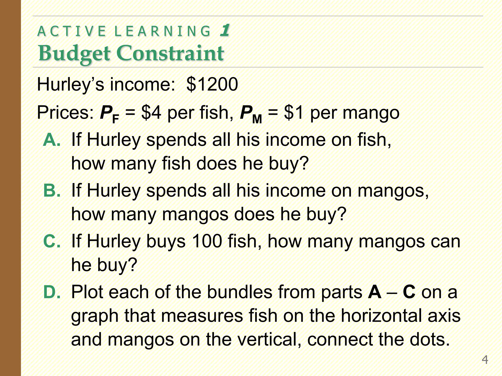
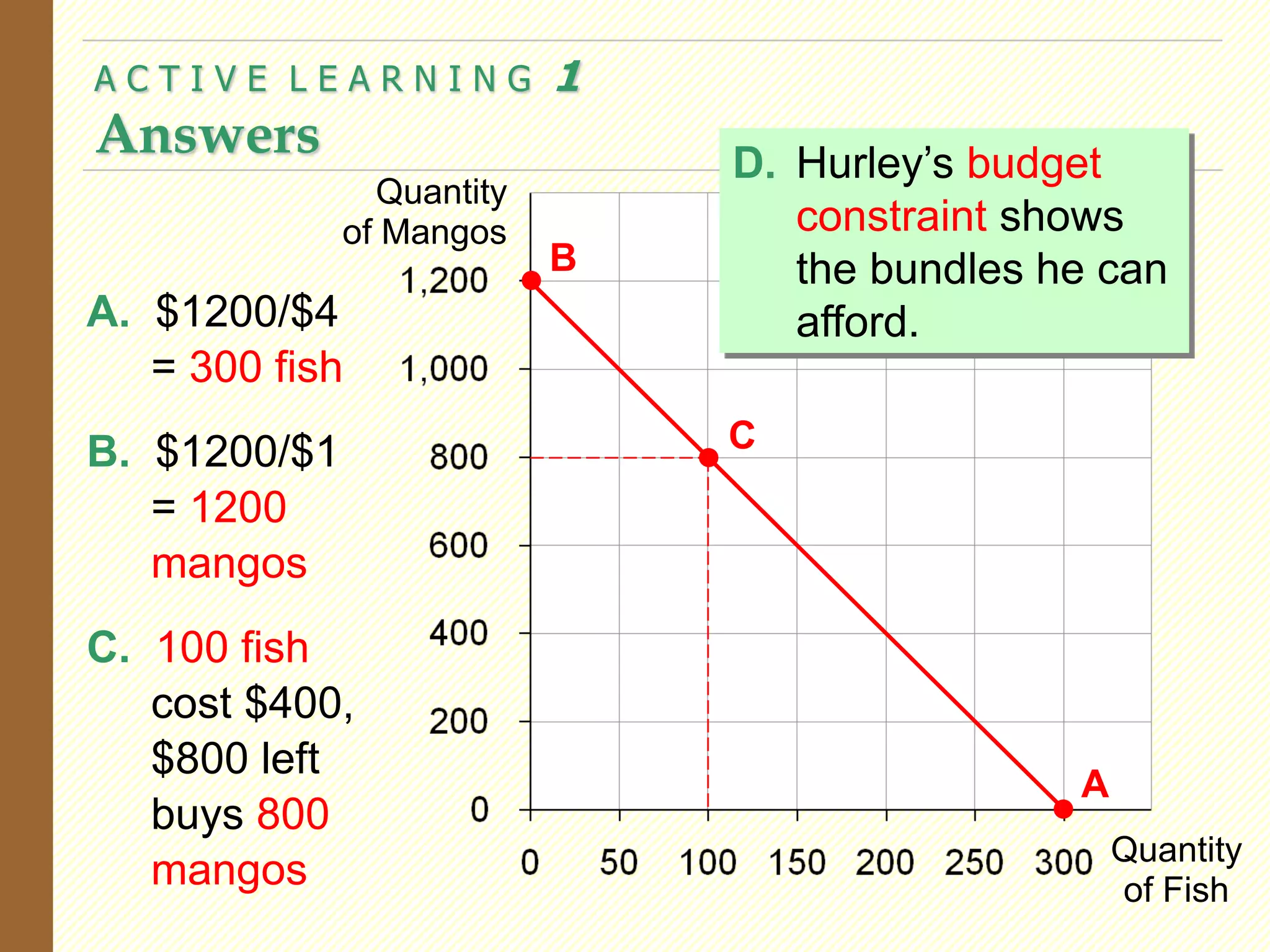
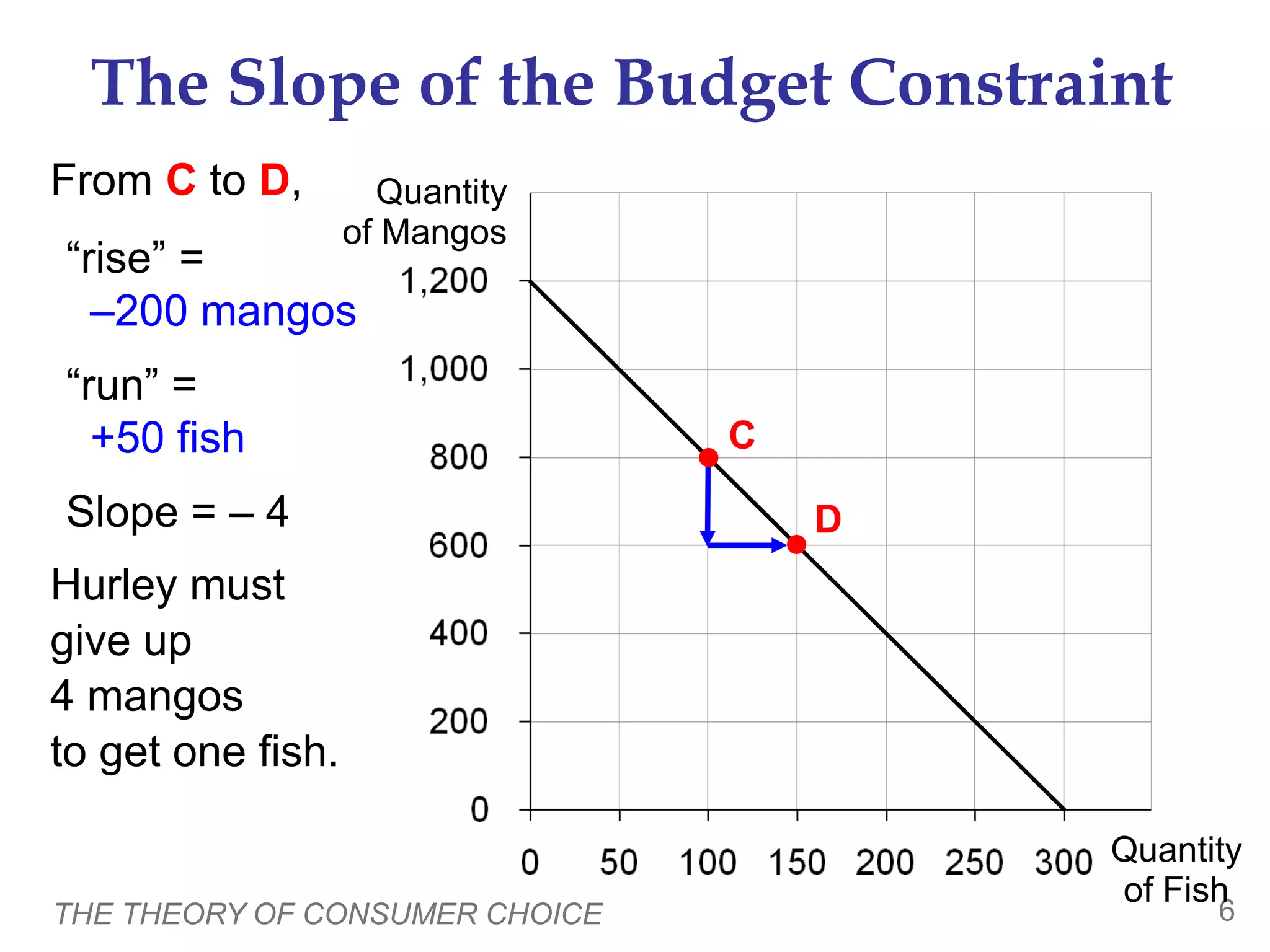
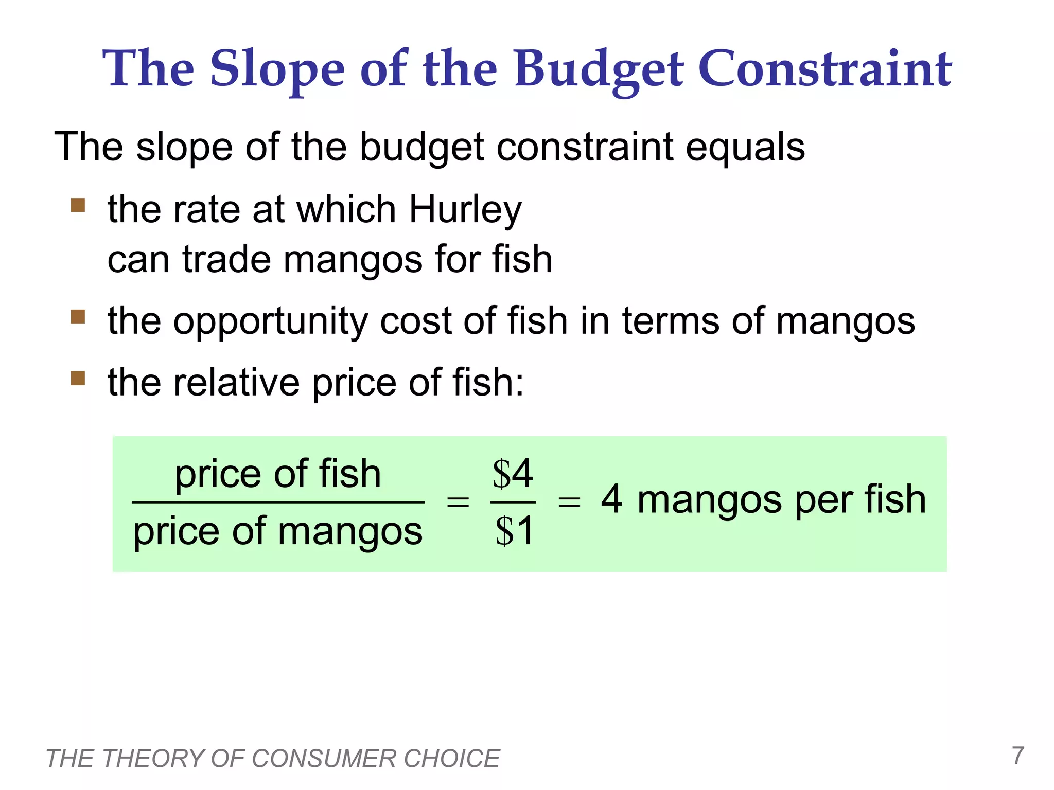
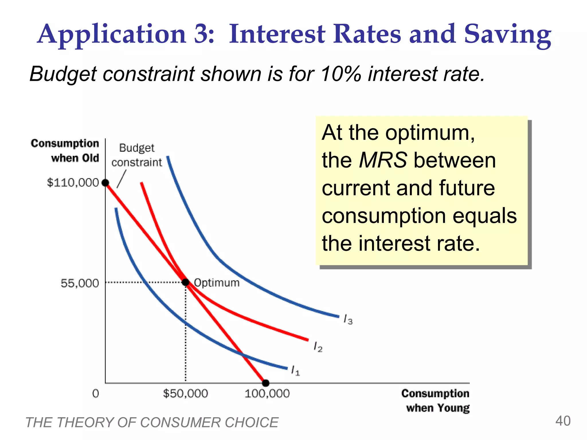
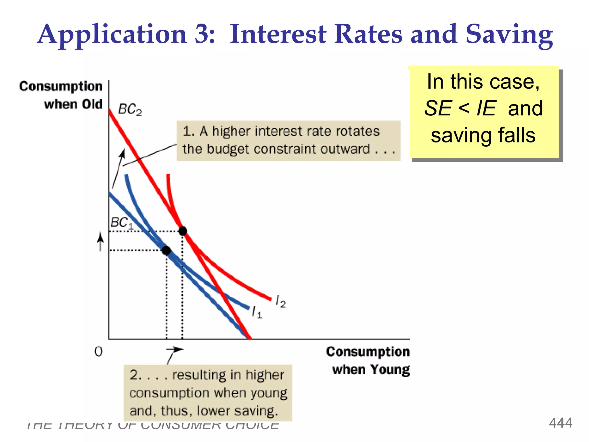
2. In this chapter,
look for the answers to these questions:
 How does the budget constraint represent the
choices a consumer can afford?
 How do indifference curves represent the
consumer’s preferences?
 What determines how a consumer divides her
resources between two goods?
 How does the theory of consumer choice explain
decisions such as how much a consumer saves,
or how much labor she supplies?
1

3. THE THEORY OF CONSUMER CHOICE 2
Introduction
 Recall one of the Ten Principles from Chapter 1:
People face tradeoffs.
 Buying more of one good leaves
less income to buy other goods.
 Working more hours means more income and
more consumption, but less leisure time.
 Reducing saving allows more consumption today
but reduces future consumption.
 This chapter explores how consumers make
choices like these.

4. THE THEORY OF CONSUMER CHOICE 3
The Budget Constraint:
What the Consumer Can Afford
 Example:
Hurley divides his income between two goods:
fish and mangos.
 A “consumption bundle” is a particular combination
of the goods, e.g., 40 fish & 300 mangos.
 Budget constraint: the limit on the consumption
bundles that a consumer can afford

5. Hurley’s income: $1200
Prices: PF = $4 per fish, PM = $1 per mango
A. If Hurley spends all his income on fish,
how many fish does he buy?
B. If Hurley spends all his income on mangos,
how many mangos does he buy?
C. If Hurley buys 100 fish, how many mangos can
he buy?
D. Plot each of the bundles from parts A – C on a
graph that measures fish on the horizontal axis
and mangos on the vertical, connect the dots.
A C T I V E L E A R N I N G 1
Budget Constraint
4

6. A. $1200/$4
= 300 fish
B. $1200/$1
= 1200
mangos
C. 100 fish
cost $400,
$800 left
buys 800
mangos
A C T I V E L E A R N I N G 1
Answers
Quantity
of Fish
Quantity
of Mangos
A
B
C
D. Hurley’s budget
constraint shows
the bundles he can
afford.

7. THE THEORY OF CONSUMER CHOICE 6
The Slope of the Budget Constraint
Quantity
of Fish
Quantity
of Mangos
D
From C to D,
“rise” =
–200 mangos
“run” =
+50 fish
Slope = – 4
Hurley must
give up
4 mangos
to get one fish.
C

8. THE THEORY OF CONSUMER CHOICE 7
The Slope of the Budget Constraint
The slope of the budget constraint equals
 the rate at which Hurley
can trade mangos for fish
 the opportunity cost of fish in terms of mangos
 the relative price of fish:
$
$
 
price of fish 4
4 mangos per fish
price of mangos 1

9. Show what happens to Hurley’s budget constraint if:
A. His income falls to $800.
B. The price of mangos rises to
PM = $2 per mango
A C T I V E L E A R N I N G 2
Budget constraint, continued.
8

10. Now,
Hurley
can buy
$800/$4
= 200 fish
or
$800/$1
= 800 mangos
or any
combination in
between.
A C T I V E L E A R N I N G 2
Answers, part A
Quantity
of Fish
Quantity
of Mangos
A fall in income
shifts the budget
constraint down.

11. Hurley
can still buy
300 fish.
But now he
can only buy
$1200/$2 =
600 mangos.
Notice:
slope is smaller,
relative price of
fish is now only
2 mangos.
A C T I V E L E A R N I N G 2
Answers, part B
Quantity
of Fish
Quantity
of Mangos
An increase in the
price of one good
pivots the budget
constraint inward.

12. THE THEORY OF CONSUMER CHOICE 11
Preferences: What the Consumer Wants
Quantity
of Fish
Quantity
of Mangos
Indifference curve:
shows consumption
bundles that give the
consumer the same
level of satisfaction
A, B, and all other
bundles on I1 make
Hurley equally happy –
he is indifferent
between them.
I1
One of Hurley’s
indifference curves
B
A

13. THE THEORY OF CONSUMER CHOICE 12
Four Properties of Indifference Curves
Quantity
of Fish
Quantity
of Mangos
If the quantity of
fish is reduced,
the quantity of
mangos must be
increased to keep
Hurley equally
happy.
A
One of Hurley’s
indifference curves
I1
1. Indifference curves
are downward-
sloping.
B

14. THE THEORY OF CONSUMER CHOICE 13
Four Properties of Indifference Curves
Quantity
of Fish
Quantity
of Mangos
Hurley prefers every
bundle on I2 (like C)
to every bundle on I1
(like A).
A few of Hurley’s
indifference curves
I1
I2
I0
D
2. Higher indifference
curves are preferred
to lower ones.
He prefers every
bundle on I1 (like A)
to every bundle on I0
(like D).
C
A

15. THE THEORY OF CONSUMER CHOICE 14
Four Properties of Indifference Curves
Quantity
of Fish
Quantity
of Mangos
Suppose they did.
Hurley should prefer
B to C, since B has
more of both goods.
Yet, Hurley is indifferent
between B and C:
He likes C as much as A
(both are on I4).
He likes A as much as B
(both are on I1).
Hurley’s
indifference curves
I1
3. Indifference curves
cannot cross.
B
C
I4
A

16. THE THEORY OF CONSUMER CHOICE 15
Four Properties of Indifference Curves
Quantity
of Fish
Quantity
of Mangos
Hurley is willing to give
up more mangos for a
fish if he has few fish
(A) than if he has
many (B).
4. Indifference curves
are bowed inward.
I1
1
1
6
2
A
B

17. THE THEORY OF CONSUMER CHOICE 16
The Marginal Rate of Substitution
Quantity
of Fish
Quantity
of Mangos
Hurley’s MRS is the
amount of mangos he
would substitute for
another fish. I1
1
1
6
2
A
B
Marginal rate of
substitution (MRS):
the rate at which a consumer
is willing to trade one good for
another.
MRS = slope of
indifference curve
MRS =
MRS =
MRS falls as you move
down along an
indifference curve.

18. THE THEORY OF CONSUMER CHOICE 17
One Extreme Case: Perfect Substitutes
Perfect substitutes: two goods with
straight-line indifference curves,
constant MRS
Example: nickels & dimes
Consumer is always willing to trade
two nickels for one dime.

19. THE THEORY OF CONSUMER CHOICE 18
Another Extreme Case: Perfect Complements
Perfect complements: two goods with
right-angle indifference curves
Example: Left shoes, right shoes
{7 left shoes, 5 right shoes}
is just as good as
{5 left shoes, 5 right shoes}

20. Less Extreme Cases:
Close Substitutes and Close Complements
Quantity
of Coke
Quantity
of Pepsi
Indifference
curves for close
substitutes are
not very bowed
Quantity
of hot dogs
Quantity
of hot
dog buns
Indifference
curves for
close
complements
are very
bowed

21. THE THEORY OF CONSUMER CHOICE 20
Optimization: What the Consumer Chooses
Quantity
of Fish
Quantity
of Mangos
1200
600
300
150
A is the optimum:
the point on the
budget constraint
that touches the
highest possible
indifference curve.
Hurley prefers B to A,
but he cannot afford B. A
C
D
Hurley can afford C
and D,
but A is on a higher
indifference curve.
B
The optimum
is the bundle
Hurley most
prefers out of
all the bundles
he can afford.

22. THE THEORY OF CONSUMER CHOICE 21
Optimization: What the Consumer Chooses
Quantity
of Fish
Quantity
of Mangos
1200
600
300
150
At the optimum,
slope of the
indifference curve
equals
slope of the budget
constraint:
MRS = PF/PM A
marginal
value of fish
(in terms of
mangos)
price of fish
(in terms of
mangos)
Consumer
optimization is
another example
of “thinking at the
margin.”

23. THE THEORY OF CONSUMER CHOICE 22
The Effects of an Increase in Income
Quantity
of Fish
Quantity
of Mangos
An increase in
income shifts the
budget constraint
outward.
If both goods are
“normal,” Hurley
buys more of each.
A
B

24.  An increase in income increases the quantity
demanded of normal goods and reduces the
quantity demanded of inferior goods.
 Suppose fish is a normal good
but mangos are an inferior good.
 Use a diagram to show the effects of
an increase in income on Hurley’s optimal
bundle of fish and mangos.
A C T I V E L E A R N I N G 3
Inferior vs. normal goods
23

25. A C T I V E L E A R N I N G 3
Answers
24
Quantity
of Fish
Quantity
of Mangos
If mangos are
inferior, the new
optimum will
contain fewer
mangos.
A
B

26. THE THEORY OF CONSUMER CHOICE 25
500
350
The Effects of a Price Change
Quantity
of Fish
Quantity
of Mangos
1200
600
300
150 600
initial
optimum
new
optimum
Initially,
PF = $4
PM = $1
PF falls to $2
budget constraint
rotates outward,
Hurley buys
more fish and
fewer mangos.

27. THE THEORY OF CONSUMER CHOICE 26
A fall in the price of fish has two effects on
Hurley’s optimal consumption of both goods.
 Income effect
A fall in PF boosts the purchasing power of Hurley’s
income, allows him to buy more mangos and more
fish.
 Substitution effect
A fall in PF makes mangos more expensive relative
to fish, causes Hurley to buy fewer mangos & more
fish.
Notice: The net effect on mangos is ambiguous.
The Income and Substitution Effects

28. THE THEORY OF CONSUMER CHOICE 27
The Income and Substitution Effects
Initial
optimum at A.
PF falls.
Substitution effect:
from A to B,
buy more fish and
fewer mangos.
Income effect:
from B to C,
buy more of both
goods.
Quantity
of Fish
Quantity
of Mangos
A
B
C
In this example,
the net effect
on mangos is
negative.

29. Do you think the substitution effect would be
bigger for substitutes or complements?
 Draw an indifference curve for Coke and Pepsi,
and, on a separate graph, one for hot dogs and
hot dog buns.
 On each graph, show the effects of a relative
price change (keeping the consumer on the initial
indifference curve).
A C T I V E L E A R N I N G 4
The substitution effect in two cases
28

30. But the substitution effect is bigger for substitutes
than complements.
A C T I V E L E A R N I N G 4
Answers
Quantity
of Coke
Quantity
of Pepsi
In both graphs, the relative price changes
by the same amount.
Quantity
of hot dogs
Quantity of
hot dog buns
A
B
A
B

31. $2
DFish
Deriving Hurley’s Demand Curve for Fish
350 Quantity
of Fish
Quantity
of Mangos
Quantity
of Fish
Price of
Fish
150
A
B
150
$4
A
350
B
30
A: When PF = $4, Hurley demands 150 fish.
B: When PF = $2, Hurley demands 350 fish.

32. THE THEORY OF CONSUMER CHOICE 31
Application 1: Giffen Goods
 Do all goods obey the Law of Demand?
 Suppose the goods are potatoes and meat,
and potatoes are an inferior good.
 If price of potatoes rises,
 substitution effect: buy less potatoes
 income effect: buy more potatoes
 If income effect > substitution effect,
then potatoes are a Giffen good, a good for which
an increase in price raises the quantity demanded.

33. THE THEORY OF CONSUMER CHOICE 32
Application 1:
Giffen Goods

34. THE THEORY OF CONSUMER CHOICE 33
Application 2: Wages and Labor Supply
Budget constraint
 Shows a person’s tradeoff between consumption
and leisure.
 Depends on how much time she has to divide
between leisure and working.
 The relative price of an hour of leisure is the amount
of consumption she could buy with an hour’s wages.
Indifference curve
 Shows “bundles” of consumption and leisure
that give her the same level of satisfaction.

35. THE THEORY OF CONSUMER CHOICE 34
Application 2: Wages and Labor Supply
At the optimum,
the MRS between
leisure and
consumption
equals the wage.

36. THE THEORY OF CONSUMER CHOICE 35
Application 2: Wages and Labor Supply
An increase in the wage has two effects
on the optimal quantity of labor supplied.
 Substitution effect (SE): A higher wage makes
leisure more expensive relative to consumption.
The person chooses less leisure,
i.e., increases quantity of labor supplied.
 Income effect (IE): With a higher wage,
she can afford more of both “goods.”
She chooses more leisure,
i.e., reduces quantity of labor supplied.

37. THE THEORY OF CONSUMER CHOICE 36
Application 2: Wages and Labor Supply
For this person,
SE > IE
So her labor supply
increases with the wage

38. THE THEORY OF CONSUMER CHOICE 37
Application 2: Wages and Labor Supply
For this person,
SE < IE
So his labor supply falls
when the wage rises

39. THE THEORY OF CONSUMER CHOICE 38
Could This Happen in the Real World???
Cases where the income effect on labor supply is
very strong:
 Over last 100 years, technological progress has
increased labor demand and real wages.
The average workweek fell from 6 to 5 days.
 When a person wins the lottery or receives an
inheritance, his wage is unchanged – hence no
substitution effect.
But such persons are more likely to work fewer
hours, indicating a strong income effect.

40. THE THEORY OF CONSUMER CHOICE 39
Application 3: Interest Rates and Saving
 A person lives for two periods.
 Period 1: young, works, earns $100,000
consumption = $100,000 minus amount saved
 Period 2: old, retired
consumption = saving from Period 1
plus interest earned on saving
 The interest rate determines
the relative price of consumption when young
in terms of consumption when old.

41. THE THEORY OF CONSUMER CHOICE 40
Application 3: Interest Rates and Saving
At the optimum,
the MRS between
current and future
consumption equals
the interest rate.
Budget constraint shown is for 10% interest rate.

42.  Suppose the interest rate rises.
 Describe the income and substitution effects on
current and future consumption, and on saving.
A C T I V E L E A R N I N G 5
Effects of a change in the interest rate
41

43. The interest rate rises.
Substitution effect
 Current consumption becomes more expensive
relative to future consumption.
 Current consumption falls, saving rises,
future consumption rises.
Income effect
 Can afford more consumption in both the
present and the future. Saving falls.
A C T I V E L E A R N I N G 5
Answers
42

44. THE THEORY OF CONSUMER CHOICE 43
Application 3: Interest Rates and Saving
In this case,
SE > IE and
saving rises

45. THE THEORY OF CONSUMER CHOICE 44
Application 3: Interest Rates and Saving
In this case,
SE < IE and
saving falls
44

46. THE THEORY OF CONSUMER CHOICE 45
CONCLUSION:
Do People Really Think This Way?
 People do not make spending decisions
by writing down their budget constraints and
indifference curves.
 Yet, they try to make the choices that maximize
their satisfaction given their limited resources.
 The theory in this chapter is only intended as a
metaphor for how consumers make decisions.
 It explains consumer behavior fairly well in many
situations and provides the basis for more
advanced economic analysis.

47. CHAPTER SUMMARY
 A consumer’s budget constraint shows the
possible combinations of different goods she can
buy given her income and the prices of the goods.
The slope of the budget constraint equals the
relative price of the goods.
 An increase in income shifts the budget constraint
outward. A change in the price of one of the goods
pivots the budget constraint.
46

48. CHAPTER SUMMARY
 A consumer’s indifference curves represent her
preferences. An indifference curve shows all the
bundles that give the consumer a certain level of
happiness. The consumer prefers points on higher
indifference curves to points on lower ones.
 The slope of an indifference curve at any point is
the marginal rate of substitution – the rate at which
the consumer is willing to trade one good for the
other.
47

49. CHAPTER SUMMARY
 The consumer optimizes by choosing the point on
her budget constraint that lies on the highest
indifference curve. At this point, the marginal rate
of substitution equals the relative price of the two
goods.
 When the price of a good falls, the impact on the
consumer’s choices can be broken down into two
effects, an income effect and a substitution effect.
48

50. CHAPTER SUMMARY
 The income effect is the change in consumption
that arises because a lower price makes the
consumer better off. It is represented by a
movement from a lower indifference curve to a
higher one.
 The substitution effect is the change that arises
because a price change encourages greater
consumption of the good that has become
relatively cheaper. It is represented by a
movement along an indifference curve.
49

51. CHAPTER SUMMARY
 The theory of consumer choice can be applied in
many situations. It can explain why demand
curves can potentially slope upward, why higher
wages could either increase or decrease labor
supply, and why higher interest rates could either
increase or decrease saving.
50