Download to read offline
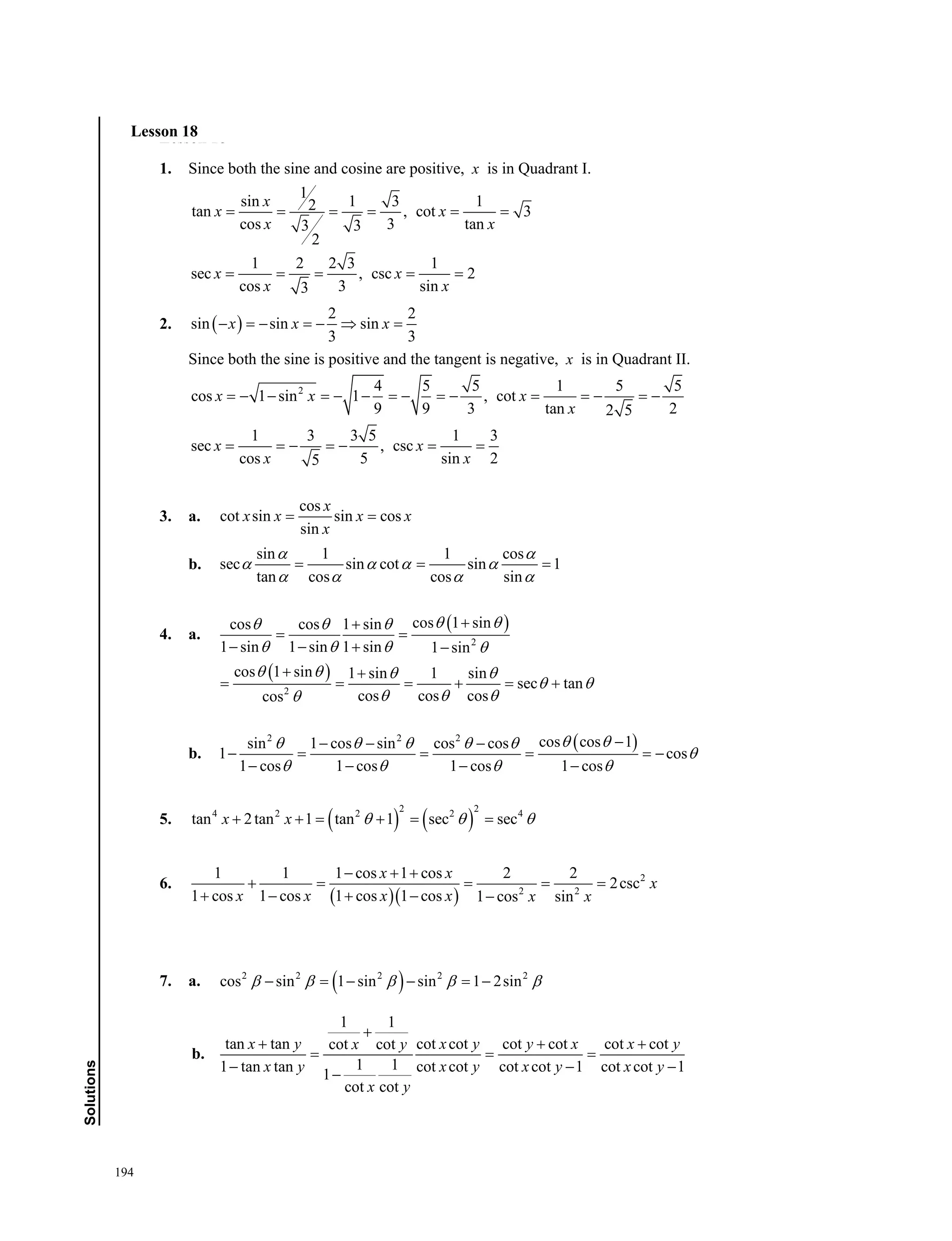
![THE GREAT COURSES®
Corporate Headquarters
4840 Westfields Boulevard, Suite 500
Chantilly, VA 20151-2299
USA
Phone: 1-800-832-2412
www.thegreatcourses.com
Course No. 1005 © 2011 The Teaching Company.
Cover Image: © Marek Uliasz/iStockphoto.
PB1005A
“Pure intellectual stimulation that can be popped
into the [audio or video player] anytime.”
—Harvard Magazine
“Passionate, erudite, living legend lecturers. Academia’s
best lecturers are being captured on tape.”
—The Los Angeles Times
“A serious force in American education.”
—The Wall Street Journal
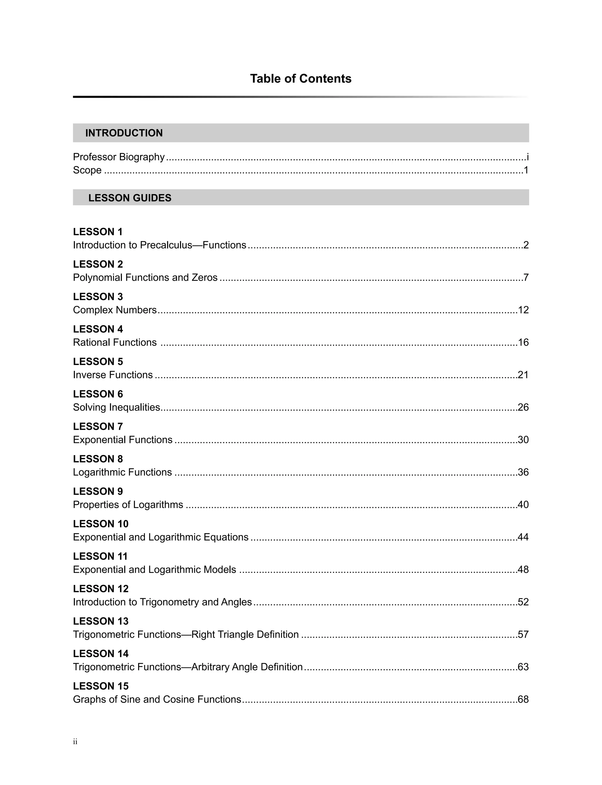
High School
Topic
Mathematics
Subtopic
Course Workbook
Mathematics Describing
the Real World:
Precalculus and Trigonometry
Professor Bruce H. Edwards
University of Florida
Professor Bruce H. Edwards is Professor of Mathematics at the University of Florida, where
he has won a host of awards and recognitions. He was named Teacher of the Year in the
College of Liberal Arts and Sciences and was selected as a Distinguished Alumni Professor
by the Office of Alumni Affairs. Professor Edwards’s coauthored mathematics textbooks
have earned awards from the Text and Academic Authors Association.
PrecalculusandTrigonometryWorkbook](https://image.slidesharecdn.com/precalculusandtrigonometry-201205151455/75/Precalculus-and-trigonometry-1-2048.jpg)

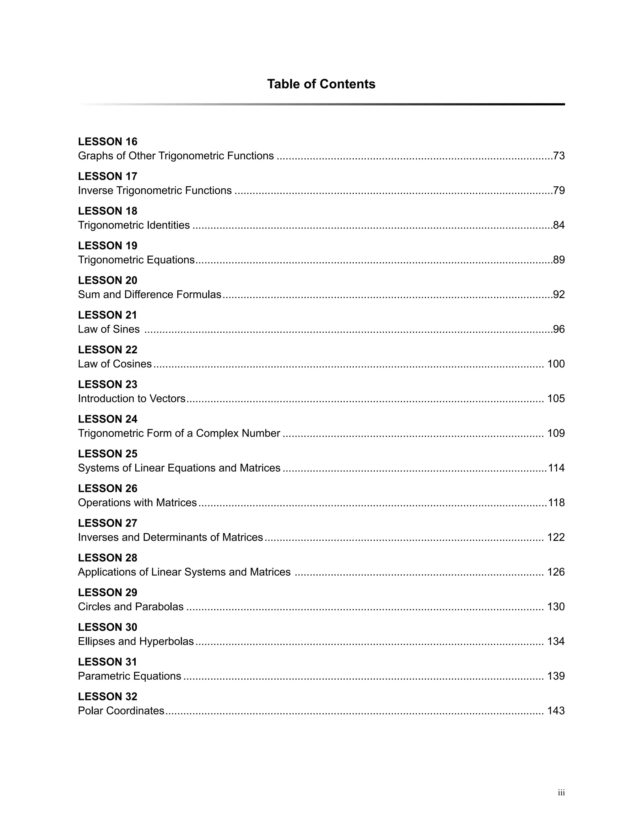


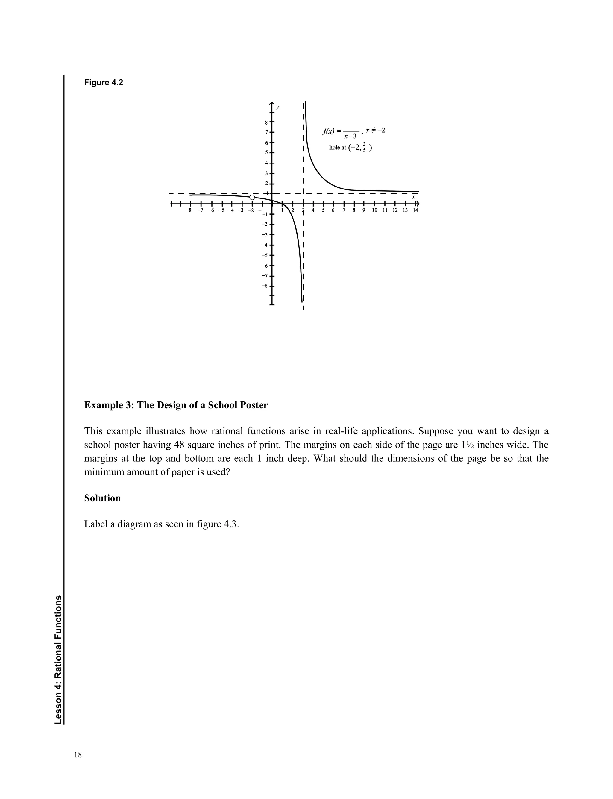


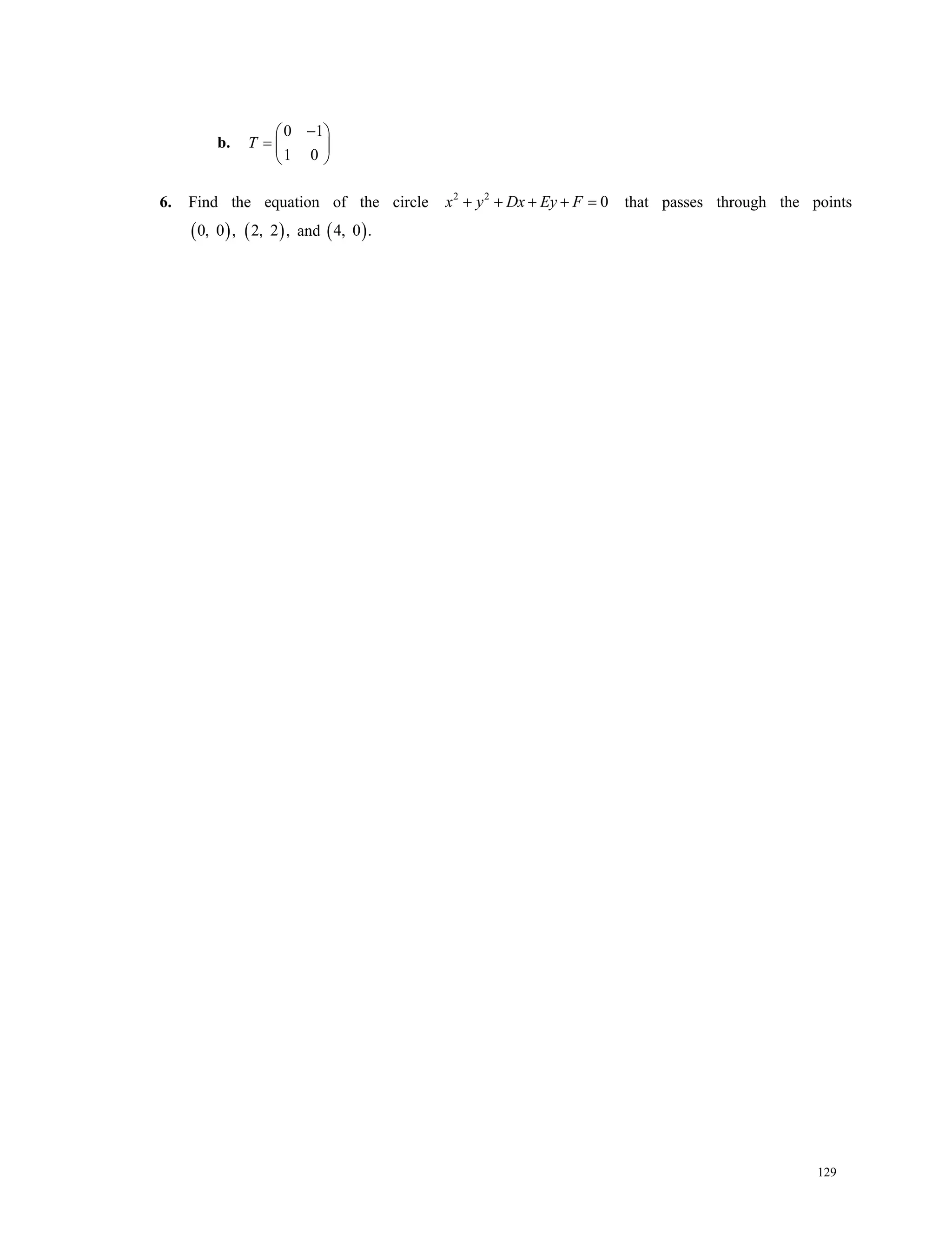


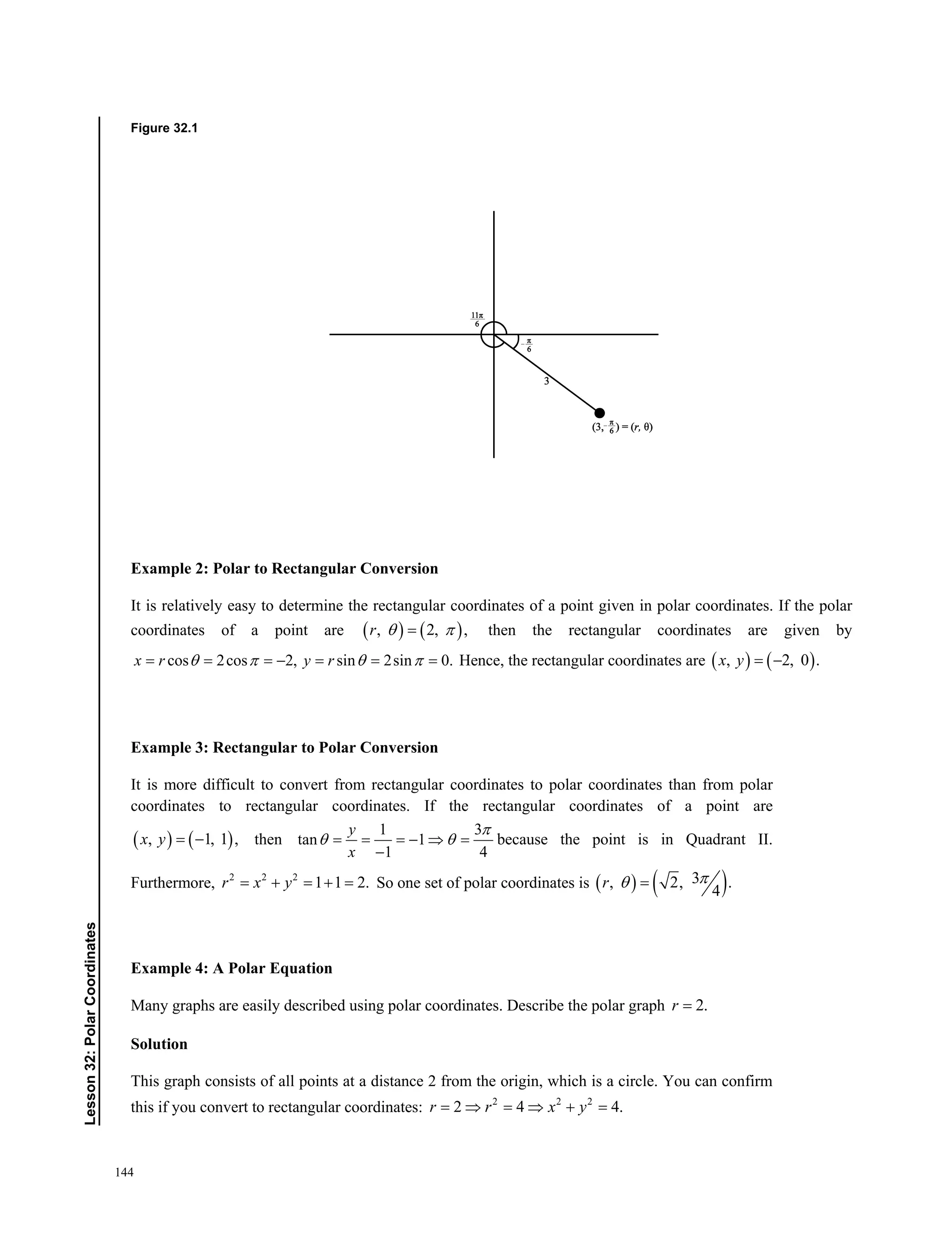


![223
fundamental theorem of algebra (3): If f is a polynomial of degree , 0,n n then f has precisely n linear
factors: ( )( ) ( )1 2( ) ,n nf x a x c x c x c= − − − where 1 2, , nc c c are complex numbers.
Gaussian model (11): ( )2
/
.
x b c
y ae
− −
=
Heron’s area formula (22): A triangle with sides a, b, and c: where .
2
a b c
s
+ +
=
horizontal translations (15): Determined by solving the equations 0bx c− = and 2 .bx c π− =
intermediate value theorem (2): If a and b are real numbers, ,a b and if f is a polynomial function such that
( ) ( ),f a f b≠ then in the interval [ ], ,a b f takes on every value between ( )f a and ( ).f b In particular, if ( )f a
and ( )f b have opposite signs, then f has a zero in the interval [ ], .a b
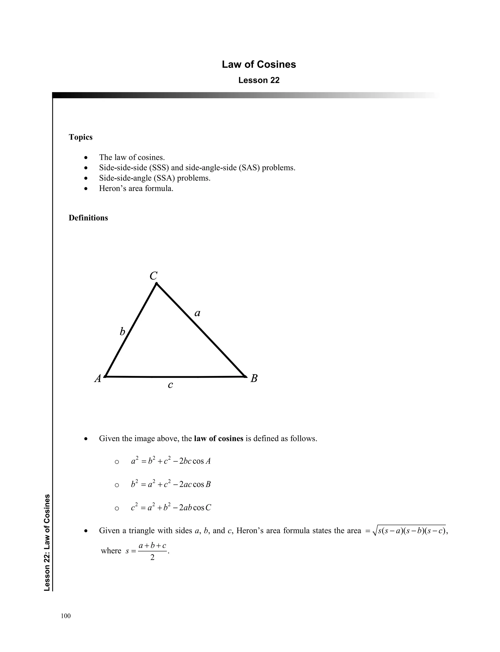
law of cosines (22): 2 2 2 2 2 2 2 2 2
2 cos ; 2 cos ; 2 cos .a b c bc A b a c ac B c a b ab C= + − = + − = + −
law of sines (21): .
sin sin sin
a b c
A B C
= =
linear speed (12): Arc length divided by time: .
s
t
logistic growth model (11): .
1 rx
a
y
be−
=
+
magnitude (or length) of v (23):
matrix inverse algorithm (27): To find the inverse of the n n× square matrix ,A adjoin the n n× identity
matrix and row reduce. If you are able to reduce A to ,I then I will simultaneously reduce to the inverse 1
A−
:
[ ] 1
A I I A−
→ . Otherwise, the matrix A does not have an inverse.
multiplication and division of complex numbers (24): Let ( )1 1 1 1cos sinz r iθ θ= + and ( )2 2 2 2cos sin .z r iθ θ= +
• Multiplication: ( ) ( )1 2 1 2 1 2 1 2cos sin .z z r r iθ θ θ θ= + + +
• Division: ( ) ( )1 1
1 2 1 2 2
2 2
cos sin , 0.
z r
i z
z r
θ θ θ θ= − + − ≠
Newton’s law of cooling (11): The rate of change in the temperature of an object is proportional to the difference
between the object’s temperature and the temperature of the surrounding medium.
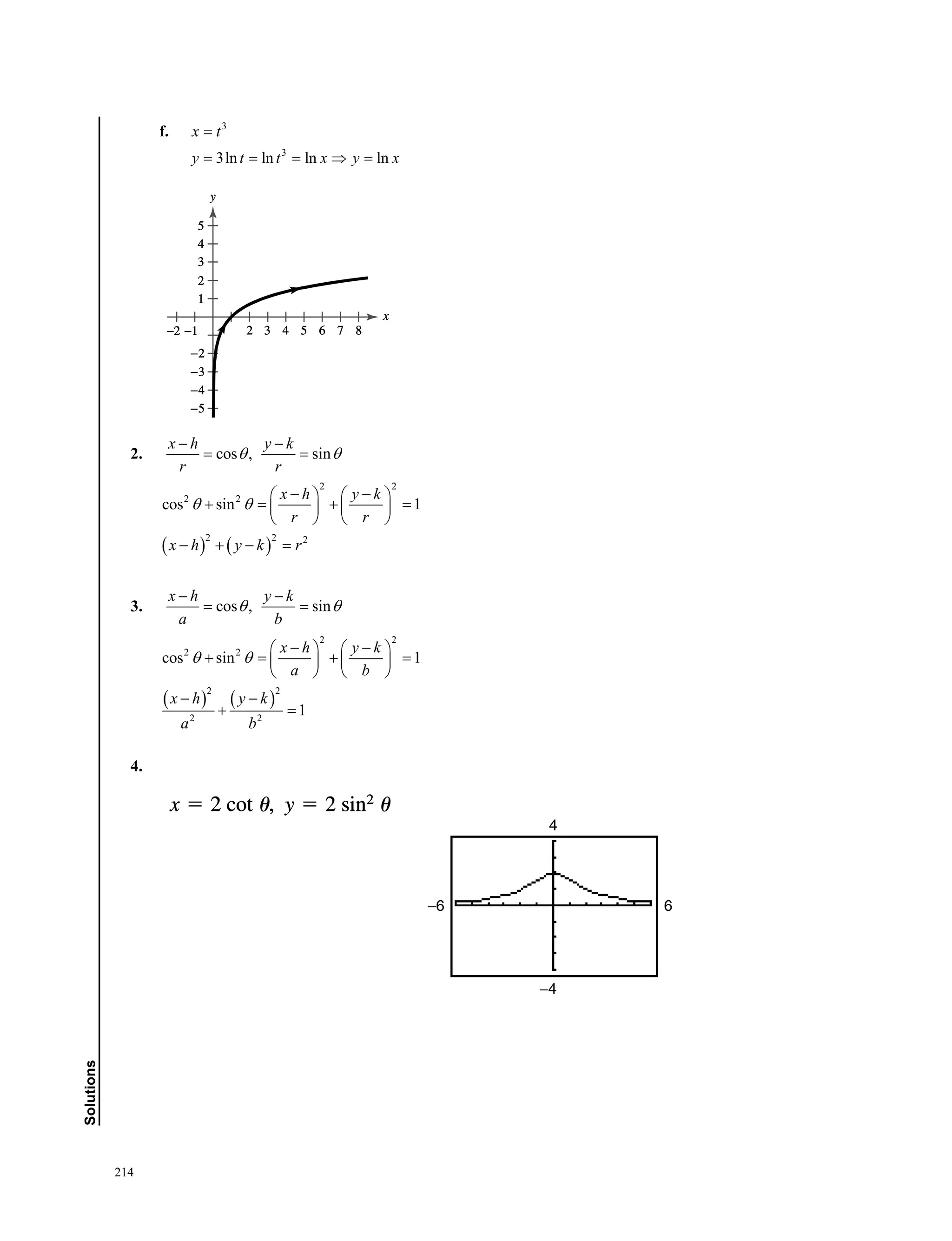
parametric equations (31): The parametric equations of the line through the 2 points ( )1 1,x y and ( )2 2,x y are
( ) ( )1 2 1 1 2 1, .x x t x x y y t y y= + − = + −](https://image.slidesharecdn.com/precalculusandtrigonometry-201205151455/75/Precalculus-and-trigonometry-229-2048.jpg)


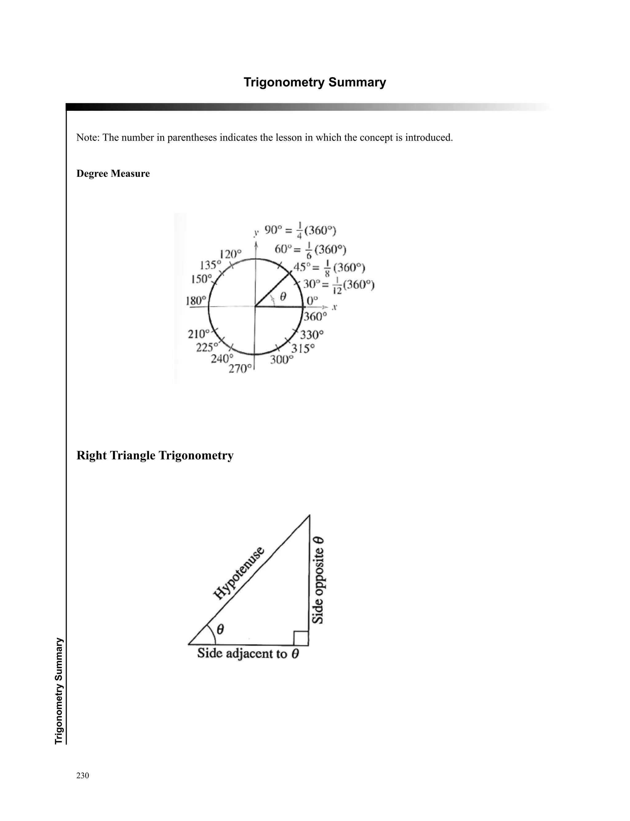


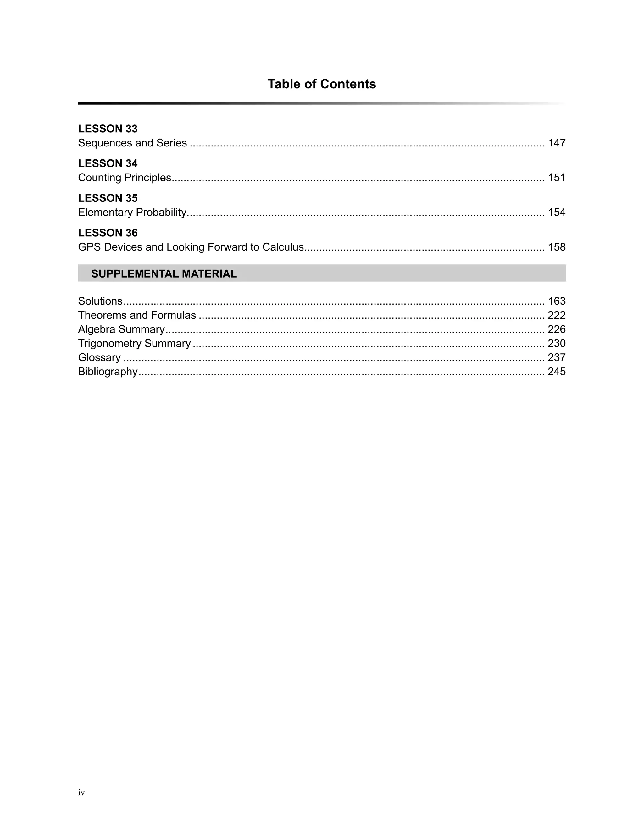
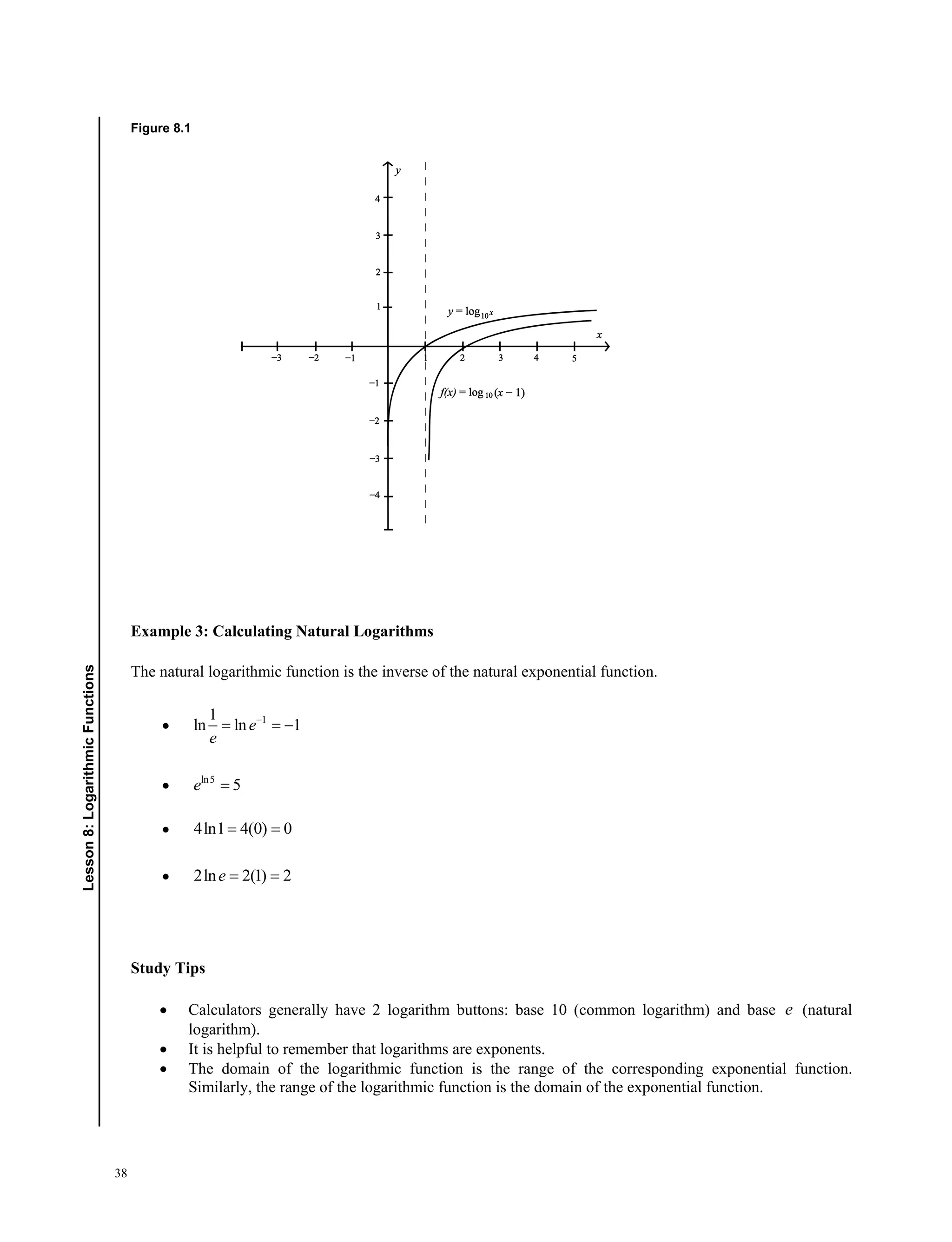
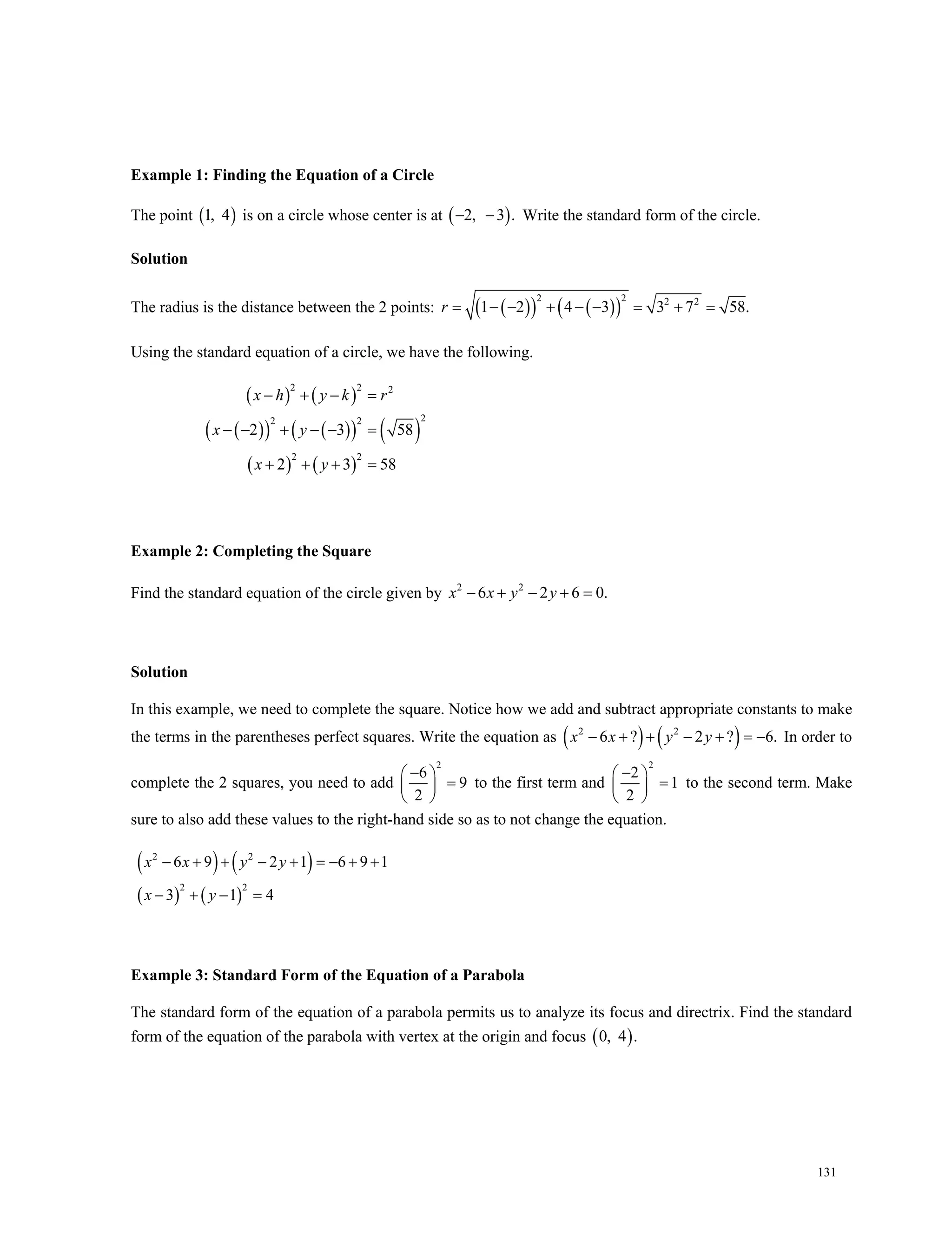
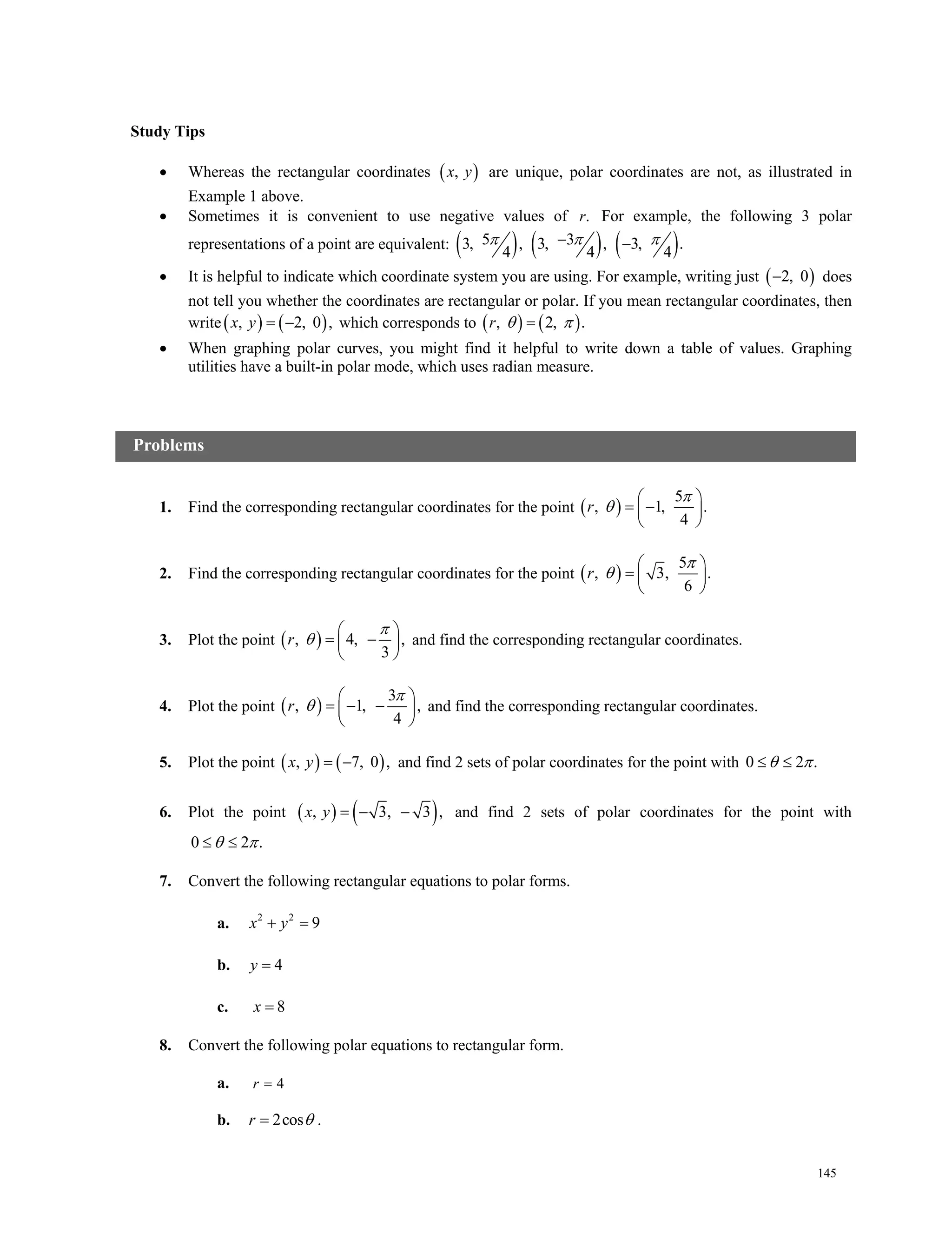
![237
Glossary
Note: The number in parentheses indicates the lesson in which the concept or term is introduced.
absolute value function (1):
, 0
( ) .
, 0
x x
f x x
x x
≥
= =
−
The absolute value of a number is always nonnegative.
absolute value of a complex number (24): See complex numbers.
acute angle (12): An angle between 0° and 90 .°
addition of functions (5): ( )( ) ( ) ( ).f g x f x g x+ = +
amplitude (15): Given the general sine and cosine functions sin( ), cos( ),y d a bx c y d a bx c=+ − =+ − where
b 0, amplitude is .a This number represents half the distance between the maximum and minimum values of
the function.
angle (12): Is determined by rotating a ray (half-line) about its endpoint. The starting position of the ray is the
initial side, and the end position is the terminal side. The endpoint of the ray is the vertex. If the origin is the
vertex and the initial side is the positive x-axis, then the angle is in standard position.
angular speed (12): Measures how fast the angle is changing. It is the central angle divided by time: .
t
θ
axis of a parabola (29): See parabola.
center of a circle (29): See circle.
center of a hyperbola (30): See hyperbola.
center of an ellipse (30): See ellipse.
circle (29): The set of all points ( ),x y in a plane that are equidistant from a fixed point ( ), ,h k called the center
of the circle. The distance between the center and any point ( ),x y on the circle is the radius, r.
closed interval (6): Closed interval [ ],a b means .a x b≤ ≤
common logarithms (8): Logarithms to base 10.
complementary angles (12): Two positive angles are complements of each other if their sum is 90 .°
complement of an event (35): See experiment.
complex conjugate (3): The complex conjugate of a bi+ is .a bi−
complex numbers (3): The set of complex or imaginary numbers consists of all numbers of the form ,a bi+
where a and b are real numbers.
The absolute value or modulus of a complex number a bi+ is 2 2
.a bi a b+ = +](https://image.slidesharecdn.com/precalculusandtrigonometry-201205151455/75/Precalculus-and-trigonometry-243-2048.jpg)


This document provides information about a precalculus and trigonometry workbook created by The Great Courses. It includes a biography of the workbook's author, Professor Bruce H. Edwards of the University of Florida. The workbook is designed to accompany Professor Edwards' Great Courses lecture series on precalculus and contains 30 lesson guides on topics ranging from functions and complex numbers to trigonometric identities, vectors, and conic sections. It is published by The Great Courses, an educational media company located in Chantilly, Virginia.


![[W]-REFERENCIA-Paul Waltman (Auth.) - A Second Course in Elementary Different...](https://cdn.slidesharecdn.com/ss_thumbnails/w-referencia-paulwaltmanauth-230516025940-c93e36a9-thumbnail.jpg?width=640&height=640&fit=bounds)


