OK

1. Random Variables &
Probability Distributions
Sahadeb Sarkar
IIM Calcutta

2. 2
Concept of a Random Variable
A “random variable” is a function which assumes
its values depending on the outcome of an
“experiment” (e.g., survey or just observing).
Thus, a random variable assigns a numerical value
to each of outcomes.

3. 3
Random Variable: Examples
1. Sensex Closing Value on next trading day,
2. Quarterly Sales (Profit) of Wipro,
3. Average PE for Indian Banks,
4. Number of items of a product in inventory,
5. Gold Price,
6. Dollar/Euro Exchange Rate,
7. Amount of Insurance Claims in a Month,
8. Annual Return on a Stock
9. Waiting Time at a Check-out Counter

4. 4
Example
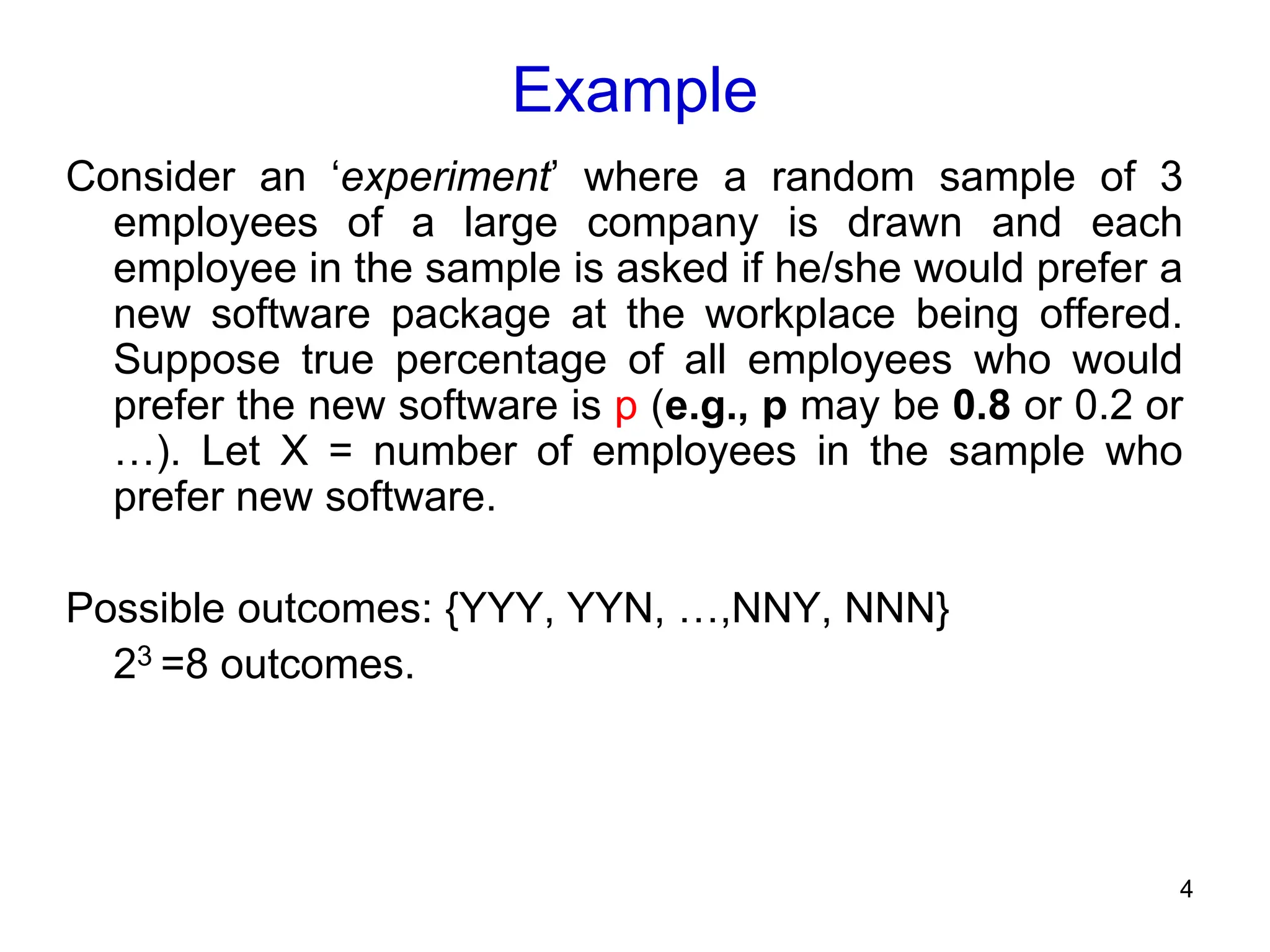
Consider an ‘experiment’ where a random sample of 3
employees of a large company is drawn and each
employee in the sample is asked if he/she would prefer a
new software package at the workplace being offered.
Suppose true percentage of all employees who would
prefer the new software is p (e.g., p may be 0.8 or 0.2 or
…). Let X = number of employees in the sample who
prefer new software.
Possible outcomes: {YYY, YYN, …,NNY, NNN}
23 =8 outcomes.

5. 5
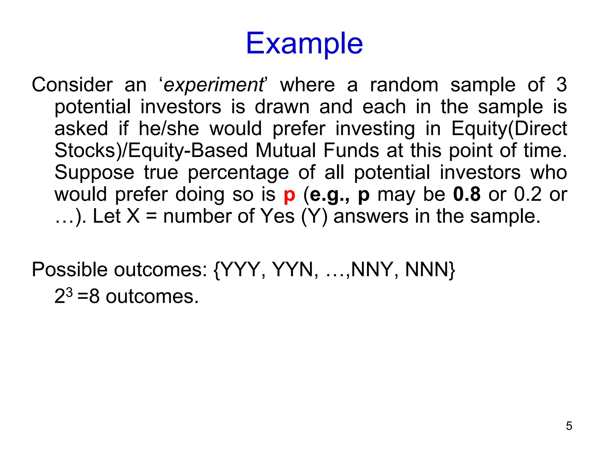
Example
Consider an ‘experiment’ where a random sample of 3
potential investors is drawn and each in the sample is
asked if he/she would prefer investing in Equity(Direct
Stocks)/Equity-Based Mutual Funds at this point of time.
Suppose true percentage of all potential investors who
would prefer doing so is p (e.g., p may be 0.8 or 0.2 or
…). Let X = number of Yes (Y) answers in the sample.
Possible outcomes: {YYY, YYN, …,NNY, NNN}
23 =8 outcomes.

6. 6
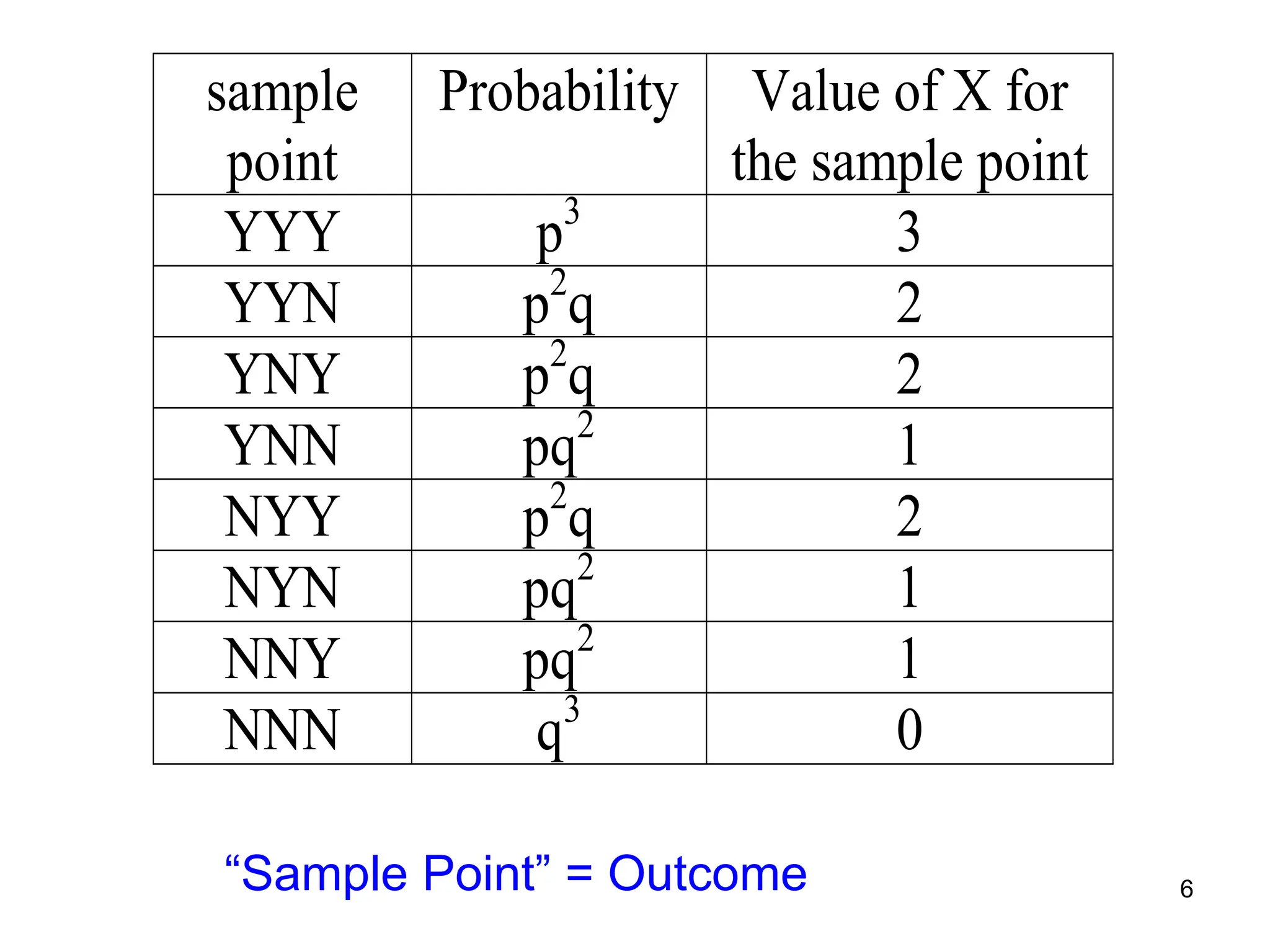
sample
point
Probability Value of X for
the sample point
YYY p3
3
YYN p2
q 2
YNY p2
q 2
YNN pq2
1
NYY p2
q 2
NYN pq2
1
NNY pq2
1
NNN q3
0
“Sample Point” = Outcome

7. 7
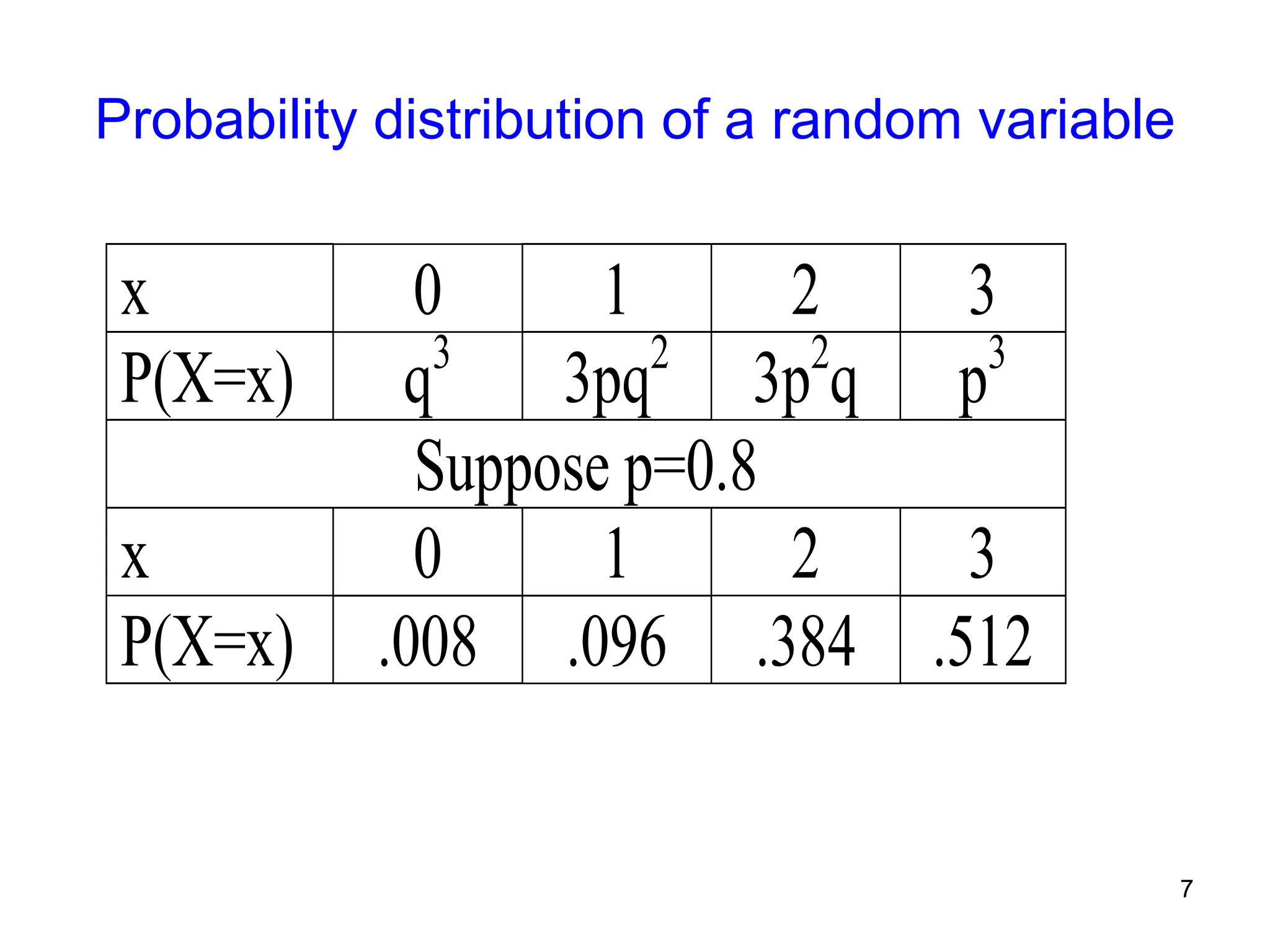
Probability distribution of a random variable
x 0 1 2 3
P(X=x) q3
3pq2
3p2
q p3
Suppose p=0.8
x 0 1 2 3
P(X=x) .008 .096 .384 .512

8. 8
Types of random variables
Discrete r.v.: If its number of possible values is finite
or countably infinite [e.g., {0,1,2,3,…} ]
Usually arises out of counting
e.g., number of items of a product in inventory,
monthly insurance claims, daily number of trades
for a stock, number of customers visiting a store
Continuous r.v.: If it takes values on a continuous
scale.
Usually arises while measuring certain things,
e.g., Investment Return, P/E, lifetime, waiting
time, execution time of a project

9. 9
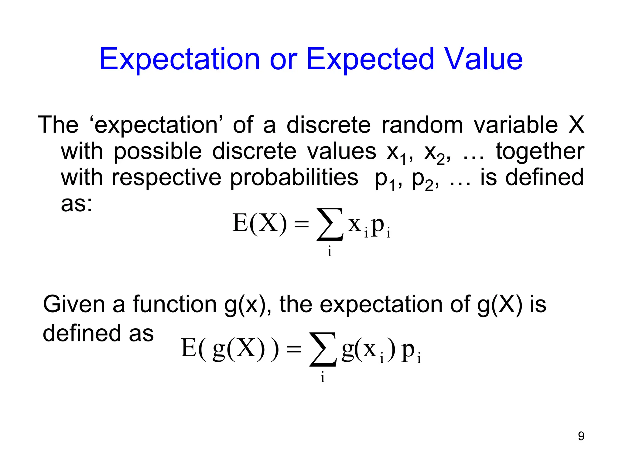
Expectation or Expected Value
The ‘expectation’ of a discrete random variable X
with possible discrete values x1, x2, … together
with respective probabilities p1, p2, … is defined
as:
Given a function g(x), the expectation of g(X) is
defined as


i
i
i p
x
)
X
(
E


i
i
i p
)
g(x
)
)
X
(
g
(
E

10. 10
Number of
items sold, x p(x) xp(x) g(x) g(x)p(x)
5000 0.2 1000 2000 400
6000 0.3 1800 4000 1200
7000 0.2 1400 6000 1200
8000 0.2 1600 8000 1600
9000 0.1 900 10000 1000
1.0 6700 5400
Monthly number (X) of items sold for a certain product are believed
to follow the given probability distribution. Suppose the company
has a fixed monthly production cost of 8000 units of money and that
each item brings 2 units of money. Find expected monthly number
of items sold & expected monthly profit g(X), from product sales.
5400
)
x
(
p
)
x
(
g
)]
X
(
g
[
E
Profit
Monthly
Expected
x


 
Here, E(X)= 5000*.2 +6000*.3 + 7000*.2 + 8000*.2 + 9000*.1 = 6700
Computation of Expectation
Profit g (X) = 2X – 8000 where X = # of items sold

11. 11
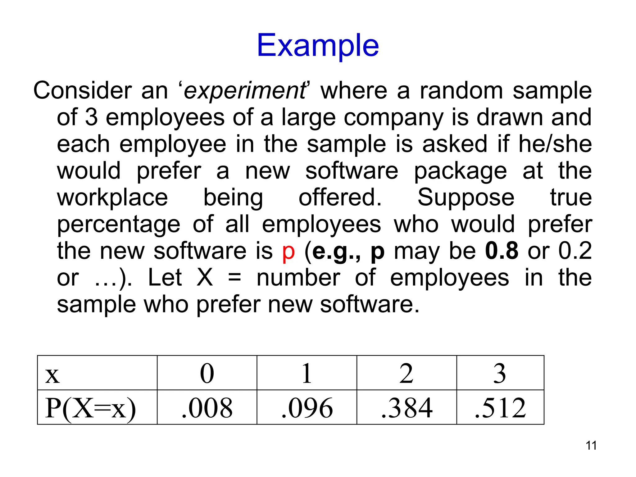
Example
Consider an ‘experiment’ where a random sample
of 3 employees of a large company is drawn and
each employee in the sample is asked if he/she
would prefer a new software package at the
workplace being offered. Suppose true
percentage of all employees who would prefer
the new software is p (e.g., p may be 0.8 or 0.2
or …). Let X = number of employees in the
sample who prefer new software.
x 0 1 2 3
P(X=x) .008 .096 .384 .512

12. 12
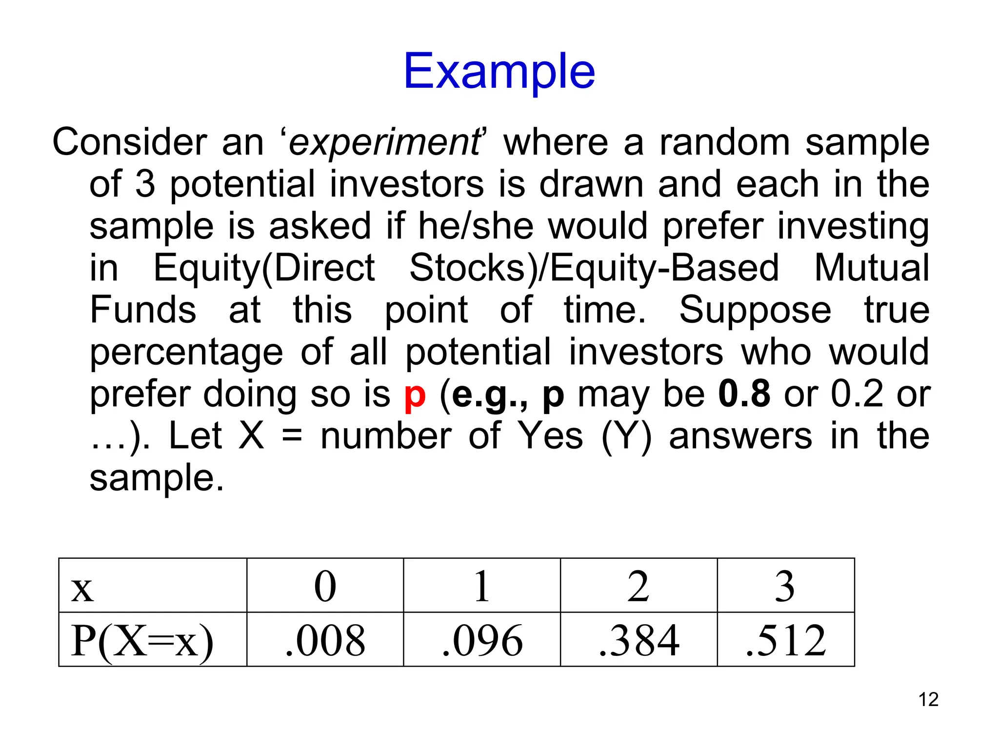
Example
Consider an ‘experiment’ where a random sample
of 3 potential investors is drawn and each in the
sample is asked if he/she would prefer investing
in Equity(Direct Stocks)/Equity-Based Mutual
Funds at this point of time. Suppose true
percentage of all potential investors who would
prefer doing so is p (e.g., p may be 0.8 or 0.2 or
…). Let X = number of Yes (Y) answers in the
sample.
x 0 1 2 3
P(X=x) .008 .096 .384 .512

13. 13
Example
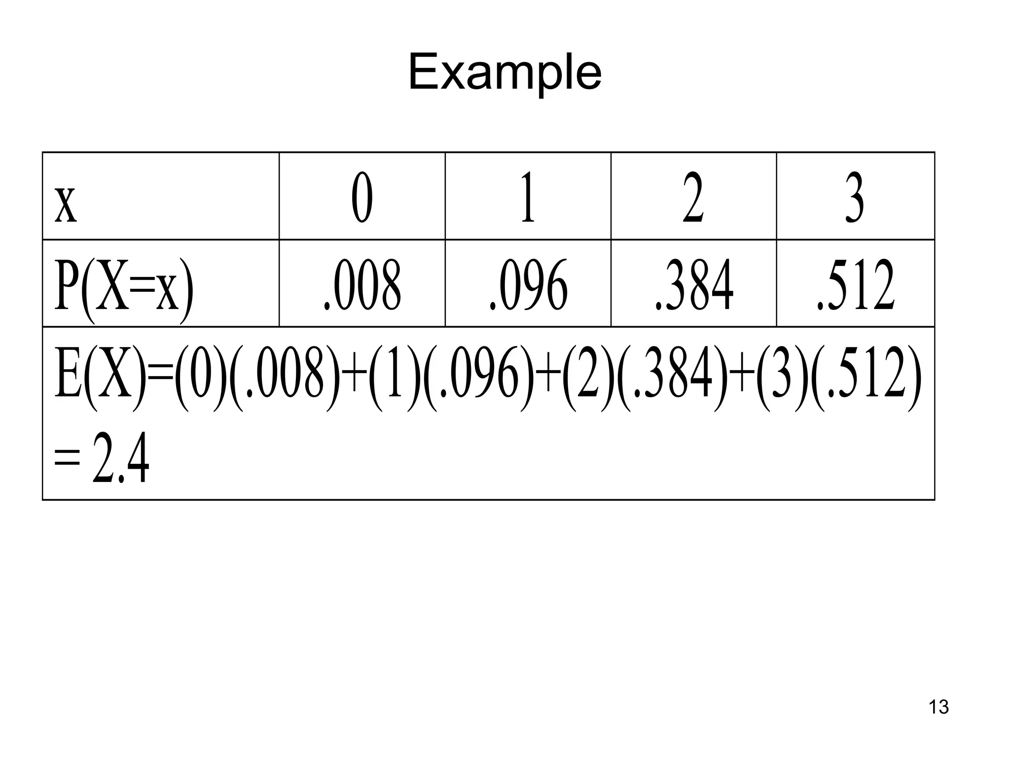
x 0 1 2 3
P(X=x) .008 .096 .384 .512
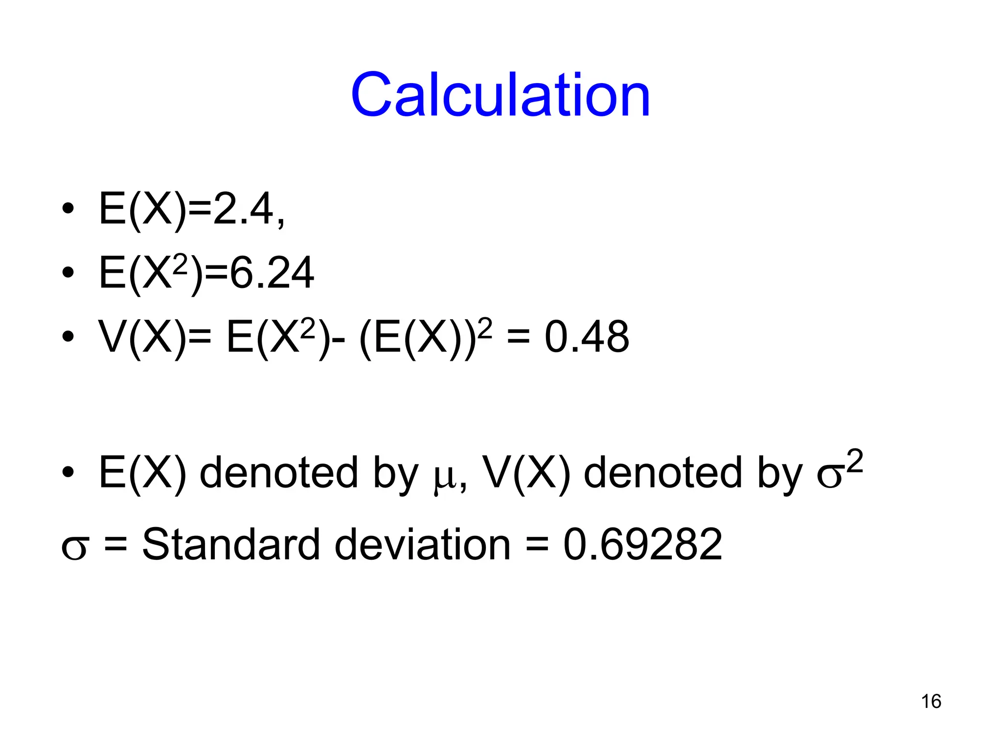
E(X)=(0)(.008)+(1)(.096)+(2)(.384)+(3)(.512)
= 2.4

14. 14
Variance
Definition: Variance of a random variable X is defined as:
2 = V (X) = E [(X-E(X))2 ] = E(X2) – (E(X))2,
For a dataset X1, X2, …, Xn, sample variance is equal to
average of squared Xi values minus square of the average
of the Xi values, as shown below:
• 𝒔𝒏
𝟐 =
1
𝑛−1 𝑖=1
𝑛
𝑋𝑖 − 𝑋 2 =
n
𝑛−1
1
𝑛 𝑖=1
𝑛
𝑋𝑖 − 𝑋 2 =
n
𝑛−1
1
𝑛 𝑖=1
𝑛
𝑋𝑖
2
 𝑛𝑋2
• =
n
𝑛−1
𝟏
𝒏 𝒊=𝟏
𝒏
𝑿𝒊
𝟐
 𝑿𝟐  (1)
1
𝑛 𝑖=1
𝑛
𝑋𝑖
2
 𝑋2 =
"𝑬(𝑿𝟐) − (𝑬(𝑿))𝟐". ]

15. 15
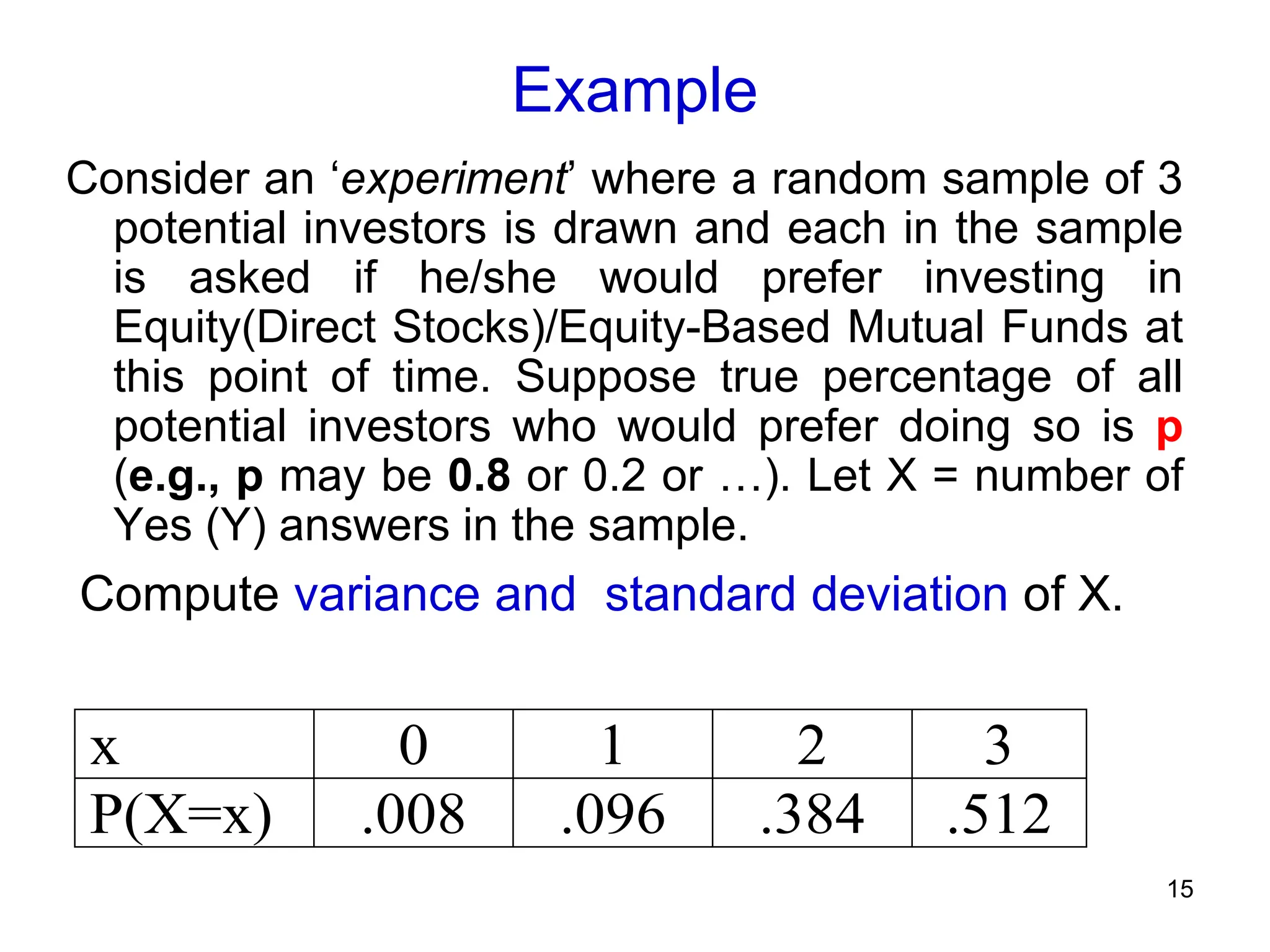
Example
Consider an ‘experiment’ where a random sample of 3
potential investors is drawn and each in the sample
is asked if he/she would prefer investing in
Equity(Direct Stocks)/Equity-Based Mutual Funds at
this point of time. Suppose true percentage of all
potential investors who would prefer doing so is p
(e.g., p may be 0.8 or 0.2 or …). Let X = number of
Yes (Y) answers in the sample.
Compute variance and standard deviation of X.
x 0 1 2 3
P(X=x) .008 .096 .384 .512

16. 16
Calculation
• E(X)=2.4,
• E(X2)=6.24
• V(X)= E(X2)- (E(X))2 = 0.48
• E(X) denoted by , V(X) denoted by 2
 = Standard deviation = 0.69282

17. 17
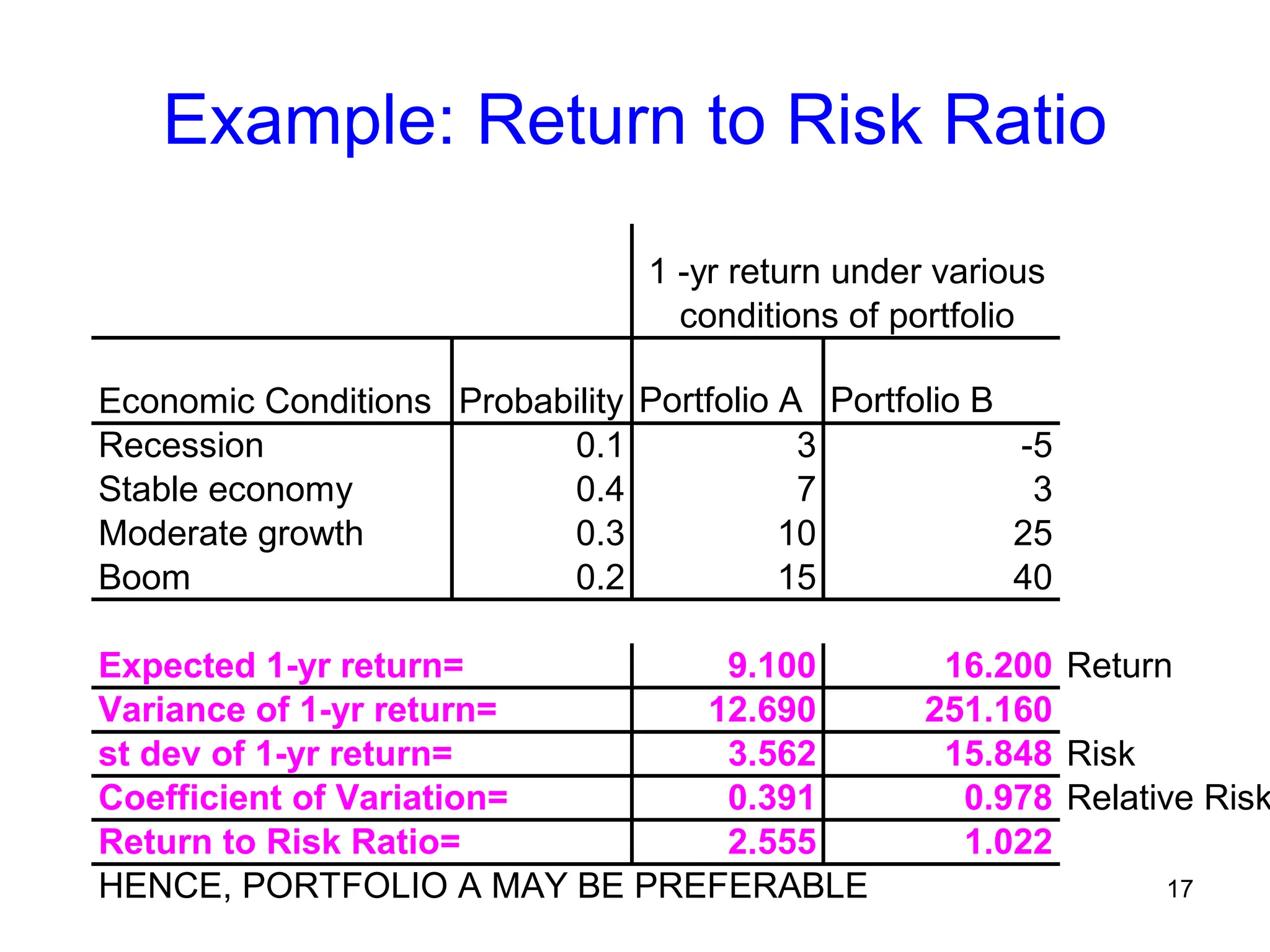
Example: Return to Risk Ratio
Economic Conditions Probability Portfolio A Portfolio B
Recession 0.1 3 -5
Stable economy 0.4 7 3
Moderate growth 0.3 10 25
Boom 0.2 15 40
Expected 1-yr return= 9.100 16.200 Return
Variance of 1-yr return= 12.690 251.160
st dev of 1-yr return= 3.562 15.848 Risk
Coefficient of Variation= 0.391 0.978 Relative Risk
Return to Risk Ratio= 2.555 1.022
HENCE, PORTFOLIO A MAY BE PREFERABLE
1 -yr return under various
conditions of portfolio

18. 18
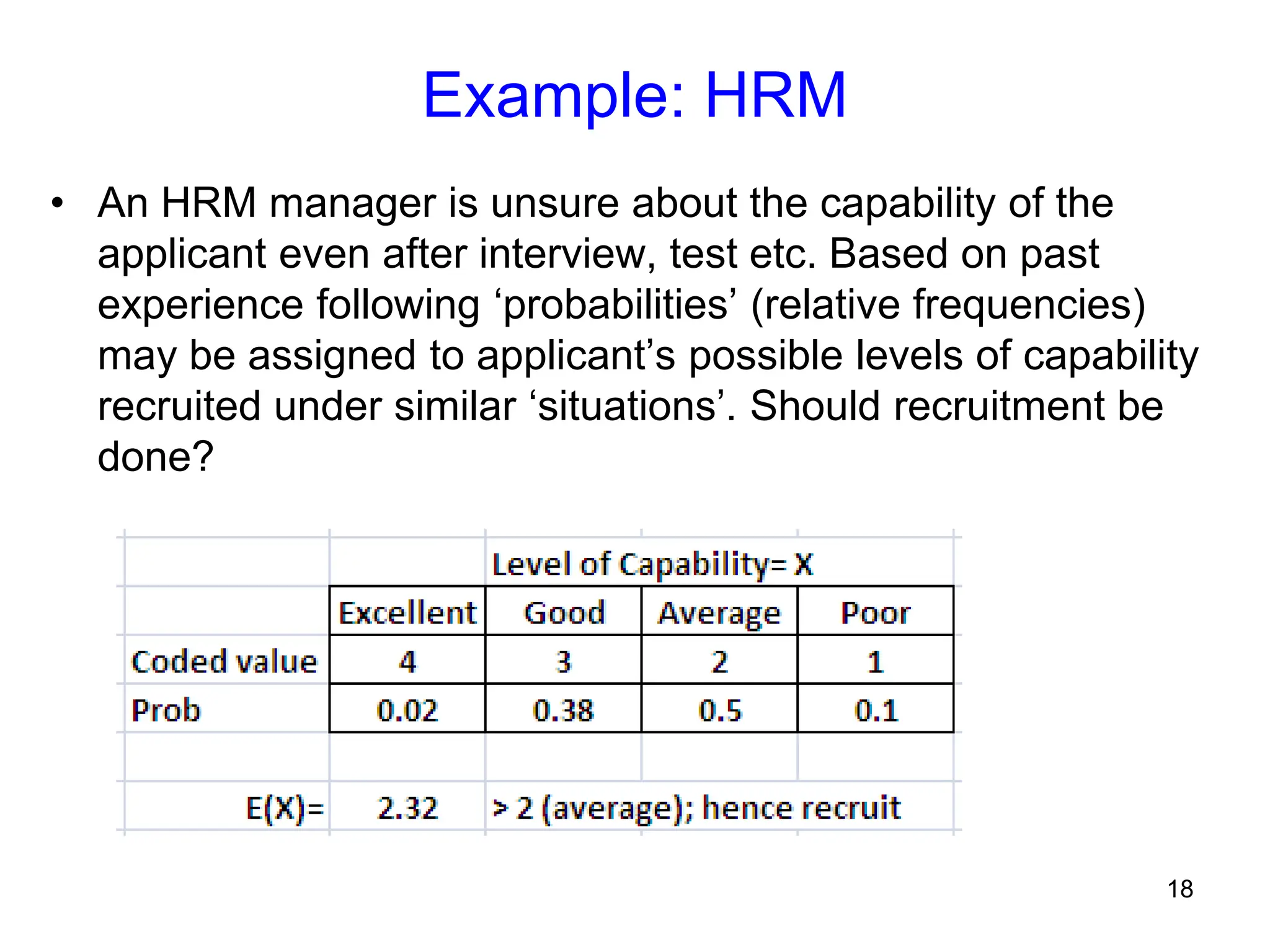
Example: HRM
• An HRM manager is unsure about the capability of the
applicant even after interview, test etc. Based on past
experience following ‘probabilities’ (relative frequencies)
may be assigned to applicant’s possible levels of capability
recruited under similar ‘situations’. Should recruitment be
done?

19. 19
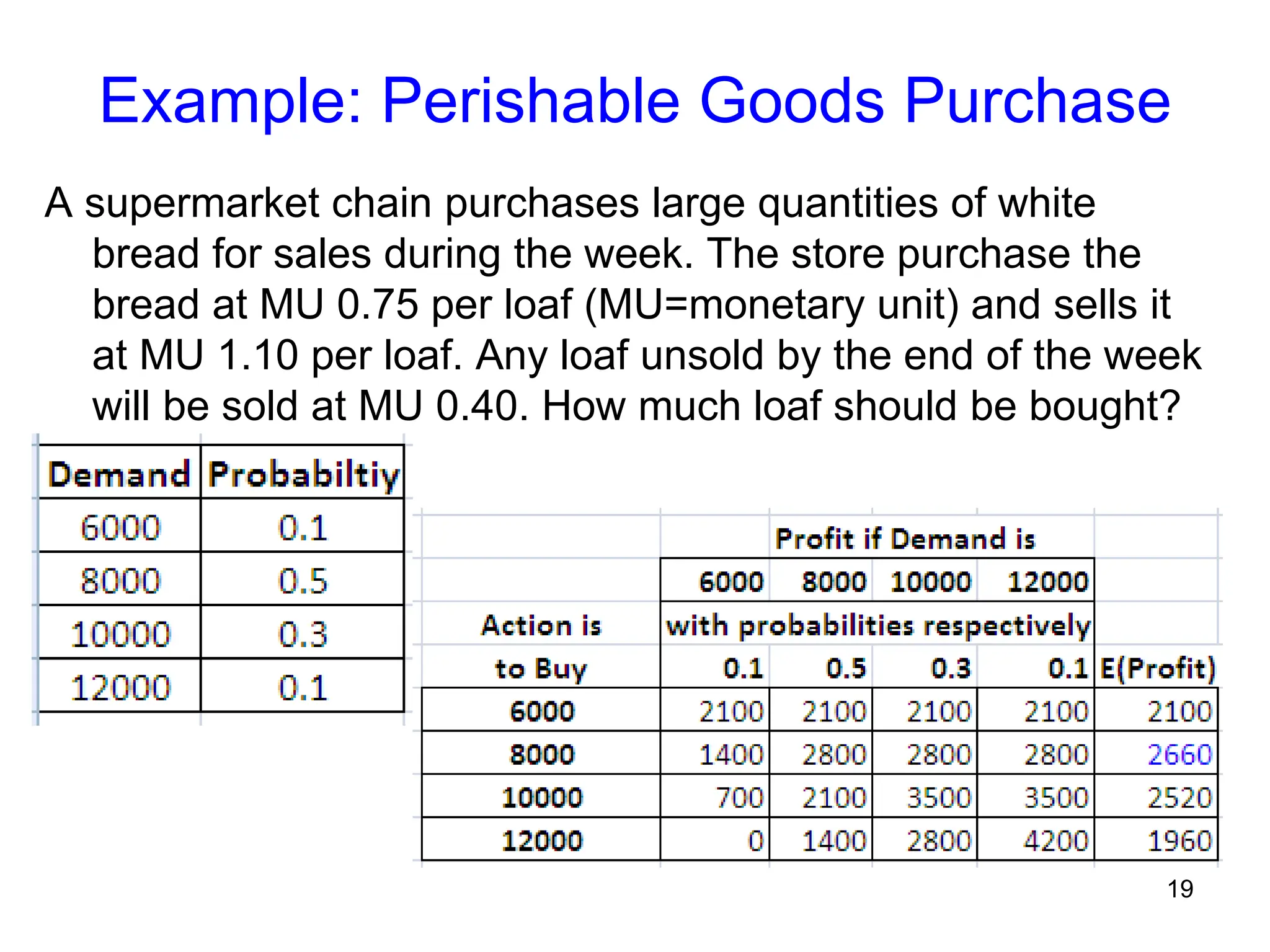
Example: Perishable Goods Purchase
A supermarket chain purchases large quantities of white
bread for sales during the week. The store purchase the
bread at MU 0.75 per loaf (MU=monetary unit) and sells it
at MU 1.10 per loaf. Any loaf unsold by the end of the week
will be sold at MU 0.40. How much loaf should be bought?

20. 20
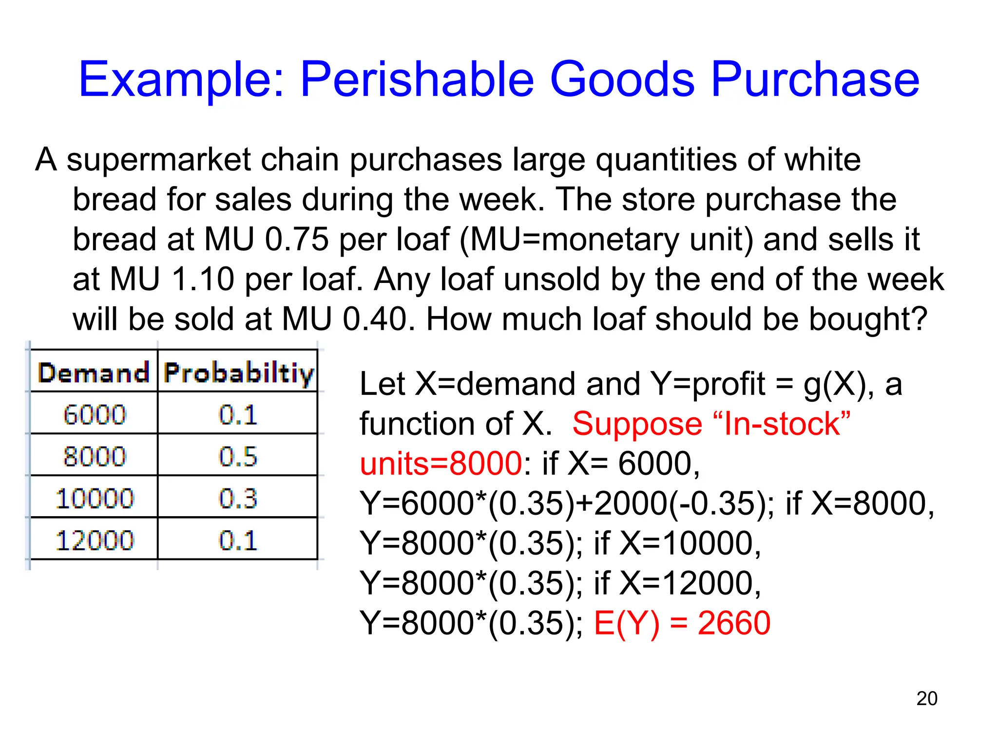
Example: Perishable Goods Purchase
A supermarket chain purchases large quantities of white
bread for sales during the week. The store purchase the
bread at MU 0.75 per loaf (MU=monetary unit) and sells it
at MU 1.10 per loaf. Any loaf unsold by the end of the week
will be sold at MU 0.40. How much loaf should be bought?
Let X=demand and Y=profit = g(X), a
function of X. Suppose “In-stock”
units=8000: if X= 6000,
Y=6000*(0.35)+2000(-0.35); if X=8000,
Y=8000*(0.35); if X=10000,
Y=8000*(0.35); if X=12000,
Y=8000*(0.35); E(Y) = 2660

21. 21
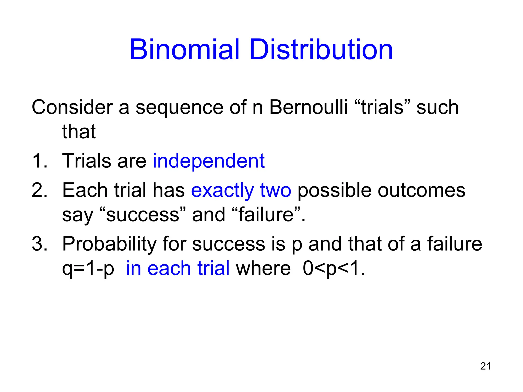
Binomial Distribution
Consider a sequence of n Bernoulli “trials” such
that
1. Trials are independent
2. Each trial has exactly two possible outcomes
say “success” and “failure”.
3. Probability for success is p and that of a failure
q=1-p in each trial where 0<p<1.

22. 22
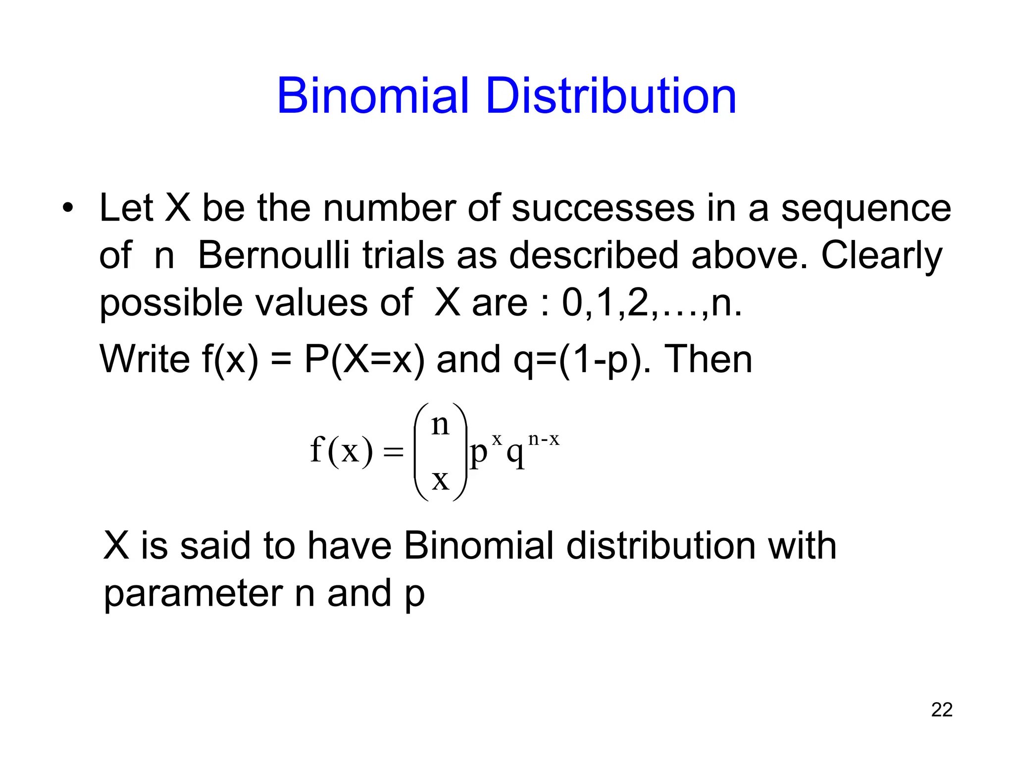
Binomial Distribution
• Let X be the number of successes in a sequence
of n Bernoulli trials as described above. Clearly
possible values of X are : 0,1,2,…,n.
Write f(x) = P(X=x) and q=(1-p). Then
x
-
n
x
q
p
x
n
)
x
(
f 








X is said to have Binomial distribution with
parameter n and p

23. 23
Mean and variance of Bin(n,p) r.v.
Expected value of a Bin(n,p) r.v. is = np
Variance of a Bin(n,p) r.v. is = np(1-p)

24. 24
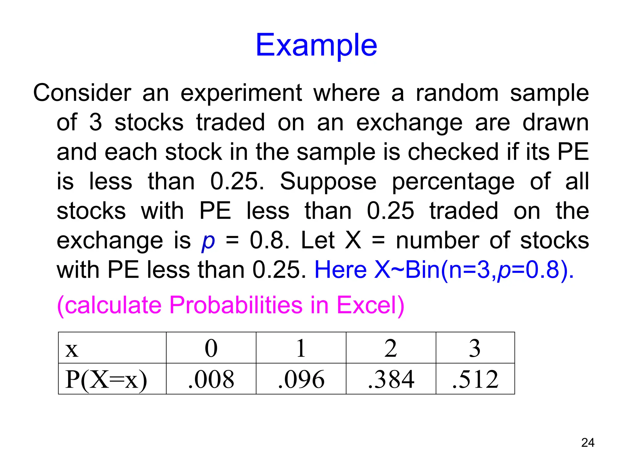
Example
Consider an experiment where a random sample
of 3 stocks traded on an exchange are drawn
and each stock in the sample is checked if its PE
is less than 0.25. Suppose percentage of all
stocks with PE less than 0.25 traded on the
exchange is p = 0.8. Let X = number of stocks
with PE less than 0.25. Here X~Bin(n=3,p=0.8).
(calculate Probabilities in Excel)
x 0 1 2 3
P(X=x) .008 .096 .384 .512

25. 25
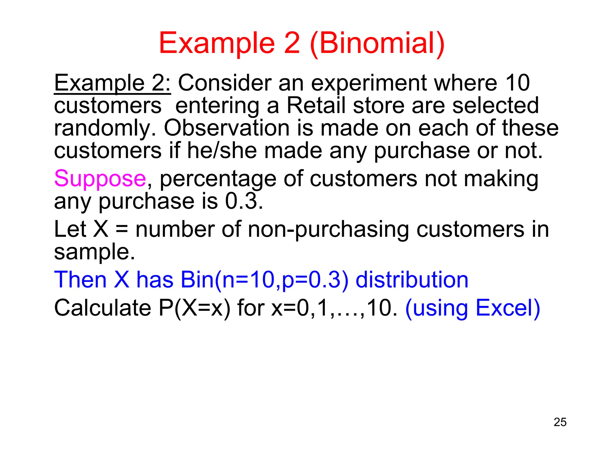
Example 2 (Binomial)
Example 2: Consider an experiment where 10
customers entering a Retail store are selected
randomly. Observation is made on each of these
customers if he/she made any purchase or not.
Suppose, percentage of customers not making
any purchase is 0.3.
Let X = number of non-purchasing customers in
sample.
Then X has Bin(n=10,p=0.3) distribution
Calculate P(X=x) for x=0,1,…,10. (using Excel)

26. 26
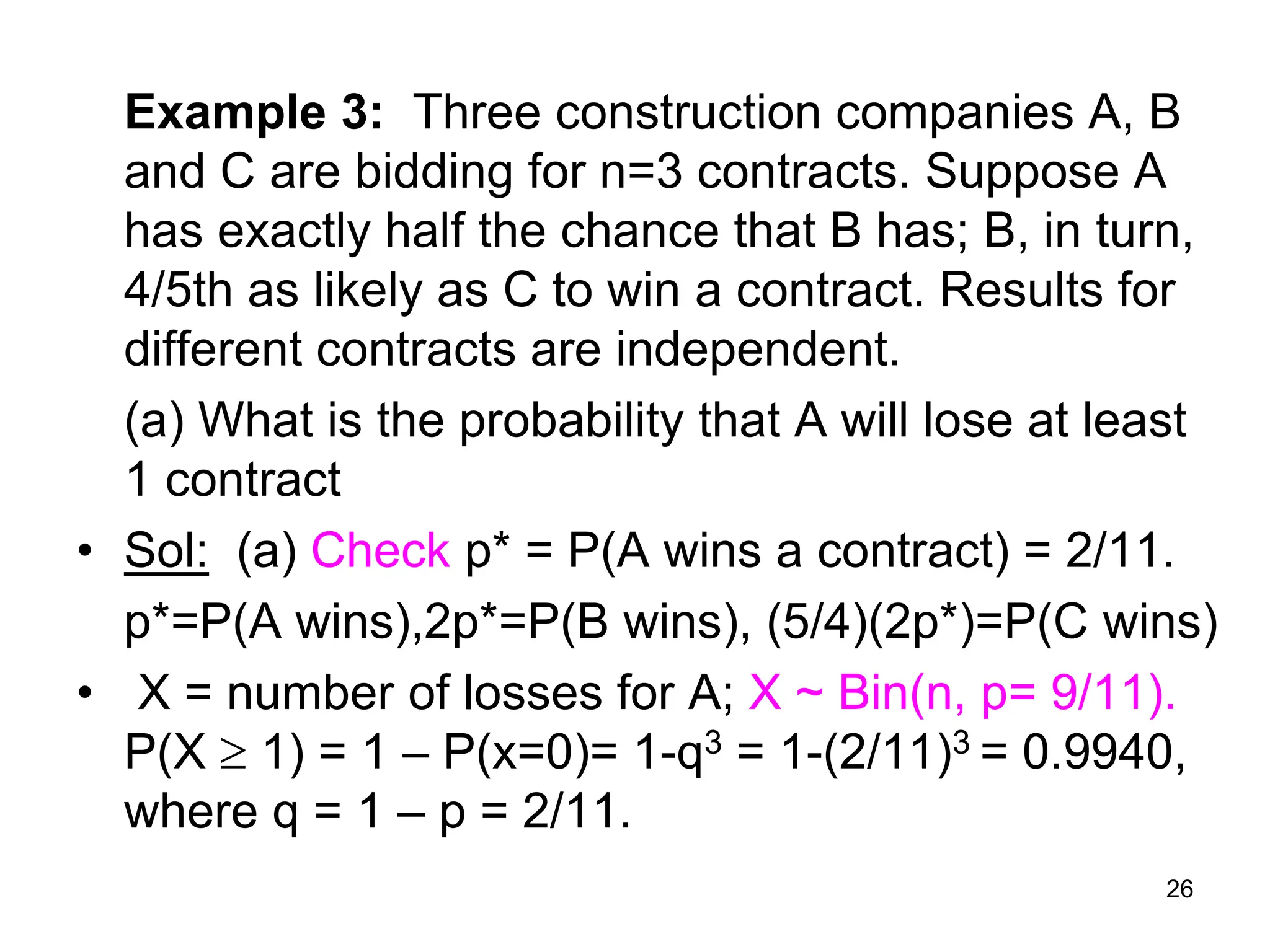
Example 3: Three construction companies A, B
and C are bidding for n=3 contracts. Suppose A
has exactly half the chance that B has; B, in turn,
4/5th as likely as C to win a contract. Results for
different contracts are independent.
(a) What is the probability that A will lose at least
1 contract
• Sol: (a) Check p* = P(A wins a contract) = 2/11.
p*=P(A wins),2p*=P(B wins), (5/4)(2p*)=P(C wins)
• X = number of losses for A; X ~ Bin(n, p= 9/11).
P(X  1) = 1  P(x=0)= 1-q3 = 1-(2/11)3 = 0.9940,
where q = 1 – p = 2/11.

27. 27
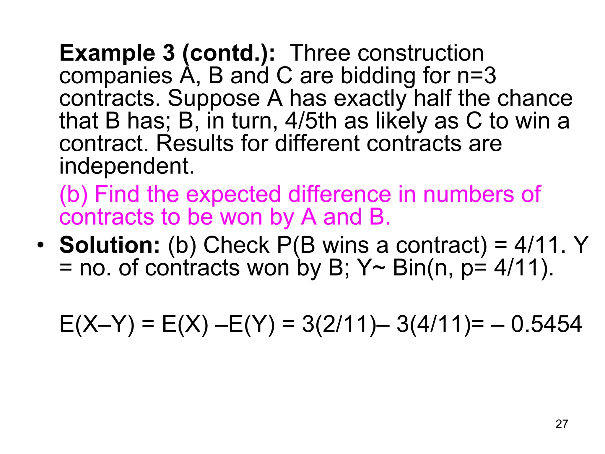
Example 3 (contd.): Three construction
companies A, B and C are bidding for n=3
contracts. Suppose A has exactly half the chance
that B has; B, in turn, 4/5th as likely as C to win a
contract. Results for different contracts are
independent.
(b) Find the expected difference in numbers of
contracts to be won by A and B.
• Solution: (b) Check P(B wins a contract) = 4/11. Y
= no. of contracts won by B; Y~ Bin(n, p= 4/11).
E(XY) = E(X) E(Y) = 3(2/11)– 3(4/11)= – 0.5454

28. 28
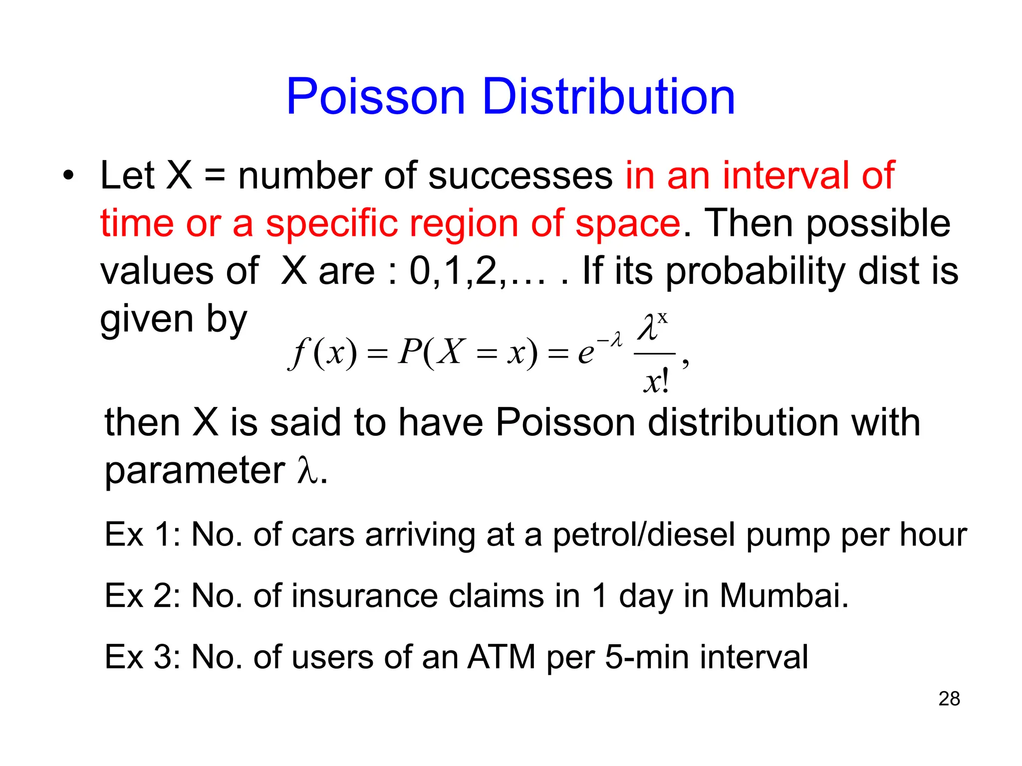
Poisson Distribution
• Let X = number of successes in an interval of
time or a specific region of space. Then possible
values of X are : 0,1,2,… . If its probability dist is
given by
then X is said to have Poisson distribution with
parameter .
Ex 1: No. of cars arriving at a petrol/diesel pump per hour
Ex 2: No. of insurance claims in 1 day in Mumbai.
Ex 3: No. of users of an ATM per 5-min interval
,
!
)
(
)
(
x
x
e
x
X
P
x
f







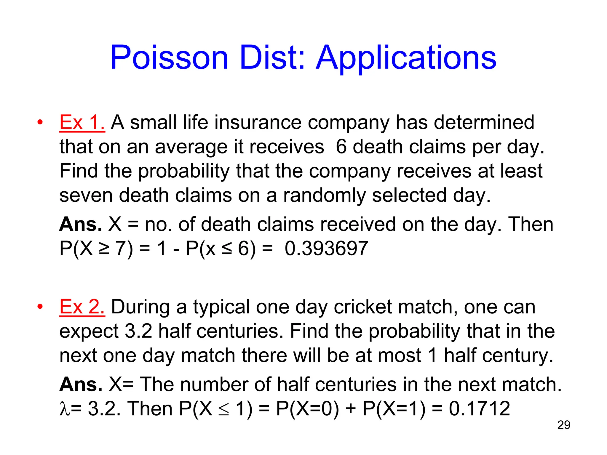
29. Poisson Dist: Applications
• Ex 1. A small life insurance company has determined
that on an average it receives 6 death claims per day.
Find the probability that the company receives at least
seven death claims on a randomly selected day.
Ans. X = no. of death claims received on the day. Then
P(X ≥ 7) = 1 - P(x ≤ 6) = 0.393697
• Ex 2. During a typical one day cricket match, one can
expect 3.2 half centuries. Find the probability that in the
next one day match there will be at most 1 half century.
Ans. X= The number of half centuries in the next match.
= 3.2. Then P(X  1) = P(X=0) + P(X=1) = 0.1712
29

30. 30
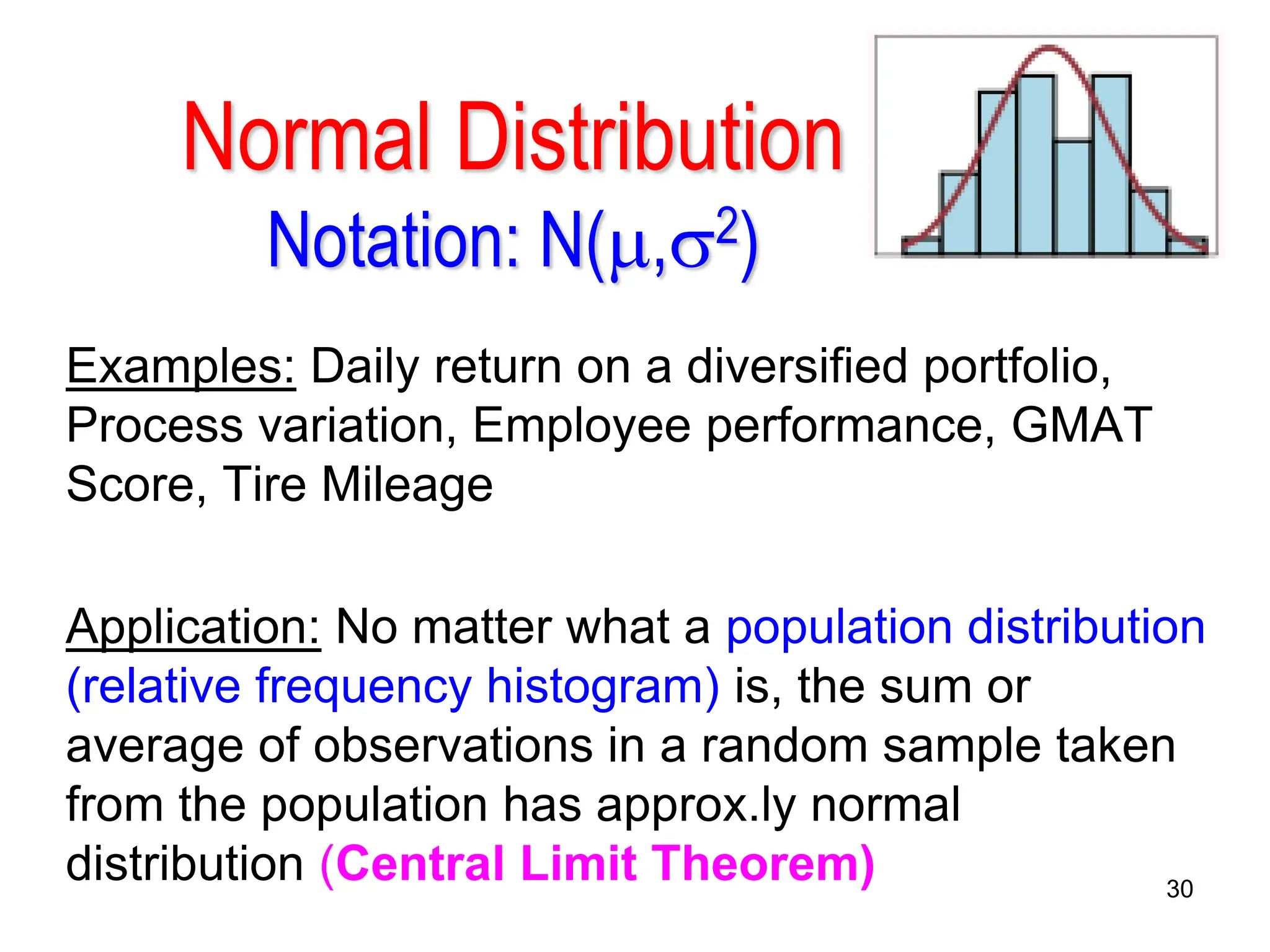
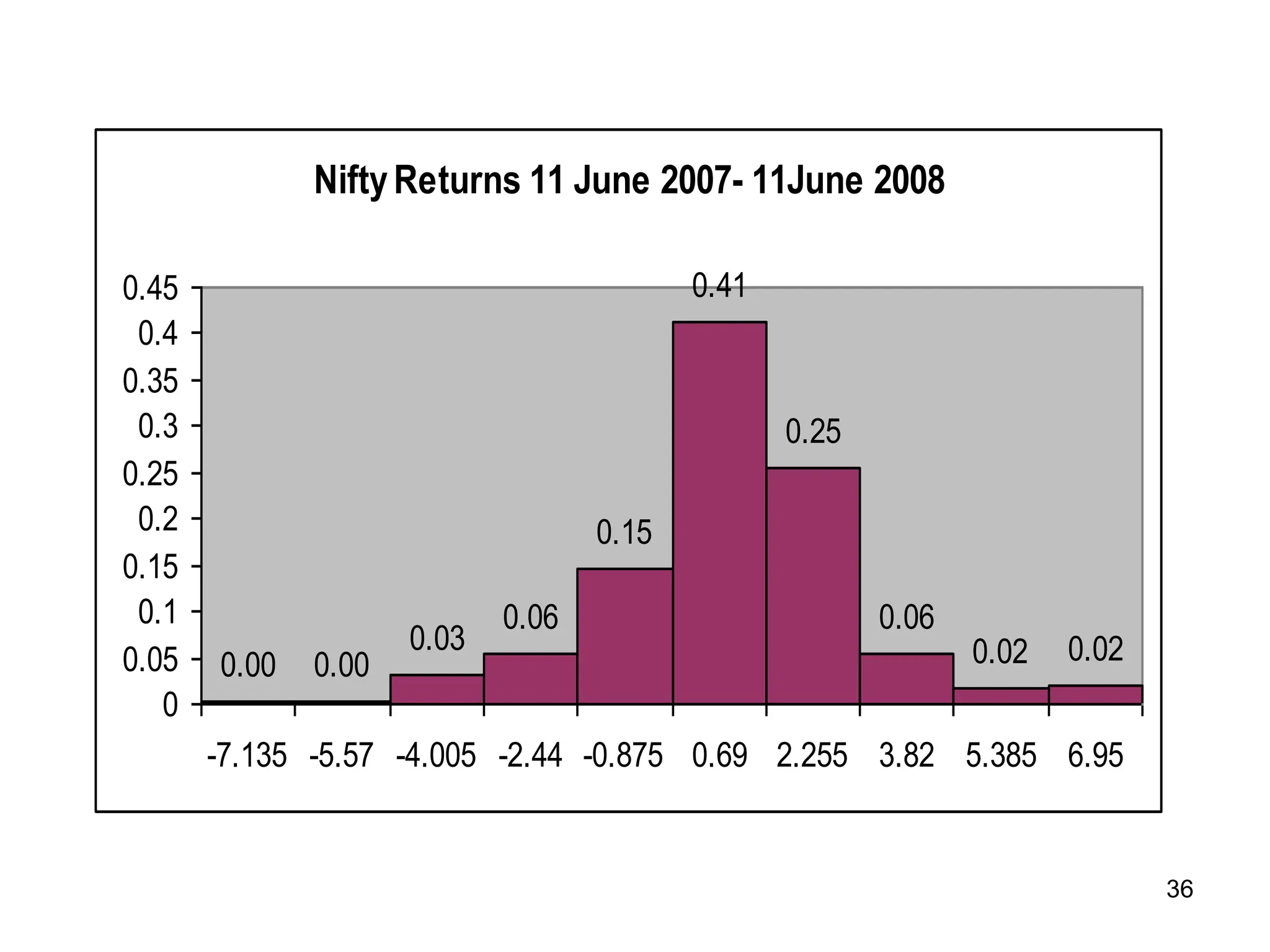
Normal Distribution
Notation: N(,2)
Examples: Daily return on a diversified portfolio,
Process variation, Employee performance, GMAT
Score, Tire Mileage
Application: No matter what a population distribution
(relative frequency histogram) is, the sum or
average of observations in a random sample taken
from the population has approx.ly normal
distribution (Central Limit Theorem)

31. 31
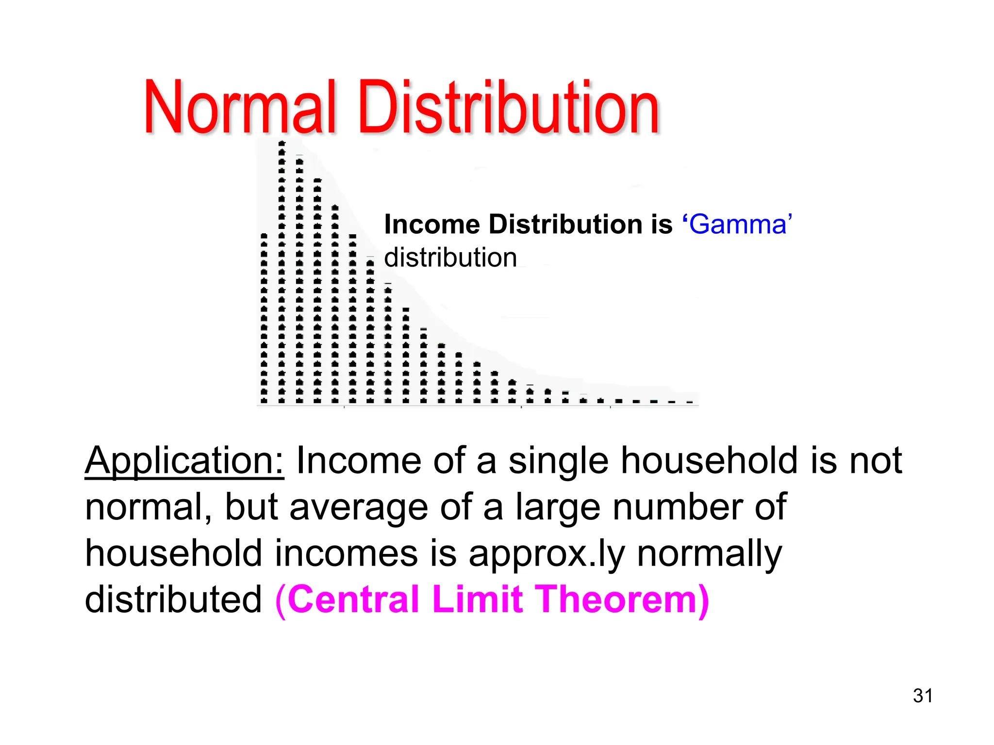
Normal Distribution
Application: Income of a single household is not
normal, but average of a large number of
household incomes is approx.ly normally
distributed (Central Limit Theorem)
Income Distribution is ‘Gamma’
distribution

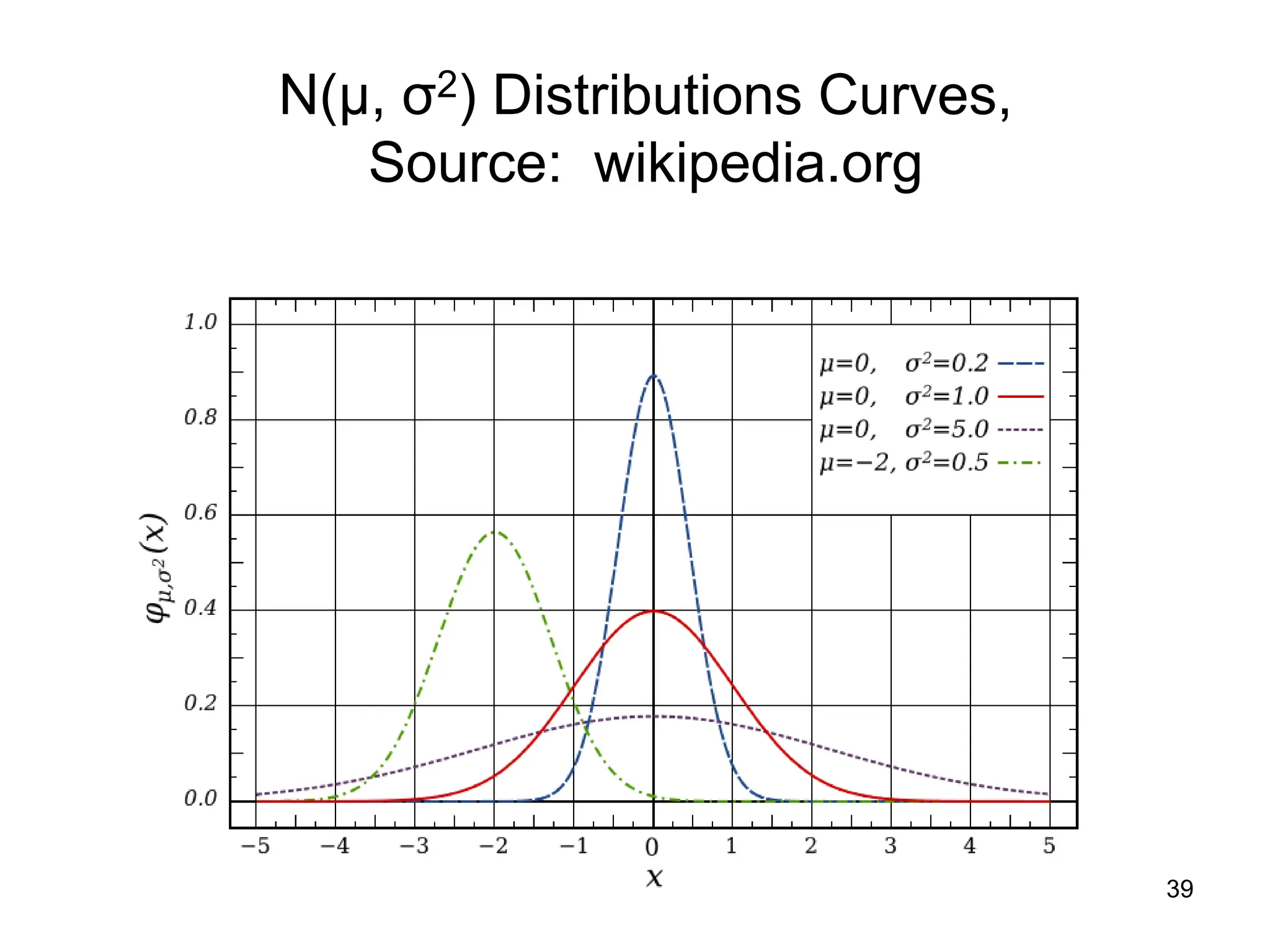
32. 32
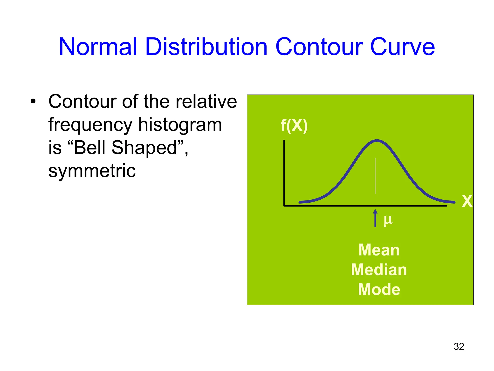
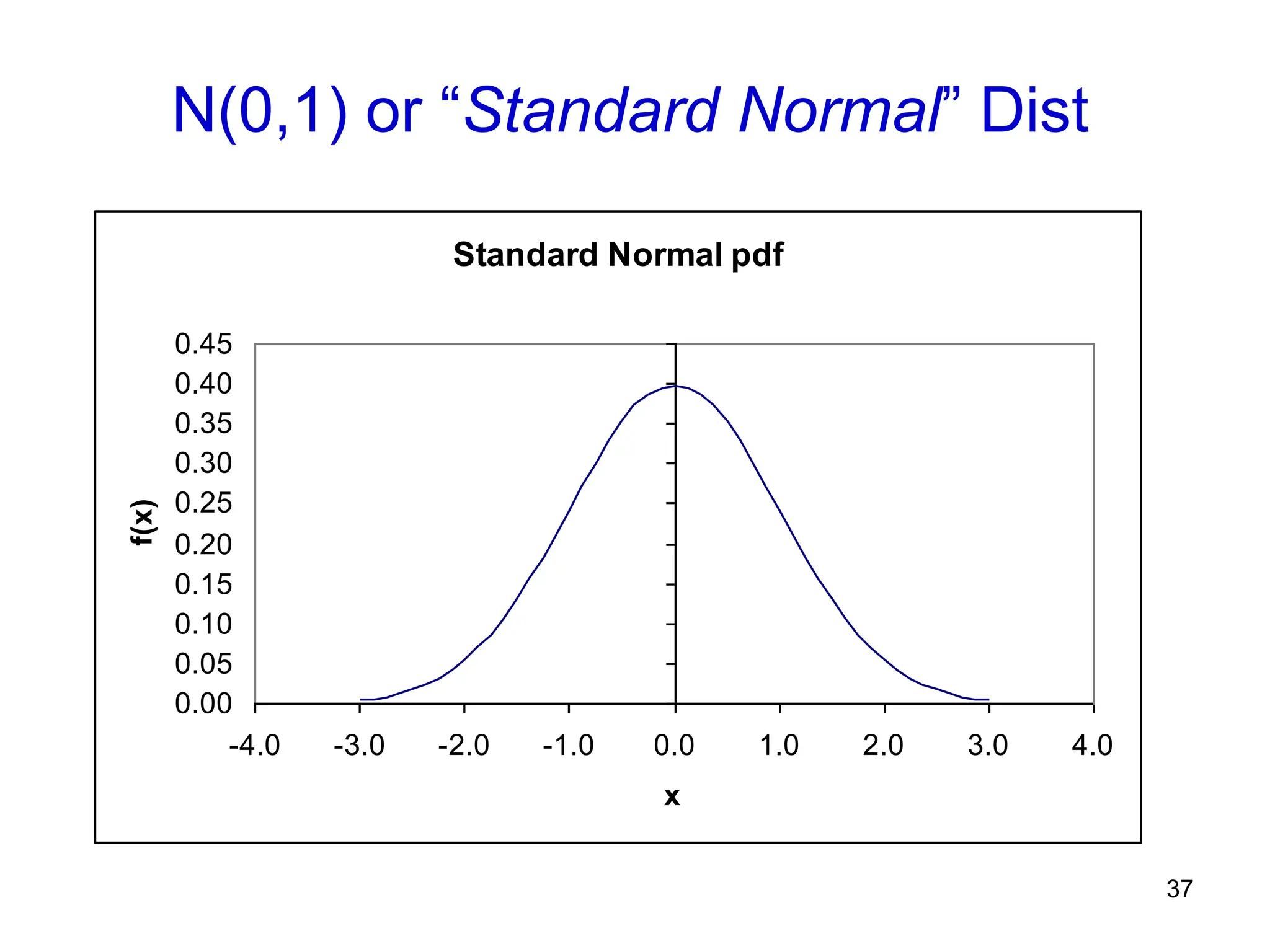
Normal Distribution Contour Curve
• Contour of the relative
frequency histogram
is “Bell Shaped”,
symmetric
Mean
Median
Mode
X
f(X)


33. 33
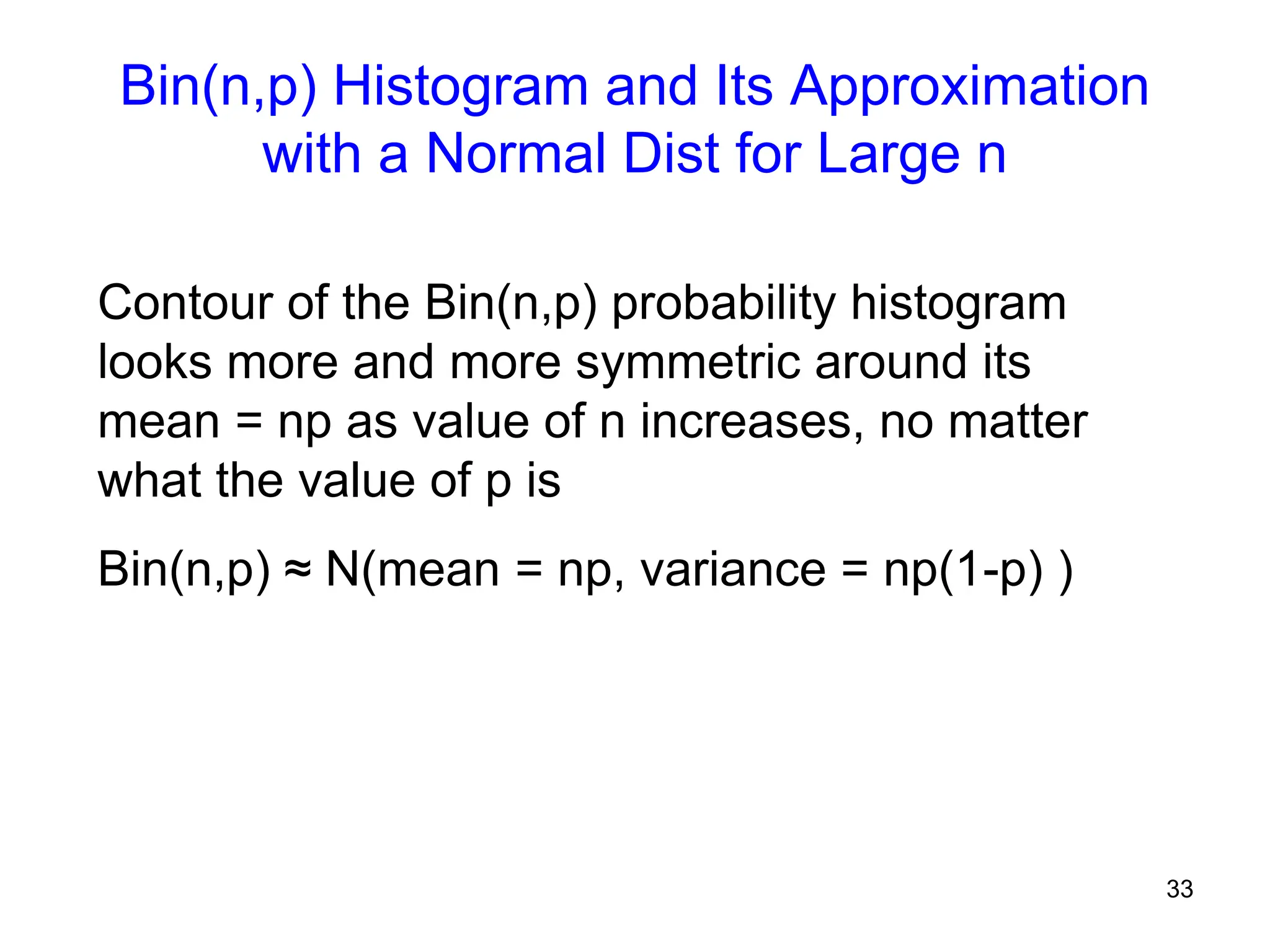
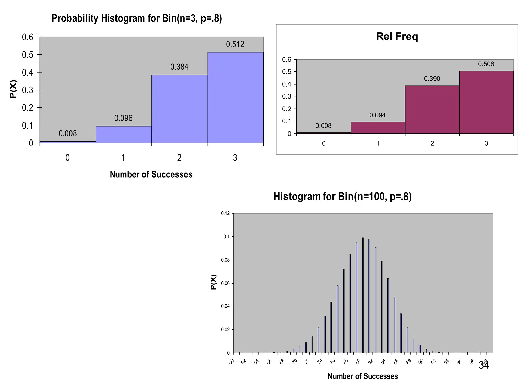
Bin(n,p) Histogram and Its Approximation
with a Normal Dist for Large n
Contour of the Bin(n,p) probability histogram
looks more and more symmetric around its
mean = np as value of n increases, no matter
what the value of p is
Bin(n,p) ≈ N(mean = np, variance = np(1-p) )

34. 34
Probability Histogram for Bin(n=3, p=.8)
0.008
0.096
0.384
0.512
0
0.1
0.2
0.3
0.4
0.5
0.6
0 1 2 3
Number of Successes
P(X)
Histogram for Bin(n=100, p=.8)
0
0.02
0.04
0.06
0.08
0.1
0.12
6
0
6
2
6
4
6
6
6
8
7
0
7
2
7
4
7
6
7
8
8
0
8
2
8
4
8
6
8
8
9
0
9
2
9
4
9
6
9
8
1
0
0
Number of Successes
P(X)
Rel Freq
0.008
0.094
0.390
0.508
0
0.1
0.2
0.3
0.4
0.5
0.6
0 1 2 3

35. 35
Nifty Prices 11 Jun 2007 - 11 Jun 2008
0.08
0.17
0.10
0.15
0.12 0.11
0.06
0.07
0.08
0.07
0
0.02
0.04
0.06
0.08
0.1
0.12
0.14
0.16
0.18
4
2
9
6
.
2
4
5
1
7
.
4
9
4
7
3
8
.
7
9
4
9
6
0
.
0
8
5
1
8
1
.
3
8
5
4
0
2
.
6
7
5
6
2
3
.
9
7
5
8
4
5
.
2
6
6
0
6
6
.
5
6
6
2
8
7
.
8
5

36. 36
NiftyReturns 11 June 2007- 11June 2008
0.00 0.00
0.03
0.06
0.15
0.41
0.25
0.06
0.02 0.02
0
0.05
0.1
0.15
0.2
0.25
0.3
0.35
0.4
0.45
-7.135 -5.57 -4.005 -2.44 -0.875 0.69 2.255 3.82 5.385 6.95

37. 37
Standard Normal pdf
0.00
0.05
0.10
0.15
0.20
0.25
0.30
0.35
0.40
0.45
-4.0 -3.0 -2.0 -1.0 0.0 1.0 2.0 3.0 4.0
x
f(x)
N(0,1) or “Standard Normal” Dist

38. 38
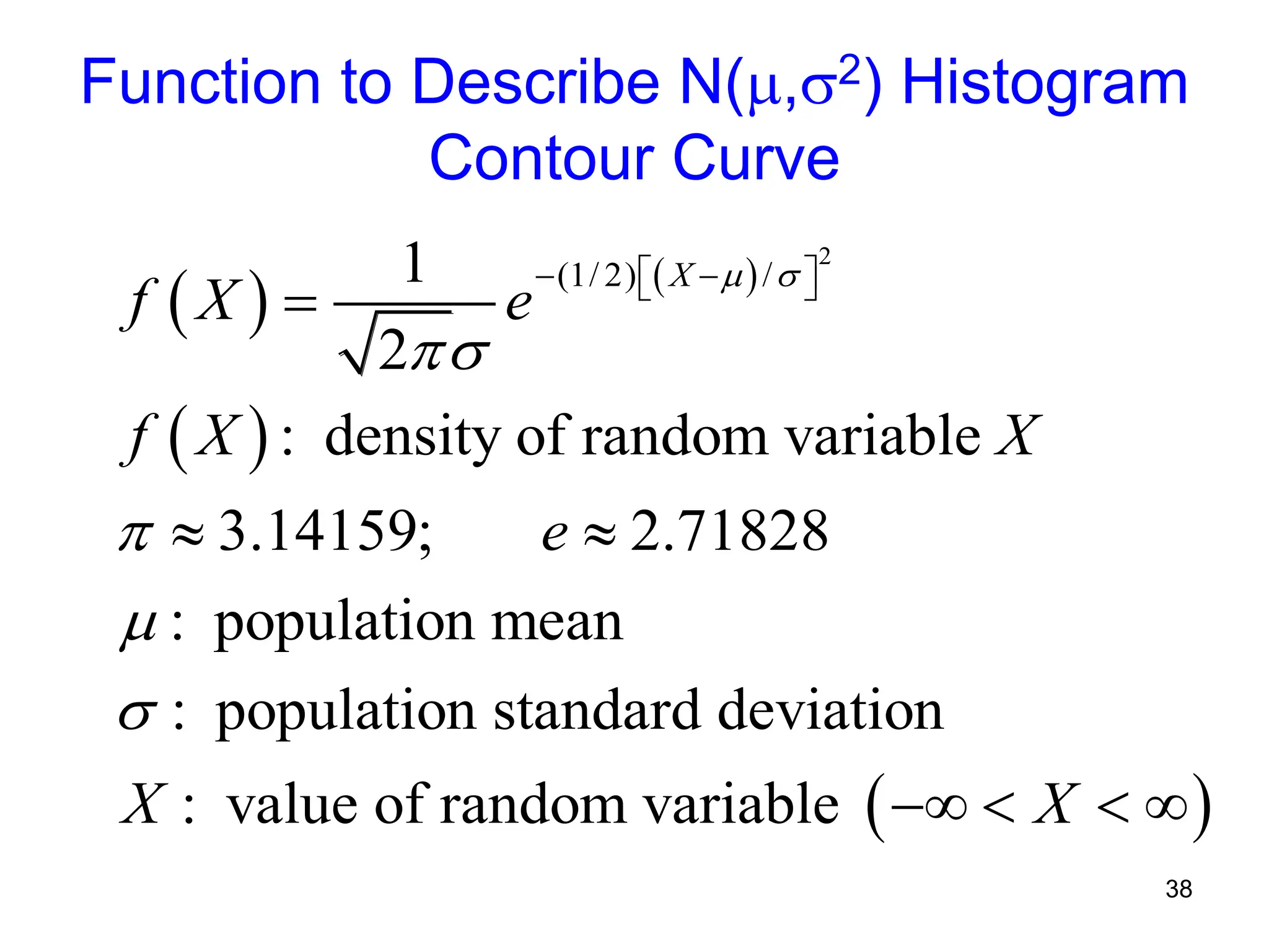
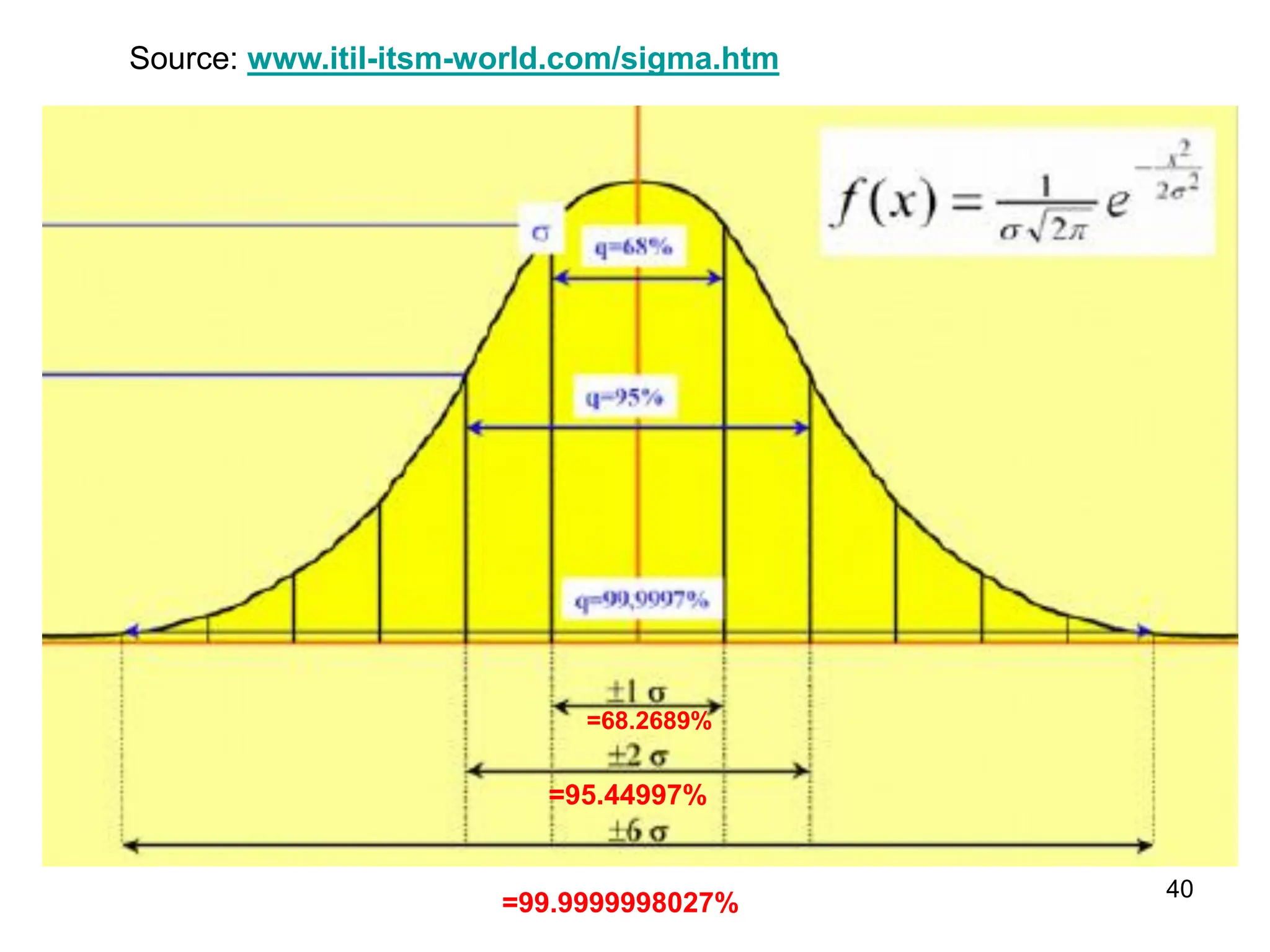
Function to Describe N(,2) Histogram
Contour Curve
   
 
 
2
(1/ 2) /
1
2
: density of random variable
3.14159; 2.71828
: population mean
: population standard deviation
: value of random variable
X
f X e
f X X
e
X X
 




 
 
 

 
   

39. 39
N(µ, σ2) Distributions Curves,
Source: wikipedia.org

40. 40
Source: www.itil-itsm-world.com/sigma.htm
=99.9999998027%
=95.44997%
=68.2689%

41. 41
Finding Probabilities
Probability is
the area under
the curve!
c d
X
f(X)
  ?
P c X d
  

42. 42
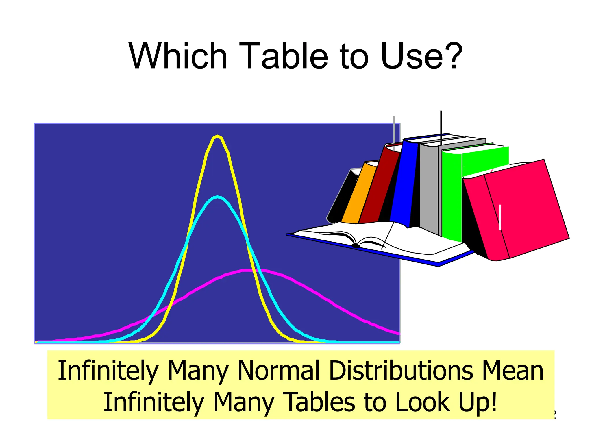
Which Table to Use?
Infinitely Many Normal Distributions Mean
Infinitely Many Tables to Look Up!

43. 43
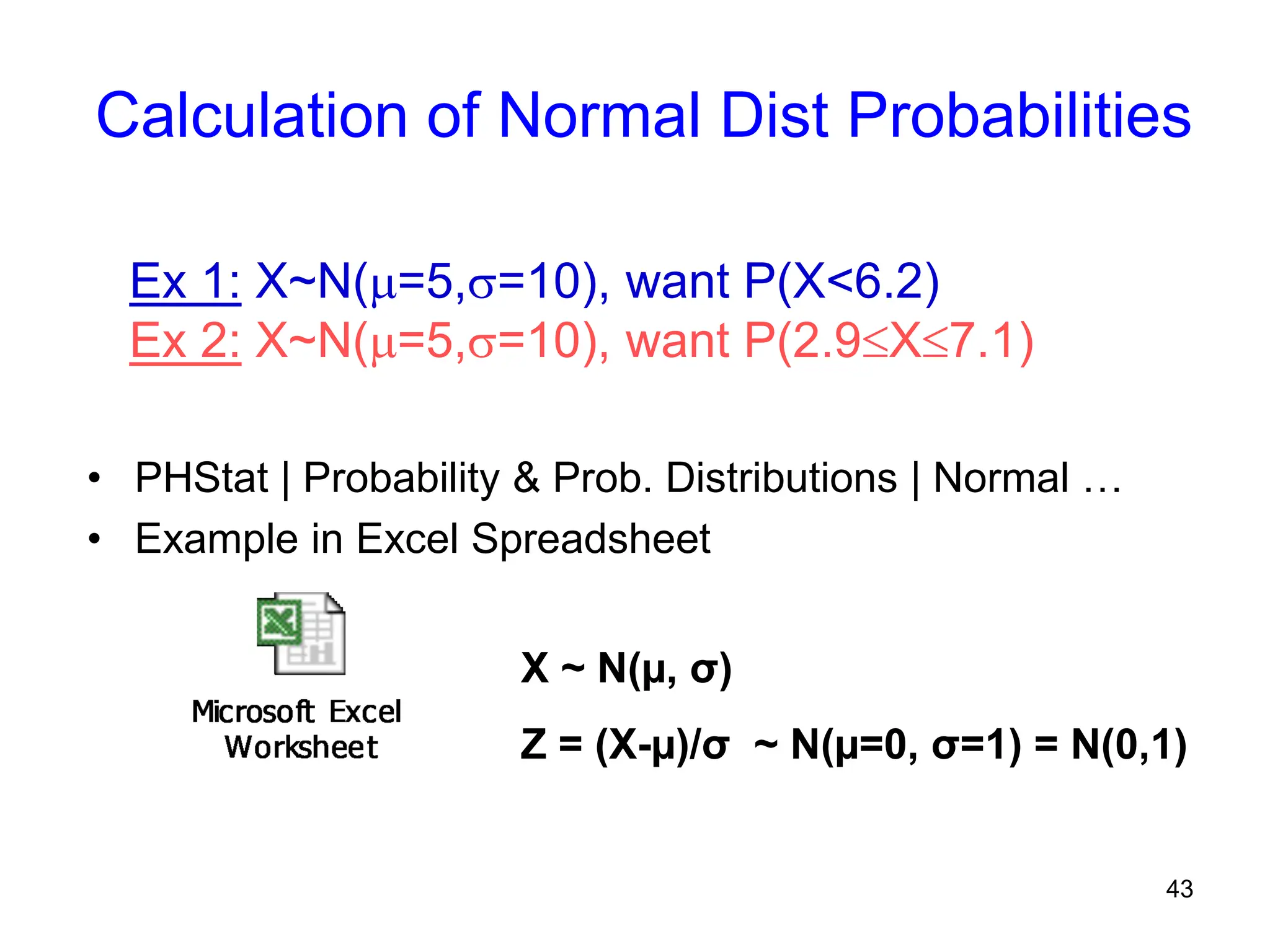
Calculation of Normal Dist Probabilities
• PHStat | Probability & Prob. Distributions | Normal …
• Example in Excel Spreadsheet
Ex 1: X~N(=5,=10), want P(X<6.2)
Ex 2: X~N(=5,=10), want P(2.9X7.1)
X ~ N(µ, σ)
Z = (X-µ)/σ ~ N(µ=0, σ=1) = N(0,1)

44. 44
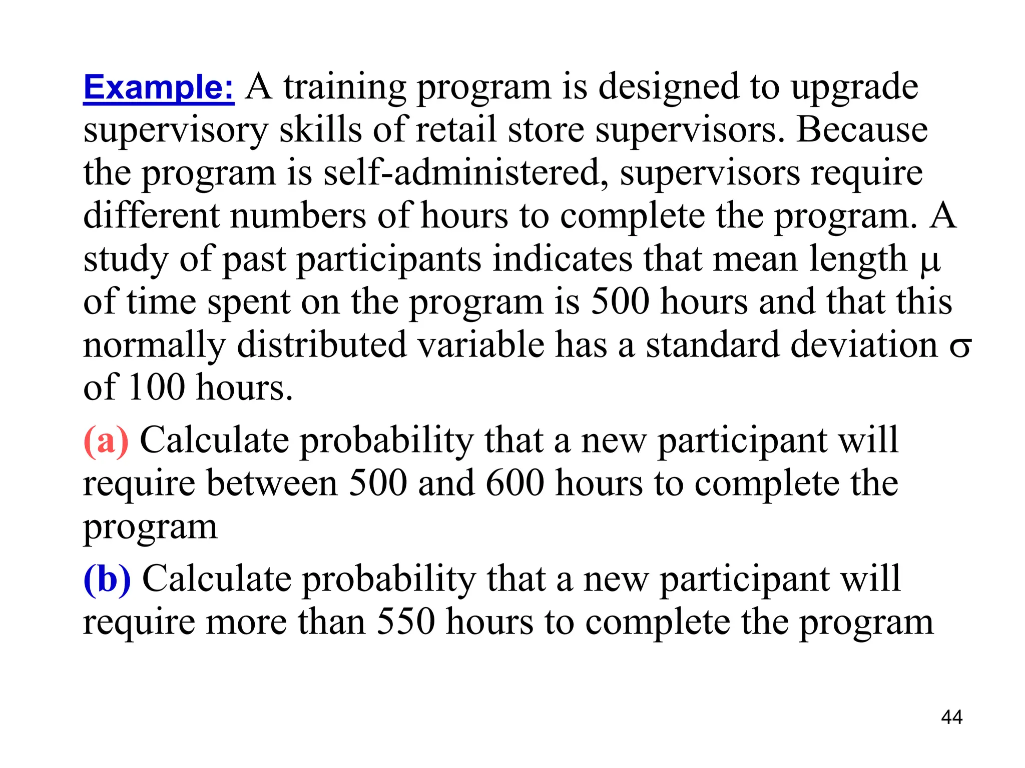
Example: A training program is designed to upgrade
supervisory skills of retail store supervisors. Because
the program is self-administered, supervisors require
different numbers of hours to complete the program. A
study of past participants indicates that mean length 
of time spent on the program is 500 hours and that this
normally distributed variable has a standard deviation 
of 100 hours.
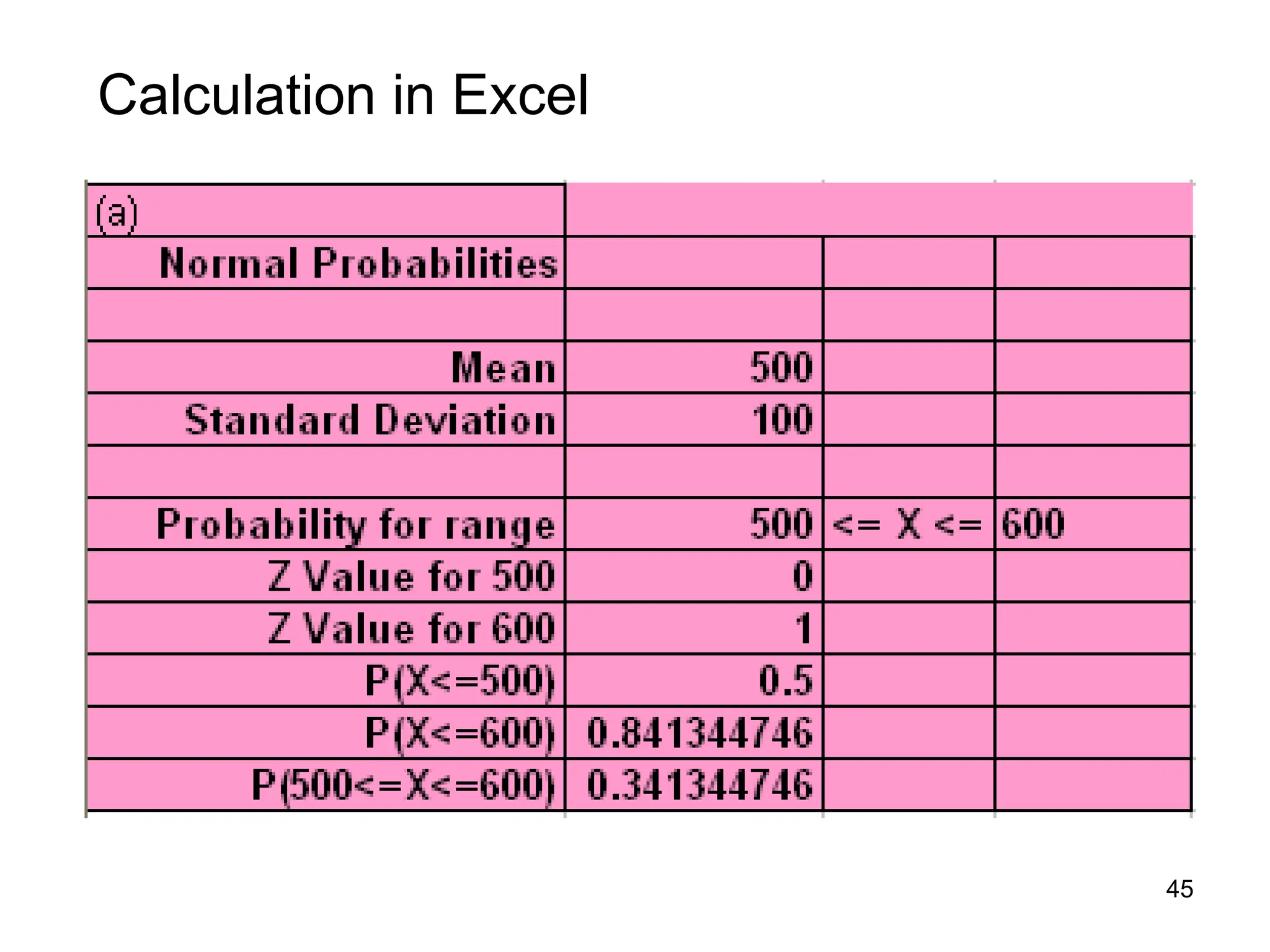
(a) Calculate probability that a new participant will
require between 500 and 600 hours to complete the
program
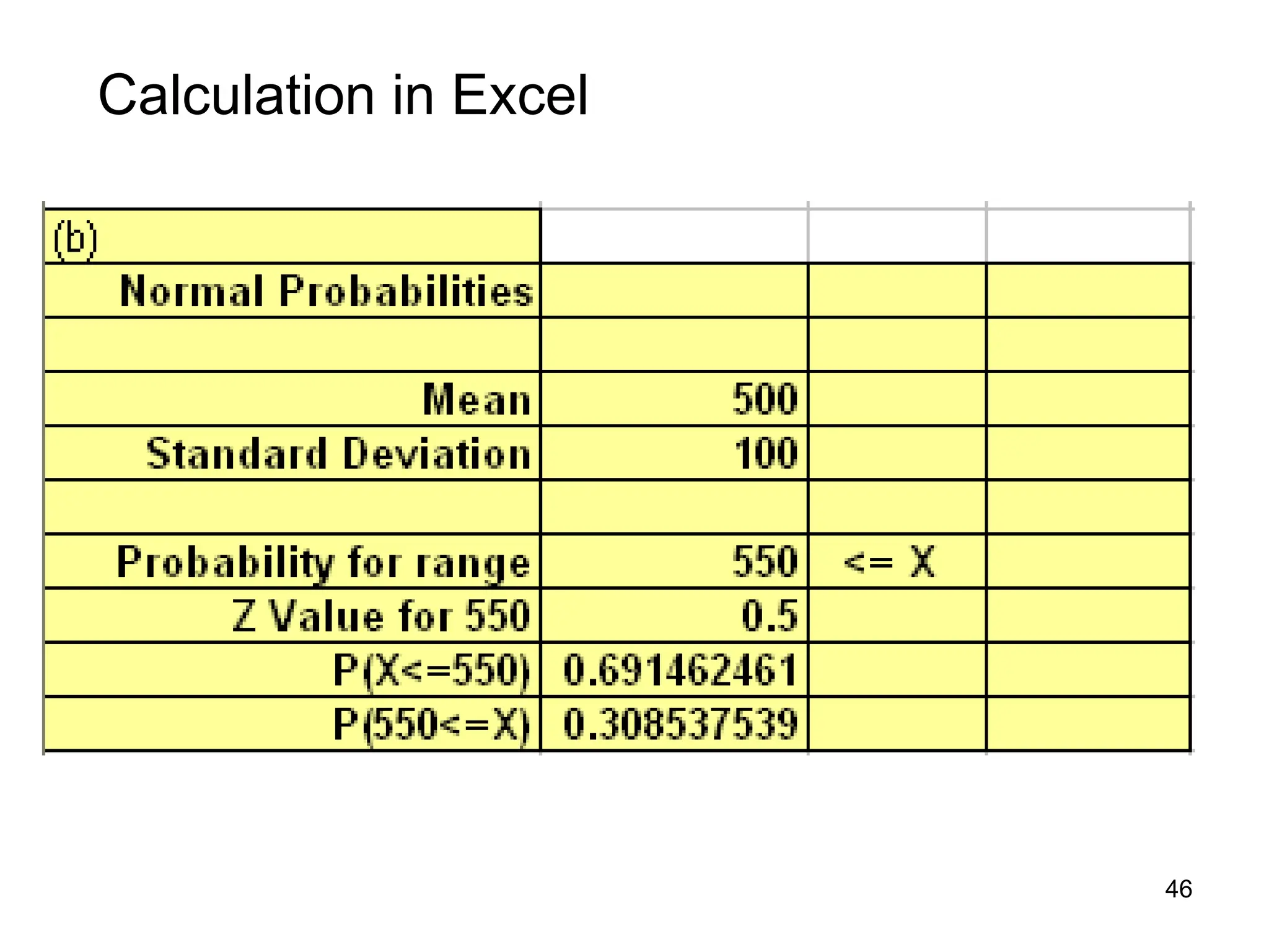
(b) Calculate probability that a new participant will
require more than 550 hours to complete the program

45. 45
Calculation in Excel

46. 46
Calculation in Excel

47. 47
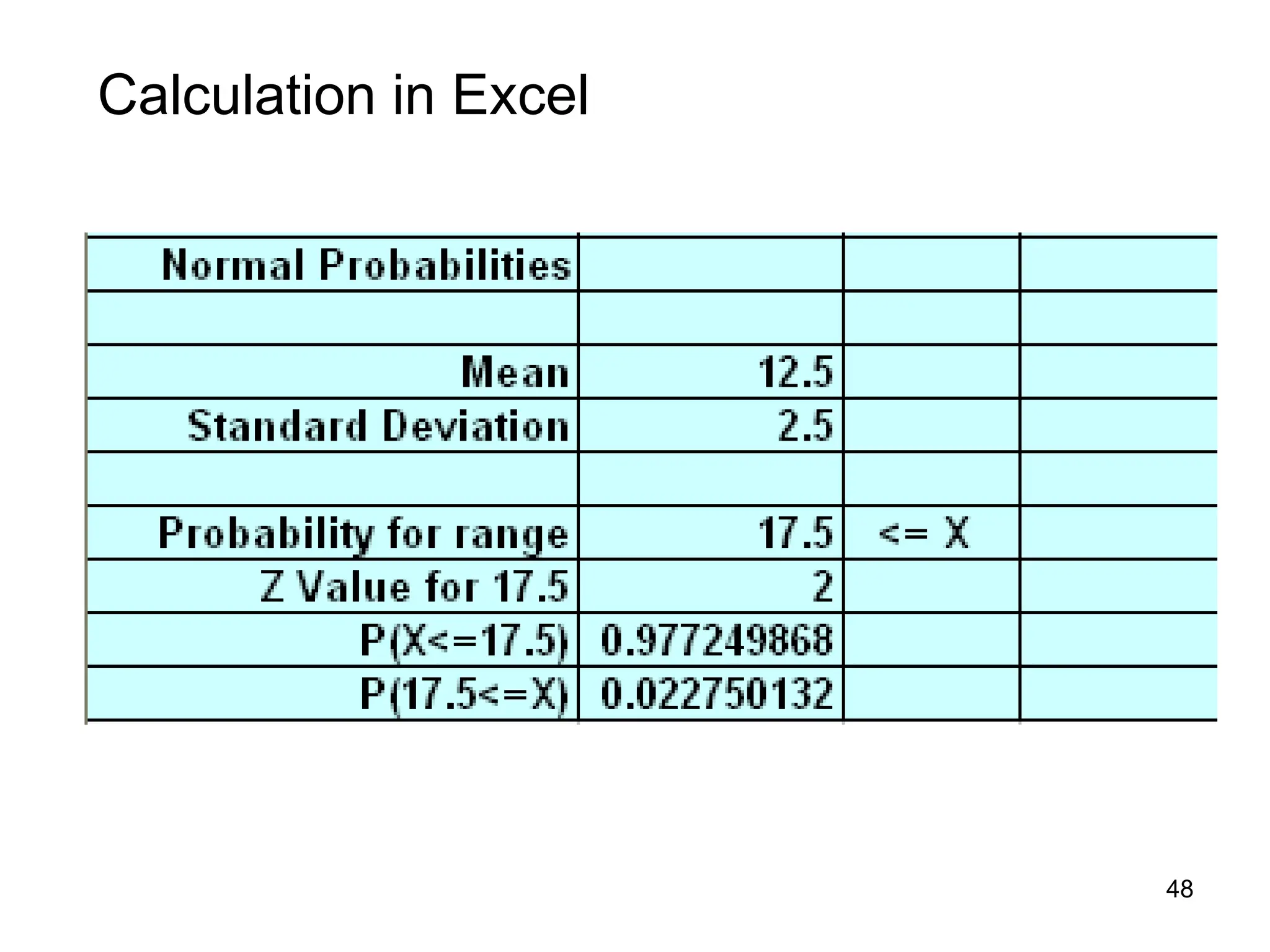
Example: According to global analyst Olivier
Lemaigre, the average price-to-earnings ratio (P/E) in
emerging markets is 12.5 with standard deviation of
2.5. Assume a normal distribution.
If a company in emerging markets is randomly selected,
what is the probability that its P/E is above 17.5 ?
(Suppose 17.5 =average for companies in the
developed world)

48. 48
Calculation in Excel

49. 49
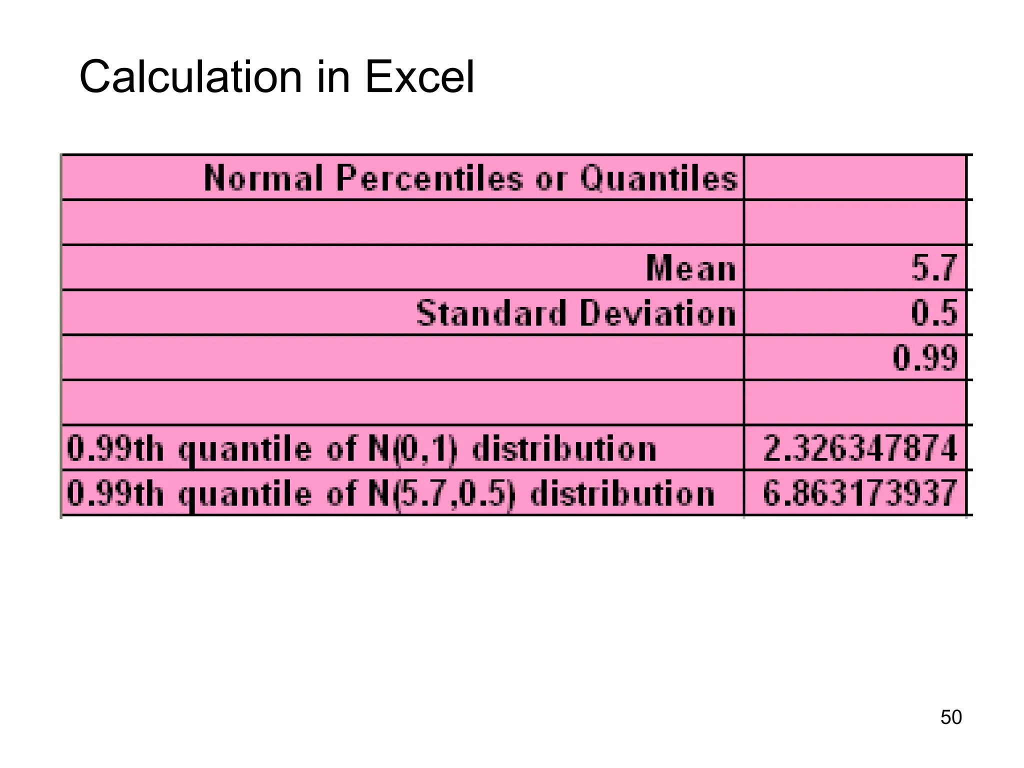
Example: The amount of fuel consumed by the engines
of a jetliner on a flight between two cities is a normally
distributed random variable X with mean =5.7 tons,
standard deviation =0.5 ton.
Carrying too much fuel is inefficient as it slows the
plane and if insufficient fuel is carried an emergency
landing may be necessary. The airline would like to
determine the amount of fuel to load so that there will
be 0.99 probability that the plane will arrive at its
destination.
Finding X Values for Known Probabilities

50. 50
Calculation in Excel

51. 51
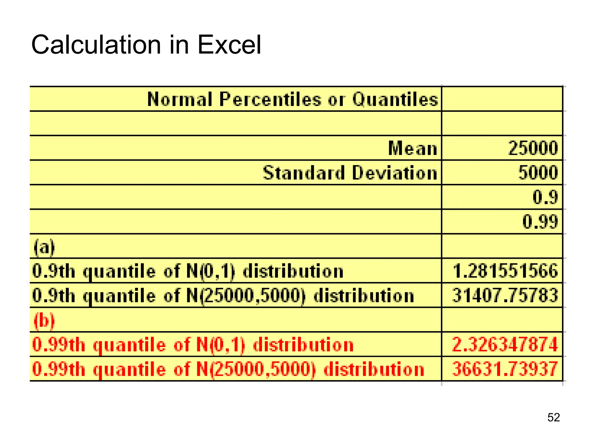
Example: A currency exchange office in Paris is open
at night when airport bank is closed and it makes most
of its business on returning US tourists who need to
change their remaining euros back to US dollars.
Experience shows that demand for dollars on any given
night during high season is approximately normally
distributed with mean $25,000 and st. dev. $5000.
If too much cash in dollars is carried there is a penalty
(i.e., interest on cash). If the office runs short of cash
during the night, it loses out on the potential profit.
How much cash in dollars should the office carry so
that demand on (a) 90%, (b) 99% of the nights will not
exceed this amount ?

52. 52
Calculation in Excel

53. 53
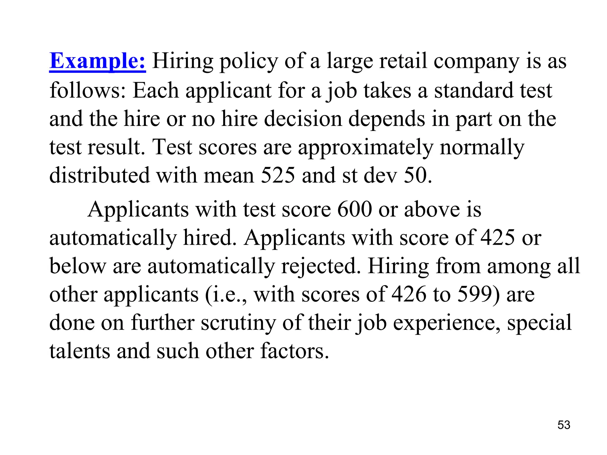
Example: Hiring policy of a large retail company is as
follows: Each applicant for a job takes a standard test
and the hire or no hire decision depends in part on the
test result. Test scores are approximately normally
distributed with mean 525 and st dev 50.
Applicants with test score 600 or above is
automatically hired. Applicants with score of 425 or
below are automatically rejected. Hiring from among all
other applicants (i.e., with scores of 426 to 599) are
done on further scrutiny of their job experience, special
talents and such other factors.

54. 54
Example (contd.)
• (a) Calculate the percentage of applicants who are
automatically rejected or accepted. [2.3% and
6.7%]
• (b) How to change the standards to automatically
reject 10% of all applicants and automatically
accept 15% of all applicants ? [Find the 10th and
85th percentiles: 461 (instead of 425) and 577 (instead
of 600)]
Use normal distribution and Excel