This document is the teacher's solutions manual for the Holt Physics textbook. It contains copyright information for Holt, Rinehart and Winston, the publisher, and details that the materials are not to be resold. The solutions are organized into two sections - the first section provides solutions to problems in the student edition textbook chapters, while the second section provides solutions to problems in the problem workbook. The manual contains solutions for all 22 chapters of the textbook and their respective appendices, covering the full range of high school physics content.


![Copyright
©
by
Holt,
Rinehart
and
Winston.
All
rights
reserved.
Section One—Student Edition Solutions I Ch. 1–3
I
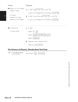
20. a. 756 g + 37.2 g + 0.83 g + 2.5 g = 796.53 g =
b.
3
3
.5
.2
6
m
3 s
= 0.898119562 m/s =
c. 5.67 mm × p = 17.81283035 mm =
d. 27.54 s − 3.8 s = 23.74 s =
21. 93.46 cm, 135.3 cm 93.46 cm + 135.3 cm = 228.76 cm =
22. l = 38.44 m w = 19.5 m 38.44 m + 38.44 m + 19.5 m + 19.5 m = 115.88 m =
26. s = (a + b + c) ÷ 2 r =
r, a, b, c, and s all have units of L.
length =
=
=
(l
en
gt
h
)2
= length
Thus, the equation is dimensionally consistent.
27. T = 2p
Substitute the proper dimensions into the equation.
time =
=
(t
im
e)
2
= time
Thus, the dimensions are consistent.
28. (m/s)2
≠ m/s2
× s
m2
/s2
≠ m/s
The dimensions are not consistent.
29. Estimate one breath every 5 s.
70 years ×
36
1
5
y
d
ea
a
r
ys
×
1
24
da
h
y
×
36
1
0
h
0 s
×
1 b
5
re
s
ath
=
30. Estimate one heart beat per second.
1 day ×
1
24
da
h
y
×
36
1
0
h
0 s
×
1 b
s
eat
=
31. Ages will vary.
17 years ×
36
1
5
y
d
ea
a
r
ys
×
1
24
da
h
y
×
36
1
0
h
0 s
=
32. Estimate a tire’s radius to be 0.3 m.
50 000 mi ×
1.6
1
0
m
9 k
i
m
×
1
1
0
k
3
m
m
×
2 p
1
(0
r
.
e
3
v
m)
= 4 × 10⁷
rev
5.4 × 10⁸
s
9 × 10⁴
beats
4 × 10⁸
breaths
length
[length/(time)2
]
L
ag
(length)3
length
length × length × length
length
(s − a)(s − b)(s − c)
s
115.9 m
228.8 cm
23.7 s
17.8 mm
0.90 m/s
797 g
Givens Solutions](https://image.slidesharecdn.com/physicssolutions-230306125240-7bc050a7/85/physics-solutions-pdf-11-320.jpg)

![Holt Physics Solution Manual
I Ch. 2–2
Copyright
©
by
Holt,
Rinehart
and
Winston.
All
rights
reserved.
I
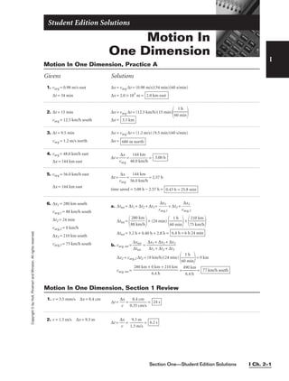
3. ∆x1 = 50.0 m south
∆t1 = 20.0 s
∆x2 = 50.0 m north
∆t2 = 22.0 s
4. v1 = 0.90 m/s
v2 = 1.90 m/s
∆x = 780 m
∆t1 − ∆t2 =
(5.50 min)(60 s/min) =
3.30 × 10²
s
a. vavg,1 =
∆
∆
x
t1
1
=
5
2
0
0
.
.
0
0
m
s
=
b. vavg,2 =
∆
∆
x
t2
2
=
5
2
0
2
.
.
0
0
m
s
=
∆xtot = ∆x1 + ∆x2 = (−50.0 m) + (50.0 m) = 0.0 m
∆ttot = ∆t1 + ∆t2 = 20.0 s + 22.0 s = 42.0 s
vavg =
∆
∆
x
tt
t
o
o
t
t
=
4
0
2
.0
.0
m
s
= 0.0 m/s
2.27 m/s north
2.50 m/s south
a. ∆t1 =
∆
v1
x
=
0
7
.9
8
0
0
m
m
/s
= 870 s
∆t2 =
∆
v2
x
=
1
7
.9
8
0
0
m
m
/s
= 410 s
∆t1 − ∆t2 = 870 s − 410 s =
b. ∆x1 = v1∆t1
∆x2 = v2∆t2
∆x1 = ∆x2
v1∆t1 = v2∆t2
v1[∆t2 + (3.30 × 10²
s)] = v2∆t2
v1∆t2 + v1(3.30 × 10²
s) = v2∆t2
∆t2 (v1 − v2) = −v1(3.30 × 10²
s)
∆t2 =
−v1(3
v
.3
1
0
−
×
v2
102
s)
= =
∆t2 = 3.0 × 10²
s
∆t1 = ∆t2 + (3.30 × 10²
s) = (3.0 × 10²
s) + (3.30 × 10²
s) = 630 s
∆x1 = v1∆t1 = (0.90 m/s)(630 s) =
∆x2 = v2∆t2 = (1.90 m/s)(3.0 × 102
s) = 570 m
570 m
−(0.90 m/s)(3.30 × 102
s)
−1.00 m/s
−(0.90 m/s)(3.30 × 102
s)
0.90 m/s − 1.90 m/s
460 s
Givens Solutions
1. aavg = − 4.1 m/s2
∆t =
a
∆
a
v
vg
= = =
–
–
4
9
.
.
1
0
m
m
/
/
s
s
2
=
vi = 9.0 m/s
vf = 0.0 m/s
2. aavg = 2.5 m/s2
∆t =
a
∆
a
v
vg
= =
12.0 m
2.5
/s
m
–
/
7
s
.
2
0 m/s
=
2
5
.
.
5
0
m
m
/
/
s
s
2
=
vi = 7.0 m/s
vf = 12.0 m/s
3. aavg = −1.2 m/s2
∆t =
v
a
f
a
−
vg
vi
= =
−
−
1
6
.
.
2
5
m
m
/
/
s
s
2
=
vi = 6.5 m/s
vf = 0.0 m/s
5.4 s
0.0 m/s − 6.5 m/s
− 1.2 m/s2
2.0 s
vf – vi
aavg
2.2 s
0.0 m/s – 9.0 m/s
– 4.1 m/s2
vf – vi
aavg
Motion In One Dimension, Practice B](https://image.slidesharecdn.com/physicssolutions-230306125240-7bc050a7/85/physics-solutions-pdf-16-320.jpg)


![Holt Physics Solution Manual
I Ch. 2–6
Copyright
©
by
Holt,
Rinehart
and
Winston.
All
rights
reserved.
I
3. vi = +8.0 m/s
a = −9.81 m/s2
∆y = 0 m
4. vi = +6.0 m/s
vf = +1.1 m/s2
a = −9.81 m/s2
∆y = =
∆y = =
−
−
1
3
9
5
.6
m
m
2
/
/
s
s
2
2
= +1.8 m
1.2 m2
/s2
− 36 m2
/s2
−19.6 m/s2
(1.1 m/s)2
− (6.0 m/s)2
(2)(−9.81 m/s2
)
vf
2
− vi
2
2a
a. vf =
v i
2
+ 2
ay
=
(8
.0
m
/s
)2
+
(
2)
(−
9.
81
m
/s
2)
(0
m
)
vf =
64 m2
/
s2
= ±8.0 m/s =
b. ∆t =
vf
a
− vi
=
−8.0
−
m
9.
/
8
s
1
−
m
8
/
.
s
0
2
m/s
=
−
−
9
1
.
6
8
.
1
0
m
m
/
/
s
s
2
= 1.63 s
−8.0 m/s
Givens Solutions
2. vi = 0 m/s ∆y = vi∆t +
1
2
a∆t2
= (0 m/s)(1.5 s) +
1
2
(−9.81 m/s2
)(1.5 s)2
∆t = 1.5 s ∆y = 0 m + (−11 m) = −11 m
a = −9.81 m/s2
the distance to the water’s surface = 11 m
Motion In One Dimension, Section 3 Review
7. ∆t = 0.530 h ∆x = vavg ∆t = (19.0 km/h)(0.530 h) =
vavg = 19.0 km/h east
8. ∆t = 2.00 h, 9.00 min, 21.0 s ∆x = vavg ∆t = (5.436 m/s) [(2.00 h)(3600 s/h) + (9.00 min)(60 s/min) + 21.0 s]
vavg = 5.436 m/s ∆x =(5.436 m/s)(7200 s + 540 s + 21.0 s) = (5.436 m/s)(7760 s)
∆x =4.22 × 10⁴
m =
9. ∆t = 5.00 s a. ∆xA =
distance between b. ∆xB = 70.0 m + 70.0 m =
poles = 70.0 m
c. vavg,A =
∆
∆
x
t
A
=
7
5
0
.
.
0
0
s
m
=
d. vavg,B =
∆
∆
x
t
B
=
1
5
4
.
0
0
m
s
= +28 m/s
+14 m/s
+140.0 m
+70.0 m
4.22 × 101
km
10.1 km east
Motion In One Dimension, Chapter Review](https://image.slidesharecdn.com/physicssolutions-230306125240-7bc050a7/85/physics-solutions-pdf-20-320.jpg)


![Section One—Student Edition Solutions I Ch. 2–13
Copyright
©
by
Holt,
Rinehart
and
Winston.
All
rights
reserved.
I
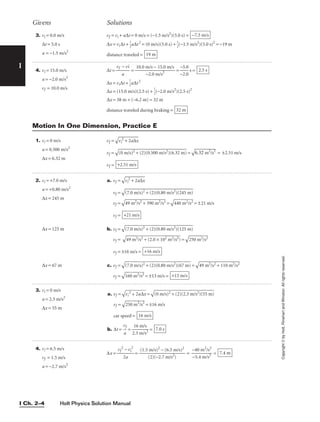
42. vs = 30.0 m/s a. ∆xs = ∆xp
vi,p = 0 m/s ∆xs = vs∆t
ap = 2.44 m/s2
Because vi,p = 0 m/s,
∆xp =
1
2
ap∆t2
vs∆t =
1
2
ap∆t2
∆t =
2
a
v
p
s
=
(2
2
)(
.4
3
4
0.
m
0 m
/s2
/s)
=
b. ∆xs = vs∆t = (30.0 m/s)(24.6 s) =
or ∆xp =
1
2
ap∆t2
=
1
2
(2.44 m/s2
)(24.6 s)2
= 738 m
738 m
24.6 s
43. For ∆t1:
vi = 0 m/s
a = +13.0 m/s2
vf = v
For ∆t2:
a = 0 m/s2
v = constant velocity
∆xtot = +5.30 × 10³
m
∆ttot = ∆t1 + ∆t2 = 90.0 s
When vi = 0 m/s,
∆x1 =
1
2
a∆t1
2
∆t2 = 90.0 s − ∆t1
∆x2 = v∆t2 = v(90.0 s − ∆t1)
∆xtot = ∆x1 + ∆x2 =
1
2
a∆t1
2
+ v(90.0 s − ∆t1)
v = vf during the first time interval = a∆t1
∆xtot =
1
2
a∆t1
2
+ a∆t1(90.0 s − ∆t1) =
1
2
a∆t1
2
+ (90.0 s)a∆t1 − a∆t1
2
∆xtot = −
1
2
a∆t1
2
+ (90.0 s)a∆t1
1
2
a∆t1
2
− (90.0 s)a∆t1 + ∆xtot = 0
Using the quadratic equation,
∆t1 =
∆t1 =
(90.0s)(13.0m/s2
) ±
[−(90.0
s)(13.
0 m/s2
)]2
−2(
13.0 m
/s)(5.3
0 × 103
m)
13.0 m/s2
(90.0 s)(a) ±[−(90.0
s)(a)]
2
− 4
1
2
a
(∆xtot)
2
1
2
a
∆t1 =
∆t1 = = =
13
6
.
0
0
m
m
/
/
s
s2
=
∆t2 = ∆ttot − ∆t1 = 90.0 s − 5 s =
v = a∆t1 = (13.0 m/s2
)(5 s) = +60 m/s
85 s
5 s
1170 m/s ± 1110 m/s
13.0 m/s2
1170 m/s ±
1.23 ×
106 m2
/s2
13.0 m/s2
1170 m/s ±
(1.37 ×
106 m
2/s2) −
(1.38
× 105 m
2/s2)
13.0 m/s2](https://image.slidesharecdn.com/physicssolutions-230306125240-7bc050a7/85/physics-solutions-pdf-27-320.jpg)


![Holt Physics Solution Manual
I Ch. 2–16
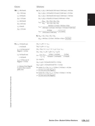
49. a1 = +5.9 m/s2
a2 = +3.6 m/s2
∆t1 = ∆t2 − 1.0 s
Because both cars are initially at rest,
a. ∆x1 =
1
2
a1∆t1
2
∆x2 =
1
2
a2∆t2
2
∆x1 = ∆x2
1
2
a1∆t1
2
=
1
2
a2∆t2
2
a1(∆t2 − 1.0 s)2
= a2∆t2
2
a1[∆t2
2
− (2.0 s)(∆t2) + 1.0 s2
] = a2∆t2
2
(a1)(∆t2)2
− a1(2.0 s)∆t2 + a1(1.0 s2
) = a2∆t2
2
(a1 − a2)∆t2
2
− a1(2.0 s)∆t2 + a1(1.0 s2
) = 0
Using the quadratic equation,
∆t2 =
a1 − a2 = 5.9 m/s2
− 3.6 m/s2
= 2.3 m/s2
∆t2 =
∆t2 = =
∆t2 =
1
(
2
2)
m
(2
/s
.3
±
m
9
/
m
s2)
/s
=
(2)(
2
2
1
.3
m
m
/s
/s2)
=
∆t1 = ∆t2 − 1.0 s = 4.6 s − 1.0 s =
b. ∆x1 =
1
2
a1∆t1
2
=
1
2
(5.9 m/s2
)(3.6 s)2
= 38 m
or ∆x2 =
1
2
a2∆t2
2
=
1
2
(3.6 m/s2
)(4.6 s)2
= 38 m
distance both cars travel =
c. v1 = a1∆t1 = (5.9 m/s2
)(3.6 s) =
v2 = a2∆t2 = (3.6 m/s2
)(4.6 s) = +17 m/s
+21 m/s
38 m
3.6 s
4.6 s
12 m/s ±
90 m2/
s2
(2)(2.3 m/s2)
12 m/s ±
140 m2
/s2 − 5
4 m2/s
2
(2)(2.3 m/s2)
(5.9 m/s2
)(2.0 s) ±
[−(5.9
m/s2)(
2.0 s)]
2
− (4)
(2.3 m
/s2)(5.
9 m/s2
)(1.0 s
2)
(2)(2.3 m/s2)
(a1)(2.0 s) ±
[−a1(2
.0 s)]2
− 4(a1
− a2)a1
(1.0 s2
)
2(a1 − a2)
I
Givens Solutions
Copyright
©
by
Holt,
Rinehart
and
Winston.
All
rights
reserved.
50. vi,1 = +25 m/s
vi,2 = +35 m/s
∆x2 = ∆x1 + 45 m
a1 = −2.0 m/s2
vf,1 = 0 m/s
vf,2 = 0 m/s
a. ∆t1 =
vf,1
a
−
1
vi,1
=
0 m
−
/
2
s
.0
−
m
25
/s
m
2
/s
=
b. ∆x1 =
1
2
(vi,1 + vf,1)∆t1 =
1
2
(25 m/s + 0 m/s)(13 s) = +163 m
∆x2 = ∆x1 + 45 m = 163 m + 45 m = +208 m
a2 =
vf,2
2
2
∆
−
x
v
2
i,2
2
= =
c. ∆t2 =
vf,2
a
−
2
vi,2
=
0 m
−
/
2
s
.9
−
m
35
/s
m
2
/s
= 12 s
−2.9 m/s2
(0 m/s)2
− (35 m/s)2
(2)(208 m)
13 s](https://image.slidesharecdn.com/physicssolutions-230306125240-7bc050a7/85/physics-solutions-pdf-30-320.jpg)

![Copyright
©
by
Holt,
Rinehart
and
Winston.
All
rights
reserved.
Section One—Student Edition Solutions I Ch. 3–1
Two-Dimensional Motion
and Vectors
Student Edition Solutions
I
2. ∆x1 = 85 m
d2 = 45 m
q2 = 30.0°
3. vy, 1 = 2.50 × 10²
km/h
v2 = 75 km/h
q2 = −45°
4. vy,1 =
2.50 × 1
2
02
km/h
= 125 km/h
vx,2 = 53 km/h
vy,2 = −53 km/h
Students should use graphical techniques. Their answers can be checked using the
techniques presented in Section 2. Answers may vary.
∆x2 = d2(cos q2) = (45 m)(cos 30.0°) = 39 m
∆y2 = d2(sin q2) = (45 m)(sin 30.0°) = 22 m
∆xtot = ∆x1 + ∆x2 = 85 m + 39 m = 124 m
∆ytot = ∆y2 = 22 m
d =
(∆
xt
ot
)2
+
(
∆
yt
ot
)2
=
(1
24
m
)2
+
(
22
m
)2
d =
15
4
00
m
2
+
4
80
m
2
=
15
9
00
m
2
=
q = tan−1
∆
∆
x
yt
t
o
o
t
t
= tan−1
1
2
2
2
4
m
m
= (1.0 × 101
)° above the horizontal
126 m
Students should use graphical techniques.
vx,2 = v2(cos q2) = (75 km/h)[cos (−45°)] = 53 km/h
vy,2 = v2(sin q2) = (75 km/h)[sin (−45°)] = −53 km/h
vy,tot = vy,1 + vy,2 = 2.50 × 10²
km/h − 53 km/h = 197 km/h
vx,tot = vs,2 = 53 km/h
v =
(v
x,
to
t)
2
+
(
vy
,to
t)
2
=
(5
3
km
/h
)2
+
(1
97
k
m
/h
)2
v =
28
00
k
m
2
/
h
2
+
3
8
80
0
km
2
/
h
2
=
41
6
00
k
m
2
/
h
2
=
q = tan−1
v
v
x
y,
,
t
t
o
o
t
t
= tan−1
2
5
0
3
4
k
k
m
m
/
/
h
h
= 75° north of east
204 km/h
Students should use graphical techniques.
vy,dr = vy,1 + vy,2 = 125 km/h − 53 km/h = 72 km/h
vx,dr = vx,2 = 53 km/h
v =
(v
x,
dr
)2
=
v
y,d
r)
2
=
(5
3
km
/h
)2
+
(7
(7
2
km
/h
)2
v =
28
00
k
m
2
/
h
2
+
5
20
0
km
2
/
h
2
=
8.
0
1
03
k
m
2
/
h
2
=
q = tan−1
v
v
x
y,
,
d
d
r
r
= tan−1
7
5
2
3
k
k
m
m
/
/
h
h
= 54° north of east
89 km/h
Two-Dimensional Motion and Vectors, Section 1 Review
Givens Solutions](https://image.slidesharecdn.com/physicssolutions-230306125240-7bc050a7/85/physics-solutions-pdf-33-320.jpg)
![Givens Solutions
Holt Physics Solution Manual
I Ch. 3–6
I
Copyright
©
by
Holt,
Rinehart
and
Winston.
All
rights
reserved.
4. ∆x = 2.00 m
∆y = 0.55 m
q = 32.0°
ay = −g = −9.81 m/s2
∆x = vi(cos q)∆t
∆t =
vi(c
∆
o
x
s q)
∆y = vi(sin q)∆t +
1
2
ay∆t2
= vi(sin q)
vi(c
∆
o
x
s q)
+
1
2
ay
vi(c
∆
o
x
s q)
2
∆y = ∆x(tan q) +
2vi
2
a
(
y
c
∆
o
x
s
2
q)2
∆x(tan q) − ∆y =
2vi
−
2
a
(c
y∆
os
x2
q)2
2vi
2
(cos q)2
=
∆x(t
−
a
a
n
y∆
q)
x2
− ∆y
vi =
vi =
vi = = = 6.2 m/s
(9.81 m/s2
)(2.00 m)2
(2)(cos 32.0°)2
(0.70 m)
(9.81 m/s2
)(2.00 m)2
(2)(cos 32.0°)2
(1.25 − 0.55 m)
(9.81 m/s2
)(2.00 m)2
(2)(cos 32.0°)2
[(2.00 m)(tan 32.0°) − 0.55 m]
−ay∆x2
2(cos q)2
[∆x(tan q) − ∆y]
2. ∆y = −125 m
vx = 90.0 m/s
ay = −g = −9.81 m/s2
∆y =
1
2
ay∆t2
∆t =
2
a
∆
y
y
=
(
−
2
)
9
(
.
−
8
1
1
2
m
5
/
m
s
2
)
=
∆x = vx∆t = (90.0 m/s)(5.05 s) = 454 m
5.05 s
Two-Dimensional Motion and Vectors, Section 3 Review
3. vx = 30.0 m/s
∆y = −200.0 m
ay = −g = −9.81 m/s2
vx = 30.0 m/s
∆y = −200.0 m
ay = −g = −9.81 m/s2
∆x = 192 m
a. ∆y =
1
2
ay∆t2
∆t =
2
a
∆
y
y
∆x = vx∆t = vx
2
a
∆
y
y
= (30.0 m/s)
(2
−
)(
9
−
.8
2
1
00
m
.0
/s
m
2
)
=
b. vy =
vy,i
2
+ 2
ay∆y
=
(0 m/s
)2
+ (2
)(−9.81
m/s2
)(
−200.0
m)
= ±62.6 m/s = −62.6 m/s
vtot =
vx
2
+ v
y
2
=
(30.0 m
/s)2
+ (
−62.6 m
/s)2
=
9.00 ×
102
m2
/s2
+ 3
.92 × 1
03
m2
/
s2
vtot =
4820 m
2
/s2
=
q = tan−1
v
v
x
y
= tan−1
−
3
6
0
2
.0
.6
m
m
/
/
s
s
= −64.4°
q = 64.4° below the horizontal
69.4 m/s
192 m](https://image.slidesharecdn.com/physicssolutions-230306125240-7bc050a7/85/physics-solutions-pdf-38-320.jpg)


![Copyright
©
by
Holt,
Rinehart
and
Winston.
All
rights
reserved.
22. ∆y1 = −10.0 yards ∆ytot = ∆y1 + ∆y2 = −10.0 yards + 50.0 yards = 40.0 yards
∆x = 15.0 yards ∆xtot = ∆x = 15.0 yards
∆y2 = 50.0 yards d =
(∆
xt
ot
)2
+
(
∆
yt
ot
)2
=
(1
5.
0
ya
rd
s)
2
+
(
40
.0
y
ar
d
s)
2
d =
22
5
ya
rd
s2
+
1
.6
0
×
1
03
y
ar
d
s2
=
18
20
y
ar
d
s2
=
23. ∆y1 = −40.0 m Case 1: ∆ytot = ∆y1 + ∆y2 = −40.0 m − 20.0 m = −60.0 m
∆x = ±15.0 m ∆xtot = ∆x = +15.0 m
∆y2 = ±20.0 m d =
(∆
yt
ot
)2
+
(
∆
xt
ot
)2
=
(−
60
.0
m
)2
+
(
15
.0
m
)2
d =
3.
60
×
1
03
m
2
+
2
25
m
2
=
38
20
m
2
=
q = tan−1
∆
∆
x
yt
t
o
o
t
t
= tan−1
−
1
6
5
0
.0
.0
m
m
=
Case 2: ∆ytot = ∆y1 + ∆y2 −40.0 m + 20.0 m = −20.0 m
∆xtot = ∆x = +15.0 m
d =
(∆
yt
ot
)2
+
)
∆
xt
ot
)2
=
(−
20
.0
m
)2
+
(
15
.0
m
)2
d =
4.00 ×
102
m2
+ 225
m2
=
625 m2
=
∆ = tan−1
∆
∆
y
t
t
o
o
t
t
= tan−1
−
1
2
5
0
.0
.0
m
m
=
Case 3: ∆ytot = ∆y1 + ∆y2 = −40.0 m − 20.0 m = −60.0 m
∆xtot = ∆x = −15.0 m
d =
(∆
yt
ot
)2
+
(
∆
xt
ot
)2
=
(−
60
.0
m
)2
+
(
−
15
.0
m
)2
d =
q = tan−1
∆
∆
x
yt
t
o
o
t
t
= tan−1
−
−
6
1
0
5
.
.
0
0
m
m
=
Case 4: ∆ytot = ∆y1 + ∆y2 = −40.0 m + 20.0 m = −20.0 m
∆xtot = ∆x = −15.0 m
d =
(∆
yt
ot
)2
+
(
∆
xt
ot
)2
=
(−
20
.0
m
)2
+
(
−
15
.0
m
)2
d =
q = tan−1
∆
∆
x
yt
t
o
o
t
t
= tan−1
−
−
2
1
0
5
.
.
0
0
m
m
=
24. d = 110.0 m ∆x = d(cos q) = (110.0 m)[cos(−10.0°)] =
∆ = −10.0°
∆x = d(sin q) = (110.0 m)[sin(−10.0°)] =
25. q = 25.0° ∆x = d(cos q) = (3.10 km)(cos 25.0°) =
d = 3.10 km
∆y = d(sin q) = (3.10 km)(sin 25.0°) = 1.31 km north
2.81 km east
−19.1 m
108 m
53.1° south of west
25.0 m
76.0° south of west
61.8 m
53.1° south of east
25.0 m
76.0° south of east
61.8 m
42.7 yards
Givens Solutions
Holt Physics Solution Manual
I Ch. 3–10
I](https://image.slidesharecdn.com/physicssolutions-230306125240-7bc050a7/85/physics-solutions-pdf-42-320.jpg)

![Copyright
©
by
Holt,
Rinehart
and
Winston.
All
rights
reserved.
35. ∆x = 36.0 m
vi = 20.0 m/s
q = 53°
∆ybar = 3.05 m
ay = −g = −9.81 m/s2
a. ∆x = vi(cos q)∆t
∆t =
vi(c
∆
o
x
s q)
=
(20.0 m
36
/s
.0
)(
m
cos 53°)
= 3.0 s
∆y = vi(sin q)∆t +
1
2
ay∆t2
= (20.0 m/s)(sin 53°)(3.0 s) +
1
2
(−9.81 m/s2
)(3.0 s)2
∆y = 48 m − 44 m = 4 m
∆y = ∆ybar = 4 m − 3.05 m = 1 m
b. vy,f = vi(sin q) + ay∆t = (20.0 m/s)(sin 53°) + (−9.81 m/s2
)(3.0 s)
vx,f = 16 m/s − 29 m/s = −13 m/s
The velocity of the ball as it passes over the crossbar is negative; therefore, the ball
is falling.
The ball clears the goal by 1 m.
Holt Physics Solution Manual
I Ch. 3–12
I
Givens Solutions
36. ∆y = −1.00 m
∆x = 5.00 m
q = 45.0°
v = 2.00 m/s
∆t = 0.329 s
ay = −g = −9.81 m/s2
Find the initial velocity of the water when shot at rest horizontally 1 m above the
ground.
∆y =
1
2
ay∆t2
∆t =
2
a
∆
y
y
∆x = vx∆t
vx =
∆
∆
x
t
= = = 11.1 m/s
Find how far the water will go if it is shot horizontally 1 m above the ground while
the child is sliding down the slide.
vx, tot = vx + v(cos q)
∆x = vx, tot∆t = [vx + v(cos q)]∆t = [11.1 m/s + (2.00 m/s)(cos 45.0°)](0.329 s)
∆x = [11.1 m/s + 1.41 m/s](0.329 s) = (12.5 m/s)(0.329 s) = 4.11 m
5.00 m
(2
−
)
9
(
.
−
8
1
1
.
0
m
0
/
m
s2
)
∆x
2
a
∆
y
y
37. ∆x1 = 2.50 × 10³
m
∆x2 = 6.10 × 10²
m
∆ymountain = 1.80 × 10³
m
vi = 2.50 × 10²
m/s
q = 75.0°
ay = −g = −9.81 m/s2
For projectile’s full flight,
∆t =
vi(c
∆
o
x
s q)
∆y = vi(sin q)∆t +
1
2
ay∆t2
= vi(sin q) +
1
2
ay∆t = 0
vi(sin q) +
1
2
ay
vi(c
∆
o
x
s q)
= 0
∆x = −
2vi
2
(sin
a
q
y
)(cos q)
= − = 3190 m
Distance between projectile and ship = ∆x − ∆x1 − ∆x2
= 3190 m − 2.50 × 10³
m − 6.10 × 10²
m =
For projectile’s flight to the mountain,
∆t′ =
vi(c
∆
o
x
s
i
q)
∆y = vi(sin q)∆t′ +
1
2
ay∆t′2
= vi(sin q)
vi(
∆
co
x
s
1
q)
+
1
2
ay
vi(
∆
co
x
s
1
q)
2
80 m
(2)(2.50 × 10²
m/s)2
(sin 75.0°)(cos 75.0°)
−9.81 m/s2](https://image.slidesharecdn.com/physicssolutions-230306125240-7bc050a7/85/physics-solutions-pdf-44-320.jpg)

![Copyright
©
by
Holt,
Rinehart
and
Winston.
All
rights
reserved.
Holt Physics Solution Manual
I Ch. 3–14
I
Givens Solutions
47. ∆y = 21.0 m − 1.0 m = 20.0 m
∆x = 130.0 m
q = 35.0°
ay = −g = −9.81 m/s2
48. ∆x = 12 m
q = 15°
ay = −g = −9.81 m/s2
a. ∆x = vi cos q ∆t ∆t =
vi c
∆
o
x
s q
∆y = vi sin q ∆t +
1
2
ay (∆t)2
∆y = vi sin q
vi c
∆
o
x
s q
+
1
2
ay
vi c
∆
o
x
s q
2
∆y = ∆x tan q +
2
a
v
y
i
2
(∆
co
x
s
)
2
2
q
vi
2
=
vi =
co
∆
s
x
q
2(∆y −
a
∆
y
x tan
q)
vi =
c
1
o
3
s
0
3
.0
5.
m
0°
vi =
b. ∆t = =
∆t =
c. vy,f = vi sin q + ay ∆t = (41.7 m/s)(sin 35.0°) + (−9.81 m/s2
)(3.81 s)
vy,f = 23.9 m/s − 37.4 m/s =
vx,f = vi cos q = (41.7 m/s) (cos 35.0°) =
vf =
1170 m
2
/s2
+ 1
82 m2
/
s2
=
1350 m
2
/s2
= 36.7 m/s
34.2 m/s
−13.5 m/s
3.81 s
130.0 m
(41.7 m/s) (cos 35.0°)
∆x
vi cos q
41.7 m/s
(−9.81 m/s2
)
2[(20.0 m) − (130.0 m)(tan 35.0°)]
ay(∆x)2
2 cos2
q (∆y − ∆x tan q)
a. ∆x = vi(cos q)∆t
∆t =
∆y = vi(sin q)∆t +
1
2
ay∆t2
= vi(sin q) +
1
2
ay∆t = 0
vi(sin q) +
1
2
ay = 0
2vi
2
(sin q)(cos q) = −ay∆x
vi = = =
b. ∆t = = = 0.83 s
vy,f = vi(sin q) + ay∆t = (15 m/s)(sin 15°) + (−9.81 m/s2
)(0.83 s)
vy,f = 3.9 m/s − 8.1 m/s = −4.2 m/s
vx,f = vx = vi(cos q) = (15 m/s)(cos 15°) = 14 m/s
vf =
(v
x,
f)
2
+
(
vy
,f)
2
=
(1
4
m
/s
)2
+
(
−
4.
2
m
/s
)2
vf =
2.
0
×
1
02
m
2
/
s2
+
1
8
m
2
/
s2
=
22
0
m
2
/
s2
= 15 m/s
12 m
(15 m/s)(cos 15°)
∆x
vi(cos q)
15 m/s
(9.81 m/s2
)(12 m)
(2)(sin 15°)(cos 15°)
−ay∆x
2(sin q)(cos q)
∆x
vi(cos q)
∆x
vi(cos q)](https://image.slidesharecdn.com/physicssolutions-230306125240-7bc050a7/85/physics-solutions-pdf-46-320.jpg)
![Copyright
©
by
Holt,
Rinehart
and
Winston.
All
rights
reserved.
Section One—Student Edition Solutions I Ch. 3–15
I
Givens Solutions
49. ∆x = 10.00 m
q = 45.0°
∆y = 3.05 m − 2.00 m
= 1.05 m
ay = −g = −9.81 m/s2
See the solution to problem 47 for a derivation of the following equation.
vi = =
vi = = = 10.5 m/s
(−9.81 m/s2
)(10.00 m)2
(2)(cos 45.0°)2
(−8.95 m)
(−9.81 m/s2
)(10.00 m)2
(2)(cos 45.0°)2
(1.05 m − 10.00 m)
(−9.81 m/s2
)(10.00 m)2
(2)(cos 45.0°)2
[1.05 m − (10.00 m)(tan 45.0°)]
ay∆x2
2(cos q)2
[(∆y − ∆x tan q)]
50. ∆x = 20.0 m
∆t = 50.0 s
vpe = ±0.500 m/s
veg = = = 0.400 m/s
vpg = vpe + veg
a. Going up:
vpg = vpe + veg = 0.500 m/s + 0.400 m/s = 0.900 m/s
∆tup = = =
b. Going down:
vpg = −vpe + veg = −0.500 m/s + 0.400 m/s = −0.100 m/s
∆tdown = = = 2.00 × 10²
s
−20.0 m
−0.100 m/s
−∆x
vpg
22.2 s
20.0 m
0.900 m/s
∆x
vpg
20.0 m
50.0 s
∆x
∆t
51. ∆y = −1.00 m
∆x = 1.20 m
ay = −g = −9.81 m/s2
a. ∆x = vx ∆t ∆t =
∆x
vx
∆y =
1
2
ay∆t2
=
1
2
ay
2
=
a
2
y
v
∆
x
x
2
2
vx = = =
b. The ball’s velocity vector makes a 45° angle with the horizontal when vx = vy.
vx = vy,f = ay∆t ∆t =
∆y =
1
2
ay∆t2
=
1
2
ay
2
=
∆y = = − 0.361 m
h = 1.00 m − 0.361 m = 0.64 m
(2.66 m/s)2
(2)(−9.81 m/s2
)
vx
2
2ay
vx
ay
vx
ay
2.66 m/s
−(9.81 m/s2
)(1.20 m)2
(2)(−1.00 m)
ay∆x2
2∆y
∆x
vx
52. v1 = 40.0 km/h
v2 = 60.0 km/h
∆xi = 125 m
For lead car:
∆xtot = v1∆t + ∆xi
For chasing car:
∆xtot = v2∆t
v2∆t = v1∆t + ∆xi
∆t = =
∆t = = 22.5 s
125 × 10−3
km
(20.0 km/h)(1 h/3600 s)
(125 m)(10−3
km/m)
(60.0 km/h − 40.0 km/h)(1 h/3600 s)
∆xi
v2 − v1](https://image.slidesharecdn.com/physicssolutions-230306125240-7bc050a7/85/physics-solutions-pdf-47-320.jpg)
![Holt Physics Solution Manual
I Ch. 3–16
I
Copyright
©
by
Holt,
Rinehart
and
Winston.
All
rights
reserved.
Givens Solutions
53. q = 60.0°
v1 = 41.0 km/h
v2 = 25.0 km/h
∆t1 = 3.00 h
∆t = 4.50 h
d1 = v1∆t = (41.0 km/h)(3.00 h) = 123 km
∆x1 = d1(cos q) = (123 km)(cos 60.0°) = 61.5 km
∆y1 = d1(sin q) = (123 km)(sin 60.0°) = 107 km
∆t2 = ∆t − ∆t1 = 4.50 h − 3.00 h = 1.50 h
∆y2 = v2∆t2 = (25.0 km/h)(1.50 h) = 37.5 km
∆xtot = ∆x1 = 61.5 km
∆ytot = ∆y1 + ∆y2 = 107 km + 37.5 km = 144 km
d =
(∆
xt
ot
)2
+
(
∆
yt
ot
)2
=
(6
1.
5
km
)2
+
(
14
4
km
)2
d =
37
80
k
m
2
+
2
0
70
0
km
2
=
24
5
00
k
m
2
= 157 km
54. vbw = ±7.5 m/s
vwe = 1.5 m/s
∆xd = 250 m
∆xu = −250 m
vbe = vbw + vwe
Going downstream:
vbe,d = 7.5 m/s + 1.5 m/s = 9.0 m/s
Going upstream:
vbe,u = −7.5 m/s + 1.5 m/s = −6.0 m/s
∆t =
v
∆
b
x
e,
d
d
+
v
∆
b
x
e,
u
u
=
9
2
.
5
0
0
m
m
/s
+
−
−
6
2
.
5
0
0
m
m
/s
= 28 s + 42 s = 7.0 × 101
s
55. q = −24.0°
a = 4.00 m/s2
d = 50.0 m
∆y = −30.0 m
ay = −g = −9.81 m/s2
a. d =
1
2
a∆t2
∆t1 =
2
a
d
= = 5.00 s
vi = a∆t1 = (4.00 m/s2
)(5.00 s) = 20.0 m/s
vy,f =
vi
2
(sin
q)2
+ 2
ay∆y
=
(20.0 m
/s)2
[sin
(−24.0
°)]2
+ (
2)(−9.8
1 m/s2
)(−30.0
m)
vy,f =
66.2 m
2
/s2
+ 5
89 m2
/
s2
=
65
5
m
2
/
s2
= ±25.6 m/s = −25.6 m/s
vy,f = vi(sin q) + ay∆t2
∆t2 = =
∆t2 = = = 1.78 s
∆x = vi(cos q)∆t2 = (20.0 m/s)[cos(−24.0°)](1.78 s) =
b. ∆t2 = (See a.)
1.78 s
32.5 m
−17.5 m/s
−9.81 m/s2
−25.6 m/s + 8.13 m/s
−9.81 m/s2
−25.6 m/s − (20.0 m/s)(sin −24.0°)
−9.81 m/s2
vy,f − vi(sin q)
ay
(2)(50.0 m)
4.00 m/s2](https://image.slidesharecdn.com/physicssolutions-230306125240-7bc050a7/85/physics-solutions-pdf-48-320.jpg)


![3. m = 75.0 kg a. Fx,net = max = Fg,x − Fk
q = 25.0 ° Fg,x = mg(sin q)
ax = 3.60 m/s2
Fk = Fg,x − max = mg(sin q) − max
g = 9.81 m/s2
Fk = (75.0 kg)(9.81 m/s2
)(sin 25.0°) − (75.0 kg)(3.60 m/s2
)
Fk = 311 N − 2.70 × 10²
N = 41 N
Fn = Fg,y = mg(cos q) = (75.0 kg)(9.81 m/s2
)(cos 25.0°) = 667 N
mk =
F
F
n
k
=
6
4
6
1
7
N
N
=
m = 175 kg b. Fx,net = Fg,x − Fk = mg sin q − mkFn
mk = 0.061 Fn = Fg,y = mg cosq
ax =
Fx
m
,net
= = g sin q − mkg cosq
ax = g(sin q − mk cos q) = 9.81 m/s2
[sin 25.0° − (0.061)(cos 25.0°)]
ax = 9.81 m/s2
(0.423 − 0.055) = (9.81 m/s2
)(0.368) = 3.61 m/s2
a = ax = 3.61 m/s2
down the ramp
mg sin q − mkmg cosq
m
0.061
Givens Solutions
Holt Physics Solution Manual
I Ch. 4–4
I
Copyright
©
by
Holt,
Rinehart
and
Winston.
All
rights
reserved.
2. m = 2.26 kg
g = 9.81 m/s2
3. m = 2.0 kg
q = 60.0°
g = 9.81 m/s2
a. Fg =
1
6
mg =
1
6
(2.26 kg)(9.81 m/s2
) =
b. Fg = (2.64)mg = (2.64)(2.26 kg)(9.81 m/s2
) = 58.5 N
3.70 N
a. Fx,net = F(cos q) − mg(sin q) = 0
F =
mg
c
(
o
s
s
in
q
q)
= =
b. Fy,net = Fn − F(sin q) − mg(cos q) = 0
Fn = F(sin q) + mg(cos q) = (34 N)(sin 60.0°) + (2.0 kg)(9.81 m/s2
)(cos 60.0°)
Fn = 29 N + 9.8 N = 39 N
34 N
(2.0 kg)(9.81 m/s2
)(sin 60.0°)
cos 60.0°
Forces and the Laws of Motion, Section 4 Review
ax = =
3
2
5
7
.0
N
kg
= 0.77 m/s2
a = ax = 0.77 m/s2
up the ramp
168 N − 7.0 × 101
N − 71.4 N
35.0 kg
4. Fg = 325 N Fx,net = Fapplied,x − Fk = 0
Fapplied = 425 N Fk = Fapplied,x = Fapplied(cos q) = (425 N)[cos(−35.2°)] = 347 N
q = −35.2° Fy,net = Fn + Fapplied,y − Fg = 0
Fn = Fg − Fapplied,y = Fg − Fapplied (sin q)
Fn = 325 N − (425 N)[sin (−35.2°)] = 325 N + 245 N = 5.70 × 10²
N
mk =
F
F
n
k
=
5.70
34
×
7
1
N
02
N
= 0.609](https://image.slidesharecdn.com/physicssolutions-230306125240-7bc050a7/85/physics-solutions-pdf-56-320.jpg)
![24. m = 0.150 kg a. Fnet = −mg = −(0.150 kg)(9.81 m/s2
) =
vi = 20.0 m/s
g = 9.81 m/s2
b. same as part a.
26. m = 5.5 kg a. Fn = mg = (5.5 kg)(9.81 m/s2
) =
g = 9.81 m/s2
q = 12° b. Fn = mg(cos q) = (5.5 kg)(9.81 m/s2
)(cos 12°) =
q = 25° c. Fn = mg(cos q) = (5.5 kg)(9.81 m/s2
)(cos 25°) =
q = 45° d. Fn = mg(cos q) = (5.5 kg)(9.81 m/s2
)(cos 45°) =
29. m = 5.4 kg Fn = mg(cos q) = (5.4 kg)(9.81 m/s2
)(cos 15°) =
q = 15°
g = 9.81 m/s2
35. m = 95 kg Fn = Fg = mg = (95 kg)(9.81 m/s2
) = 930 N
Fs,max = 650 N
ms =
Fs
F
,m
n
ax
=
6
9
5
3
0
0
N
N
=
Fk = 560 N
g = 9.81 m/s2
mk =
F
F
n
k
=
5
9
6
3
0
0
N
N
=
36. q = 30.0° Fn = mg(cos q)
a = 1.20 m/s2
mg(sin q) − Fk = max, where Fk = mkFn = mkmg(cos q)
g = 9.81 m/s2
mg(sin q) − mkmg(cos q) = max
mk =
mg(
m
si
g
n
(c
q
o
)
s
−
q)
max
=
c
si
o
n
s
q
q
−
g(c
a
o
x
s q)
= tan q −
g(c
a
o
x
s q)
mk = (tan 30.0°) − = 0.577 − 0.141 = 0.436
1.20 m/s2
(9.81 m/s2
)(cos 30.0°)
0.60
0.70
51 N
38 N
49 N
53 N
54 N
−1.47 N
Givens Solutions
Holt Physics Solution Manual
I Ch. 4–6
I
Copyright
©
by
Holt,
Rinehart
and
Winston.
All
rights
reserved.
22. F1 = 380 N a. F1,x = F1(sin q1) = (380 N)(sin 30.0°) = 190 N
q1 = 30.0° F1,y = F1(cos q1) = (380 N)(cos 30.0°) = 330 N
F2 = 450 N F2,x = F2(sin q2) = (450 N)[sin (−10.0°)] = −78 N
q2 = −10.0° F2,y = F2(cos q2) = (450 N)[cos (−10.0°)] = 440 N
Fy,net = F1,y + F2,y = 330 N + 440 N = 770 N
Fx,net = F1,x + F2,x = 190 N − 78 N = 110 N
Fnet =
(F
x,
ne
t)
2
+
(F
y,n
et
)2
=
(1
10
N
)2
+
(
77
0
N
)2
Fnet =
1.
2
×
1
04
N
2
+
5
.9
×
1
05
N
2
=
6.
0
×
1
05
N
2
=
q = tan−1
F
F
x
y,
,
n
n
e
e
t
t
= tan−1
1
7
1
7
0
0
N
N
=
m = 3200 kg b. a =
F
m
net
=
3
7
2
7
0
0
0
N
kg
= 0.24 m/s2
anet = 0.24 m/s2
at 8.1° to the right of forward
8.1° to the right of forward
770 N](https://image.slidesharecdn.com/physicssolutions-230306125240-7bc050a7/85/physics-solutions-pdf-58-320.jpg)


![Section One—Student Edition Solutions I Ch. 4–9
I
Copyright
©
by
Holt,
Rinehart
and
Winston.
All
rights
reserved.
Givens Solutions
47. Fg = 319 N a. Fapplied, x = Fapplied(cos q) = (485 N)[cos(−35°)] = 4.0 × 10²
N
Fapplied = 485 N Fapplied,y = Fapplied(sin q) = (485 N)[sin(−35°)] = −2.8 × 10²
N
q = −35° Fy,net = Fn + Fapplied,y − Fg = 0
mk = 0.57 Fn = Fg − Fapplied,y = 319 N − (−2.8 × 10²
N) = 6.0 × 10²
N
∆x = 4.00 m Fk = mkFn = (0.57)(6.0 × 10²
N) = 3.4 × 10²
N
g = 9.81 m/s2
Fx,net = max = Fapplied,x − Fk = 4.0 × 10²
N − 3.4 × 10²
N = 6 × 101
N
vi = 0 m/s
m =
F
g
g
=
9.
3
8
1
1
9
m
N
/s2
= 32.5 kg
ax =
Fx
m
,net
=
6
3
×
2.
1
5
0
k
1
g
N
= 2 m/s2
∆x = vi∆t +
1
2
ax∆t2
Because vi = 0 m/s,
∆t =
2
a
∆
x
x
=
(2
)
2
(
4
m
.0
/
0
s
2
m
)
=
mk = 0.75 b. Fk = mkFn = (0.75)(6.0 × 10²
N) = 4.5 × 10²
N
Fk Fapplied,x; the box will not move
2 s
48. m = 3.00 kg
q = 30.0°
∆x = 2.00 m
∆t = 1.50 s
g = 9.81 m/s2
vi = 0 m/s
a. ∆x = vi∆t +
1
2
a∆t2
Because vi = 0 m/s,
a =
2
∆
∆
t2
x
=
(2
(
)
1
(
.
2
5
.
0
00
s)
m
2
)
=
b. Fg,x = mg(sin q) = (3.00 kg)(9.81 m/s2
)(sin 30.0°) = 14.7 N
Fg,y = mg(cos q) = (3.00 kg)(9.81 m/s2
)(cos 30.0°) = 25.5 N
Fn = Fg,y = 25.5 N
max = Fg,x − Fk = Fg,x − mkFn
mk =
Fg,x
F
−
n
max
=
mk =
14.7
2
N
5.
−
5
5
N
.34 N
=
2
9
5
.4
.5
N
N
=
c. Fk = mkFn = (0.37)(25.5 N) =
d. vf
2
= vi
2
+ 2ax∆x
vf =
vi
2
+
2
ax
∆
x
=
(0
m
/s
)2
+
(
2)
(1
.7
8
m
/s
2
)
(2
.0
0
m
)
= 2.67 m/s
9.4 N
0.37
14.7 N − (3.00 kg)(1.78 m/s2
)
25.5 N
1.78 m/s2
49. vi = 12.0 m/s vf = vi + a∆t
∆t = 5.00 s
a =
vf
∆
−
t
vi
=
6.00 m/
5
s
.0
−
0
1
s
2.0 m/s
=
−6
5
.
.
0
00
m
s
/s
vf = 6.00 m/s
a =
Fk = −ma
mk =
F
F
n
k
=
−
m
m
g
a
=
−
g
a
=
1
9
.
.
2
8
m
m
/
/
s
s
2
2
= 0.12
−1.2 m/s2](https://image.slidesharecdn.com/physicssolutions-230306125240-7bc050a7/85/physics-solutions-pdf-61-320.jpg)
![52. m = 3.00 kg Fs, max = msFn
q = 35.0° mg(sin q) = ms[F + mg(cos q)]
ms = 0.300
F = =
g = 9.81 m/s2
F =
F =
F =
53. m = 64.0 kg At t = 0.00 s, v = 0.00 m/s. At t = 0.50 s, v = 0.100 m/s.
a =
v
t
f
f
−
−
v
ti
i
= = 0.20 m/s2
F = ma = (64.0 kg)(0.20 m/s2
) =
At t = 0.50 s, v = 0.100 m/s. At t = 1.00 s, v = 0.200 m/s.
a =
v
t
f
f
−
−
v
ti
i
= = 0.20 m/s2
F = ma = (64.0 kg)(0.20 m/s2
) =
At t = 1.00 s, v = 0.200 m/s. At t = 1.50 s, v = 0.200 m/s.
a = 0 m/s2
; therefore, F =
At t = 1.50 s, v = 0.200 m/s. At t = 2.00 s, v = 0.00 m/s.
a =
v
t
f
f
−
−
v
ti
i
= = −0.40 m/s2
F = ma = (64.0 kg)(−0.40 m/s2
) = −26 N
0.00 m/s − 0.200 m/s
2.00 s − 1.50 s
0 N
13 N
0.200 m/s − 0.100 m/s
1.00 s − 0.50 s
13 N
0.100 m/s − 0.00 m/s
0.50 s − 0.00 s
32.2 N
(3.00 kg)(9.81 m/s2
)(0.328)
0.300
(3.00 kg)(9.81 m/s2
)(0.574 0.246)
0.300
(3.00 kg)(9.81 m/s2
)[sin 35.0° 0.300 (cos 35.0°)]
0.300
mg[sin q − ms(cos q)]
ms
mg(sin q) − msmg(cos q)
ms
Givens Solutions
Holt Physics Solution Manual
I Ch. 4–10
I
Copyright
©
by
Holt,
Rinehart
and
Winston.
All
rights
reserved.
51. mcar = 1250 kg a. Fnet = mcara = (1250 kg)(2.15 m/s2
) = 2690 N
mtrailer = 325 kg Fnet =
a = 2.15 m/s2
b. Fnet = mtrailera = (325 kg)(2.15 m/s2
) = 699 N
Fnet = 699 N forward
2690 N forward
50. Fg = 8820 N
vi = 35 m/s
∆x = 1100 m
g = 9.81 m/s2
m =
F
g
g
=
9
8
.8
8
1
20
m
N
/s2
= 899 kg
vf
2
= vi
2
+ 2a∆x = 0
a =
−
2∆
vi
x
2
=
(
−
2
(
)
3
(1
5
1
m
00
/s
m
)2
)
= −0.56 m/s2
Fnet = ma = (899 kg)(−0.56 m/s2
) = −5.0 × 10²
N](https://image.slidesharecdn.com/physicssolutions-230306125240-7bc050a7/85/physics-solutions-pdf-62-320.jpg)

![Holt Physics Solution Manual
I Ch. 4–12
I
Givens Solutions
Copyright
©
by
Holt,
Rinehart
and
Winston.
All
rights
reserved.
10. m = 3.00 kg
∆y = −176.4 m
Fw = 12.0 N
ay = −g = −9.81 m/s2
Because the ball is dropped, vi = 0 m/s
∆y =
1
2
ay∆t2
∆t =
2
a
∆
y
y
=
(2
−
)
(
9
−
.8
1
1
7
6
m
.
4
/s
m
2
)
= 6.00 s
11. m = 3.00 kg
Fw = 23.0 N
∆t = 6.00 s (see 10.)
ax =
F
m
w
=
3
1
.
2
0
.
0
0
k
N
g
= 4.00 m/s2
∆x =
1
2
ax∆t2
=
1
2
(4.00 m/s2
)(6.00 s)2
= 72.0 m
16. m = 10.0 kg
F = 15.0 N
q = 45.0°
mk = 0.040
g = 9.81 m/s2
Fnet,y = Fn + F sin q − mg = 0
Fn = mg − F sin q
Fnet,x = F cos q − Fk = F cos q − mkFn
Fnet,x = F cos q − mk(mg − F sin q)
ax =
Fn
m
et,x
=
ax =
ax = =
ax = = = 0.71 m/s2
a = ax = 0.71 m/s2
7.1 N
10.0 kg
10.6 N − 3.5 N
10.0 kg
10.6 N − (0.040)(87.5 N)
10.0 kg
10.6 N − (0.040)(98.1 N − 10.6 N)
10.0 kg
(15.0 N)(cos 45.0°) − (0.040)[(10.0 kg)(9.81 m/s2
) − (15.0 N)(sin 45.0°)]
10.0 kg
F cos q − mk(mg − F sin q)
m
12. ay = −g = −9.81 m/s2
∆t = 6.00 s (see 10.)
ax = 4.00 m/s2
(see 11.)
vy = ay∆t = (−9.81 m/s2
)(6.00 s) = −58.9 m/s
vx = ax∆t = (4.00 m/s2
)(6.00 s) = 24.0 m/s
v =
vx
2
+
v
y
2
=
(2
4.
0
m
/s
)2
+
(
−
58
.9
m
/s
)2
v =
57
6
m
2
/
s2
+
3
47
0
m
2
/
s2
=
40
50
m
2
/
s2
= 63.6 m/s](https://image.slidesharecdn.com/physicssolutions-230306125240-7bc050a7/85/physics-solutions-pdf-64-320.jpg)
(cos 0°)
Wnet = (0.74 N − 0.350 N)(1.32 m) = (0.39 N)(1.32 m) = 0.51 J
Work and Energy, Section 1 Review
1. m = 8.0 × 10⁴
kg
KE = 1.1 × 10⁹
J
v =
2
m
K
E
=
(2
8
)
.
(
0
1
.
×
1
1
×
0
1
4
0
k
9
g
J)
= 1.7 × 10²
m/s
Work and Energy, Practice B
Work and Energy
Student Edition Solutions
4. W = 2.0 J
m = 180 g
g = 9.81 m/s2
q = 0°
d =
F(c
W
os q)
=
mg(c
W
os q)
= = 1.1 m
2.0 J
(0.18 kg)(9.81 m/s2
)(cos 0°)](https://image.slidesharecdn.com/physicssolutions-230306125240-7bc050a7/85/physics-solutions-pdf-65-320.jpg)
![Holt Physics Solution Manual
I Ch. 5–2
I
Copyright
©
by
Holt,
Rinehart
and
Winston.
All
rights
reserved.
2. m = 0.145 kg
KE = 109 J
v =
2
m
K
E
=
(
0
2
.
)
1
(
4
1
5
09
kg
J)
= 38.8 m/s
3. m1 = 3.0 g
v1 = 40.0 m/s
m2 = 6.0 g
v2 = 40.0 m/s
KE1 =
1
2
m1v1
2
=
1
2
(3.0 × 10⁻³
kg)(40.0 m/s)2
= 2.4 J
KE2 =
1
2
m2v2
2
=
1
2
(6.0 × 10⁻³
kg)(40.0 m/s)2
= 4.8 J
K
K
E
E
2
1
=
4
2
.
.
8
4
J
J
=
2
1
Givens Solutions
1. Fnet = 45 N
KEf = 352 J
KEi = 0 J
q = 0°
2. m = 2.0 × 10³
kg
F1 = 1140 N
F2 = 950 N
vf = 2.0 m/s
vi = 0 m/s
q = 0°
3. m = 2.1 × 10³
kg
q = 20.0°
Fk = 4.0 × 10³
N
g = 9.81 m/s2
vf = 3.8 m/s
vi = 0 m/s
q′ = 0°
Wnet = ∆KE = KEf − KEi
Wnet = Fnet d(cos q)
d =
F
K
ne
E
t
f
(
−
co
K
s
E
q
i
)
=
(45
35
N
2
)
J
(c
−
o
0
s 0
J
°)
=
3
4
5
5
2
N
J
= 7.8 m
Wnet = ∆KE = KEf − KEi =
1
2
mvf
2
−
1
2
mvi
2
Wnet = Fnetd(cos q) = (F1 − F2)d(cos q)
d = =
d = = 21 m
(2.0 × 10³
kg)(4.0 m2
/s2
)
(2)(190 N)
(2.0 × 10³
kg)[(2.0 m/s)2
− (0 m/s)2
]
(2)(1140 N − 950 N)(cos 0°)
1
2
m(vf
2
− vi
2
)
(F1 −F2)(cos q)
Wnet = ∆KE = KEf − KEi =
1
2
mvf
2
−
1
2
mvi
2
Wnet = Fnet d(cos q′)
Fnet = mg(sin q) − Fk
[mg(sin q) − Fk]d(cos q′) =
1
2
m(vf
2
− vi
2
)
Simplify the equation by noting that
vi = 0 m/s and q ′ = 0.
d = =
d = = = 5.1 m
(2.1 × 10³
kg)(3.8 m/s)2
(2)(3.0 × 10³
N)
(2.1 × 10³
kg)(3.8 m/s)2
(2)(7.0 × 10³
N − 4.0 × 10³
N)
(2.1 × 10³
kg)(3.8 m/s)2
(2)[(2.1 × 10³
kg)(9.81 m/s2
)(sin 20.0°) − 4.0 × 10³
N]
1
2
mvf
2
mg(sin q) − Fk
Work and Energy, Practice C
4. m1 = 3.0 g
v1 = 40.0 m/s
m2 = 3.0 g
v2 = 80.0 m/s
KE1 =
1
2
m1v1
2
=
1
2
(3.0 × 10⁻³
kg)(40.0 m/s)2
=
KE2 =
1
2
m2v2
2
=
1
2
(3.0 × 10⁻³
kg)(80.0 m/s)2
=
K
K
E
E
1
2
=
2
9
.
.
4
6
J
J
=
1
4
9.6 J
2.4 J
5. KE = 4.32 × 10⁵
J
v = 23 m/s
m =
2
v
K
2
E
=
(2)(
(
4
2
.
3
32
m
×
/s
1
)
0
2
5
J)
= 1.6 × 10³
kg](https://image.slidesharecdn.com/physicssolutions-230306125240-7bc050a7/85/physics-solutions-pdf-66-320.jpg)
![Section One—Student Edition Solutions I Ch. 5–3
I
Copyright
©
by
Holt,
Rinehart
and
Winston.
All
rights
reserved.
Givens Solutions
4. m = 75 kg
d = 4.5 m
vf = 6.0 m/s
vi = 0 m/s
q = 0°
Wnet = ∆KE = KEf − KEi =
1
2
mvf
2
−
1
2
mvi
2
Wnet = Fnetd(cos q)
Fnet = = =
Fnet = 3.0 × 10²
N
(75 kg)(36 m2
/s2
)
(2)(4.5 m)
(75 kg)[(6.0 m/s)2
− (0 m/s)2
]
(2)(4.5 m)(cos 0°)
1
2
m(vf
2
− vi
2
)
d(cos q)
1. k = 5.2 N/m
x = 3.57 m − 2.45 m
= 1.12 m
2. k = 51.0 N/m
x = 0.150 m − 0.115 m
= 0.035 m
PE =
1
2
kx2
=
1
2
(5.2 N/m)(1.12 m)2
= 3.3 J
PE =
1
2
kx2
=
1
2
(51.0 N/m)(0.035 m)2
= 3.1 × 10⁻²
J
Work and Energy, Practice D
3. m = 40.0 kg
h1 = 2.00 m
g = 9.81 m/s2
a. PE1 = mgh1 = (40.0 kg)(9.81 m/s2
)(2.00 m) =
b. h2 = (2.00 m)(1 − cos 30.0°) = (2.00 m)(1 − 0.866)
h2 = (2.00 m)(0.134) = 0.268 m
PE2 = mgh2
PE2 = (40.0 kg)(9.81 m/s2
)(0.268 m) =
c. h3 = 2.00 m − 2.00 m = 0.00 m
PE3 = mgh3
PE3 = (40.0 kg)(9.81 m/s2
)(0.00 m) = 0.00 J
105 J
785 J
2. m = 0.75 kg
d = 1.2 m
mk = 0.34
vf = 0 m/s
g = 9.81 m/s2
q = 180°
Wnet = ∆KE = KEf − KEi =
1
2
mvf
2
−
1
2
mvi
2
Wnet = Fnetd(cos q) = Fkd (cos q) = mkmgd(cos q)
mkmgd(cos q) =
1
2
m(vf
2
− vi
2
)
vi = vf
2
−
2
m
kg
d(
co
s
q
)
= (0
m
/s
)2
−
(
2)
(0
.3
4)
(9
.8
1
m
/s
2
)
(1
.2
m
)(
co
s
18
0°
)
vi = (2
)(
0.
34
)(
9.
81
m
/s
2
)
(1
.2
m
)
= 2.8 m/s
1. v = 42 cm/s
m = 50.0 g
KE =
1
2
mv2
=
1
2
(50.0 × 10⁻³
kg)(0.42 m/s)2
= 4.4 × 10⁻³
J
Work and Energy, Section 2 Review](https://image.slidesharecdn.com/physicssolutions-230306125240-7bc050a7/85/physics-solutions-pdf-67-320.jpg)


P = (1.8 × 10⁴
N + 4.0 × 10³
N)(3.00 m/s)
P = (2.2 × 10⁴
N)(3.00 m/s) = 6.6 × 10⁴
W = 66 kW
2. m = 1.50 × 10³
kg
vf = 18.0 m/s
vi = 0 m/s
∆t = 12.0 s
Fr = 400.0 N
For vi = 0 m/s,
∆x =
1
2
vf ∆t a =
∆
vf
t
P =
∆
W
t
=
F
∆
∆
t
x
=
(ma +
∆t
Fr)∆x
=
+ 400.0 N
1
2
(18.0 m/s)(12.0 s)
P =
12.0 s
P =
P =
(2650 N)(
2
18.0 m/s)
= 2.38 × 10⁴
W, or 23.8 kW
(2250 N + 400.0 N)(18.0 m/s)(12.0 s)
(2)(12.0 s)
(1.50 × 10³
kg)(18.0 m/s)
12.0 s
m
∆
v
t
f
+ Fr
1
2
vf ∆t
∆t](https://image.slidesharecdn.com/physicssolutions-230306125240-7bc050a7/85/physics-solutions-pdf-69-320.jpg)
![Holt Physics Solution Manual
I Ch. 5–6
I
Copyright
©
by
Holt,
Rinehart
and
Winston.
All
rights
reserved.
3. m = 2.66 × 10⁷
kg
P = 2.00 kW
d = 2.00 km
g = 9.81 m/s
4. P = 19 kW
W = 6.8 × 10⁷
J
∆t =
W
P
=
m
P
gd
= =
or (2.61 × 10⁸
s)(1 h/3600 s)(1 day/24 h)(1 year/365.25 days) = 8.27 years
2.61 × 10⁸
s
(2.66 × 10⁷
kg)(9.81 m/s2
)(2.00 × 10³
m)
2.00 × 10³ W
∆t =
W
P
=
1
6
9
.8
×
×
1
1
0
0
3
7
W
J
=
or (3.6 × 10³
s)(1 h/3600 s) = 1.0 h
3.6 × 10³
s
Givens Solutions
5. m = 1.50 × 10³
kg
vf = 10.0 m/s
vi = 0 m/s
∆t = 3.00 s
1. m = 50.0 kg
h = 5.00 m
P = 200.0 W
g = 9.81 m/s2
a. Wnet = ∆KE = KEf − KEi =
1
2
mvf
2
−
1
2
mvi
2
=
1
2
m (vf
2
− vi
2
)
Wnet =
1
2
(1.50 × 10³
kg)[(10.0 m/s)2
− (0 m/s)2
]
W = Wnet =
b. P =
∆
W
t
=
7.5
3
0
.0
×
0
1
s
04
J
= 2.50 × 10⁴
W or 25.0 kW
7.50 × 10⁴
J
∆t =
W
P
=
m
P
gh
= =
W = mgh = (50.0 kg)(9.81 m/s2
)(5.00 m) = 2.45 × 10³
J
12.3 s
(50.0 kg)(9.81 m/s2
)(5.00 m)
200.0 W
Work and Energy, Section 4 Review
2. m = 50.0 kg
h = 5.00 m
v = 1.25 m/s
g = 9.81 m/s
P = Fv = mgv = (50.0 kg)(9.81 m/s2
)(1.25 m/s) =
W = mgh = (50.0 kg)(9.81 m/s2
)(5.00 m) = 2.45 × 10³
J
613 W
7. m = 4.5 kg
d1 = 1.2 m
d2 = 7.3 m
g = 9.81 m/s2
q1 = 0°
q2 = 90°
Wperson = Fg[d1(cos q1) + d2(cos q2)]
Wperson = mg[d1(cos 0°) + d2(cos 90°)] = mgd1
Wperson = (4.5 kg)(9.81 m/s2
)(1.2 m) =
Wgravity = −Fg[d1(cos q1) + d2(cos q2)]
Wgravity = −mg[d1(cos 0°) + d2(cos 90°)] = −mgd1
Wgravity = −(4.5 kg)(9.81 m/s2
)(1.2 m) = −53 J
53 J
8. m = 8.0 × 10³
kg
anet = 1.0 m/s2
d = 30.0 m
q = 0°
Wnet = Fnetd(cos q) = manetd(cos q) = (8.0 × 10³
kg)(1.0 m/s2
)(30.0 m)(cos 0°)
W = 2.4 × 10⁵
J
Work and Energy, Chapter Review](https://image.slidesharecdn.com/physicssolutions-230306125240-7bc050a7/85/physics-solutions-pdf-70-320.jpg)

![Holt Physics Solution Manual
I Ch. 5–8
I
Copyright
©
by
Holt,
Rinehart
and
Winston.
All
rights
reserved.
21. m = 50.0 kg
Fr = 1500 N
d = 5.0 m
g = 9.81 m/s2
KEf = 0 J
q = 180°
22. vi = 4.0 m/s
vf = 0 m/s
q = 25°
m = 20.0 kg
mk = 0.20
g = 9.81 m/s2
q ′ = 180°
23. hA = 10.0 m
m = 55 kg
hB = 0 m
hA = 0 m
hB = −10.0 m
hA = 5.0 m
hB = −5.0 m
Wnet = ∆KE = KEf − KEi = −KEi
The diver’s kinetic energy at the water’s surface equals the gravitational potential en-
ergy associated with the diver on the diving board relative to the water’s surface.
KEi = PEg = mgh Wnet = Fnetd(cos q) = Frd(cos q)
h = = = 15 m
total distance = h + d = 15 m + 5.0 m = 2.0 × 101
m
(1500 N)(5.0 m)(cos 180°)
−(50.0 kg)(9.81 m/s2
)
Frd(cos q)
−mg
Wnet = ∆KE = KEf − KEi =
1
2
mvf
2
−
1
2
mvi
2
Wnet = Fnetd(cos q′)
Fnet = mg(sin q) + Fk = mg(sin q) + mkmg(cos q)
Wnet = mg[sin q + mk(cos q)]d(cos q′)
d = =
d =
d = = = 1.4 m
8.0 m2
/s2
(9.81 m/s2
)(0.60)
−16 m2
/s2
−(2)(9.81 m/s2
)(0.42 + 0.18)
(0 m/s)2
− (4.0 m/s)2
(2)(9.81 m/s2
)[sin 25° + (0.20)(cos 25°)](cos 180°)
vf
2
+ vi
2
2 g[sin q + mk(cos q)](cos q′)
m(vf
2
− vi
2
)
mg[sin q + mk(cos q)](cos q′)
a. PEA = mghA = (55 kg)(9.81 m/s2
)(10.0 m) =
PEB = mghB = (55 kg)(9.81 m/s2
)(0 m) =
∆PE = PEA − PEB = 5400 J − 0 J =
b. PEA = mghA = (55 kg)(9.81 m/s2
)(0 m) =
PEB = mghB = (55 kg)(9.81 m/s2
)(−10.0 m) =
∆PE = PEA − PEB = 0 − (−5400 J) =
c. PEA = mghA = (55 kg)(9.81 m/s2
)(5.0 m) =
PEB = mghB = (55 kg)(9.81 m/s2
)(−5.0 m) =
∆PE = PEA − PEB = 2700 J − (−2700 J) = 5.4 × 10³
J
−2.7 × 10³
J
2.7 × 10³
J
5.4 × 10³
J
−5.4 × 10³
J
0 J
5.4 × 10³
J
0 J
5.4 × 10³
J
Givens Solutions
1
2
24. m = 2.00 kg
h1 = 1.00 m
h2 = 3.00 m
h3 = 0 m
a. PE = mg(−h1) = (2.00 kg)(9.81 m/s2
)(−1.00 m) =
b. PE = mg(h2 − h1) = (2.00 kg)(9.81 m/s2
)(3.00 m − 1.00 m)
PE = (2.00 kg)(9.81 m/s2
)(2.00 m) =
c. PE = mgh3 = (2.00 kg)(9.81 m/s2
)(0 m) = 0 J
39.2 J
−19.6 J](https://image.slidesharecdn.com/physicssolutions-230306125240-7bc050a7/85/physics-solutions-pdf-72-320.jpg)

(cos 0°)
700.0 N
2g(Fupward − Fg)d(cos q)
Fg
KEi = PEf + KEf
1
2
mvi
2
= mgh +
1
2
mvf
2
h =
vi
2
2
−
g
vf
2
= =
h =
(2)
9
(9
9
.8
m
1
2
m
/s2
/s2)
= 5.0 m
1.00 × 10²
m2
/s2
− 1.0 m2
/s2
(2)(9.81 m/s2)
(10.0 m/s)2
− (1.0 m/s)2
(2)(9.81 m/s2)
Wnet = ∆KE
Wnet = Fnetd (cos q′) = Fnetd
∆KE = Fnetd = (Fapplied − Fk − Fg,d)d = [Fapplied − mkFg (cos q) − Fg (sin q)]d
∆KE = [115 N − (0.22)(80.0 N)(cos 30.0°) − (80.0 N)(sin 30.0°)](20.0 m)
∆KE = (115 N − 15 N − 40.0 N)(20.0 m) = (6.0 × 101
N)(20.0 m)
∆KE = 1.2 × 10³
J
For the first half of the swing,
PEi = KEf
mtotgh =
1
2
mtotvf
2
vf =
2g
h
=
2g
h
1(
1
−
s
in
q
)
=
(2
)(
9.
81
m
/s
2)
(5
.0
m
)(
1
−
s
in
3
0.
0°
)
vf =
(2
)(
9.
81
m
/s
2)
(5
.0
m
)(
1
−
0
.5
00
)
=
(2
)(
9.
81
m
/s
2)
(5
.0
m
)(
0.
50
0)
vf = 7.0 m/s
For the second half of the swing,
KET =
1
2
mTvf
2
=
1
2
(mtot − mJ)vf
2
=
1
2
(130.0 kg − 50.0 kg)(7.0 m/s)2
KET =
1
2
(80.0 kg)(7.0 m/s)2
= 2.0 × 10³
J
KET = PEf = mTghf
hf =
m
KE
T
T
g
= = 2.5 m
2.0 × 10³
J
(80.0 kg)(9.81 m/s2)
Givens Solutions](https://image.slidesharecdn.com/physicssolutions-230306125240-7bc050a7/85/physics-solutions-pdf-74-320.jpg)

![Holt Physics Solution Manual
I Ch. 5–12
I
Copyright
©
by
Holt,
Rinehart
and
Winston.
All
rights
reserved.
47. h1 = 50.0 m
h2 = 10.0 m
g = 9.81 m/s2
q = 45.0°
vi = 0 m/s
a. PEi = PEf + KEf
mgh1 = mgh2 +
1
2
mvf
2
vf =
2g
h
1
−
2
gh
2
=
2g
(h
1
−
h
2)
=
(2
)(
9.
81
m
/s
2)
(5
0.
0
m
−
1
0.
0
m
)
vf =
(2
)(
9.
81
m
/s
2)
(4
0.
0
m
)
=
b. At the acrobat’s highest point, vy = 0 m/s and vx = (28.0 m/s)(cos 45.0°).
PEi = PEf + KEf
mgh1 = mghf +
1
2
mvf,x
2
hf = =
hf = =
2
9
9
.8
4
1
m
m
2
/
/
s
s
2
2
= 30.0 m above the ground
4.90 × 10²
m2
/s2
− 196 m2
/s2
9.81 m/s2
(9.81 m/s2
)(50.0 m) − [(28.0 m/s)(cos 45.0°)]2
9.81 m/s2
gh1 − vf,x
2
g
28.0 m/s
Givens Solutions
46. m = 70.0 kg
q = 35°
q′ = 0°
d = 60.0 m
g = 9.81 m/s2
W = Fd(cos q′) = Fd(cos 0°) = Fd = mg(sin q)d
W = (70.0 kg)(9.81 m/s2
)(sin 35∞)(60.0 m) = 2.4 × 10⁴
J
48. m = 10.0 kg
d1 = 3.00 m
q = 30.0°
d2 = 5.00 m
vi = 0
g = 9.81 m/s2
KEf = 0 J
q¢ = 180°
KEf = 0 J
a. For slide down ramp,
PEi = KEf
mgh =
1
2
mvf
2
vf = 2g
h
= 2g
d1
(s
in
q
)
vf = (2
)(
9.
81
m
/s
2
)
(3
.0
0
m
)(
si
n
3
0.
0°
)
=
b. For horizontal slide across floor,
Wnet = ∆KE = KEf − KEi = −KEi
Wnet = Fkd2(cos q′)
= mkmgd2(cos q′)
KEi of horizontal slide equals KEf = PEi of slide down ramp.
−PEi = −mgd1(sin q) = mkmgd2(cos q′)
mk =
−
d2
d
(
1
c
(
o
si
s
n
q
q
′)
)
= =
c. ∆ME = KEf − PEi = −PEi = −mgh = −mgd1(sin q)
∆ME = −(10.0 kg)(9.81 m/s2
)(3.00 m)(sin 30.0°) = −147 J
0.300
−(3.00 m)(sin 30.0°)
(5.00 m)(cos 180°)
5.42 m/s](https://image.slidesharecdn.com/physicssolutions-230306125240-7bc050a7/85/physics-solutions-pdf-76-320.jpg)

![Section One—Student Edition Solutions I Ch. 5–15
I
Copyright
©
by
Holt,
Rinehart
and
Winston.
All
rights
reserved.
4. m = 75 g At ∆t = 4.5 s, KE = 350 mJ
KE =
1
2
mv2
v =
2
m
K
E
=
(2
)
7
(
5
3
5
×
0
1
×
0
−
1
3
0
k
−
g
3
J)
= 3.1 m/s
3. MEi = 600 mJ At ∆t = 6.0 s, MEf = 500 mJ
∆ME = MEf − MEi = 500 mJ − 600 mJ = −100 mJ
5. m = 75 g
g = 9.81 m/s2
PEmax = 600 mJ = mghmax
hmax =
PE
m
m
g
ax
= = 0.82 m
600 × 10−3
J
(75 × 10−3 kg)(9.81 m/s2)
6. m = 2.50 × 10³
kg
Wnet = 5.0 kJ
d = 25.0 m
vi = 0 m/s
q = 0°
Wnet = ∆KE = KEf − KEi
Because vi = 0 m/s, KEi = 0 J, and Wnet = KEf =
1
2
mvf
2
.
vf =
2W
m
ne
t
= = 2.0 m/s
(2)(5.0 × 10³
J)
2.50 × 10³
kg
Work and Energy, Standardized Test Prep
Givens Solutions
7. m = 70.0 kg
vi = 4.0 m/s
vf = 0 m/s
∆ME = KEf − KEi
∆ME =
1
2
mvf
2
−
1
2
mvi
2
=
1
2
m(vf
2
− vi
2
)
∆ME =
1
2
(70.0 kg)[(0 m/s)2
− (4.0 m/s)2
] = −5.6 × 10²
J
8. m = 70.0 kg
mk = 0.70
g = 9.81 m/s2
q = 180.0°
W = ∆ME = − 5.6 × 10²
J
d =
Fk(c
W
os q)
=
Fnmk(
W
cos q)
=
mgmk
W
(cos q)
d = = 1.2 m
−5.6 × 10²
J
(70.0 kg)(9.81 m/s2)(0.70)(cos 180°)
9. k = 250 N/m
mp = 0.075 kg
x1 = 0.12 m
x2 = 0.18 m
PE Ratio =
P
P
E
E
e
e
l
l
a
a
s
s
t
t
i
i
c
c
2
1
=
PE Ratio =
x
x
2
1
2
2
PE Ratio =
(
(
0
0
.
.
1
1
8
2
m
m
)
)
2
2
=
3
2
2
=
9
4
1
2
kx2
2
1
2
kx1
2](https://image.slidesharecdn.com/physicssolutions-230306125240-7bc050a7/85/physics-solutions-pdf-79-320.jpg)

![Section One—Student Edition Solutions I Ch. 5–17
I
Copyright
©
by
Holt,
Rinehart
and
Winston.
All
rights
reserved. 17. q = 10.5°
d1 = 200.0 m
mk = 0.075
g = 9.81 m/s2
KE1,i = 0 J
KE2,f = 0 J
For downhill slide,
Wnet,1 = ∆KE1 = KE1,f − KE1,i = KE1,f
Wnet,1 = Fnet,1d1(cos q′)
Fnet,1 = mg(sin q) − Fk = mg(sin q) − mkmg(cos q)
Because Fnet,1 is parallel to and in the forward direction to d1, q′ = 0°, and
Wnet,1 = mgd1[sin q − mk(cos q)]
For horizontal slide,
Wnet,2 = ∆KE2 = KE2,f − KE2,i = −KE2,i
Wnet,2 = Fnet,2d2(cos q′) = Fkd2(cos q′) = mkmgd2(cos q′)
Because Fnet,2 is parallel to and in the backward direction to d2, q′ = 180°,
and Wnet,2 = −mkmgd2
For the entire ride,
mgd1[sin q − mk(cos q)] = KE1,f − mkmgd2 = −KE2,i
Because KE1,f = KE2,i, mgd1[sin q − mk(cos q)] = mkmgd2
d2 =
d2 = =
d2 =
(200.0
0
m
.07
)(
5
0.108)
= 290 m
(200.0 m)(0.182 − 0.074)
0.075
(200.0 m)[(sin 10.5 °) − (0.075)(cos 10.5°)]
0.075
d1[sin q − mk(cos q)]
mk
Givens Solutions](https://image.slidesharecdn.com/physicssolutions-230306125240-7bc050a7/85/physics-solutions-pdf-81-320.jpg)


![Holt Physics Solution Manual
I Ch. 6–14
45. m1 = 2250 kg
v1, i = 10.0 m/s
m2 = 2750 kg
v2, i = 0 m/s
d = 2.50 m
θ = 180°
g = 9.81 m/s2
vf = =
vf = = 4.50 m/s
From the work-kinetic energy theorem,
Wnet = ∆KE = KEf − KEi =
1
2
(m1 + m2)(vf′)2
−
1
2
(m1 + m2)(vi′)2
where
vi′ = 4.50 m/s vf′ = 0 m/s
Wnet = Wfriction = Fkd(cos θ) = (m1 + m2)gµkd(cos θ)
(m1 + m2)gµkd(cos θ) =
1
2
(m1 + m2)[(vf′)2
− (vi′)2
]
µk = = =
µk = 0.413
−(4.50 m/s)2
−(2)(9.81 m/s2
)(2.50 m)
(0 m/s)2
− (4.50 m/s)2
(2)(9.81 m/s2
)(2.50 m)(cos 180°)
(vf ′)2
− (vi′)2
2 gd(cos θ)
(2250 kg)(10.0 m/s)
5.00 × 10³
kg
(2250 kg)(10.0 m/s) + (2750 kg)(0 m/s)
2250 kg + 2750 kg
miv1, i + m2v2, i
m1 + m2
I
Givens Solutions
Copyright
©
by
Holt,
Rinehart
and
Winston.
All
rights
reserved.
46. F = 2.5 N to the right
m = 1.5 kg
∆t = 0.50 s
vi = 0 m/s
vi = 2.0 m/s to the left
= −2.0 m/s
a. vf =
F∆t
m
+ mvi
=
vf = 0.83 m/s
b. vf =
F∆t
m
+ mvi
=
vf = = = −1.2 m/s
vf = 1.2 m/s to the left
−1.8 kg•m/s
1.5 kg
1.2 N•s + (−3.0 kg•m/s)
1.5 kg
(2.5 N)(0.50 s) + (1.5 kg)(−2.0 m/s)
1.5 kg
0.83 m/s to the right
(2.5 N)(0.50 s) + (1.5 kg)(0 m/s)
1.5 kg
47. m1 = m2
v1,i = 22 cm/s
v2,i = −22 cm/s
Because m1 = m2, v2,f = v1,i + v2,i − v1,f .
Because kinetic energy is conserved and the two masses are equal,
1
2
v1,i
2
+
1
2
v2,i
2
=
1
2
v1,f
2
+
1
2
v2,f
2
v1,i
2
+ v2,i
2
= v1,f
2
+ v2,f
2
v1,i
2
+ v2,i
2
= v1,f
2
+ (v1,i + v2,i − v1,f )2
(22 cm/s)2
+ (−22 cm/s)2
= v1,f
2
+ (22 cm/s − 22 cm/s − v1,f )2
480 cm2
/s2
+ 480 cm2
/s2
= 2v1,f
2
v1, f = ±
48
0
cm
2
/
s2
= ±22 cm/s
Because m1 cannot pass through m2, it follows that v1, f is opposite v1, i.
v1, f =
v2, f = v1, i + v2, i − v1, f
v2, f = 22 cm/s + (−22 cm/s) − (−22 cm/s) = 22 cm/s
−22 cm/s](https://image.slidesharecdn.com/physicssolutions-230306125240-7bc050a7/85/physics-solutions-pdf-95-320.jpg)
![Section One—Student Edition Solutions I Ch. 6–15
I
Givens Solutions
Copyright
©
by
Holt,
Rinehart
and
Winston.
All
rights
reserved. 48. m1 = 7.50 kg
∆y = −3.00 m
m2 = 5.98 × 1024
kg
v1,i = 0 m/s
v2,i = 0 m/s
a = −9.81 m/s2
a. v1,f = ±2a
∆
y
= ±
(2
)(
−
9.
81
m
/s
2)
(−
3.
00
m
)
= ±7.67 m/s = −7.67 m/s
Because the initial momentum is zero,
m1v1,f = −m2v2,f
v2,f =
−m
m
1
2
v1,f
= = 9.62 × 10⁻²⁴
m/s
−(7.50 kg)(−7.67 m/s)
5.98 × 1024
kg
49. m = 55 kg
∆y = −5.0 m
∆t = 0.30 s
vi = 0 m/s
a = −9.81 m/s2
vi = 9.9 m/s downward
= −9.9 m/s
vf = 0 m/s
a. vf = ±2a
∆
y
= ±
(2
)(
−
9.
81
m
/s
2)
(−
5.
0
m
)
= ±9.9 m/s
vf = −9.9 m/s =
b. F =
mvf
∆
−
t
mvi
=
F = 1.8 × 10³
N = 1.8 × 10³
N upward
(55 kg)(0 m/s) − (55 kg)(−9.9 m/s)
0.30 s
9.9 m/s downward
50. mnuc = 17.0 × 10⁻²⁷
kg
m1 = 5.0 × 10⁻²⁷
kg
m2 = 8.4 × 10⁻²⁷
kg
vnuc,i = 0 m/s
v1,f = 6.0 × 10⁶
m/s along
the positive y-axis
v2,f = 4.0 × 10⁶
m/s along
the positive x-axis
m3 = mnuc − (m1 + m2) = (17.0 × 10⁻²⁷
kg) − [(5.0 × 10⁻²⁷
kg) + (8.4 × 10⁻²⁷
kg)]
m3 = 3.6 × 10⁻²⁷
kg
p1 = m1v1,f = (5.0 × 10⁻²⁷
kg)(6.0 × 10⁶
m/s) = 3.0 × 10⁻²⁰
kg•m/s
p2 = m2v2,f = (8.4 × 10⁻²⁷
kg)(4.0 × 10⁶
m/s) = 3.4 × 10⁻²⁰
kg•m/s
Because the initial momentum is zero, the final momentum must also equal zero.
p1 + p2 + p3 = 0 kg•m/s
p3 = −(p1 + p2)
Because p1 and p2 are along the y-axis and the x-axis, respectively, the magnitude of
p3 can be found by using the Pythagorean theorem.
p3 =
p1
2
+
p
2
2
=
(3
.0
×
1
0−
20
k
g
•m
/s
)2
+
(
3.
4
×
1
0−
20
k
g
•m
/s
)2
p3 =
(9
.0
×
1
0−
40
k
g2
•m
2/
s2
)
+
(
1.
2
×
1
0−
39
k
g2
•m
2/
s2
)
p3 =
(2
1
×
1
0−
40
k
g2
•m
2/
s2
)
= 4.6 × 10⁻²⁰
kg•m/s
v3,f =
m
p3
3
= =
Because p1,2 is between the positive x-axis and the positive y-axis and because
p3 = −p1,2, p3 must be between the negative x-axis and the negative y-axis.
tan q =
p
p
1
2
q = tan−1
p
p
1
2
= tan−1
3
3
.
.
0
4
= 41° below the negative x-axis
1.3 × 10⁷
m/s
4.6 × 10⁻²⁰
kg•m/s
3.6 × 10⁻²⁷ kg](https://image.slidesharecdn.com/physicssolutions-230306125240-7bc050a7/85/physics-solutions-pdf-96-320.jpg)


![Section One—Student Edition Solutions I Ch. 7–5
I
Copyright
©
by
Holt,
Rinehart
and
Winston.
All
rights
reserved.
Givens Solutions
2. T = 125 min
rE = 6.38 × 10⁶
m
mE = 5.97 × 1024
kg
G = 6.673 × 10⁻¹¹
N
k
•
g
m
2
2
T2
=
4
G
p
m
2
r
E
3
r3
=
T2
4
G
p
m
2
E
r = 3
r = 8.28 × 10⁶
m
height above Earth = r − rE = 8.28 × 10⁶
m − 6.38 × 10⁶
m = 1.90 × 10⁶
m
[(125 min)(60 s/min)]2
(6.673 × 10⁻¹¹
N•m2
/kg2
)(5.97 × 1024
kg)
4p2
6.673
× 10−1
1
N
k
•
g
m
2
2
5
6
.9
.7
7
4
×
×
1
1
0
0
2
6
4
m
kg
5. r = 3.84 × 10⁸
m
mE = 5.97 × 1024
kg
G = 6.673 × 10⁻¹¹
N
k
•
g
m
2
2
vt = G
m
r
E
vt =
6.673 × 10⁻¹¹
N
k
•
g
m
2
2
=
T = 2p
G
r
m
3
E
T = 2p
= 2.37 × 10⁶
s
(3.84 × 10⁸
m)3
6.673 × 10⁻¹¹
N
k
•
g
m
2
2
(5.97 × 1024
kg)
1.02 × 10³
m/s
5.97 × 1024
kg
3.84 × 10⁸
m
Circular Motion and Gravitation, Section 3 Review
1. F = 3.0 N
d = 0.25 m
q = 90.0°
2. m = 3.0 kg
d = 2.0 m
q1 = 5.0°
g = 9.81 m/s2
q2 = 15.0°
3. t = 40.0 N•m
d = 30.0 cm
t = Fd(sin q) = (3.0 N)(0.25 m)(sin 90.0°) = 0.75 N•m
a. t = Fd(sin q1) = mgd(sin q1)
t = (3.0 kg)(9.81 m/s2
)(2.0 m)(sin 5.0°) =
b. t = mgd(sin q2) = (3.0 kg)(9.81 m/s2
)(2.0 m)(sin 15.0°) = 15 N•m
5.1 N•m
For a given torque, the minimum force must be applied perpendicular to the lever
arm, or sin q = 1. Therefore,
F =
d
t
=
4
0
0
.
.
3
0
0
N
0
•
m
m
= 133 N
Circular Motion and Gravitation, Practice E](https://image.slidesharecdn.com/physicssolutions-230306125240-7bc050a7/85/physics-solutions-pdf-103-320.jpg)


![6.673
× 10−1
1
N
k
•
g
m
2
2
5
6
.9
.7
7
4
×
×
1
1
0
0
2
6
4
m
kg
Holt Physics Solution Manual
I Ch. 7–10
I
Copyright
©
by
Holt,
Rinehart
and
Winston.
All
rights
reserved.
Givens Solutions
46. d = 2.0 m
q = 15°
mk = 0.160
Wout = Fgd(sin q)
Win = (Ff + Fg,x)d = [mkFg(cos q) + Fg(sin q)]d
Win = Fgd[mk(cos q) + (sin q)]
eff =
W
W
o
i
u
n
t
= =
eff = =
0.15
0.
+
26
0.26
eff =
0
0
.
.
2
4
6
1
= 0.63 = 63%
sin 15°
(0.160)(cos 15°) + (sin 15°)
sin q
mk(cos q) + (sin q)
Fgd(sin q)
Fgd[mk(cos q) + (sin q)]
47. dout = 3.0 m
Fin = 2200 N
din = 14 m
m = 750 kg
g = 9.81 m/s2
eff =
W
W
o
i
u
n
t
=
F
F
ou
in
t
d
d
i
o
n
ut
=
m
Fi
g
n
d
d
o
i
u
n
t
eff = = 0.72 = 72%
(750 kg)(9.81 m/s2
)(3.0 m)
(2200 N)(14 m)
48. eff = 0.875
Fin = 648 N
m = 150 kg
dout = 2.46 m
g = 9.81 m/s2
eff =
W
W
o
i
u
n
t
=
F
F
ou
in
t
d
d
i
o
n
ut
=
m
Fi
g
n
d
d
o
i
u
n
t
din =
F
m
in
g
(
d
e
o
ff
ut
)
= = 6.4 m
(150 kg)(9.81 m/s2
)(2.46 m)
(648 N)(0.875)
49. rIo = 1.82 × 10⁶
m
d = 4.22 × 10⁸
m
rJ = 7.15 × 10⁷
m
mJ = 1.90 × 1027
kg
G = 6.673 × 10⁻¹¹
N
k
•
g
m
2
2
a. r = rIo + d + rJ
r = 1.82 × 10⁶
m + 4.22 × 10⁸
m + 7.15 × 10⁷
m
r = 4.95 × 10⁸
m
T = 2p= 2p
T = (1.94 × 10⁵
s)(1 h/3600 s)(1 day/24 h) =
b. r = 4.95 × 10⁸
m (see part a.)
vt = G
vt =
6.673 × 10⁻¹¹
N
k
•
g
m
2
2
= 1.60 × 10⁴
m/s
1.90 × 1027
kg
4.95 × 10⁸
m
mJ
r
2.25 days
(4.95 × 10⁸
m)3
6.673 × 10⁻¹¹
N
k
•
g
m
2
2
(1.90 × 1027
kg)
r3
GmJ](https://image.slidesharecdn.com/physicssolutions-230306125240-7bc050a7/85/physics-solutions-pdf-108-320.jpg)
![Section One—Student Edition Solutions I Ch. 7–11
I
Copyright
©
by
Holt,
Rinehart
and
Winston.
All
rights
reserved.
Givens Solutions
50. Fg = 13 500 N
r = 2.00 × 10²
m
vt = 50.0 km/h
g = 9.81 m/s2
a. ac =
v
r
t
2
= =
b. Fc = mac =
F
g
g
ac =
9
1
.
3
81
50
m
0
/
N
s2
(0.965 m/s2
) =
c. Fc = Fk = mkFn = µkFg
mk =
F
F
g
c
=
1
1
3
3
5
3
0
0
0
N
N
= 0.0985
1.33 × 10³
N
0.965 m/s2
(50.0 × 10³ m/h)2
(1 h/3600 s)2
2.00 × 10² m
51. d = 15.0 m
q1 = 90.0° − 20.0° = 70.0°
Fg,max = 450 N
q2 = 90.0° − 40.0° = 50.0°
a. tmax = Fg,maxd(sin q1) = (450 N)(15.0 m)(sin 70.0°) =
b. Fg =
d(
t
si
m
n
a
q
x
2)
= = 5.5 × 10²
N
6.3 × 10³
N•m
(15.0 m)(sin 50.0°)
6.3 × 10³
N•m
52. m1 = 5.00 kg
m2 = 1.99 × 1030
kg
Fg = 1370 N
G = 6.673 × 10⁻¹¹
N
k
•
g
m
2
2
Fg = G
m
r
1m
2
2
r =
Gm
F
1
g
m
2
r = = 6.96 × 10⁸
m
6.673 × 10⁻¹¹
N
k
•
g
m
2
2
(5.00 kg)(1.99 × 1030
kg)
1370 N
53. vt = 55.0 km/h
r = 40.0 m
m = 1350 kg
mk = 0.500
g = 9.81 m/s2
Ff = mkFn = mkmg = (0.500)(1350 kg)(9.81 m/s2
) =
Fc =
m
r
vt
2
= =
Because Fc Ff , the frictional force is not large enough to maintain the circular
motion.
7880 N
(1350 kg)[(55.0 × 10³
m/h)(1 h/3600 s)]2
40.0 m
6620 N
54. q = 60.0°
d = 0.35 m
t = 2.0 N•m
F =
d s
t
inq
= =
tmax is produced when q = 90.0°
tmax = Fd sinq = (6.6 N)(0.35 m)(sin 90.0°) = 2.3 N•m
6.6 N
2.0 N•m
(0.35 m)(sin 60.0°)](https://image.slidesharecdn.com/physicssolutions-230306125240-7bc050a7/85/physics-solutions-pdf-109-320.jpg)


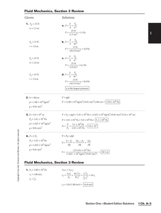
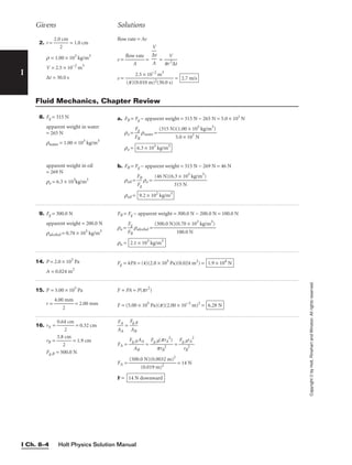
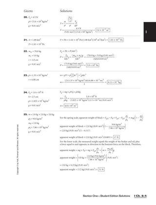
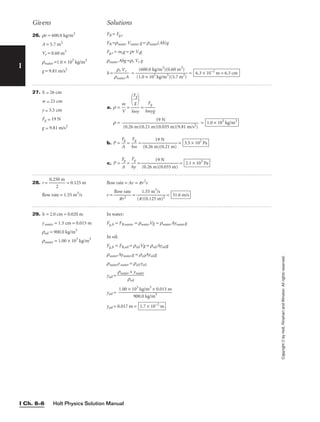
![Section One—Student Edition Solutions I Ch. 8–7
I
Copyright
©
by
Holt,
Rinehart
and
Winston.
All
rights
reserved.
Givens Solutions
31. k = 90.0 N/m
mb = 2.00 g
V = 5.00 m3
g = 9.81 m/s2
rair = 1.29 kg/m3
rhel = 0.179 kg/m3
Fnet = FB − Fg,b − Fg,hel − Fspring = 0
rairVg − mbg − rhelVg − k∆x = 0
∆x =
∆x =
∆x =
∆x = = 0.605 m
(9.81 m/s2
)(5.55 kg)
90.0 N/m
(9.81 m/s2
)(6.45 kg − 2.00 × 10⁻³
kg − 0.895 kg)
90.0 N/m
(9.81 m/s2
)[(1.29 kg/m3
)(5.00 m3
) − 2.00 × 10⁻³
kg − (0.179 kg/m3)(5.00 m3)]
90.0 N/m
g(rairV − mb − rhelV)
k
32. A = 2.0 cm2
r = 1.0 g/cm3
v = 42 cm/s
A2 = 3.0 × 10³
cm2
a. flow rate = Av = (2.0 cm2
)(42 cm/s) = 84 cm3
/s
In g/s:
flow rate = (84 cm3
/s)(1.0 g/cm3
) =
b. Use the continuity equation.
v2 =
A
A
1v
2
1
=
(2.0
3.
c
0
m
×
2
1
)(
0
4
3
2
cm
cm
2
/s)
= 0.028 cm/s = 2.8 × 10⁻⁴
m/s
84 g/s
33. m = 1.0 kg
r = 0.10 m
h = 2.0 m
rwater = 1.00 × 10³
kg/m3
g = 9.81 m/s2
rair = 1.29 kg/m3
Fnet = (m + mair)a = FB − Fg,b − Fg,a
(m + mair)a = rwaterVg − g(m + mair)
a =
m
rw
+
ate
m
rV
ai
g
r
− g = − g =
3m
rw
+
ate
r
r(
a
4
ir
p
(
r
4
3
p
)g
r3
)
− g
a = − 9.81 m/s2
a = − 9.81 m/s2
a = − 9.81 m/s2
a = 41 m/s2
− 9.81 m/s2
= 31 m/s2
Use the following equation to find the speed of the ball as it exits the water.
Note that vi = 0.
vf
2
= vi
2
+ 2ah = 2ah
Use the following equation to find the maximum height of the ball above the water.
Note that vi = vf for the ball leaving the water.
vf
2
= vi
2
− 2g∆y = 0
∆y =
v
2
i
g
2
=
2
2
a
g
h
=
a
g
h
∆y =
(31
9
m
.8
/s
1
2
m
)(2
/s
.0
2
m)
= 6.3 m
(1.00 × 10³
kg/m3
)(4π)(0.10 m3
)(9.81 m/s2
)
3.0 kg
(1.00 × 10³
kg/m3
)(4p)(0.10 m)3
(9.81 m/s2
)
3.0 kg + 0.016 kg
(1.00 × 10³
kg/m3
)(4p)(0.10 m)3
(9.81 m/s2
)
(3)(1.0 kg) + (1.29 kg/m3)(4p)(0.10 m)3
rwater
4
3
pr3
g
m + rair
4
3
pr3](https://image.slidesharecdn.com/physicssolutions-230306125240-7bc050a7/85/physics-solutions-pdf-117-320.jpg)
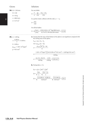
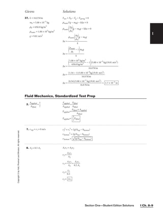
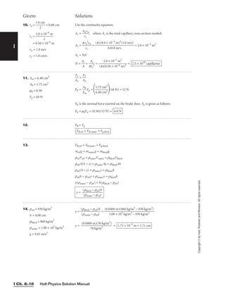


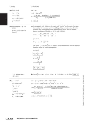

∆
Q
t
= (225 J/°C + 3.56 × 10³
J/°C)(1.5°C/min) = (3.78 × 10³
J/°C)(1.5°C/min)
∆
Q
t
=
or (5700 J/min)(1 min/60 s) = 95 J/s
5.7 × 10³
J/min
macp,a∆T + mwcp,w∆T
∆t
38.
TF =
9
5
TC + 32.0 TC = T − 273.15
TF − 32.0 =
9
5
TC
5
9
TF −
5
9
(32.0) = TC
5
9
TF −
5
9
(32.0) + 273.15 = T
T = TF
5
9
TF −
5
9
(32.0) + 273.15 = TF
5
9
TF − 17.8 + 273.15 = TF
5
9
TF + 255.4 = TF
255.4 =
4
9
TF
TF =
9
4
(255.4)°F = 574.6°F
TF = T
574.6°F = 574.6 K](https://image.slidesharecdn.com/physicssolutions-230306125240-7bc050a7/85/physics-solutions-pdf-127-320.jpg)
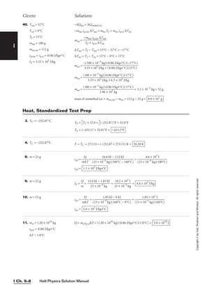

Q = (167 J/°C + 1260 J/°C)(2.0°C) = (1430 J/°C)(2.0°C) = 2900 J
16. TC = −40.0°C
TF =
9
5
TC + 32.0 =
9
5
(−40.0)°F + 32.0°F = (−72.0 + 32.0)°F
TF = −40.0°F](https://image.slidesharecdn.com/physicssolutions-230306125240-7bc050a7/85/physics-solutions-pdf-129-320.jpg)

![Section One—Student Edition Solutions I Ch. 10–1
Thermodynamics
Student Edition Solutions
I
1. P = 1.6 × 10⁵
Pa
Vi = 4.0 m3
2. P = 599.5 kPa
Vi = 5.317 × 10⁻⁴
m3
Vf = 2.523 × 10⁻⁴
m3
3. P = 4.3 × 10⁵
Pa
Vi = 1.8 × 10⁻⁴
m3
Vf = 9.5 × 10⁻⁴
m3
4. r =
1.6
2
cm
= 0.80 cm
d = 2.1 cm
W = 0.84 J
a. Vf = 2Vi = (2)(4.0 m3
) = 8.0 m3
W = P∆V = P(Vf − Vi) = (1.6 × 10⁵
Pa)(8.0 m3
− 4.0 m3
)
W = (1.6 × 10⁵
Pa)(4.0 m3
) =
b. Vf =
1
4
Vi =
1
4
(4.0 m3
) = 1.0 m3
W = P∆V = P(Vf − Vi) = (1.6 × 10⁵
Pa)(1.0 m3
− 4.0 m3
)
W = (1.6 × 10⁵
Pa)(−3.0 m3
) = −4.8 × 10⁵
J
6.4 × 10⁵
J
W = P∆V = P(Vf − Vi) = (599.5 × 10³
Pa)[(2.523 × 10⁻⁴
m3
) − (5.317 × 10⁻⁴
m3
)]
W = (599.5 × 10³
Pa)(−2.794 × 10⁻⁴
m3
) = −167.5 J
W = P∆V = P(Vf − Vi) = (4.3 × 10⁵
Pa)[(9.5 × 10⁻⁴
m3
) − (1.8 × 10⁻⁴
m3
)]
W = (4.3 × 10⁵
Pa)(7.7 × 10⁻⁴
m3
) = 3.3 × 10²
J
W = P∆V = PAd = Ppr2
d
P =
p
W
r2
d
= = 2.0 × 10⁵
Pa
0.84 J
p(0.80 × 10⁻²
m)2
(2.1 × 10⁻²
m)
Thermodynamics, Practice A
Givens Solutions
Copyright
©
by
Holt,
Rinehart
and
Winston.
All
rights
reserved.
2. A = 7.4 × 10⁻³
m2
d = −7.2 × 10⁻²
m
P = 9.5 × 10⁵
Pa
3. P = 1.5 × 10³
Pa
∆V = 5.4 × 10⁻⁵
m3
W = P∆V = PAd = (9.5 × 10⁵
Pa)(7.4 × 10⁻³
m2
)(−7.2 × 10⁻²
m) = −5.1 × 10²
J
W = P∆V = (1.5 × 10³
Pa)(5.4 × 10⁻⁵
m3
) = 8.1 × 10⁻²
J
Thermodynamics, Section 1 Review
1. W = 26 J
∆U = 7 J
∆U = Q − W
Q = W + ∆U = 26 J + 7 J = 33 J
Thermodynamics, Practice B](https://image.slidesharecdn.com/physicssolutions-230306125240-7bc050a7/85/physics-solutions-pdf-131-320.jpg)
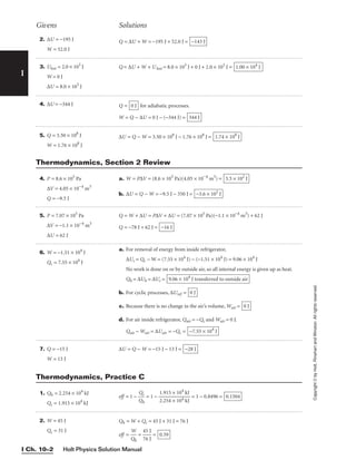
![Section One—Student Edition Solutions I Ch. 10–3
I
4. eff = 0.21
Qc = 780 J
5. W = 372 J
eff = 0.330
eff = 1 −
Q
Q
h
c
eff − 1 = −
Q
Q
h
c
1 − eff =
Q
Q
h
c
Qh =
1
Q
−
c
eff
=
1
7
−
8
0
0
.2
J
1
=
7
0
8
.7
0
9
J
= 990 J
W = Qh − Qc = 990 J − 780 J = 210 J
Qh = W + Qc
eff = 1 −
Q
Q
h
c
= 1 −
W
Q
+
c
Qc
=
W
W
+ Q
+
c
Q
−
c
Qc
=
W
W
+ Qc
W + Qc =
e
W
ff
Qc =
e
W
ff
− W =
e
1
ff
− 1
W =
0.3
1
30
− 1
(372 J)
Qc = (3.03 − 1)(372 J) = (2.03)(372 J) = 755 J
Givens Solutions
Copyright
©
by
Holt,
Rinehart
and
Winston.
All
rights
reserved.
2. Qh = 75 000 J
Qc = 35 000 J
a. W = Qh − Qc = 75 000 J − 35 000 J =
b. eff =
Q
W
h
=
4
7
.0
5
×
00
1
0
04
J
J
= 0.53
4.0 × 10⁴
J
Thermodynamics, Section 3 Review
9. Vi = 35.25 × 10⁻³
m3
Vf = 39.47 × 10⁻³
m3
P = 2.55 × 10⁵
Pa
10. P = 2.52 × 10⁵
Pa
Vi = 1.1 × 10⁻⁴
m3
Vf = 1.50 × 10⁻³
m3
W = P∆V = P(Vf − Vi) = (2.55 × 10⁵
Pa)[(39.47 × 10⁻³
m3
) − (35.25 × 10⁻³
m3
)]
W = (2.55 × 10⁵
Pa)(4.22 × 10⁻³
m3
) = 1.08 × 10³
J
W = P∆V = P(Vf − Vi)
W = (2.52 × 10⁵
Pa)(1.50 × 10⁻³
m3
− 1.1 × 10⁻⁴
m3
)
W = (2.52 × 10⁵
Pa)(1.4 × 10⁻³
m3
)
W = 3.5 × 10²
J
Thermodynamics, Chapter Review
3. Qh = 1.98 × 10⁵
J
Qc = 1.49 × 10⁵
J
a. eff = 1 −
Q
Q
h
c
= 1 −
1
1
.
.
4
9
9
8
×
×
1
1
0
0
5
5
J
J
= 1 − 0.753 =
b. W = Qh − Qc = (1.98 × 10⁵
J) − (1.49 × 10⁵
J) = 4.9 × 10⁴
J
0.247
6. Qc = 6.0 × 10²
J
eff = 0.31
Qh =
1
Q
−
c
eff
=
6
1
.0
−
×
0
1
.3
0
1
2
J
=
6.0
0
×
.6
1
9
02
J
= 8.7 × 10²
J](https://image.slidesharecdn.com/physicssolutions-230306125240-7bc050a7/85/physics-solutions-pdf-133-320.jpg)
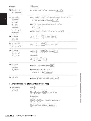


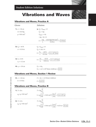

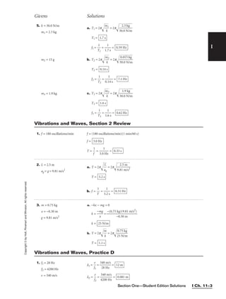
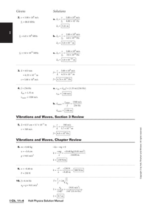


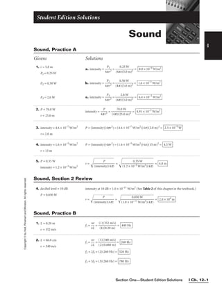


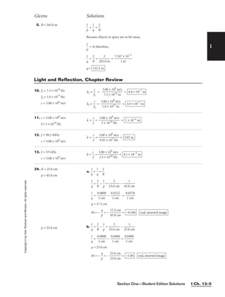


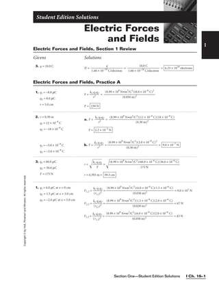

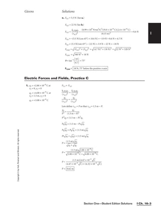
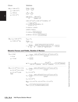

![Holt Physics Solution Manual
I Ch. 16–6
I
Copyright
©
by
Holt,
Rinehart
and
Winston.
All
rights
reserved.
2. r = 5.3 × 10⁻¹¹
m
q = 1.60 × 10⁻¹⁹
C
E =
k
r
C
2
q
= = 5.1 × 10¹¹
N/C
E = 5.1 × 10¹¹
N/C, away from the proton
(8.99 × 10⁹
N•m2
/C2
)(1.60 × 10⁻¹⁹
C)
(5.3 × 10⁻¹¹ m)2
3. E = 2.0 × 10⁴
N/C, along the
positive x-axis
qe = qp = 1.60 × 10⁻¹⁹
C
a. F = Eqe = (2.0 × 10⁴
N/C)(1.60 × 10−19
C)
F =
b. F = Eqp = (2.0 × 10⁴
N/C)(1.60 × 10−19
C)
F = 3.2 × 10⁻¹⁵
N, along the positive x-axis
3.2 × 10⁻¹⁵
N, along the negative x-axis
Givens Solutions
1. q1 = 40.0 × 10⁻⁹
C
q2 = 60.0 × 10⁻⁹
C
r =
30.0
2
cm
= 15.0 cm
E1 =
kC
r2
q1
= = 1.60 × 10⁴
N/C
E2 =
kC
r2
q2
= = 2.40 × 10⁴
N/C
Etot = E1 + E2 = (1.60 × 10⁴
N/C) − (2.40 × 10⁴
N/C) = −0.80 × 10⁴
N/C
Etot = 8.0 × 10³
N/C toward the 40.0 × 10⁻⁹
C charge
(8.99 × 10⁹
N•m2
/C2
)(60.0 × 10⁻⁹
C)
(0.150 m)2
(8.99 × 10⁹
N•m2
/C2
)(40.0 × 10⁻⁹
C)
(0.150 m)2
Electric Forces and Fields, Section 3 Review
3. q = 3.5 mC
N = = = 2.2 × 10¹³
electrons
3.5 × 10⁻⁶
C
1.60 × 10⁻¹⁹ C/electron
q
1.60 × 10⁻¹⁹
C/electron
Electric Forces and Fields, Chapter Review
15. q1 = q2 = (46)(1.60 × 10⁻¹⁹
C)
r = (2)(5.90 × 10⁻¹⁵
m)
F =
kC
r
q
2
1q2
=
F = 3.50 × 10³
N
(8.99 × 10⁹
N•m2
/C2
)[(46)(1.60 × 10⁻¹⁹
C)]2
[(2)(5.90 × 10⁻¹⁵
m)]2
16. q1 = 2.5 mC
q2 = −5.0 mC
r = 5.0 cm
F =
kC
r
q
2
1q2
=
F = 45 N
(8.99 × 10⁹
N•m2
/C2
)(2.5 × 10⁻⁶
C)(5.0 × 10⁻⁶
C)
(0.050 m)2
17. q1 = 2.0e
q2 = 79e
r = 2.0 × 10⁻¹⁴
m
e = 1.60 × 10⁻¹⁹
C
F =
kC
r
q
2
1q2
=
F = 91 N
(8.99 × 10⁹
N•m2
/C2
)(2.0)(79)(1.60 × 10⁻¹⁹
C)2
(2.0 × 10⁻¹⁴ m)2](https://image.slidesharecdn.com/physicssolutions-230306125240-7bc050a7/85/physics-solutions-pdf-186-320.jpg)


 = (3.0 × 10¹³
)(e)
Qnet = (3.0 × 10¹³
)(1.60 × 10⁻¹⁹
C)
Qnet = 4.8 × 10⁻⁶
C
35. a = 6.3 × 10³
m/s2
me = 9.109 × 10⁻³¹
kg
q = 1.60 × 10⁻¹⁹
C
a. F = mea = (9.109 × 10⁻³¹
kg)(6.3 × 10³
m/s2
) = 5.7 × 10⁻²⁷
N
F =
b. E =
F
q
=
1
5
.
.
6
7
0
×
×
1
1
0
0
−
−
2
1
7
9
N
C
= 3.6 × 10⁻⁸
N/C
5.7 × 10⁻²⁷
N, in a direction opposite E
36. 1.00 g of Cu has 9.48 × 10²¹
atoms.
1 Cu atom has 29 electrons.
a. 1.00 g of Cu has (9.48 × 10²¹
atoms)(29 electrons/atom) =
b. qtot = (2.75 × 10²³
electrons)(1.60 × 10⁻¹⁹
C/electron) = 4.40 × 10⁴
C
2.75 × 10²³
electrons](https://image.slidesharecdn.com/physicssolutions-230306125240-7bc050a7/85/physics-solutions-pdf-189-320.jpg)

![Section One—Student Edition Solutions I Ch. 16–11
I
Copyright
©
by
Holt,
Rinehart
and
Winston.
All
rights
reserved. 41. m1 = m2 = 0.20 g
q = 5.0°
L = 30.0 cm
ΣFy = 0 N, so Fg = FT,y = FT(cos 5.0°)
ΣFx = 0 N, so Felectric = FT,x = FT(sin 5.0°)
Fel
F
ec
g
tric
=
F
F
T
T
(
(
c
si
o
n
s
5
5
.
.
0
0
°
°
)
)
= tan 5.0°
r
k
2
C
m
q
g
2
= tan 5.0°
r = (2)(0.300 m)(sin 5.0°)
q =
r2
m
g(
t
k
a
C
n
5
.0
°)
q =
q = 7.2 × 10⁻⁹
C
[(2)(0.300 m)(sin 5.0°)]2
(0.20 × 10⁻³
kg)(9.81 m/s2
)(tan 5.0°)
8.99 × 10⁹ N•m2/C2
Givens Solutions
42. me = 9.109 × 10⁻³¹
kg
mp = 1.673 × 10⁻²⁷
kg
q = 1.60 × 10⁻¹⁹
C
a. F = Eq = mg
Ee =
m
q
eg
= = 5.58 × 10⁻¹¹
N/C
Ee =
b. Ep =
m
q
pg
= = 1.03 × 10⁻⁷
N/C
Ep = 1.03 × 10⁻⁷
N/C upward
(1.673 × 10⁻²⁷
kg)(9.81 m/s2
)
1.60 × 10⁻¹⁹ C
5.58 × 10⁻¹¹
N/C, downward
(9.109 × 10⁻³¹
kg)(9.81 m/s2
)
1.60 × 10⁻¹⁹ C
43. E = 520 N/C
∆t = 48 ns
vi = 0 m/s
me = 9.109 × 10⁻³¹
kg
mp = 1.673 × 10⁻²⁷
kg
q = 1.60 × 10⁻¹⁹
C
a =
m
F
=
q
m
E
vf = a∆t =
q
m
E
∆t
For the electron,
vf,e =
q
m
E∆
e
t
= =
For the proton,
vf,p =
q
m
E∆
p
t
= = 2.4 × 10³
m/s
(1.60 ×10⁻¹⁹
C)(520 N/C)(48 × 10−9
s)
1.673 × 10⁻²⁷ kg
4.4 × 10⁶
m/s
(1.60 ×10⁻¹⁹
C)(520 N/C)(48 × 10−9
s)
9.109 × 10⁻³¹ kg
44. E = 3.0 × 10⁴
N/C
q = 1.60 × 10⁻¹⁹
C
mp = 1.673 × 10⁻²⁷
kg
a. F = qE = (1.60 × 10⁻¹⁹
C)(3.0 × 10⁴
N/C) =
b. a =
m
F
p
= = 2.9 × 10¹²
m/s2
4.8 × 10⁻¹⁵
N
1.673 × 10⁻²⁷ kg
4.8 × 10⁻¹⁵
N](https://image.slidesharecdn.com/physicssolutions-230306125240-7bc050a7/85/physics-solutions-pdf-191-320.jpg)
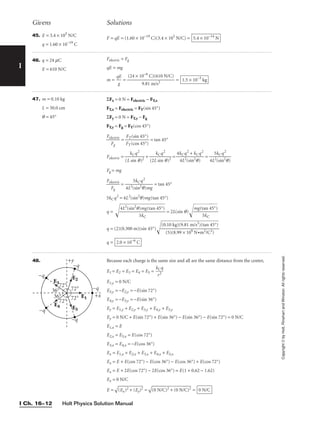
![Section One—Student Edition Solutions I Ch. 16–13
I
Copyright
©
by
Holt,
Rinehart
and
Winston.
All
rights
reserved.
Givens Solutions
49. E = 370.0 N/C
∆t = 1.00 ms
me = 9.109 × 10⁻³¹
kg
mp = 1.673 × 10⁻²⁷
kg
q = 1.60 × 10⁻¹⁹
C
ae =
m
F
e
=
m
qE
e
= = 6.50 × 10¹³
m/s2
∆xe =
1
2
ae∆t2
= (0.5)(6.50 × 10¹³
m/s2
)(1.00 × 10⁻⁶
s)2
= 32.5 m
ap =
m
F
p
=
m
qE
p
= = 3.54 × 10¹⁰
m/s2
∆xp =
2
1
ap∆t2
= (0.5)(3.54 × 10¹⁰
m/s2
)(1.00 × 10⁻⁶
s)2
∆xp = 1.77 × 10⁻²
m
∆xtot = ∆xe + ∆xp = 32.5 m + (1.77 × 10⁻²
m) = 32.5 m
(1.60 × 10⁻¹⁹
C)(370.0 N/C)
1.673 × 10⁻²⁷ kg
(1.60 × 10⁻¹⁹
C)(370.0 N/C)
9.109 × 10⁻³¹ kg
50. E = 300.0 N/C
me = 9.109 × 10⁻³¹
kg
q = 1.60 × 10⁻¹⁹
C
∆t = 1.00 × 10⁻⁸
s
a. a =
m
F
e
=
m
qE
e
= =
b. vf = a∆t = (5.27 × 10¹³
m/s2
)(1.00 × 10⁻⁸
s) = 5.27 × 10⁵
m/s
5.27 × 10¹³
m/s2
(1.60 × 10⁻¹⁹
C)(300.0 N/C)
9.109 × 10⁻³¹ kg
51. E = 3.0 × 10⁶
N/C
q = 1.60 × 10⁻¹⁹
C
me = 9.109 × 10⁻³¹
kg
vi = 0 m/s
vf = (0.100)(3.00 × 10⁸
m/s)
mp = 1.673 × 10⁻²⁷
kg
a. a =
m
F
e
=
m
qE
e
= =
b. vf
2
= 2a∆x
∆x =
v
2
f
a
2
= =
c. a =
m
F
p
=
m
qE
p
= = 2.9 × 10¹⁴
m/s2
(1.60 × 10⁻¹⁹
C)(3.0 × 10⁶
N/C)
1.673 × 10⁻²⁷ kg
8.5 × 10⁻⁴
m
[(0.100)(3.00 × 10⁸
m/s)]2
(2)(5.3 × 10¹⁷ m/s2)
5.3 × 10¹⁷
m/s2
(1.60 × 10⁻¹⁹
C)(3.0 × 10⁶
N/C)
9.109 × 10⁻³¹ kg
52. KE = 3.25 × 10⁻¹⁵
J
∆x = 1.25 m
vf = 0 m/s
q = 1.60 × 10⁻¹⁹
C
mp = 1.673 × 10⁻²⁷
kg
KE =
2
1
mpvi
2
vi =
2
m
K
p
E
a =
vf
2
2∆
−
x
vi
2
F = qE = mpa
E =
m
q
pa
=
(mp
(
)
q
(
)
v
(
f
2
2
∆
−
x)
vi
2
)
= =
mp
(q
v
)
f
(
2
2
−
∆
2
x
K
)
E
E = = −1.62 × 10⁴
N/C
E = 1.62 × 10⁴
N/C opposite the proton’s velocity
(1.673 × 10⁻²⁷
kg)(0 m/s)2
− (2)(3.25 × 10⁻¹⁵
J)
(1.60 × 10⁻¹⁹ C)(2)(1.25 m)
mpvf
2
− mp
2
m
K
p
E
2
(q)(2∆x)](https://image.slidesharecdn.com/physicssolutions-230306125240-7bc050a7/85/physics-solutions-pdf-193-320.jpg)
![Holt Physics Solution Manual
I Ch. 16–14
I
Copyright
©
by
Holt,
Rinehart
and
Winston.
All
rights
reserved.
Givens Solutions
53. m = 2.0 g
L = 20.0 cm
E = 1.0 × 10⁴
N/C
q = 15°
b. FT, y = Fg = mg
FT =
co
F
s
T
1
,y
5°
=
co
m
s 1
g
5°
qE = FT,x = FT(sin 15°) =
mg
c
(
o
s
s
in
15
1
°
5°)
= mg(tan 15°)
q =
mg(ta
E
n 15°)
= = 5.3 × 10⁻⁷
C
(2.0 × 10⁻³
kg)(9.81 m/s2
)(tan 15°)
1.0 × 10⁴ N/C
54. E = 2.0 × 10³
N/C along the
positive x-axis
q = 1.60 × 10⁻¹⁹
C
mp = 1.673 × 10⁻²⁷
kg
vf = 1.00 × 10⁶
m/s
a. F = qE = (1.60 × 10⁻¹⁹
C)(2.0 × 10³
N/C) = 3.2 × 10⁻¹⁶
N
F =
b. a =
m
F
p
=
1.
3
6
.
7
2
3
×
×
1
1
0
0
−
−
1
2
6
7
N
kg
=
c. ∆t =
v
a
f
= = 5.3 × 10⁻⁶
s
1.00 × 10⁶
m/s
1.9 × 10¹¹
m/s2
1.9 × 10¹¹
m/s2
3.2 × 10⁻¹⁶
N, along the positive x-axis
55. vf,1 = (0.010)(3.00 × 10⁸
m/s)
∆x1 = 2.0 mm
q = 1.60 × 10⁻¹⁹
C
me = 9.109 × 10⁻³¹
kg
∆x2 = 4.0 mm
a. a =
2
v
∆
f,1
x
2
1
E =
m
q
ea
=
m
2∆
ev
x
f
1
,1
q
2
E =
E =
b. a =
2
v
∆
f,1
x
2
1
= = 2.2 × 10¹⁵
m/s2
vf,2
2
= 2a∆x2
vf,2 =
2a
∆
x2
=
(2
)(
2.
2
×
1
01
5
m
/s
2)
(4
.0
×
1
0−
3
m
)
= 4.2 × 10⁶
m/s
[(0.010)(3.00 × 10⁸
m/s)]2
(2)(2.0 × 10⁻³ m)
1.3 × 10⁴
N/C
(9.109 × 10⁻³¹
kg)[(0.010)(3.00 × 10⁸
m/s)]2
(2)(2.0 × 10⁻³ m)(1.60 × 10⁻¹⁹ C)
56. r1 = 2.17 mm
q1 = 1.60 × 10⁻¹⁹
C
q2 = −1.60 × 10⁻¹⁹
C
r2 = (0.0100)(2.17 mm)
Felectric = Felastic
kC
r
q
1
1
2
q2
= kr2
k =
kC
r1
q
2
1
r
q
2
2
=
k = 2.25 × 10⁻⁹
N/m
(8.99 × 10⁹
N•m2/C2
)(1.60 × 10⁻¹⁹
C)2
(2.17 × 10⁻⁶ m)3(0.0100)](https://image.slidesharecdn.com/physicssolutions-230306125240-7bc050a7/85/physics-solutions-pdf-194-320.jpg)
![I
Copyright
©
by
Holt,
Rinehart
and
Winston.
All
rights
reserved.
Section One—Student Edition Solutions I Ch. 16–15
Electric Forces and Fields, Standardized Test Prep
Givens Solutions
11. q = 5.0 mC
r = 2.0 m
E1 = E2 = E3 =
k
r
C
2
q
= = 1.1 × 10⁴
N/C
Ex = (1.1 × 10⁴
N/C)(sin 60°) − (1.1 × 10⁴
N)(sin 60°) = 0.0 N/C
Ey = (1.1 × 10⁴
N/C) − (1.1 × 10⁴
N/C)(cos 60°) − (1.1 × 10⁴
N/C)(cos 60°)
Ey = (1.1 × 10⁴
N/C) − (5.5 × 10³
N/C) − (5.5 × 10³
N/C) = 0.0 N/C
Etot =
(0
.0
N
/C
)2
+
(
0.
0
N
/C
)2
= 0.0 N/C
(8.99 × 10⁹
N•m2/C2
)(5.0 × 10⁻⁶
C)
(2.0 m)2
13. q1 = (6.02 × 10²³
)(e)
q2 = (6.02 × 10²³
)(e)
r = (2)(6.38 × 10⁶
m)
e = 1.60 × 10⁻¹⁹
C
F =
kC
r
q
2
1q2
=
F = 5.12 × 10⁵
N
(8.99 × 10⁹
N•m2
/C2
)[(6.02 × 10²³
)(1.60 × 10⁻¹⁹
C)]2
[(2)(6.38 × 10⁶
m)]2
14. E = 3.0 × 10⁶
N/C
r = 2.0 m
q =
E
k
r
C
2
= = 1.3 × 10⁻³
C
(3.0 × 10⁶
N/C)(2.0 m)2
(8.99 × 10⁹ N•m2/C2)
15. E = 640 N/C
mp = 1.673 × 10⁻²⁷
kg
q = 1.60 × 10⁻¹⁹
C
a =
m
F
p
=
m
qE
p
= = 6.1 × 10¹⁰
m/s2
(1.60 × 10⁻¹⁹
C)(640 N/C)
1.673 × 10⁻²⁷ kg
16. vf = 1.20 × 10⁶
m/s
a = 6.1 × 10¹⁰
m/s2
∆t =
v
a
f
= = 2.0 × 10⁻⁵
s
1.20 × 10⁶
m/s
6.1 × 10¹⁰ m/s2
17. a = 6.1 × 10¹⁰
m/s2
∆t = 2.0 × 10⁻⁵
s
∆x =
1
2
a∆t2
= (0.5)(6.1 × 10¹⁰
m/s2
)(2.0 × 10⁻⁵
s)2
∆x = 12 m
18. mp = 1.673 × 10⁻²⁷
kg
vf = 1.20 × 10⁶
m/s
KEf =
1
2
mpvf
2
= (0.5)(1.673 × 10⁻²⁷
kg)(1.20 × 10⁶
m/s)2
KEf = 1.20 × 10⁻¹⁵
J](https://image.slidesharecdn.com/physicssolutions-230306125240-7bc050a7/85/physics-solutions-pdf-195-320.jpg)


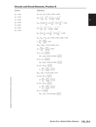


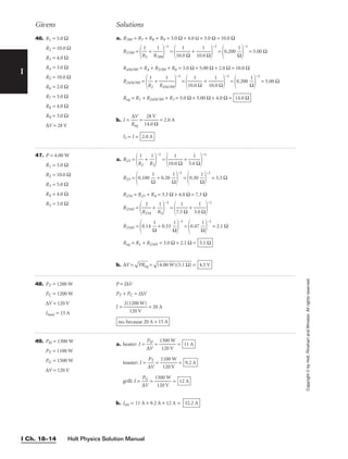
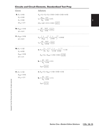


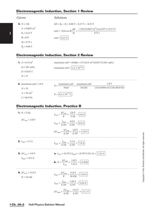
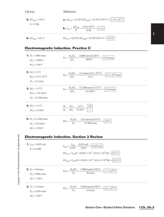
![I
Copyright
©
Holt,
Rinehart
and
Winston.
All
rights
reserved.
Holt Physics Solution Manual
I Ch. 20–4
12. N = 52
A = 5.5 × 10⁻³
m2
Bi = 0.00 T
Bf = 0.55 T
∆t = 0.25 s
q = 0.0°
emf =
−NA(c
∆
o
t
s q)∆B
∆B = Bf − Bi = 0.55 T − 0.00 T = 0.55 T
emf = = −0.63 V
−(52)(5.5 × 10⁻³
m2
)(cos 0.0°)(0.55 T)
0.25 s
26. ∆Vrms = 220 000 V ∆Vmax =
∆
0.
V
7
r
0
m
7
s
=
22
0
0
.7
0
0
0
7
0 V
= 310 000 V = 3.1 × 10⁵
V
10. N = 1
ri = 0.12 m
B = 0.15 T
Af = 3 × 10⁻³
m2
∆t = 0.20 s
q = 0.0°
emf =
−N(co
∆
s
t
q)B∆A
∆A = Af − Ai = Af − pri
2
= (3 × 10⁻³
m2
) − (p)(0.12 m)2
∆A = (3 × 10⁻³
m2
) − 0.045 m2
= −0.042 m2
emf = = 3.2 × 10⁻²
V
−(1)(cos 0.0°)(0.15 T)(−0.042 m2
)
0.20 s
27. ∆Vmax = 340 V
R = 120 Ω
a. ∆Vrms = (0.707)(∆Vmax) = (0.707)(340 V) =
b. Irms =
∆V
R
rms
=
2.40
12
×
0
1
Ω
02
V
= 2.0 A
2.4 × 10²
V
Electromagnetic Induction, Chapter Review
Givens Solutions
11. A = (0.055 m)(0.085 m)
q = 0.0°
N = 75
R = 8.7 Ω
−
∆
∆
t
B
= 3.0 T/s
emf = −N
∆[AB(
∆
c
t
os q)]
= −NA(cos q)
∆
∆
B
t
emf = −(75)(0.055 m)(0.085 m)(cos 0.0°)(−3.0 T/s) = 1.05 V
I =
em
R
f
=
1
8
.
.
0
7
5
Ω
V
= 0.12 A
28. Imax = 0.909 A
R = 182 Ω
a. Irms = (0.707)(Imax) = (0.707)(0.909 A) =
b. ∆Vrms = IrmsR = (0.643 A)(182 Ω) =
c. P = Irms
2
R = (0.643 A)2
(182 Ω) = 75.2 W
117 V
0.643 A
29. P = 996 W
Imax = 11.8 A
a. Irms = (0.707)(Imax) = (0.707)(11.8 A) =
b. ∆Vrms =
Ir
P
ms
=
9
8
9
.3
6
4
W
A
= 119 V
8.34 A](https://image.slidesharecdn.com/physicssolutions-230306125240-7bc050a7/85/physics-solutions-pdf-232-320.jpg)
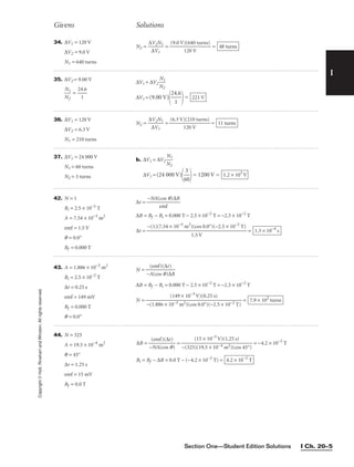

![Section One—Student Edition Solutions I Ch. 20–7
I
Copyright
©
Holt,
Rinehart
and
Winston.
All
rights
reserved.
4. ∆Vrms =
∆V
m
2
ax
∆
∆
V
V
m
rm
ax
s
=
1
2
6. A2 = 1.5A1
B2 = B1
N2 = 2N1
cos q2 = cos q1
∆t2 = 0.5∆t1
∆V1 = −
N1∆[A
∆
1B
t1
1cosq1]
∆V2 = −
N2∆[A
∆
2B
t2
2cosq2]
∆
∆
V
V
2
1
=
N
N
2
1
∆
∆
[
[
A
A
2
1
B
B
2
1
c
c
o
o
s
s
q
q
2
1
]
]
∆
∆
t
t
1
2
∆
∆
V
V
2
1
=
N
N
2
1
A
A
2
1
∆
∆
t
t
1
2
=
N
N
2
1
A
A
2
1
∆
∆
t
t
1
2
∆
∆
V
V
2
1
=
2
N
N
1
1
1.
A
5A
1
1
0.
∆
5∆
t1
t1
=
2
1
1
1
.5
0
1
.5
= 6
∆V2 = 6 × ∆V1
Electromagnetic Induction, Standardized Test Prep
Givens Solutions
8. ∆V1 = 240 000 V
N1A = 1000 turns
N2A = 50 turns
N1B = 600 turns
N2B = 20 turns
∆V2 = ∆V1
N
N
2
1
A
A
N
N
2
1
B
B
∆V2 = (240 000V)
1
5
0
0
00
tu
tu
rn
rn
s
s
6
2
0
0
0
t
t
u
u
r
r
n
n
s
s
= 400 V
10. Imax = 3.5 A
∆Vmax = 340 V
Irms = 0.707Imax = (0.707)(3.5 A) = 2.5 A
∆Vrms = 0.707∆Vmax = (0.707)(340 V) = 240 V
Pdissipated = ∆VrmsIrms = (240 V)(2.5 A) = 600 W
11. Imax = 12.0 A Irms = 0.707Imax = (0.707)(12.0 A) = 8.48 A
14. N1 = 150 turns
N2 = 75 000 turns
∆V1 = 120 V
∆V2 = ∆V1
N
N
2
1
= (120 V)
75
15
0
0
00
tu
t
r
u
n
r
s
ns
∆V2 = 6.0 × 10⁴
V
18.
∆
∆
B
t
= 0.10 T/s
r = 2.4 cm = 0.024 m
N = 1
q = 180° (for maximum
emf)
emf = − N
∆
∆
Φ
t
M
= −
N∆[AB
∆t
cos q]
emf = − NA cos q
∆
∆
B
t
= − Nπr2
cos q
∆
∆
B
t
emf = − (1)(π)(0.024 m)2
(cos 180°)(0.10 T/s)
emf = 1.8 × 10⁻⁴
V](https://image.slidesharecdn.com/physicssolutions-230306125240-7bc050a7/85/physics-solutions-pdf-235-320.jpg)

6.63 × 10⁻³⁴ J•s
Atomic Physics, Practice B
Atomic Physics
Student Edition Solutions
2. l = 350 nm
KEmax = 1.3 eV
work function = hf − KEmax
f =
l
c
work function = h
l
c
− KEmax
work function = − 1.3 eV
work function = 3.6 eV − 1.3 eV =
ft =
work f
h
unction
=
ft = 5.6 × 10¹⁴
Hz
(2.3 eV)(1.60 × 10⁻¹⁹
J/eV)
6.63 × 10⁻³⁴ J•s
2.3 eV
(6.63 × 10⁻³⁴
J•s)(3.00 × 10⁸
m/s)
(1.60 × 10⁻¹⁹ J/eV)(350 × 10−9 m)](https://image.slidesharecdn.com/physicssolutions-230306125240-7bc050a7/85/physics-solutions-pdf-236-320.jpg)
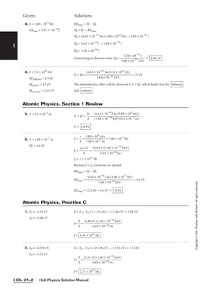


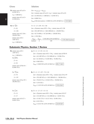


![I
Givens Solutions
Copyright
©
by
Holt,
Rinehart
and
Winston.
All
rights
reserved.
Holt Physics Solution Manual
V Apx I–2
9. vi = 4.0 m/s
∆t = 18 s
∆x = 135 m
vf =
2
∆
∆
t
x
− vi =
(2)(
1
1
8
35
s
m)
− 4.0 m/s = 15 m/s − 4.0 m/s =
vf = (11 m/s)
36
1
0
h
0 s
1
1
0
k
3
m
m
vf = 4.0 × 101
km/h
11 m/s
10. vi = 7.0 km/h
vf = 34.5 km/h
∆x = 95 m
a =
vf
2
2
−
∆x
vi
2
=
a =
a = = 0.46 m/s2
(1140 km2
/h2
)
36
1
0
h
0 s
2
1
1
0
k
3
m
m
2
190 m
(1190 km2
/h2
− 49 km2
/h2
)
36
1
0
h
0 s
2
1
1
0
k
3
m
m
2
190 m
[(34.5 km/h)2
− (7.0 km/h)2
]
36
1
0
h
0 s
2
1
1
0
k
3
m
m
2
(2)(95 m)
11. ∆x = 4.0 m
∆t = 5.0 min
vavg =
∆
∆
x
t
= = 48 m/h
4.0 m
(5.0 min)
60
1
m
h
in
12. ∆t = 28 s
a = 0.035 m/s2
vi = 0.76 m/s
vf = a∆t + vi = (0.035 m/s2
)(28.0 s) + 0.76 m/s = 0.98 m/s + 0.76 m/s = 1.74 m/s
13. ∆ttot = 5.10 s
a = −9.81 m/s2
∆xtot = 0 m
∆ttot = vi ∆ ttot +
1
2
a∆ttot
2
Because ∆xtot = 0,
vi = −
1
2
a∆ttot = −
1
2
(−9.81 m/s2
)(5.10 s) = +25.0 m/s = 25.0 m/s upward
14. aavg = −0.870 m/s2
∆t = 3.80 s
aavg =
∆
∆
va
t
vg
∆vavg = aavg∆t = (−0.870 m/s2
)(3.80 s) = −3.31 m/s
15. ∆x = 55.0 m
∆t = 1.25 s
vf = 43.2 m/s
vi =
2
∆
∆
t
x
− vf =
(2)
1
(5
.2
5
5
.0
s
m)
− 43.2 m/s = 88.0 m/s − 43.2 m/s = 44.8 m/s
16. ∆x = 12.4 m upward
∆t = 2.0 s
vi = 0 m/s
Because vi = 0 m/s, a =
2
∆
∆
t2
x
=
(2)
(
(
2
1
.0
2.
s
4
)2
m)
= 6.2 m/s2
upward](https://image.slidesharecdn.com/physicssolutions-230306125240-7bc050a7/85/physics-solutions-pdf-255-320.jpg)
![I
Givens Solutions
Copyright
©
by
Holt,
Rinehart
and
Winston.
All
rights
reserved.
Section One—Student Edition Solutions V Apx I–3
17. ∆x = +42.0 m
vi = +153.0 km/h
vf = 0 km/h
a =
vf
2
2∆
−
x
vi
2
=
a = = −21.5 m/s2
−(2.34 × 10⁴
km2
/h2
)
36
1
0
h
0 s
2
1
1
0
k
3
m
m
2
(84.0 m)
[(0 km/h)2
− (153.0 km/h)2
]
36
1
0
h
0 s
2
1
1
0
k
3
m
m
2
(2) (42.0 m)
18. vi = 17.5 m/s
vf = 0.0 m/s
∆ttot = 3.60 s
∆x =
1
2
(vi + vf)∆t
∆ttop =
∆t
2
tot
=
3.6
2
0 s
= 1.80 s
∆x =
1
2
(17.5 m/s + 0.0 m/s)(1.80 s) = 15.8 m
19. ∆t = 5.50 s
vi = 0.0 m/s
vf = 14.0 m/s
∆x =
1
2
(vi + vf)∆t =
1
2
(0.0 m/s + 14.0 m/s)(5.50 s) = 38.5 m
20. v = 6.50 m/s downward
= −6.50 m/s
∆t = 34.0 s
∆x = v∆t = (−6.50 m/s)(34.0 s) = −221 m = 221 m downward
21. vt = 10.0 cm/s
vh = 20 vt = 2.00 × 10²
cm/s
∆trace = ∆tt
∆th = ∆tt − 2.00 min
∆xt = ∆xh + 20.0 cm = ∆xrace
∆xt = vt∆tt
∆xh = vh∆th = vh (∆tt − 2.00 min)
∆xt = ∆xrace = ∆xh + 20.0 cm
vt ∆tt = vh (∆tt − 2.00 min) + 20.0 cm
∆tt (vt − vh) = −vh (2.00 min) + 20.0 cm
∆tt =
∆trace = ∆tt =
∆trace = =
∆trace = 126 s
−2.40 × 10⁴
cm
−1.90 × 10²
cm/s
20.0 cm − 2.40 × 10⁴
cm
−1.90 × 10²
cm/s
20.0 cm − (2.00 × 10²
cm/s)(2.00 min)(60 s/min)
10.0 cm/s − 2.00 × 10²
cm/s
20.0 cm − vh (2.00 min)
vt − vh
22. ∆xrace = ∆xt
vt = 10.0 cm/s
∆tt = 126 s
∆xrace = ∆xt = vt∆tt = (10.0 cm/s)(126 s) = 1.26 × 10³
cm = 12.6 m
23. vi = 12.5 m/s up,
vi = +12.5 m/s
vf = 0 m/s
a = 9.81 m/s2
down,
a = −9.81 m/s2
vf = vi + a∆t
∆t =
vf
a
− vi
=
0 m
−
/
9
s
.8
−
1
1
m
2.5
/s2
m/s
= 1.27 s](https://image.slidesharecdn.com/physicssolutions-230306125240-7bc050a7/85/physics-solutions-pdf-256-320.jpg)
![I
Givens Solutions
Copyright
©
by
Holt,
Rinehart
and
Winston.
All
rights
reserved.
Holt Physics Solution Manual
V Apx I–4
24. ∆t = 0.910 s
∆x = 7.19 km
vi = 0 km/s
vf =
2
∆
∆
t
x
− vi =
(2)
0
(7
.9
.1
1
9
0
k
s
m)
− 0 km/s = 15.8 km/s
25. a = 3.0 m/s2
∆t = 4.1 s
vf = 55.0 km/h
vf = vi + a∆t
vi = vf − a∆t =
55.0
h
km
−(3.0 m/s2
)(4.1 s)
1
1
00
k
0
m
m
36
1
0
h
0 s
vi = 55.0 km/h − 44 km/h = 11 km/h
26. ∆t = 1.5 s
vi = 2.8 km/h
vf = 32.0 km/h
a = =
a = = 5.4 m/s2
(29.2 km/h)
36
1
0
h
0 s
1
1
0
k
3
m
m
1.5 s
(32.0 km/h − 2.8 km/h)
36
1
0
h
0 s
10
k
3
m
m
1.5 s
vf − vi
∆t
27. a = 4.88 m/s2
∆x = 18.3 m
vi = 0 m/s
Because vi = 0 m/s,
∆t =
2∆
a
x
= = 2.74 s
(2)(18.3 m)
(4.88 m/s2
)
28. aavg = 16.5 m/s2
vi = 0 km/h
vf = 386.0 km/h
∆t = = =
∆t = = 6.50 s
107.2 m/s
16.5 m/s2
(386.0 km/h − 0 km/h)
36
1
0
h
0 s
1
1
0
k
3
m
m
16.5 m/s2
vf − vi
aavg
∆v
aavg
29. vi = 50.0 km/h forward
= +50.0 km/h
vf = 0 km/h
a = 9.20 m/s2
backward
= −9.20 m/s2
∆x =
vf
2
2
−
a
vi
2
=
∆x =
∆x = 10.5 m = 10.5 m forward
−(2.50 × 10³
km2
/h2
)
36
1
0
h
0 s
2
1
1
0
k
3
m
m
2
−18.4 m/s2
[(0 km/h)2
− (50.0 km/h)2
]
36
1
0
h
0 s
2
1
1
0
k
3
m
m
2
(2)(−9.20 m/s2
)
30. vi = −4.0 m/s
aavg = −0.27 m/s2
∆t = 17 s
vf = aavg ∆t + vi
vf = (−0.27 m/s2
)(17 s) + (−4.0 m/s) = −4.6 m/s − 4.0 m/s = −8.6 m/s
31. vi = +4.42 m/s
vf = 0 m/s
a = −0.75 m/s2
∆t =
vf −
a
vi
=
0 m
−
/
0
s
.7
−
5
4
m
.42
/s2
m/s
=
−
−
0
4
.
.
7
4
5
2
m
m
/
/
s
s
2
= 5.9 s](https://image.slidesharecdn.com/physicssolutions-230306125240-7bc050a7/85/physics-solutions-pdf-257-320.jpg)

![I
Givens Solutions
Copyright
©
by
Holt,
Rinehart
and
Winston.
All
rights
reserved.
Section One—Student Edition Solutions V Apx I–7
48. d = 478 km
∆y = 42 km, south = −42 km
d2
= ∆x2
+ ∆y2
∆x =
d
2
−
∆
y2
=
(4
78
k
m
)2
−
(
−
42
k
m
)2
2.
28
×
1
05
k
m
2
−
1
.8
×
1
03
k
m
2
∆x =
2.
26
×
1
05
k
m
2
= −475 km
∆x = 475 km, west
49. d = 478 km
∆y = 42 km, south = −42 km
q = sin−1
∆
d
y
= sin−1
−
47
4
8
2
k
k
m
m
q = 5.0° south of west
50. d = 7400 km
q = 26° south of west
∆y = 3200 km, south =
−3200 km
d2
= ∆x2
= ∆y2
∆x =
d
2
−
∆
y2
=
(7
40
0
km
)2
−
(
−
32
00
k
m
)2
=
5.
5
×
1
07
k
m
2
−
1
.0
×
1
07
k
m
2
∆x =
4.
5
×
1
07
k
m
2
= −6700 km
∆x = 6700 km, west
51. d = 5.3 km
q = 8.4° above horizontal
∆y = d(sin q) = (5.3 km)(sin 8.4°)
∆y = 0.77 km = 770 m
the mountain’s height = 770 m
52. d = 113 m
q = 82.4° above the
horizontal south
∆x = d(cos q) = (113 m)(cos 82.4°)
∆x = 14.9 m, south
53. v = 55 km/h
q = 37° below the horizontal
= −37°
vy = v(sin q) = (55 km/h)[sin(−37°)]
vy = −33 km/h = 33 km/h, downward](https://image.slidesharecdn.com/physicssolutions-230306125240-7bc050a7/85/physics-solutions-pdf-260-320.jpg)
![I
Givens Solutions
Copyright
©
by
Holt,
Rinehart
and
Winston.
All
rights
reserved.
Section One—Student Edition Solutions V Apx I–11
69. d1 = 46 km
q1 = 15° south of east
= −15°
d2 = 22 km
q2 = 13° east of south
= −77°
d3 = 14 km
q3 = 14° west of south
= −90.0° − 14° = −104°
∆x1 = d1(cos q1) = (46 km)[cos(−15°)] = 44 km
∆y1 = d1(sin q1) = (46 km)[sin(−15°)] = −12 km
∆x2 = d2(cos q2) = (22 km)[cos(−77°)] = 4.9 km
∆y2 = d2(sin q2) = (22 km)[sin(−77°)] = −21 km
∆x3 = d3(cos q3) = (14 km)[cos(−104°)] = −3.4 km
∆y3 = d3(sin q3) = (14 km)[sin(−104°)] = −14 km
∆xtot = ∆x1 + ∆x2 + ∆x3 = 44 km + 4.9 km + (−3.4 km) = 46 km
∆ytot = ∆y1 + ∆y2 + ∆y3 = −12 km + (−21 km) + (−14 km) = −47 km
d =
(∆
xt
ot
)2
+
(
∆
yt
ot
)2
=
(4
6
km
)2
+
(
−
47
k
m
)2
=
2.
1
×
1
03
k
m
2
+
2
.2
×
1
03
k
m
2
=
4.
3
×
1
03
k
m
2
d =
q = tan−1
∆
∆
x
yt
t
o
o
t
t
= tan−1
−
4
4
6
7
k
k
m
m
= −46°
q = 46° south of east
66 km
70. vx = 9.37 m/s ∆t =
∆
vx
x
∆x = 85.0 m
∆y = −
1
2
g∆t2
g = 9.81 m/s2
∆y = −
1
2
g
∆
vx
x
2
= −
1
2
(9.81 m/s2
)
9
8
.3
5
7
.0
m
m
/s
2
= − 404 m
71. ∆y = −2.50 × 10²
m ∆x = vx∆t
vx = 1.50 m/s ∆y = −
1
2
g∆t2
g = 9.81 m/s2
∆t =
2
−
∆
g
y
∆x = vx
2
−
∆
g
y
= (1.50 m/s)
(2
)(
−
−
2
9
.
.
5
8
0
1
×
m
1
/
0
s2
2
m
)
∆x =
72. vx = 1.50 m/s vy,f
2
= −2g∆y + vy,i
2
∆y = −2.50 × 10²
m vy,i = 0 m/s, so
g = 9.81 m/s2
vy,f = vy =
−
2g
∆
y
=
−
(2
)(
9.
81
m
/s
2
)
(−
2.
50
×
1
02
m
)
vy = 70.0 m/s
v =
vx
2
+
v
y
2
=
(1
.5
0
m
/s
)2
+
(
70
.0
m
/s
)2
=
2.
25
m
2
/
s2
+
4
.9
0
×
1
03
m
2
/
s2
=
4.
90
×
1
03
m
2
/
s2
v =
q = tan−1
v
v
x
y
= tan−1
1
7
.
0
5
.
0
0
m
m
/
/
s
s
q = 1.23° from the vertical
70.0 m/s
10.7 m
mountain’s height = 404 m](https://image.slidesharecdn.com/physicssolutions-230306125240-7bc050a7/85/physics-solutions-pdf-264-320.jpg)
![I
Givens Solutions
Copyright
©
by
Holt,
Rinehart
and
Winston.
All
rights
reserved.
Holt Physics Solution Manual
V Apx I–12
73. q = −30.0° ∆y = vi(sin q)∆t −
1
2
g∆t2
vi = 2.0 m/s
2
g
∆t2
− [vi(sin q)]∆t + ∆y = 0
∆y = −45 m
Solving for ∆t using the quadratic equation,
g = 9.81 m/s2
∆t =
∆t =
∆t = =
∆t =
∆t must be positive, so the positive root must be chosen.
∆t =
9.
2
8
9
1
m
m
/
/
s
s2
=
74. vi = 10.0 m/s ∆x = vi(cos q)∆t = (10.0 m/s)(cos 37.0°)(2.5 s)
q = 37.0° ∆x =
∆t = 2.5 s ∆y = vi(sin q)∆t −
1
2
g∆t2
= (10.0 m/s)(sin 37.0°)(2.5 s) −
1
2
(9.81 m/s2
)(2.5 s)2
g = 9.81 m/s2
= 15 m − 31 m
∆y =
75. vaw = 55.0 km/h, north vae = vaw + vwe
vwe = 40.0 km/h at 17.0° vx, ae = vx, aw + vx, we = vwe (cos qwe)
north of west vy, ae = vy, aw + vy, we = vaw + vwe(sin qwe)
qwe = 180.0° − 17.0° = 163.0°
vx, ae = (40.0 km/h)(cos 163.0°) = −38.3 km/h
vy, ae = 55.0 km/h + (40.0 km/h)(sin 163.0°) = 55.0 km/h + 11.7 km/h = 66.7 km/h
vae =
vx
, a
e)
2
+
(
vy
, a
e0
2
=
(−
38
.3
k
m
/h
)2
+
(
66
.7
k
m
/h
)2
vae =
1.
47
×
1
03
k
m
2
/
h
2
+
4
.4
5
×
1
03
k
m
2
/
h
2
=
5.
92
×
1
03
k
m
2
/
h
2
vae =
q = tan−1
v
v
x
y,
,
a
a
e
e
= tan−1
= −60.1°
q = 60.1° west of north
66.7 km/h
−38.3 km/h
76.9 km/h
−16 m
2.0 101
m
3.0 s
−1.0 m/s ± 3.0 × 101
m/s
9.81 m/s2
−1.0 m/s ±
8.
8
×
1
02
m
2
/
s2
9.81 m/s2
−1.0 m/s ±
1.
0
m
2
/
s2
+
8
.8
×
1
02
m
2
/
s2
9.81 m/s2
(2.0 m/s)[sin(−30.0°)] ±
[(
−
2.
0
m
/s
)[
si
n
(−
30
.0
°)
]2
−
(
2)
(9
.8
1
m
/s
2
)
(−
45
m
)
9.81 m/s2
vi(sin q) ±
[−
vi
(s
in
q
)]
2
−
4
2
g
(
∆
y)
2
2
g
](https://image.slidesharecdn.com/physicssolutions-230306125240-7bc050a7/85/physics-solutions-pdf-265-320.jpg)

![I
Givens Solutions
Copyright
©
by
Holt,
Rinehart
and
Winston.
All
rights
reserved.
Holt Physics Solution Manual
V Apx I–14
79. vx = 85.3 m/s ∆t =
2
−
∆
g
y
=
∆
vx
x
∆y = −1.50 m
∆x = vx
2
−
∆
g
y
= (85.3 m/s)
(2
−
)
9
(
.
−
8
1
1
.
5
m
0
/
m
s2
)
= 47.2 m
g = 9.81 m/s2
range of arrow = 47.2 m
80. ∆t = 0.50 s
∆x = 1.5 m
q = 33°
∆x = vi(cos q)∆t
vi =
(cos
∆
q
x
)∆t
=
(cos 3
1
3
.
°
5
)
m
(0.50 s)
= 3.6 m/s
81. ∆x1 = 0.46 m ∆xtot = ∆x1 + ∆x2
∆x2 = 4.00 m ∆t =
vi(c
∆
o
x
s q)
q = 41.0° ∆y = vi(sin q)∆t −
1
2
g∆t2
= vi(sin q)
∆
vi
x
(
i
c
+
os
∆
q
x
)
2
−
1
2
g
∆
v
x
i(
1
co
+
s
∆
q
x
)
2
2
∆y = − 0.35 m ∆y = (∆x1 + ∆x2)(tan q) −
g
2
(∆
v
x
i
2
1
(c
+
o
∆
s
x
q
2
)2
)2
g = 9.81 m/s2
vi =
vi =
vi =
vi =
vi = 6.36 m/s
(9.81 m/s2
)(4.46 m)2
(2)(cos 41.0°)2
(4.23 m)
(9.81 m/s2
)(4.46 m)2
(2)(cos 41.0°)2
(3.88 m + 0.35 m)
(9.81 m/s2
)(0.46 m + 4.00 m)2
(2)(cos 41.0°)2
[(0.46 m + 4.00 m)(tan 41.0°) − (−0.35 m)]
g(∆x1 + ∆x2)2
2(cos q)2
[(∆x1 + ∆x2)(tan q) − ∆y]
82. vfc = 87 km/h, west vfe = vfc + vce
vce = 145 km/h, north vx, fe = vx, fc + vx, ce = vfc = −87 km/h
∆t = 0.45 s vy, fe = vy, fc + vy, ce = vce = +145 km/h
∆x = vx, fe ∆t = (−87 km/h)(103
m/km)(1 h/3600 s)(0.45 s) = −11 m
∆x =
∆y = vy, fe ∆t = (145 km/h)(103
m/km)(1 h/3600 s)(0.45 s)
∆y = 18 m, north
11m, west](https://image.slidesharecdn.com/physicssolutions-230306125240-7bc050a7/85/physics-solutions-pdf-267-320.jpg)
![I
Givens Solutions
Copyright
©
by
Holt,
Rinehart
and
Winston.
All
rights
reserved.
Section One—Student Edition Solutions V Apx I–15
83. vbw = 12.0 km/h, south vbe = vbw + vwe
vwe = 4.0 km/h at 15.0° vx, be = vx, bw + vx, we = vwe(cos qwe)
south of east vy, be = vy, bw + vy, we = vbw + vwe(sin qwe)
qwe = −15.0°
vx, be = (4.0 km/h)[cos(−15.0°)] = 3.9 km/h
vy, be = (−12.0 km/h) + (4.0 km/h)[sin(−15.0°)] = (−12.0 km/h) + (−1.0 km/h)
= −13.0 km/h
vbe =
(v
x,
b
e)
2
+
v
y,
be
)2
=
(3
.9
k
m
/h
)2
+
(
−
13
.0
k
m
/h
)2
vbe =
15
k
m
2
/
h
2
+
1
69
k
m
2
/
h
2
=
18
4
km
2
/
h
2
vbe =
q = tan−1
v
v
x
y,
,
b
b
e
e
= tan−1
−
3
1
.
3
9
.0
km
km
/h
/h
= −73°
q = 73° south of east
13.6 km/h
Forces and the Laws of Motion
84. F1 = 7.5 × 10⁴
N north
F2 = 9.5 × 10⁴
N at 15.0°
north of west
q1 = 90.0°
q2 = 180.0° − 15.0° = 165.0°
Fx,net = Fx = F1(cos q1) + F2(cos q2)
Fx,net = (7.5 × 10⁴
N)(cos 90.0°) + (9.5 × 10⁴
N)(cos 165.0°)
Fx,net = −9.2 × 10⁴
N
Fy,net = Fy = F1(sin q1) + F2(sin q2)
Fy,net = (7.5 × 10⁴
N)(sin 90.0°) + (9.5 × 10⁴
N)(sin 165.0°)
Fy,net = 7.5 × 10⁴
N + 2.5 × 10⁴
N = 10.0 × 10⁴
N
q = tan−1
= tan−1
= −47°
q = 47° north of west
10.0 × 10⁴
N
−9.2 × 10⁴
Fy,net
Fx,net
85. F = 76 N
q = 40.0°
Fx = F(cos q) = (76 N)(cos 40.0°)
Fx = 58 N
86. F = 76 N
q = 40.0°
Fy = F(sin q) = (76 N)(sin 40.0°)
Fy = 49 N
87. F1 = 6.0 N
F2 = 8.0 N
Fmax = F1 + F2 = 6.0 N + 8.0 N
Fmax =
Fmin = F2 − F1 = 8.0 N − 6.0 N
Fmin = 2.0 N
14.0 N
88. m = 214 kg
Fbuoyant = 790 N
g = 9.81 m/s2
Fnet = Fbuoyant − mg = 790 N − (214 kg)(9.81 m/s2
)
Fnet = 790 N − 2.10 × 10³
N = −1310 N
anet = = = −6.12 m/s2
−1310 N
214 kg
Fnet
m](https://image.slidesharecdn.com/physicssolutions-230306125240-7bc050a7/85/physics-solutions-pdf-268-320.jpg)

![I
Givens Solutions
Copyright
©
by
Holt,
Rinehart
and
Winston.
All
rights
reserved.
Section One—Student Edition Solutions V Apx I–17
96. Fapplied = 5.0 N to the left
m = 1.35 kg
anet = 0.76 m/s2
to the left
Fnet = m anet = Fapplied − Fk
Fk = Fapplied − m anet
Fk = 5.0 N − (1.35 kg)(0.76 m/s2
) = 5.0 N − 1.0 N = 4.0 N
Fk = 4.0 N to the right
97. F1 = 15.0 N
q = 55.0°
Fy = F(sin q) = (15.0 N)(sin 55.0°)
Fy =
Fx = F(cos q) = (15.0 N)(cos 55.0°)
Fx = 8.60 N
12.3 N
98. F1 = 6.00 × 10²
N north
F2 = 7.50 × 10²
N east
F3 = 6.75 × 10²
N at 30.0°
south of east
q1 = 90.0°
q2 = 0.00°
q3 = −30.0°
Fx,net = Fx = F1(cos q1) + F2(cos q2) + F3(cos q3) = (6.00 × 10²
N)(cos 90.0°)
+ (7.50 × 10²
N)(cos 0.00°) + (6.75 × 10²
N)[cos(−30.0°)]
Fx,net = 7.50 × 10²
N + 5.85 × 10²
N = 13.35 × 10²
N
Fy,net = Fy = F1(sin q1) + F2(sin q2) + F3(sin q3) = (6.00 × 10²
N)(sin 90.0°)
+ (7.50 × 10²
N)(sin 0.00°) + (6.75 × 10²
N)[sin (−30.0°)]
Fy,net = 6.00 × 10²
N + (−3.38 × 10²
N) = 2.62 × 10²
N
q = tan−1
= tan−1
q = 11.1° north of east
2.62 × 10²
N
13.35 × 10²
N
Fy,net
Fx,net
99. Fnet = −65.0 N
m = 0.145 kg
anet = = = −448 m/s2
−65.0 N
0.145 kg
Fnet
m
100. m = 2.0 kg
∆y = 1.9 m
∆t = 2.4 s
vi = 0 m/s
∆y = vi ∆t + anet ∆t2
Because vi = 0 m/s, anet = = = 0.66 m/s2
Fnet = m anet = (2.0 kg)(0.66 m/s) = 1.3 N
Fnet = 1.3 N upward
(2)(1.9 m)
(2.4 s)2
2∆y
∆t2
1
2
101. ∆t = 1.0 m/s
∆t = 5.0 s
Fdownhill = 18.0 N
Fuphill = 15.0 N
anet = = = 0.20 m/s2
Fnet = m anet = Fdownhill − Fuphill = 18.0 N − 15.0 N = 3.0 N
m = = = 15 kg
3.0 N
0.20 m/s2
Fnet
anet
1.0 m/s
5.0 s
∆v
∆t
102. msled = 47 kg
msupplies = 33 kg
mk = 0.075
q = 15°
Fk = mk Fn = mk(msled + msupplies)g(cos q) = (0.075)(47 kg + 33 kg)(9.81 m/s2
)(cos 15°)
Fk = (0.075)(8.0 × 101
kg)(9.81 m/s2
)(cos 15°) = 57 N](https://image.slidesharecdn.com/physicssolutions-230306125240-7bc050a7/85/physics-solutions-pdf-270-320.jpg)
![I
Givens Solutions
Copyright
©
by
Holt,
Rinehart
and
Winston.
All
rights
reserved.
Holt Physics Solution Manual
V Apx I–18
103. anet = 1.22 m/s2
q = 12.0°
g = 9.81 m/s2
Fnet = m anet = mg(sin q) − Fk
Fk = mk Fn = mk mg(cos q)
m anet + mk mg(cos q) = mg(sin q)
mk =
g(s
g
in
(c
q
o
)
s
−
q
a
)
net
= =
mk = = 0.085
0.82 m/s2
(9.81 m/s2
)(cos 12.0°)
2.04 m/s2
− 1.22 m/s2
(9.81 m/s2
)(cos 12.0°)
(9.81 m/s2
)(sin 12.0°) − 1.22 m/s2
(9.81 m/s2
)(cos 12.0°)
104. Fapplied = 1760 N
q = 17.0°
m = 266 kg
g = 9.81 m/s2
Fnet = Fapplied − mg(sin q) − Fs,max = 0
Fs,max = ms Fn = ms mg(cos q)
ms mg(cos q) = Fapplied − mg(sin q)
ms =
Fappl
m
ied
g
−
(c
m
os
g
q
(s
)
in q)
=
1760 − (266 kg)(9.81 m/s2
)(sin 17°)
(266 kg)(9.81 m/s2
)(cos 17°)
105. Fdownward = 4.26 × 10⁷
N
mk = 0.25
Fnet = Fdownward − Fk = 0
Fk = mk Fn = Fdownward
Fn = = = 1.7 × 10⁸
N
4.26 × 10⁷
N
0.25
Fdownward
mk
106. Fn = 1.7 × 10⁸
N
q = 10.0°
g = 9.81 m/s2
Fn = mg (cos q)
m = = = 1.8 × 10⁷
kg
1.7 × 10⁸
N
(9.81 m/s2
)(cos 10.0°)
Fn
g (cos q)
107. Fapplied = 2.50 × 10²
N
m = 65.0 kg
q = 18.0°
anet = 0.44 m/s2
Fnet = m anet = Fapplied − mg(sin q) − Fk
Fk = Fapplied − mg(sin q) − manet
Fk = 2.50 × 10²
N − (65.0 kg)(9.81 m/s2
)(sin 18.0°) − (65.0 kg)(0.44 m/s2
)
Fk = 2.50 × 10²
N − 197 N − 29 N = 24 N = 24 N downhill
108. F1 = 2280.0 N upward
F2 = 2250.0 N downward
F3 = 85.0 N west
F4 = 12.0 N east
Fy,net = Fy = F1 + F2 = 2280.0 N + (−2250.0 N) = 30.0 N
Fx,net = Fx = F3 + F4 = −85.0 N + 12.0 N = −73.0 N
q = tan−1
= tan−1
= −22.3°
q = 22.3° up from west
30.0 N
−73.0 N
Fy,net
Fx,net
109. F1 = 7.50 × 10²
N
q1 = 40.0°
F2 = 7.50 × 10²
N
q2 = −40.0°
Fy,net = Fg = F1(cos q1) + F2(cos q2)
Fy,net = (7.50 × 10²
N)(cos 40.0°) + (7.50 × 10²
N) [cos(−40.0°)]
Fg = 575 N + 575 N = 1.150 × 10³
N
ms = =
ms = 0.40
1.00 × 10³
N
(266 kg)(9.81 m/s2
)(cos 17°)
1760 − 760 N
(266 kg)(9.81 m/s2
)(cos 17°)](https://image.slidesharecdn.com/physicssolutions-230306125240-7bc050a7/85/physics-solutions-pdf-271-320.jpg)

![I
Givens Solutions
Copyright
©
by
Holt,
Rinehart
and
Winston.
All
rights
reserved.
Holt Physics Solution Manual
V Apx I–20
118. v = 35.0 km/h KE =
1
2
mv2
=
1
2
(9.00 × 10²
kg) [(35.0 km/h)(103
m/km)(1 h/3600 s)]2
m = 9.00 × 10²
kg KE = 4.25 × 10⁴
J
119. KE = 1433 J
m = 47.0 g
v =
2
m
KE
=
47
(
.
2
0
)(
×
1
4
1
3
0
3
−3
J)
k
g
= 247 m/s
m =
2
v
K
2
E
=
(2)
(
(
9
6
.
.
7
0
8
8
m
×
/
1
s
0
)2
4
J)
= 1.27 × 10³
kg
120. v = 9.78 m/s
KE = 6.08 × 10⁴
J
121. m = 50.0 kg
vi = 47.00 m/s
vf = 5.00 m/s
Wnet = ∆KE = KEf − KEi =
1
2
mvf
2
−
1
2
mvi
2
Wnet =
1
2
m(vf
2
− vi
2
) =
1
2
(50.0 kg)[(5.00 m/s)2
− (47.00 m/s)2
]
Wnet =
1
2
(50.0 kg)(25.0 m2
/s2
− 2209 m2
/s2
) =
1
2
(50.0 kg)(−2184 m2
/s2
)
Wnet = −5.46 × 10⁴
J
122. m = 1100 kg
vi = 48.0 km/h
vf = 59.0 km/h
d = 100 m
vi =
48.0
h
km
1
1
00
k
0
m
m
36
1
0
h
0 s
= 13.3 m/s
vf =
59.0
h
km
1
1
00
k
0
m
m
36
1
0
h
0 s
= 16.4 m/s
∆KE =
1
2
m(vf
2
− vi
2
) =
1
2
(1100 kg)[(16.4)2
− (13.3)2
]
∆KE = (550 kg)(269 m2
/s2
− 177 m2
/s2
) = (550 kg)(92 m2
/s2
) = 5.1 × 10⁴
J
F =
W
d
=
∆K
d
E
=
5.1
10
×
0
1
m
04
J
= 5.1 × 10²
N
123. h = 5334 m
m = 64.0 kg
g = 9.81 m/s2
PEg = mgh = (64.0 kg)(9.81 m/s2
)(5334 m) = 3.35 × 10⁶
J
124. k = 550 N/m
x = −1.2 cm
PEelastic =
1
2
kx2
=
1
2
(550 N/m)(–1.2 × 10−2
m)2
= 4.0 × 10⁻²
J
125. m = 0.500 g
h = 0.250 km
g = 9.81 m/s2
PEi = KEf
mgh = KEf
KEf = (0.500 × 10⁻³
kg)(9.81 m/s2
)(0.250 × 10³
m) = 1.23 J
117. v = 15.8 km/s
m = 0.20 g
KE =
1
2
mv2
=
1
2
(0.20 × 10⁻³
kg)(15.8 × 10³
m/s)2
KE = 2.5 × 10⁴
J](https://image.slidesharecdn.com/physicssolutions-230306125240-7bc050a7/85/physics-solutions-pdf-273-320.jpg)
![I
Givens Solutions
Copyright
©
by
Holt,
Rinehart
and
Winston.
All
rights
reserved.
Section One—Student Edition Solutions V Apx I–21
126. m = 50.0 g
vi = 3.00 × 10²
m/s
vf = 89.0 m/s
MEi + ∆ME = MEf
MEi = KEi =
1
2
mvi
2
MEf = KEf =
1
2
mvf
2
∆ME = MEf − MEi =
1
2
m(vf
2
− vi
2
)
∆ME =
1
2
(50.0 × 10⁻³
kg)[(89.0 m/s)2
− (3.00 × 10²
m/s)2
]
∆ME =
1
2
(5.00 × 10⁻²
kg)(7.92 × 10³
m2
/s2
− 9.00 × 10⁴
m2
/s2
)
∆ME =
1
2
(5.00 × 10⁻²
kg) (−8.21 × 10⁴
m2
/s2
)
∆ME = −2.05 × 10³
J
127. P = 380.3 kW
W = 4.5 × 10⁶
J
∆t =
W
P
=
38
4
0
.
.
5
3
×
×
1
1
0
0
6
3
J
W
= 12 s
128. P = 13.0 MW
∆t = 15.0 min
W = P ∆t = (13.0 × 10⁶
W)(15.0 min)(60 s/min) = 1.17 × 10¹⁰
J
129. Fnet = 7.25 × 10⁻²
N
Wnet = 4.35 × 10⁻²
J
q = 0°
d =
Fnet
W
(c
n
o
et
s q)
= = 0.600 m
4.35 × 10⁻²
J
(7.25 × 10⁻²
N)(cos 0°)
130. d = 76.2 m
Wnet = 1.31 × 10³
J
q = 0°
Fnet =
d(
W
co
n
s
et
q )
=
(76
1
.
.
2
31
m
×
)(
1
c
0
o
3
s
J
0°)
= 17.2 N
131. d = 15.0 m
Fapplied = 35.0 N
q1 = 20.0°
Fk = 24.0 N
q2 = 180°
Wnet = Fapplied d (cos q1) + Fk d (cos q2)
Wnet = (35.0 N) (15.0 m) (cos 20.0°) + (24.0 N) (15.0 m) (cos 180°)
Wnet = 493 J + (−3.60 × 10²
J)
Wnet = 133J
132. m = 7.5 × 10⁷
kg
v = 57 km/h
KE =
1
2
mv2
=
1
2
(7.5 × 10⁷
kg) [(57 km/h)(103
m/km)(1h/3600 s)]2
KE = 9.4 × 10⁹
J
133. KE = 7.81 × 10⁴
J
m = 55.0 kg
v =
2
m
KE
=
(2)(7
5
.8
5
1
.0
×
kg
104
J)
= 53.3 m/s](https://image.slidesharecdn.com/physicssolutions-230306125240-7bc050a7/85/physics-solutions-pdf-274-320.jpg)
![I
Givens Solutions
Copyright
©
by
Holt,
Rinehart
and
Winston.
All
rights
reserved.
Holt Physics Solution Manual
V Apx I–22
134. vi = 8.0 m/s
vf = 0 m/s
d = 45 m
Fk = 0.12 N
q = 180°
Wnet = ∆KE = KEf − KEi =
1
2
mvf
2
−
1
2
mvi
2
Wnet = Fnetd(cos q) = Fkd(cos q)
1
2
m(vf
2
− vi
2
) = Fkd(cos q)
m =
2 F
v
k
f
2
d(
−
co
vi
s
2
q)
= =
−(2)(
−
0
6
.1
4
2
m
N
2
)
/
(
s
4
2
5 m)
m = 0.17 kg
(2)(0.12 N)(45 m)(cos 180°)
(0 m/s)2
− (8.0 m/s)2
135. vi = 2.40 × 10²
km/h
vf = 0 km/h
anet = 30.8 m/s2
m = 1.30 × 10⁴
kg
q = 180°
Wnet = ∆KE = KEf − KEi =
1
2
mvf
2
− vi
2
Wnet = Fnet d (cos q) = manet d(cos q)
manetd(cos q) =
1
2
m(vf
2
− vi
2
)
d =
2 a
v
n
f
e
2
t (
−
c
v
o
i
s
2
q)
=
d = = 72.2 m
(−5.76 × 10⁴
km2
/h2
)(103
m/km)2
(1h/3600 s)2
−(2)(30.8 m/s2
)
[(0 km/h)2
− (2.40 × 10²
km/h)2
] (103
m/km)2
(1h/3600 s)2
(2)(30.8 m/s2
)(cos 180°)
136. h = 7.0 m
PEg = 6.6 × 10⁴
J
g = 9.81 m/s2
PEg = mgh
m =
P
g
E
h
g
=
(9.81
6.
m
6
/
×
s2
1
)
0
(
4
7.
J
0 m)
m = 9.6 × 10²
kg
137. k = 1.5 × 10⁴
N/m
PEelastic = 120 J
PEelastic =
1
2
kx2
x = ±
2
P
E
k
el
as
tic
= ±
1.
5
(2
×
)
(
1
1
0
2
4
0
N
J)
/
m
Spring is compressed, so negative root is selected.
x = −0.13 m = −13 cm
138. m = 100.0 g
x = 30.0 cm
k = 1250 N/m
PEelastic = KE
1
2
kx2
=
1
2
mv2
v =
k
m
x
2
=
v = 33.5 m/s
(1250 N/m)(30.0 × 10−2
m)2
100.0 × 10⁻³ kg
139. h = 3.0 m
g = 9.81 m/s2
PEi = KEf
mgh =
1
2
mvf
2
vf =
2g
h
=
(2
)(
9.
81
m
/s
2
)
(3
.0
m
)
vf = 7.7 m/s
140. W = 1.4 × 10¹³
J
∆t = 8.5 min
P =
∆
W
t
= = 2.7 × 10¹⁰
W = 27 GW
1.4 × 10¹³
J
(8.5 min)(60 s/min)](https://image.slidesharecdn.com/physicssolutions-230306125240-7bc050a7/85/physics-solutions-pdf-275-320.jpg)
(cos 0°)
KEf = (92 N − 62 N)(7.6 m) = (3.0 × 101
N)(7.6 m)
KEf = 230 J
144. x = 5.00 cm
KEcar = 1.09 × 10⁻⁴
J
Assuming all of the kinetic energy becomes stored elastic potential energy,
KEcar = PEelastic =
1
2
kx2
k =
2 PE
x
e
2
lastic
=
(
(
5
2
.
)
0
(
0
1.
×
09
10
×
−
1
2
0
m
4
)
J
2
)
k = 8.72 × 10⁶
N/m
145. m = 25.0 kg
v = 12.5 m/s
g = 9.81 m/s2
PEi = KEf
mgh =
1
2
mv2
h =
2
v2
g
=
(2
(
)
1
(
2
9
.
.
5
81
m
m
/s
/
)
s
2
2
)
= 7.96 m
146. m = 5.0 kg
q = 25.0°
PEg = 2.4 × 10²
J
PEg = mgh = mgd(sin q)
d =
mg
P
(
E
si
g
n q)
=
d = 12 m
2.4 × 10²
J
(5.0 kg)(9.81 m/s2
)(sin 25.0°)
147. m = 2.00 × 10²
kg
Fwind = 4.00 × 10²
N
d = 0.90 km
vi = 0 m/s
q = 0°
Wnet = ∆KE = KEf − KEi =
1
2
mvf
2
−
1
2
mvi
2
Wnet = Fnet d (cos q) = Fwind d(cos q)
1
2
mvf
2
−
1
2
mvi
2
= Fwind d (cos q)
vf =
2F
w
in
d
m
d
(
co
s
q
)
+
v
i
2
= +
(
0
m
/s
)2
vf =
vf = 6.0 × 101
m/s
(2)(4.00 × 10²
N)(9.0 × 10²
m)
2.00 × 10²
kg
(2)(4.00 × 10²
N)(0.90 × 10³
m)(cos 0°)
2.00 × 10²
kg](https://image.slidesharecdn.com/physicssolutions-230306125240-7bc050a7/85/physics-solutions-pdf-276-320.jpg)
(1 h/3600 s)
12.0 s
(mc + md)vf − (mc + md)vi
∆t](https://image.slidesharecdn.com/physicssolutions-230306125240-7bc050a7/85/physics-solutions-pdf-277-320.jpg)


![I
Givens Solutions
Copyright
©
by
Holt,
Rinehart
and
Winston.
All
rights
reserved.
Section One—Student Edition Solutions V Apx I–27
164. m1 = 3.0 × 10⁷
kg
m2 = 2.5 × 10⁷
kg
v2, i = 4.0 km/h to the
north = +4.0 km/h
v1, f = 3.1 km/h to the
north = +3.1 km/h
v2, f = 6.9 km/h to the
south = −6.9 km/h
Momentum conservation
m1v1, i + m2v2, i = m1v1, f + m2v2, f
v1, i =
v1, i =
v1, i = = −6.0 km/h
v1, i =
Conservation of kinetic energy (check)
1
2
m1v1, i
2
+
1
2
m2v2, i
2
=
1
2
m1v1, f
2
+
1
2
m2v2, f
2
1
2
(3.0 × 10⁷
kg)[(−6.0 × 10³
m/h)(1 h/3600 s)]2
+
1
2
(2.5 × 10⁷
kg)[(4.0 × 10³
m/h)(1 h/3600 s)]2
=
1
2
(3.0 × 10⁷
kg)[(3.1 × 10³
m/h)(1 h/3600 s)]2
+
1
2
(2.7 × 10⁷
kg)[(−6.9 × 10³
m/h)(1 h/3600 s)]2
4.2 × 10⁷
J + 1.5 × 10⁷
J = 1.1 × 10⁷
J + 4.6 × 10⁷
J
5.7 × 10⁷
J = 5.7 × 10⁷
J
6.0 km/h to the south
−1.8 × 10⁸
kg•km/h
3.0 × 10⁷
kg
9.3 × 10⁷
kg•km/h − 1.7 × 10⁸
kg•km/h − 1.0 × 10⁸
kg•km/h
3.0 × 10⁷
kg
(3.0 × 10⁷
kg)(3.1 km/h) + (2.5 × 10⁷
kg)(−6.9 km/h) − (2.5 × 10⁷
kg)(4.0 km/h)
3.0 × 10⁷
kg
m1v1, f + m2v2, f − m2v2, i
m1
165. m = 7.10 × 10⁵
kg
v = 270 km/h
p = mv = (7.10 × 10⁵
kg)(270 km/h)(103
m/km)(1 h/3600 s)
p = 5.33 × 10⁷
kg•m/s
166. v = 50.0 km/h
p = 0.278 kg•m/s
m =
p
v
=
m = 2.00 × 10⁻²
kg = 20.0 g
0.278 kg•m/s
(50.0 km/h)(103
m/km)(1 h/3600 s)
167. F = 75 N
m = 55 kg
∆t = 7.5 s
vi = 0 m/s
∆p = mvf − mvi = F∆t
vf =
F∆t
m
+ mvi
=
vf = 1.0 × 101
m/s
(75 N)(7.5 s) + (55 kg)(0 m/s)
55 kg
168. m = 60.0 g
F = −1.5 N
∆t = 0.25 s
vf = 0 m/s
∆p = mvf − mvi = F∆t
vi =
mvf
m
− F∆t
= =
vi = 6.2 m/s
(1.5 N)(0.25 s)
60.0 × 10⁻³
kg
(60.0 × 10⁻³
kg)(0 m/s) − (−1.5 N)(0.25 s)
60.0 × 10⁻³
kg
169. m = 1.1 × 10³
kg
vf = 9.7 m/s to the east
vi = 0 m/s
∆t = 19 s
F =
∆
∆
p
t
=
mvf
∆
−
t
mvi
F = = 560 N
F = 560 N to the east
(1.1 × 10³
kg)(9.7 m/s) − (1.1 × 10³
kg)(0 m/s)
19 s](https://image.slidesharecdn.com/physicssolutions-230306125240-7bc050a7/85/physics-solutions-pdf-280-320.jpg)


![I
Copyright
©
by
Holt,
Rinehart
and
Winston.
All
rights
reserved.
Holt Physics Solution Manual
V Apx I–34
191. r = 3.81 m
vt = 124 m/s
ac =
v
r
t
2
=
(1
3
2
.
4
81
m
m
/s)2
= 4.04 × 10³
m/s2
Givens Solutions
Circular Motion and Gravitation
192. vt = 75.0 m/s
ac = 22.0 m/s2
r =
v
a
t
c
2
=
(7
2
5
2
.
.
0
0
m
m
/
/
s
s
)
2
2
= 256 m
193. r = 8.9 m
ac = (20.0) g
g = 9.81 m/s2
vt =
ra
c
=
(8
.9
m
)(
20
.0
)(
9.
81
m
/s
2
)
= 42 m/s
194. m = 1250 kg
vt = 48.0 km/h
r = 35.0 m
Fc = m
v
r
t
2
= (1250 kg)
Fc = 6350 kg•m/s2
= 6350 N
[(48.0 km/h)(1000 m/km)(1h/3600 s)]2
35.0 m
195. Fc = 8.00 × 10²
N
r = 0.40 m
vt = 6.0 m/s
m =
F
vt
c
2
r
= = 8.9 kg
(8.00 × 10²
N)(0.40 m)
(6.0 m/s)2
196. m = 7.55 × 10¹³
kg
vt = 0.173 km/s
Fc = 505 N
r =
m
F
v
c
t
2
= = 4.47 × 10¹⁵
m
(7.55 × 10¹³
kg)(0.173 × 10³
m/s)2
505 N
197. m = 2.05 × 10⁸
kg
r = 7378 km
Fc = 3.00 × 10⁹
N
vt =
F
m
cr
=
vt = 1.04 × 10⁴
m/s = 10.4 km/s
(3.00 × 10⁹
N)(7378 × 103
m)
2.05 × 10⁸
kg
198. m1 = 0.500 kg
m2 = 2.50 × 10¹²
kg
r = 10.0 km
G = 6.673 × 10⁻¹¹ N•m2
kg2
Fg = G
m
r
1m
2
2
=
6.673 × 10−11
= 8.34 × 10⁻⁷
N
(0.500 kg)(2.50 × 10¹²
kg)
(10.0 × 10³
m)2
N•m2
kg2
199. Fg = 1.636 × 10²²
N
m1 = 1.90 × 1027
kg
r = 1.071 × 10⁶
km
G = 6.673 × 10⁻¹¹ N•m2
kg2
m2 = = = 1.48 × 10²³
kg
(1.636 × 10²²
N)(1.071 × 10⁹
m)2
6.673 × 10⁻¹¹
(1.90 × 1027
kg)
Fgr2
Gm1 N•m2
kg2](https://image.slidesharecdn.com/physicssolutions-230306125240-7bc050a7/85/physics-solutions-pdf-287-320.jpg)
![I
Givens Solutions
Copyright
©
by
Holt,
Rinehart
and
Winston.
All
rights
reserved.
Section One—Student Edition Solutions V Apx I–35
200. m1 = 1.00 kg
m2 = 1.99 × 1030
kg
Fg = 274 N
G = 6.673 × 10⁻¹¹ N•m2
kg2
r =
G
m
F
1
g
m
2
= = 6.96 × 10⁸
m
6.673 × 10⁻¹¹
N
k
•
g
m
2
2
(1.00 kg)(1.99 × 1030
kg)
274 N
201. m1 = 1.00 kg
m2 = 3.98 × 1031
kg
Fg = 2.19 × 10⁻³
N
G = 6.673 × 10⁻¹¹ N•m2
kg2
r =
G
m
F
1
g
m
2
= = 1.10 × 10¹²
m
6.673 × 10⁻¹¹
N
k
•
g
m
2
2
(1.00 kg)(3.98 × 1031
kg)
2.19 × 10⁻³
N
202. m = 8.6 × 1025
kg
r = 1.3 × 10⁵
km
= 1.3 × 10⁸
m
G = 6.673 × 10⁻¹¹
N•m2
/kg2
T = 2p= 2p
=
T = 1.2 × 10⁵
s
36
1
0
h
0 s
= 34 h
1.2 × 10⁵
m
(1.3× 10⁸
m)3
6.673 × 10⁻¹¹
(8.6 × 1025
kg)
r3
Gm
203. m = 8.6 × 1025
kg
r = 1.3 × 10⁵
km
= 1.3 × 10⁸
m
G = 6.673 × 10⁻¹¹
N•m2
/kg2
vt =
G
r
m
=
vt = 6.6 × 10³
m/s = 6.6 km/s
6.673 × 10⁻¹¹
N
k
•
g
m
2
2
(8.6 × 1025
kg)
(1.3 × 10⁸
m)
204. Fmax = 2.27 × 10⁵
N • m
r = 0.660 m
d =
1
2
r
tmax = Fmaxd =
Fm
2
axr
tmax = = 7.49 × 10⁴
N • m
(2.27 × 10⁵
N • m)(0.660 m)
2
205. t = 0.46 N • m
F = 0.53 N
q = 90°
d =
F(si
t
n q)
=
d = 0.87 m
0.46 N • m
(0.53 N)(sin 90°)
206. m = 6.42 × 10²³
kg
T = 30.3 h
G = 6.673 × 10⁻¹¹
N•m2
/kg2
r = 3
= 3
r =
3
1.29 ×
1022
m
3
= 2.35 × 10⁷
m = 2.35 × 10⁴
km
6.673 × 10⁻¹¹
N
k
•
g
m
2
2
(6.42 × 10²³
kg)[(30.3 h)(3600 s/h)]2
4p2
GmT 2
4p 2
207. d = 1.60 m
t = 4.00 × 10²
N • m
q = 80.0°
F =
d(si
t
n q)
=
F = 254 N
4.00 × 10²
N • m
(1.60 m)(sin 80.0°)
208. r = 11 m
vt = 1.92 × 10⁻²
m/s
ac =
v
r
t
2
=
(1.92 ×
1
1
1
0
m
−2
m/s)2
= 3.4 × 10⁻⁵
m/s2
N•m2
kg2](https://image.slidesharecdn.com/physicssolutions-230306125240-7bc050a7/85/physics-solutions-pdf-288-320.jpg)

![I
Givens Solutions
Copyright
©
by
Holt,
Rinehart
and
Winston.
All
rights
reserved.
Section One—Student Edition Solutions V Apx I–37
217. m = 1.0 × 1026
kg
T = 365 days
G = 6.673 × 10⁻¹¹
N•m2
/kg2
r = 3
= 3
r = 5.5 × 10⁹
m = 5.5 × 10⁶
km
(6.673 × 10⁻¹¹
N•m2
/kg2
)(1.0 × 1026
kg)[(365 days)(24 h/day)(3600 s/h)]2
4p2
GmT2
4p2
218. t = 1.4 N • m
d = 0.40 m
q = 60.0°
F =
d(si
t
n q)
=
F = 4.0 N
1.4 N • m
(0.40 m)(sin 60.0°)
219. F = 4.0 N
d = 0.40 m
tmax is produced when q = 90°, or
tmax = Fd = (4.0 N)(0.40 m) = 1.6 N • m
220. t = 8.25 × 10³
N • m
F = 587 N
q = 65.0°
d =
F(si
t
n q)
=
(5
8
8
.2
7
5
N
×
)
1
(s
0
i
3
n
N
65
•
.0
m
°)
d = 15.5 m
221. rgasoline = 675 kg/m3
Vs = 1.00 m3
g = 9.81 m/s2
FB = Fg
rga
r
so
s
line
=
m
r
s
s
g
rgasoline = Vsg rgasoline
FB = (1.00 m3
)(9.81 m/s2
)(675 kg/m3
) = 6.62 × 10³
N
Fluid Mechanics
222. rr = 2.053 × 10⁴
kg/m3
Vr = (10.0 cm)3
g = 9.81 m/s2
apparent weight = 192 N
FB = Fg − apparent weight
FB = mrg − apparent weight = rrVrg − apparent weight
FB = (2.053 × 10⁴
kg/m3
)(10.0 cm)3
(10−2
m/cm)3
(9.81 m/s2
) − 192 N = 201 N − 192 N
FB = 9 N
223. mh = 1.47 × 10⁶
kg
Ah = 2.50 × 10³
m2
rsw = 1.025 × 10³
kg/m3
g = 9.81 m/s2
FB = Fg = mhg
FB = (1.47 × 10⁶
kg)(9.81 m/s2
) = 1.44 × 10⁷
N
volume of hull submerged = Vsw =
m
rs
s
w
w
=
r
m
sw
h
h =
V
A
s
h
w
=
Ah
m
r
h
sw
h = = 0.574 m
1.47 × 10⁶
kg
(2.50 × 10³
m2
)(1.025 × 10³
kg/m3
)
224. A = 1.54 m2
P = 1.013 × 10³
Pa
F = PA = (1.013 × 10³
Pa)(1.54 m2
) = 1.56 × 10³
N](https://image.slidesharecdn.com/physicssolutions-230306125240-7bc050a7/85/physics-solutions-pdf-290-320.jpg)

![I
Givens Solutions
Copyright
©
by
Holt,
Rinehart
and
Winston.
All
rights
reserved.
Section One—Student Edition Solutions V Apx I–39
231. rplatinum = 21.5 g/cm3
rw = 1.00 g/cm3
apparent weight = 40.2 N
g = 9.81 m/s2
Fg = FB + apparent weight
mg = rwVg + apparent weight = rw
rpla
m
tinum
g + apparent weight
mg
1 −
rpla
r
t
w
inum
= apparent weight
m = =
m = =
m = 4.30 kg
40.2 N
(9.81 m/s2
)(0.953)
40.2 N
(9.81 m/s2
)(1 − 0.047)
40.2 N
(9.81 m/s2
)
1 −
1
2
.
1
0
.
0
5
g
g
/
/
c
c
m
m
3
3
apparent weight
g
1 −
rpla
r
t
w
inum
232. T1 = 463 K
T2 = 93 K
TC,1 = (T − 273)°C = (463 − 273)°C =
TC,2 = (T − 273)°C = (93 − 273)°C = −180 × 102
°C
1.90 × 10²
°C
Heat
233. T1 = 463 K
T2 = 93 K
TF,1 =
9
5
TC,1 + 32 =
9
5
(1.90 × 10²
)°F + 32°F = 342°F + 32°F =
TF,2 =
9
5
TC,2 + 32 =
9
5
(−1.80 × 10²
)°F + 32°F = −324°F + 32°F = −292°F
374°F
234. TF,i = − 5 °F
TF,f = + 37°F
TC,i =
5
9
(TF, i − 32)°C =
5
9
(−5 − 32)°C =
5
9
(− 37)°C = −21°C
TC,f =
5
9
(TF, f − 32)°C =
5
9
(37 − 32)°C =
5
9
(5)°C = 3°C
∆T = (TC,f + 273 K) − (TC,i + 273 K) = TC,f − TC,i
∆T = [3 − (−21)] K = 24 K](https://image.slidesharecdn.com/physicssolutions-230306125240-7bc050a7/85/physics-solutions-pdf-292-320.jpg)


![I
Givens Solutions
Copyright
©
by
Holt,
Rinehart
and
Winston.
All
rights
reserved.
Section One—Student Edition Solutions V Apx I–53
355. f = 3.6 cm
q = 15.2 cm
p
1
=
1
f
−
1
q
=
3.6
1
cm
−
15.2
1
cm
=
1
0.
c
2
m
8
−
0
1
.0
c
6
m
6
=
1
0.
c
2
m
1
p = 4.8 cm
356. q = −12 cm
f = −44 cm
p
1
=
1
f
−
1
q
=
−44
1
cm
−
−12
1
cm
=
−
1
0
c
.0
m
23
−
−
1
0.
c
0
m
83
=
0
1
.0
c
6
m
0
p = 17 cm
357. qc,1 = 35.3°
qc,2 = 33.1°
nr = 1.00
sin qc =
n
n
r
i
ni,1 =
sin
n
q
r
c,1
=
sin
1.
3
0
5
0
.3°
=
ni,2 =
sin
n
q
r
c,2
=
sin
1.
3
0
3
0
.1°
= 1.83
1.73
358. ni = 1.64
qc = 69.9°
sin qc =
n
n
r
i
nr = ni(sin qc) = (1.64)(sin 69.9°) = 1.54
359. l = 5.875 × 10⁻⁷
m
m = 2
q = 0.130°
d =
s
m
in
l
q
= = 5.18 × 10⁻⁴
m
d = 0.518 mm
2(5.875 × 10⁻⁷
m)
sin (0.130°)
Interference and Diffraction
360. d = 8.04 × 10⁻⁶
m
m = 3
q = 13.1 °
l =
d(s
m
in q)
= = 6.07 × 10⁻⁷
m
l = 607 nm
(8.04 × 10⁻⁶
m) sin (13.1°)
3
361. d = 2.20 × 10⁻⁴
m
l= 5.27 × 10⁻⁷
m
m = 1
q = sin–1
(ml/d)
q = sin–1
[(1)(5.27 × 10⁻⁷
m) ÷ (2.20 × 10⁻⁴
m)] = 0.137°
362. l= 5.461 × 10⁻⁷
m
m = 1
q = 75.76°
d =
s
m
in
l
q
= = 5.634 × 10⁻⁷
m
d = 5.634 × 10⁻⁵
cm
# lines/cm = (5.634 × 10⁻⁵
cm)–1
= 1.775 × 10⁴
lines/cm
(1)(5.461 × 10⁻⁷
m)
sin (75.76°)
363. 3600 lines/cm
m = 3
q = 76.54°
l =
d(s
m
in q)
= = 9.0 × 10−7
= 9.0 × 10²
nm
(360 000 m)–1
sin (76.54°)
3](https://image.slidesharecdn.com/physicssolutions-230306125240-7bc050a7/85/physics-solutions-pdf-306-320.jpg)
![I
Givens Solutions
Copyright
©
by
Holt,
Rinehart
and
Winston.
All
rights
reserved.
Holt Physics Solution Manual
V Apx I–54
364. 1950 lines/cm
l = 4.973 × 10⁻⁷
m
m = 1
m = 1: q1 = sin–1
(ml/d)
q1 = sin–1
[(1)(4.973 × 10⁻⁷
m) ÷ (195 000 lines/m)–1
]
q1 = 5.56°
365. 1950 lines/cm
l = 4.973 × 10⁻⁷
m
m = 2
m = 1: q1 = sin–1
(ml/d)
m = 2: q2 = sin–1
[(2)(4.973 × 10⁻⁷
m) ÷ (195 000 lines/m)–1
]
q2 = 11.2°
367. l = 430.8 nm
d = 0.163 mm
m = 1
q = sin−1
= sin−1
q = sin−1
0.00396 = 0.227°
1+
1
2
(430.8 × 10⁻⁹
nm)
0.163 × 10⁻³
m
m+
1
2
l
d
366. d = 3.92 × 10⁻⁶
m
m = 2
q = 13.1 °
l =
d(s
m
in q)
= = 4.44 × 10⁻⁷
m
l = 444 nm
(3.92 × 10⁻⁶
m) sin (13.1°)
2
368. l = 656.3 nm
m = 3
q = 0.548°
d = =
d = 2.40 × −4
m = 0.240 mm
3+
1
2
(656.3 × 10⁻⁹
m)
sin 0.548°
m+
1
2
l
sin q
369. l = 4.471 × 10⁻⁷
m
m = 1
q = 40.25°
d =
s
m
in
l
q
= = 6.920 × 10⁻⁷
m
d = 6.920 × 10⁻⁷
cm
# lines/cm = (6.920 × 10⁻⁷
cm)–1
= 1.445 × 10⁴
lines/cm
(1)(4.471 × 10⁻⁷
m)
sin (40.25°)
370. 9550 lines/cm
m = 2
q = 54.58°
l =
d(s
m
in q)
= = 4.27 × 10⁻⁷
m = 427 nm
(955 000 m)–1
sin (54.58°)
2
371. q1 = −5.3 µC = −5.3 × 10⁻⁶
C
q2 = +5.3 µC = 5.3 × 10⁻⁶
C
r = 4.2 cm = 4.2 × 10⁻²
m
kC = 8.99 × 10⁹
N•m2
/C2
Felectric =
kC
r
q
2
1q2
Felectric =
Felectric = 140 N attractive
(8.99 × 10⁹
N •m2
/C2
)(5.3 × 10⁻⁶
C)2
(4.2 × 10⁻²
m)2
Electric Forces and Fields](https://image.slidesharecdn.com/physicssolutions-230306125240-7bc050a7/85/physics-solutions-pdf-307-320.jpg)


![I
Givens Solutions
Copyright
©
by
Holt,
Rinehart
and
Winston.
All
rights
reserved.
Holt Physics Solution Manual
V Apx I–64
431. ∆V = 12 V
R1 = 16 Ω
I = 0.42 A
R2 =
∆
I
V
− R1 =
0
1
.4
2
2
V
A
− 16 Ω = 29 Ω − 16 Ω = 13 Ω
432. ∆V = 3.0 V
R1 = 24Ω
I = 0.062 A
R2 =
∆
I
V
− R1 =
0
3
.0
.0
62
V
A
− 24 Ω = 48 Ω − 24 Ω = 24 Ω
433. ∆V = 3.0 V
R1 = 3.3 Ω
I = 1.41 A
∆V = IReq
I =
R
∆
e
V
q
=
∆
R
V
1
+
∆
R
V
2
∆
R
V
2
=
I −
∆
R
V
1
R2 = = =
[1.41 A
3.0
−
V
0.91 A]
= 6.0 Ω
3.0 V
1.41 A −
3
3
.
.
3
0
Ω
V
∆V
I −
∆
R
V
1
434. ∆V = 12 V
R1 = 56 Ω
I = 3.21 A
∆V = IReq
I =
R
∆
e
V
q
=
∆
R
V
1
+
∆
R
V
2
∆
R
V
2
=
I −
∆
R
V
1
R2 = = = = 4.0 Ω
12 V
[3.21 A − 0.21 A]
12 V
3.21 A −
5
1
6
2
Ω
V
∆V
I −
∆
R
V
1
435. R1 = 56 Ω
R2 = 82 Ω
R3 = 24 Ω
∆V = 9.0 V
Req = ΣR = R1 + R2 + R3 = 56Ω + 82Ω + 24Ω = 162Ω
I =
R
∆
e
V
q
=
1
9
6
.0
2
V
Ω
= 56 mA
436. R1 = 96 Ω
R2 = 48 Ω
R3 = 29 Ω
∆V = 115 V
Req = ΣR = R1 + R2 + R3 = 96 Ω + 48 Ω + 29 Ω = 173 Ω
I =
R
∆
e
V
q
=
1
1
7
1
3
5
Ω
V
= 665 mA
437. ∆V = 120 V
R1 = 75 Ω
R2 = 91 Ω
I1 =
R
V
1
I2 =
R
V
2
I1 =
1
7
2
5
0
Ω
V
= I2 =
1
9
2
1
0
Ω
V
= 1.3 A
1.6 A](https://image.slidesharecdn.com/physicssolutions-230306125240-7bc050a7/85/physics-solutions-pdf-317-320.jpg)


![I
Givens Solutions
Copyright
©
by
Holt,
Rinehart
and
Winston.
All
rights
reserved.
Section One—Student Edition Solutions V Apx I–67
452. I = 14 A
l = 2 m
B = 3.6 × 10⁻⁴
T
Fmagnetic = BIl = (3.6 × 10⁻⁴
T)(14 A)(2 m) = 1 × 10⁻²
N
453. l = 1.0 m
Fmagnetic = 9.1 × 10⁻⁵
N
B = 1.3 × 10⁻⁴
T
I = = = 0.70 A
9.1 × 10⁻⁵
N
(1.3 × 10⁻⁴
T)(1.0 m)
Fmagnetic
Bl
454. B = 4.6 × 10⁻⁴
T
Fmagnetic = 2.9 × 10⁻³
N
T = 10.0 A
l =
Fma
B
g
I
netic
= = 0.63 m
2.9 × 10⁻³
N
(4.6 × 10⁻⁴
T)(10.0 A)
455. l = 12 m
I = 12 A
Fmagnetic = 7.3 × 10⁻²
N
B = =
(
7
1
.
2
3
A
×
)
1
(
0
1
−
2
2
m
N
)
= 5.1 × 10⁻⁴
T
Fmagnetic
Il
456. q = 1.60 × 10⁻¹⁹
C
v = 7.8 × 10⁶
m/s
Fmagnetic = 3.7 × 10⁻¹³
N
B =
Fma
q
g
v
netic
= = 0.30 T
3.7 × 10⁻¹³
N
(1.60 × 10⁻¹⁹
C)(7.8 × 10⁶
m/s)
457. q = 1.60 × 10⁻¹⁹
C
v = 2.2 × 10⁶
m/s
B = 1.1 × 10⁻²
T
Fmagnetic = qvB = (1.60 × 10⁻¹⁹
C)(2.2 × 10⁶
m/s)(1.1 × 10−2
T) = 3.9 × 10⁻¹⁵
N
458. B = 1 × 10⁻⁸
T
q = 1.60 × 10⁻¹⁹
C
Fmagnetic = 3.2 × 10⁻²²
N
v =
Fm
q
ag
B
netic
= = 2 × 10⁵
m/s
3.2 × 10⁻²²
N
(1.60 × 10⁻¹⁹
C)(1 × 10⁻⁸
T)
459. l = 10 m
m = 75 kg
B = 4.8 × 10⁻⁴
T
g = 9.81 m/s2
mg = BIl
I = = = 1.5 × 10⁵
A
(75 kg)(9.81 m/s2
)
(4.8 × 10⁻⁴
T)(10 m)
mg
Bl
460. I = 1.5 × 10³
A
l = 15 km = 1.4 × 10⁴
m
q = 45°
B = 2.3 × 10⁻⁵
T
Fmagnetic = Bcos qIl = (2.3 × 10⁻⁵
T)cos 45°(1.5 × 10³
A)(1.5 × 10⁴
m)
Fmagnetic = 3.7 × 10²
N
461. N = 540 turns
A = 0.016 m2
qi = 0°
qf = 90.0°
∆t = 0.05 s
emf = 3.0 V
B =
−N
em
A∆
f
c
∆
o
t
sq
=
B =
B = 1.7 × 10⁻²
T
(3.0 V)(0.05 s)
−(540)(0.016 m2
)[cos 90.0° − cos 0°]
emf ∆t
−NA[cosqf − cosqi]
Electromagnetic Induction](https://image.slidesharecdn.com/physicssolutions-230306125240-7bc050a7/85/physics-solutions-pdf-320-320.jpg)
![I
Givens Solutions
Copyright
©
by
Holt,
Rinehart
and
Winston.
All
rights
reserved.
Holt Physics Solution Manual
V Apx I–68
462. N = 550 turns
A = 5.0 × 10⁻⁵
m2
∆B = 2.5 × 10⁻⁴
T
∆t = 2.1 × 10⁻⁵
s
q = 0°
emf =
−NA∆
∆
B
t
cos q
emf =
emf = 0.33 V
−(550)(5.0 × 10⁻⁵
m2
)(2.5 × 10⁻⁴
T)(cos 0°)
2.1 × 10⁻⁵
s
463. N = 246 turns
A = 0.40 m2
q = 0°
Bi = 0.237 T
Bf = 0.320 T
∆t = 0.9 s
emf = 9.1 V
∆t =
−NA∆
em
B
f
cos q
=
−NA[Bf
e
−
m
B
f
i] cos q
∆t =
∆t = 0.90 s
−(246)(0.40 m2
)[0.320 T − 0.237 T](cos 0°)
9.1 V
464. emf = 9.5 V
qi = 0.0°
qf = 90.0°
B = 1.25 × 10⁻²
T
∆t = 25 ms
A = 250 cm2
N =
−A∆
em
(B
f
c
∆
o
t
s q)
=
N =
N = 7.6 × 10²
turns
(9.5 V)(25 × 10−3
s)
−(250 cm2
)(1.25 × 10⁻²
T)(cos 90.0° − cos 0.0°)
emf ∆t
−AB(cos qf − cos qi)
465. ∆Vrms = 320 V
R = 100 Ω
∆Vmax =
∆
0.
V
7
r
0
m
7
s
=
3
0
2
.7
0
0
V
7
= 450 V
466. ∆Vrms = 320 V
R = 100 Ω
Irms =
∆V
R
rms
=
1
3
0
2
0
0
Ω
V
= 3 A
467. Irms = 1.3 A
Imax =
0
I
.
r
7
m
0
s
7
=
0
1
.
.
7
3
0
A
7
= 1.8 A
468. ∆V2 = 6.9 × 10³
V
N1 = 1400 turns
N2 = 140 turns
∆V1 = ∆V2
N
N
1
2
= (6.9 × 10³
V)
1
1
4
4
0
0
0
= 6.9 × 10⁴
V
469. ∆V1 = 5600 V
N1 = 140 turns
N2 = 840 turns
∆V2 = ∆V1
N
N
2
1
= (5600 V)
8
1
4
4
0
0
= 3.4 × 10⁴
V
470. ∆V1 = 1800 V
∆V2 = 3600 V
N1 = 58 turns
N2 = N1
∆
∆
V
V
2
1
= (58 turns)
1
3
8
6
0
0
0
0
V
V
= 29 turns
471. ∆V1 = 4900 V
∆V2 = 4.9 × 10⁴
V
N2 = 480 turns
N1 = N2
∆
∆
V
V
1
2
= (480)
4.9
49
×
0
1
0
0
V
4
V
= 48 turns](https://image.slidesharecdn.com/physicssolutions-230306125240-7bc050a7/85/physics-solutions-pdf-321-320.jpg)
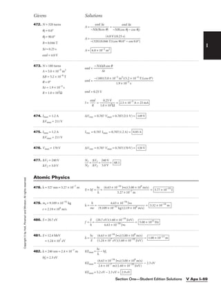
![I
Givens Solutions
Copyright
©
by
Holt,
Rinehart
and
Winston.
All
rights
reserved.
Holt Physics Solution Manual
V Apx I–70
483. hft = 4.1 eV
λ =
h
E
c
= = 3.0 × 10⁻⁷
m = 300 nm
(6.63 × 10⁻³⁴
J•s)(3.00 × 10⁸
m/s)
(4.1 eV)(1.60 × 10⁻¹⁹
eV)
484. l = 2.64 × 10⁻¹⁴
m
mp = 1.67 × 10⁻²⁷
kg
v =
m
h
l
= = 1.50 × 10⁷
m/s
6.63 × 10⁻³⁴
J•s
(1.67 × 10⁻²⁷
kg)(2.64 × 10⁻¹⁴
m)
485. v = 28 m/s
λ = 8.97 × 10−37
m
m =
λ
h
v
= = 26 kg
6.63 × 10⁻³⁴
J•s
(8.97 × 10−37
m)(28 m/s)
486. λ = 430.8 nm
λ = 4.308 × 10⁻⁷
m
E = hf =
h
λ
c
= = 4.62 × 10⁻¹⁹
J
(6.63 × 10⁻³⁴
J•s)(3.00 × 10⁸
m/s)
4.308 × 10⁻⁷
m
487. E = 1.78 eV
f =
E
h
= = 4.30 × 10¹⁴
Hz
(1.78 eV)(1.60 × 10⁻¹⁹
J/eV)
6.63 × 10⁻³⁴
J•s
488. E = 3.1 × 10⁻⁶
eV
λ =
h
E
c
= = 0.40 m
(6.63 × 10⁻³⁴
J•s)(3.00 × 10⁸
m/s)
(3.1 × 10⁻⁶
eV)(1.60 × 10⁻¹⁹
J/eV)
489. f = 6.5 × 10¹⁴
Hz
KEmax = 0.20 eV
ft =
hf − K
h
Emax
ft =
ft = 6.0 × 10¹⁴
Hz
[(6.63 × 10⁻³⁴
J•s)(6.5 × 10¹⁴
Hz) − (0.20 eV)(1.60 × 10⁻¹⁹
J/eV)]
6.63 × 10⁻³⁴
J•s
KEmax =
h
λ
c
− hft
KEmax = − 2.16 eV
KEmax = 2.40 eV − 2.16 eV = 0.24 eV
(6.63 × 10⁻³⁴
J•s)(3.00 × 10⁸
m/s)
(5.19 × 10⁻⁷
m)(1.60 × 10⁻¹⁹
J/eV)
490. λ = 519 nm = 5.19 × 10⁻⁷
m
hft = 2.16 eV
491. v = 5.6 × 10⁻⁶
m/s
λ = 2.96 × 10⁻⁸
m
m =
λ
h
v
= = 4.0 × 10⁻²¹
kg
6.63 × 10⁻³⁴
J•s
(2.96 × 10⁻⁸
m)(5.6 × 10⁻⁶
m/s)
492. ft = 1.36 × 10¹⁵
Hz
hft = = 5.64 eV
(6.63 × 10⁻³⁴
J•s)(1.36 × 10¹⁵
Hz)
1.60 × 10⁻¹⁹
J/eV
493. m = 7.6 × 10⁷
kg
v = 35 m/s
λ =
m
h
v
= = 2.5 × 10−43
m
6.63 × 10⁻³⁴
J•s
(7.6 × 10⁷
kg)(35 m/s)
494. hft = 5.0 eV
λ =
h
E
c
= = 2.5 × 10⁻⁷
m = 250 nm
(6.63 × 10⁻³⁴
J•s)(3.00 × 10⁸
m/s)
(5.0 eV)(1.60 × 10⁻¹⁹
eV)](https://image.slidesharecdn.com/physicssolutions-230306125240-7bc050a7/85/physics-solutions-pdf-323-320.jpg)

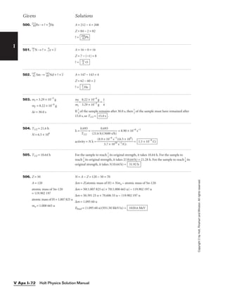


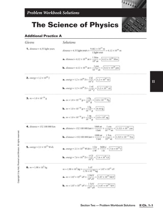
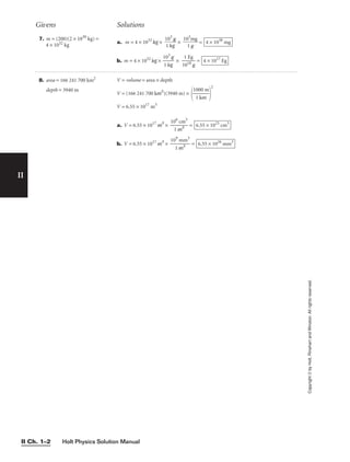
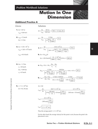


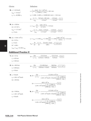
![Section Two — Problem Workbook Solutions II Ch. 2–5
II
Copyright
©
by
Holt,
Rinehart
and
Winston.
All
rights
reserved. 4. vi = vavg = 518 km/h
vf = (0.600) vavg
∆t = 2.00 min
vavg =
518
k
h
m
60
1
m
h
in
1
1
0
k
3
m
m
= 8.63 × 10³
m/min
∆x =
1
2
(vi + vf)∆t =
1
2
[vavg + (0.600) vavg]∆t =
1
2
(1.600)(8.63 × 10³
m/min)(2.00 min)
∆x = 13.8 × 10³
m = 13.8 km
Givens Solutions
5. ∆t = 30.0 s
vi = 30.0 km/h
vf = 42.0 km/h
∆x =
1
2
(vi + vf)∆t =
1
2
(30.0 km/h + 42.0 km/h)
36
1
0
h
0 s
(30.0 s)
∆x =
1
2
72.0
k
h
m
36
1
0
h
0 s
(30.0 s)
∆x = 3.00 × 10⁻¹
km = 3.00 × 10²
m
1. vi = 186 km/h
vf = 0 km/h = 0 m/s
a = −1.5 m/s2
∆t =
vf −
a
vi
= =
−
−
5
1
1
.5
.7
m
m
/s
/
2
s
= 34 s
0 m/s − (186 km/h)
36
1
0
h
0 s
1
1
0
k
3
m
m
−1.5 m/s2
Additional Practice D
6. vf = 96 km/h
vi = 0 km/h
∆t = 3.07 s
∆x =
1
2
(vi + vf)∆t =
1
2
(0 km/h + 96 km/h)
36
1
0
h
0 s
1
1
0
k
3
m
m
(3.07 s)
∆x =
1
2
96 × 103
m
h
(8.53 + × 10−4
h) = 41 m
7. ∆x = 290.0 m
∆t = 10.0 s
vf = 0 km/h = 0 m/s
vi =
2
∆
∆
t
x
− vf =
(2)(
1
2
0
9
.
0
0
.0
s
m)
− 0 m/s =
(Speed was in excess of 209 km/h.)
58.0 m/s = 209 km/h
8. ∆x = 5.7 × 10³
km
∆t = 86 h
vf = vi + (0.10) vi
vf + vi =
2
∆
∆
t
x
vi (1.00 + 0.10) + vi =
2
∆
∆
t
x
vi =
(2)
(
(
2
5
.
.
1
7
0
×
)(
1
8
0
6
3
h
k
)
m)
= 63 km/h
9. vi = 2.60 m/s
vf = 2.20 m/s
∆t = 9.00 min
∆x =
1
2
(vi + vf)∆t =
1
2
(2.60 m/s + 2.20 m/s)(9.00 min)
m
60
in
s
=
1
2
(4.80 m/s)(5.40 × 102
s)
∆x = 1.30 × 10³
m = 1.30 km
2. vi = −15.0 m/s
vf = 0 m/s
a = +2.5 m/s2
vi = 0 m/s
vf = +15.0 m/s
a = +2.5 m/s
For stopping:
∆t1 =
vf
a
− vi
=
0 m/s
2
−
.5
(−
m
1
/
5
s
.
2
0 m/s)
=
1
2
5
.5
.0
m
m
/s
/
2
s
= 6.0 s
For moving forward:
∆t2 =
vf
a
− vi
= =
1
2
5
.5
.0
m
m
/s
/
2
s
= 6.0 s
∆ttot = ∆t1 + ∆t2 = 6.0 s + 6.0 s = 12.0 s
15.0 m/s − 0.0 m/s
2.5 m/s2](https://image.slidesharecdn.com/physicssolutions-230306125240-7bc050a7/85/physics-solutions-pdf-336-320.jpg)

![Section Two — Problem Workbook Solutions II Ch. 2–7
II
Copyright
©
by
Holt,
Rinehart
and
Winston.
All
rights
reserved.
10. vi = 24.0 m/s
a = −0.850 m/s2
∆t = 28.0 s
vf = vi + a∆t = 24.0 m/s + (− 0.850 m/s2
)(28.0 s) = 24.0 m/s − 23.8 m/s = +0.2 m/s
Givens Solutions
11. a = +2.67 m/s2
∆t = 15.0 s
∆x = +6.00 × 10²
m
vi ∆t = ∆x −
1
2
a∆t2
vi =
∆
∆
x
t
−
1
2
a∆t =
6.00
15
×
.0
10
s
2
m
−
1
2
(2.67 m/s2
)(15.0 s) = 40.0 m/s − 20.0 m/s = +20.0 m/s
12. a = 7.20 m/s2
∆t = 25.0 s
vf = 3.00 × 10²
ms
vi = vf − a∆t
vi =(3.00 × 10²
m/s) − (7.20 m/s2
)(25.0 s) = (3.00 × 10²
m/s) − (1.80 × 10²
m/s)
vi = 1.20 × 10²
m/s
13. vi = 0 m/s
∆x = 1.00 × 10²
m
∆t = 12.11 s
∆x = vi∆t +
1
2
a∆t2
Because vi = 0 m/s,
a =
2
∆
∆
t2
x
=
(2)(
(
1
1
.0
2
0
.1
×
1
1
s)
0
2
2
m)
= 1.36 m/s2
8. vi = 0 m/s
vf = 3.06 m/s
a = 0.800 m/s2
∆t2 = 5.00 s
∆t1 =
vf
a
− vi
=
3.0
0
6
.
m
80
/
0
s
m
−
/
0
s2
m/s
= 3.82
∆x1 = vi∆t1 +
1
2
a∆t1
2
= (0 m/s) (3.82 s) +
1
2
(0.800 m/s2
) (3.82 s)2
= 5.84 m
∆x2 = vf∆t2 = (3.06 m/s)(5.00 s) = 15.3 m
∆xtot = ∆x1 + ∆x2 = 5.84 m + 15.3 m = 21.1 m
9. vf = 3.50 × 10²
km/h
vi = 0 km/h = 0 m/s
a = 4.00 m/s2
∆t =
(vf
a
− vi)
= =
∆x = vi∆t +
1
2
a∆t2
= (0 m/s)(24.3 s) +
1
2
(4.00 m/s2
)(24.3 s)2
∆x = 1.18 × 10³
m = 1.18 km
24.3 s
(3.50 × 10²
km/h − 0 km/h)
36
1
0
h
0 s
1
1
0
k
3
m
m
(4.00 m/s2)
14. vi = 3.00 m/s
∆x = 1.00 × 10²
m
∆t = 12.11 s
a =
2(∆x
∆
−
t2
vi∆t)
=
a =
a =
(
(
2
1
)
2
(
.
6
1
4
1
m
s)2
)
= 0.87 m/s2
(2)(1.00 × 10²
m − 36.3 m)
(12.11 s)2
(2)[1.00 × 10²
m − (3.00 m/s)(12.11 s)]
(12.11 s)2
15. vf = 30.0 m/s
vi = 18.0 m/s
∆t = 8.0 s
a =
vf
∆
−
t
vi
= =
12
8
.0
.0
m
s
/s
= 1.5 m/s2
30.0 m/s − 18.0 m/s
8.0 s](https://image.slidesharecdn.com/physicssolutions-230306125240-7bc050a7/85/physics-solutions-pdf-338-320.jpg)
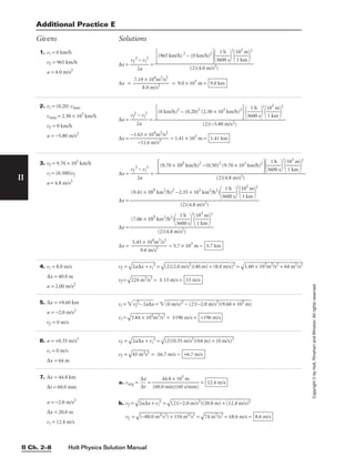


![Section Two — Problem Workbook Solutions II Ch. 3–1
Two-Dimensional
Motion and Vectors
Problem Workbook Solutions
II
Copyright
©
by
Holt,
Rinehart
and
Winston.
All
rights
reserved.
1. ∆tx = 7.95 s
∆y = 161 m
d = 226 m
d2
= ∆x2
+ ∆y2
∆x =
d
2
−
∆
y
2
=
(2
26
m
)2
−
(
16
1
m
)2
=
5.
11
×
1
04
m
2
−
2
.5
9
×
1
04
m
2
∆x =
2.
52
×
1
04
m
2
= 159 m
∆x =
v =
∆
∆
t
x
x
=
1
7
5
.9
9
5
m
s
= 20.0 m/s
159 m
Additional Practice A
Givens Solutions
2. d1 = 5.0 km
θ1 = 11.5°
d2
= 1.0 km
q2 = −90.0°
∆xtot = d1(cos q1) + d2(cos q2) = (5.0 km)(cos 11.5°) + (1.0 km)[cos(−90.0°)]
∆xtot = 4.9 km
∆ytot = d1(sin q1) + d2(sin q2) = (5.0 km)(sin 11.5°) + (1.0 km)[sin(−90.0°
)]
= 1.0 km − 1.0 km
∆ytot = 0.0 km
d =
(∆
xt
ot
)2
+
(
∆
yt
ot
)2
=
(4
.9
k
m
)2
+
(
0.
0
km
)2
d =
q = tan−1
∆
∆
x
yt
t
o
o
t
t
= tan−1
0
4
.
.
0
9
k
k
m
m
= 0.0°
, or due east
4.9 km
3. ∆x = 5 jumps
1 jump = 8.0 m
d = 68 m
d2
= ∆x2
+ ∆y2
∆y =
d
2
−
∆
x
2
=
(6
8
m
)2
−
[
(5
)(
8.
0
m
)]
2
=
4.
6
×
1
03
m
2
−
1
.6
×
1
03
m
2
∆y =
3.
0
×
1
03
m
= 55 m
number of jumps northward =
8.0
5
m
5
/
m
jump
= 6.9 jumps =
q = tan−1
∆
∆
x
y
= tan−1
(5)
5
(
5
8.
m
0 m)
= 36° west of north
7 jumps
4. ∆x = 25.2 km
∆y = 21.3 km
d =
∆
x
2
+
∆
y
2
=
(2
5.
2
km
)2
+
(
21
.3
k
m
)2
d =
63
5
km
2
+
4
54
k
m
2
=
10
89
k
m
2
d =
q = tan−1
∆
∆
x
y
= tan−1
2
2
1
5
.
.
3
2
k
k
m
m
q = 42.6° south of east
33.00 km](https://image.slidesharecdn.com/physicssolutions-230306125240-7bc050a7/85/physics-solutions-pdf-342-320.jpg)
![Holt Physics Solution Manual
II Ch. 3–4
II
Copyright
©
by
Holt,
Rinehart
and
Winston.
All
rights
reserved.
2. v = 3.53 × 10³
km/h
∆t1 = 20.0 s
∆t2 = 10.0 s
q1 = 15.0°
q2 = 35.0°
∆x1 = v∆t1(cos q1)
∆x1 = (3.53 × 10³
km/h)
36
1
0
h
0 s
(103
m/km)(20.0 s)(cos 15.0°) = 1.89 × 10⁴
m
∆y1 = v∆t1(sin q1)
∆y1 = (3.53 × 10³
km/h)
36
1
0
h
0 s
(103
m/km)(20.0 s)(sin 15.0°) = 5.08 × 10³
m
∆x2 = v∆t2(cos q2)
∆x2 = (3.53 × 10³
km/h)
36
1
0
h
0 s
(103
m/km)(10.0 s)(cos 35.0°) = 8.03 × 10³
m
∆y2 = v∆t2(sin q2)
∆y2 = (3.53 × 10³
km/h)
36
1
0
h
0 s
(103
m/km)(10.0 s)(sin 35.0°) = 5.62 × 10³
m
∆ytot = ∆y1 + ∆y2 = 5.08 × 10³
m + 5.62 × 10³
m =
∆xtot = ∆x1 + ∆x2 = 1.89 × 10⁴
m + 8.03 × 10³
m =
d =
(∆
xt
ot
)2
+
(
∆
yt
ot
)2
=
(2
.6
9
×
1
04
m
)2
+
(
1.
07
×
1
04
m
)2
d =
7.
24
×
1
08
m
2
+
1
.1
1
×
1
08
m
2
=
8.
35
×
1
08
m
d =
q = tan−1
∆
∆
x
yt
t
o
o
t
t
= tan−1
1
2
.
.
0
6
7
9
×
×
1
1
0
0
4
4
m
m
q = 21.7° above the horizontal
2.89 × 10⁴
m
2.69 × 10⁴
m
1.07 × 10⁴
m
Givens Solutions
3. ∆x1 + ∆x2 = 2.00 × 10²
m
∆y1 + ∆y2 = 0
q1 = 30.0°
q2 = −45.0°
v = 11.6 km/h
∆y1 = d1(sin q1) = −∆y2 = −d2(sin q2)
d1 = −d2
s
s
i
i
n
n
q
q
2
1
= −d2
si
s
n
i
(
n
−
3
4
0
5
.
.
0
0
°
°)
= 1.41d2
∆x1 = d1(cos q1) = (1.41d2)(cos 30.0°) = 1.22d2
∆x2 = d2(cos q2) = d2[cos(−45.0°)] = 0.707d2
∆x1 + ∆x2 = d2(1.22 + 0.707) = 1.93d2 = 2.00 × 10²
m
d2 =
d1 = (1.41)d2 = (1.41)(104 m) =
v = 11.6 km/h = (11.6 km/h)
36
1
0
h
0 s
(103
m/km) = 3.22 m/s
∆t1 =
d
v
1
=
3
1
.2
4
2
7
m
m
/s
= 45.7 s
∆t2 =
d
v
2
=
3
1
.2
0
2
4
m
m
/s
= 32.3 s
∆ttot = ∆t1 + ∆t2 = 45.7 s + 32.3 s = 78.0 s
147 m
104 m](https://image.slidesharecdn.com/physicssolutions-230306125240-7bc050a7/85/physics-solutions-pdf-345-320.jpg)


![Holt Physics Solution Manual
II Ch. 4–2
Givens Solutions
II
Copyright
©
by
Holt,
Rinehart
and
Winston.
All
rights
reserved.
2. mb = 253 kg
mw = 133 kg
g = 9.81 m/s2
Fnet = Fn,1 + Fn,2 − mbg − mwg = 0
The weight of the weightlifter and barbell is distributed equally on both feet, so the
normal force on the first foot (Fn,1) equals the normal force on the second foot (Fn,2).
2Fn,1 = (mb + mw)g = 2Fn,2
Fn,1 = Fn,2 =
(mb +
2
mb)g
=
Fn,1 = Fn,2 = = 1.89 × 10³
N
Fn,1 = Fn,2 = 1.89 × 10³
N upward on each foot
(386 kg)(9.81 m/s2
)
2
(253 kg + 33 kg)
9.81
m
s2
2
3. Fdown = 1.70 N
Fnet = 4.90 N
Fnet
2
= Fforward
2
+ Fdown
2
Fforward =
F
ne
t
2
−
F
do
w
n
2
=
(4
.9
0
N
)2
−
(
1.
70
N
)2
Fforward =
21
.1
N
2
= 4.59 N
4. m = 3.10 × 10²
kg
g = 9.81 m/s2
q1 = 30.0°
q2 = − 30.0°
Fx,net = ΣFx = FT,1(sin q1) + FT,2(sin q2) = 0
Fy,net = ΣFy = FT,1(cos q1) + FT,2(cos q2) + Fg = 0
FT,1(sin 30.0°) = −FT,2[sin (−30.0°)]
FT,1 = FT,2
FT,1(cos q1) + FT,1(cos q2) = −Fg = mg
FT,1(cos 30.0°) + FT,1[cos (−30.0°)] = (3.10 × 10²
kg)(9.81 m/s2
)
FT,1 =
FT,1 = FT,2 =
As the angles q1 and q2 become larger, cos q1 and cos q2 become smaller. Therefore,
FT,1 and FT,2 must become larger in magnitude.
1.76 × 10³
N
(3.10 × 10²
kg)(9.81 m/s2
)
(2)(cos 30.0°)[cos(−30.0°)]](https://image.slidesharecdn.com/physicssolutions-230306125240-7bc050a7/85/physics-solutions-pdf-353-320.jpg)
![Section Two — Problem Workbook Solutions II Ch. 4–3
II
Copyright
©
by
Holt,
Rinehart
and
Winston.
All
rights
reserved.
Givens Solutions
5. m = 155 kg
FT,1 = 2FT,2
g = 9.81 m/s2
q1 = 90° − q2
Fx,net = FT,1(cos q1) − FT,2(cos q2) = 0
Fy,net = FT,1(sin q1) + FT,2(sin q2) − mg = 0
FT,1[(cos q1) −
1
2
(cos q2)] = 0
2 (cos q1) = cos q2 = cos(90° − q1) = sin q1
2 = tan q1
q1 = tan−1
(2) = 63°
q2 = 90° − 63° = 27°
FT,1(sin q1) +
FT
2
,1
(sin q2) = mg
FT,1 =
FT,1 = =
(155
0
k
.8
g
9
)(
+
9.
0
8
.
1
2
m
3
/s2
)
=
(155 kg
1
)
.1
(9
2
.81 m)
FT,1 =
FT,2 = 6.80 × 10²
N
1.36 × 1.36 × 103
N
(155 kg)(9.81 m/s2
)
(sin 63°) +
(sin
2
27°)
mg
(sin θ1) +
1
2
(sin θ2)
1. vi = 173 km/h
vf = 0 km/h
∆x = 0.660 m
m = 70.0 kg
g = 9.81 m/s2
a =
vf
2
2∆
−
x
vi
2
=
a = −1.75 × 10³
m/s2
F = ma = (70.0 kg)(−1.75 × 10³
m/s2
) =
Fg = mg = (70.0 kg)(9.81 m/s2
) =
The force of deceleration is nearly 178 times as large as David Purley’s weight.
6.87 × 10²
N
−1.22° × 105
N
[(0 km/h)2
− (173 km/h)2
](103
m/km)2
(1 h/3600 s)2
(2)(0.660 m)
2. m = 2.232 × 10⁶
kg
g = 9.81 m/s2
anet = 0 m/s2
a. Fnet = manet = Fup − mg
Fup = manet + mg = m(anet + g) = (2.232 × 10⁶
kg)(0 m/s2
+ 9.81 m/s2
)
Fup = = mg
b. Fdown = mg(sin q)
anet =
F
m
net
=
Fup −
m
Fdown
=
mg − m
m
g(sin q)
anet = g(1 − sin q) = (9.81 m/s2
)[1.00 − (sin 30.0°)] =
9.81
2
m/s2
= 4.90 m/s2
anet = 4.90 m/s2
up the incline
2.19 × 10⁷
N
3. m = 40.00 mg
= 4.00 × 10⁻⁵
kg
g = 9.807 m/s2
anet = (400.0)g
Fnet = Fbeetle − Fg = manet = m(400.0) g
Fbeetle = Fnet + Fg = m(400.0 + 1)g = m(401)g
Fbeetle = (4.000 × 10⁻⁵
kg)(9.807 m/s2
)(401) =
Fnet = Fbeetle − Fg = m(400.0) g = (4.000 × 10⁻⁵
kg)(9.807 m/s2
)(400.0)
Fnet =
The effect of gravity is negligible.
1.569 × 10⁻¹
N
1.573 × 10⁻¹
N
Additional Practice C](https://image.slidesharecdn.com/physicssolutions-230306125240-7bc050a7/85/physics-solutions-pdf-354-320.jpg)
![Holt Physics Solution Manual
II Ch. 4–6
II
Copyright
©
by
Holt,
Rinehart
and
Winston.
All
rights
reserved.
13. m = 409 kg
d = 6.00 m
q = 30.0°
g = 9.81 m/s2
Fapplied = 2080 N
vi = 0 m/s
a. Fnet = Fapplied − mg(sin q) = 2080 N − (409 kg)(9.81 m/s2
)(sin 30.0°)
Fnet = 2080 N − 2010 N = 70 N
Fnet =
b. anet =
F
m
net
=
4
7
0
0
9
N
kg
= 0.2 m/s2
anet =
c. d = vi∆t +
1
2
anet ∆t2
= (0 m/s)∆t +
1
2
(0.2 m/s2
)∆t2
∆t =
(
(
2
0
)
.
(
2
6
.
m
0
0
/s
m
2
)
)
= 8 s
0.2 m/s2
at 30.0° above the horizontal
70 N at 30.0° above the horizontal
vf =
2a
ne
t∆
y
+
v
i
2
=
(2
)(
1.
40
m
/s
2
)
(2
5.
0
m
)
+
(
0
m
/s
)2
vf = 8.37 m/s
Givens Solutions
14. amax = 0.25 m/s2
Fmax = 57 N
Fapp = 24 N
a. m =
F
am
m
a
a
x
x
=
0.2
5
5
7
m
N
/s2
=
b. Fnet = Fmax − Fapp = 57 N − 24 N = 33 N
anet =
F
m
net
=
2.3
3
×
3
1
N
02
kg
= 0.14 m/s2
2.3 × 10²
kg
15. m = 2.55 × 10³
kg
FT = 7.56 × 10³
N
qT = −72.3°
Fbuoyant = 3.10 × 10⁴
N
Fwind = −920 N
g = 9.81 m/s2
∆y = −45.0 m
vi = 0 m/s
a. Fx,net = ΣFx = max,net = FT(cos qT) + Fwind
Fx,net = (7.56 × 10³
N)[cos(−72.3°)] − 920 N = 2.30 × 10³
N − 920 N = 1.38 × 10³
N
Fy,net = ΣFy = may,net = FT(sin qT) + Fbuoyant + Fg = FT(sin qT) + Fbuoyant − mg
Fy,net = (7.56 × 10³
N)[sin(−72.3°)] = 3.10 × 10⁴
N − (2.55 × 10³
kg)(9.81 m/s2
)
Fy,net = −7.20 × 10³
N + 3.10 × 10⁴
N − 2.50 × 104
= −1.2 × 10³
N
Fnet =
(F
x,
ne
t)
2
+
(
F
y,n
et
)2
=
(1
.3
8
×
1
03
N
)2
+
(
−
1.
2
×
1
03
N
)2
Fnet =
1.
90
×
1
06
N
2
+
1
.4
×
1
06
N
2
Fnet =
3.
3
×
1
06
N
2
= 1.8 × 10³
N
q = tan−1
F
F
x
y,
,
n
n
e
e
t
t
= tan−1
−
1.
1
3
.
8
2
×
×
1
1
0
0
3
3
N
N
q = −41°
Fnet =
b. anet =
F
m
net
=
2
1
.5
.8
5
×
×
1
1
0
0
3
3
N
kg
anet =
c. Because vi = 0
∆y =
1
2
ay,net ∆t2
∆x =
1
2
ax,net ∆t2
∆x =
a
a
x
y,
,
n
n
e
e
t
t
∆y = ∆y =
ta
∆
n
y
q
∆x =
ta
−
n
4
(
5
−
.0
41
m
°)
= 52 m
anet(cos q)
anet(sin q)
0.71 m/s2
1.8 × 10³
N at 41° below the horizontal](https://image.slidesharecdn.com/physicssolutions-230306125240-7bc050a7/85/physics-solutions-pdf-357-320.jpg)
![Section Two — Problem Workbook Solutions II Ch. 4–7
II
Copyright
©
by
Holt,
Rinehart
and
Winston.
All
rights
reserved.
1. m = 11.0 kg
mk = 0.39
g = 9.81 m/s2
Additional Practice D
Givens Solutions
2. m = 2.20 × 10⁵
kg
ms = 0.220
g = 9.81 m/s2
Fs,max = msFn = msmg
Fs,max = (0.220)(2.20 × 10⁵
kg)(9.91 m/s2
) = 4.75 × 10⁵
N
3. m = 25.0 kg
Fapplied = 59.0 N
q = 38.0°
ms = 0.599
g = 9.81 m/s2
Fs,max = msFm
Fn = mg(cos q) + Fapplied
Fs,max = ms[mg(cos q) = Fapplied] = (0.599)[(25.0 kg)(9.81 m/s2
)(cos 38.0° + 59.0 N]
Fs,max = (0.599)(193 N + 59 N) = (0.599)(252 N) =
Alternatively,
Fnet = mg(sin q) − Fs,max = 0
Fs,max = mg(sin q) = (25.0 kg)(9.81 m/s2
)(sin 38.0°) = 151 N
151 N
Fk = mkFn = mkmg
Fk = (0.39) (11.0 kg)(9.81 m/s2
) = 42.1 N
4. q = 38.0°
g = 9.81 m/s2
Fnet = mg(sin q) − Fk = 0
Fk = mkFn = mkmg(cos q)
mkmg(cos q) = mg(sin q)
mk =
c
si
o
n
s
q
q
= tan q = tan 38.0°
mk = 0.781
5. q = 5.2°
g = 9.81 m/s2
Fnet = mg(sin q) − Fk = 0
Fk = mkFn = mkmg(cos q)
mkmg(cos q) = mg(sin q)
mk =
c
si
o
n
s
q
q
= tan q = tan 5.2°
mk = 0.091](https://image.slidesharecdn.com/physicssolutions-230306125240-7bc050a7/85/physics-solutions-pdf-358-320.jpg)
![Section Two — Problem Workbook Solutions II Ch. 4–9
II
Copyright
©
by
Holt,
Rinehart
and
Winston.
All
rights
reserved.
1. Fapplied = 130 N
anet = 1.00 m/s2
mk = 0.158
g = 9.81 m/s2
Fnet = manet = Fapplied − Fk
Fk = mkFn = mkmg
manet + mkmg = Fapplied
m(anet + mkg) = Fapplied
m =
an
F
e
a
t
p
+
pli
m
ed
kg
=
m = = = 51 kg
130 N
2.55 m/s2
130 N
1.00 m/s2
+ 1.55 m/s2
130 N
1.00 m/s2
+ (0.158)(9.81 m/s2
)
2. Fnet = −2.00 × 10⁴
N
q = 10.0°
mk = 0.797
g = 9.81 m/s2
Fnet = manet = mg(sin q) − Fk
Fk = mkFn = mkmg(cos q)
m[g(sin q) − mkg(cos q)] = Fnet
m =
g[sin q −
Fn
m
e
k
t
(cos q)]
=
m = =
(9.8
−
1
2.
m
00
/s
×
2
)
1
(−
04
0.
N
611)
m =
Fn = mg(cos q) = (3.34 × 10³
kg)(9.81 m/s2
)(cos 10.0°) = 3.23 × 10⁴
N
3.34 × 10³
kg
−2.00 × 10⁴
N
(9.81 m/s2
)(0.174 − 0.785)
−2.00 × 10⁴
N
(9.81 m/s2
)[(sin 10.0°) − (0.797)(cos 10.0°)]
3. Fnet = 6.99 × 10³
N
q = 45.0°
mk = 0.597
Fnet = manet = mg(sin q) − Fk
Fk = mkFn = mkmg(cos q)
m[g(sin q) − mkg(cos q)] = Fnet
m =
g[sin q −
Fn
m
e
k
t
(cos q)]
=
m = =
(9.8
6
1
.9
m
9
/
×
s2
1
)
0
(
3
0.
N
285)
m =
Fn = mg(cos q) = (2.50 × 10³
kg)(9.81 m/s2
)(cos 45.0°) = 1.73 × 10⁴
N
2.50 × 10³
kg
6.99 × 10³
N
(9.81 m/s2
)(0.707 − 0.422)
6.99 × 10³
N
(9.81 m/s2
)[(sin 45.0°) − (0.597)(cos 45.0°)]
4. m = 9.50 kg
q = 30.0 °
Fapplied = 80.0 N
anet = 1.64 m/s2
g = 9.81 m/s2
Fnet = manet = Fapplied − Fk − mg(sin q)
Fk = mkFn = mkmg(cos q)
mkmg(cos q) = Fapplied − manet − mg(sin q)
mk =
mk =
80.0 N − (9.50 kg)[1.64 m/s2
+ (9.81 m/s2
)(sin 30.0°)]
(9.50 kg)(9.81 m/s2
)(cos 30.0°)
Fapplied − m[anet + g (sin q)]
mg(cos q)
Additional Practice E
Givens Solutions](https://image.slidesharecdn.com/physicssolutions-230306125240-7bc050a7/85/physics-solutions-pdf-360-320.jpg)
![II
Givens Solutions
Copyright
©
by
Holt,
Rinehart
and
Winston.
All
rights
reserved.
Holt Physics Solution Manual
II Ch. 4–10
6. q = 38.0°
mk = 0.100
g = 9.81 m/s2
Fnet = manet = mg(sin q) − Fk
Fk = mkFn = mkmg(cos q)
manet = mg[sin q − mk(cos q)]
anet = g[sin q − mk(cos q)] = (9.81 m/s2
)[(sin 38.0°) − (0.100)(cos 38.0°)]
anet = (9.81 m/s2
)(0.616 − 7.88 × 10⁻²
) = (9.81 m/s2
)(0.537)
anet =
Acceleration is independent of the rider’s and sled’s masses. (Masses cancel.)
5.27 m/s2
mk = =
mk = =
mk = 0.222
17.9 N
(9.50 kg)(9.81 m/s2
)(cos 30.0°)
80.0 N − 62.1 N
(9.50 kg)(9.81 m/s2
)(cos 30.0°)
80.0 N − (9.50 kg)(6.54 m/s2
)
(9.50 kg)(9.81 m/s2
)(cos 30.0°)
80.0 N − (9.50 kg)[1.64 m/s2
+ 4.90 m/s2
)
(9.50 kg)(9.81 m/s2
)(cos 30.0°)
5. m = 1.89 × 10⁵
kg
Fapplied = 7.6 × 10⁵
N
anet = 0.11 m/s2
Fnet = manet = Fapplied − Fk
Fk = Fapplied − manet = 7.6 × 10⁵
N − (1.89 × 10⁵
)(0.11 m/s2
) = 7.6 × 10⁵
N − 2.1 × 10⁴
N
Fk = 7.4 × 10⁵
N
7. ∆t = 6.60 s
q = 34.0°
mk = 0.198
g = 9.81 m/s2
vi = 0 m/s
Fnet = manet = mg(sin q) − Fk
Fk = mkFn = mkmg(cos q)
manet = mg[sin q − mk(cos q)]
anet = g[sin q − mk(cos q)] = (9.81 m/s2
)[(sin 34.0°) − (0.198)(cos 34.0°)]
anet = (9.81 m/s2
)(0.559 − 0.164) = (9.81 m/s2
)(0.395)
anet =
vf = vi + anet∆t = 0 m/s + (3.87 m/s2
)(6.60 s)
vf = 25.5 m/s2
= 92.0 km/h
3.87 m/s2](https://image.slidesharecdn.com/physicssolutions-230306125240-7bc050a7/85/physics-solutions-pdf-361-320.jpg)

![Holt Physics Solution Manual
II Ch. 5–2
II
5. d = 5.45 m
W = 4.60 × 10⁴
J
q = 0°
Fnet = Flift − Fg = 0
F = Flift = Fg
W = Fd(cos q) = Fgd(cos q)
Fg =
d(c
W
os q)
=
(5.
4
4
.
5
60
m
×
)(
1
c
0
o
4
s
J
0°)
= 8.44 103
N
Givens Solutions
Copyright
©
by
Holt,
Rinehart
and
Winston.
All
rights
reserved.
6. d = 52.0 m
m = 40.0 kg
W = 2.04 × 10⁴
J
q = 0°
F =
d(c
W
os q)
=
(5
2
2
.
.
0
0
4
m
×
)
1
(c
0
o
4
s
J
0°)
= 392 N
7. d = 646 m
W = 2.15 × 10⁵
J
q = 0°
F =
d(c
W
os q)
=
(64
2
6
.1
m
5 ×
)(
1
co
0
s
5
0
J
°)
= 333 N
8. m = 1.02 × 10³
kg
d = 18.0 m
angle of incline = q = 10.0°
q′ = 0°
g = 9.81 m/s2
mk = 0.13
Fnet = Fg − Fk = mg (sin q) − mkmg(cos q)
Wnet = Fnetd(cos q′) = mgd(cos q′)[(sin q) − mk(cos q)]
Wnet = (1.02 × 10³
kg)(9.81 m/s2
)(18.0 m)(cos 0°)[(sin 10.0°) − (0.13)(cos 10.0°)]
Wnet = (1.02 × 10³
kg)(9.81 m/s2
)(18.0 m)(0.174 − 0.128)
Wnet = (1.02 × 10³
kg)(9.81 m/s2
)(18.0 m)(0.046)
Wnet = 8.3 × 10³
J
9. d = 881.0 m
Fapplied = 40.00 N
q = 45.00°
Fk = 28.00 N
q′ = 0°
Wnet = Fnetd(cos q′)
Fnet = Fapplied(cos q) − Fk
Wnet = [Fapplied(cos q) − Fk]d(cos q′)
Wnet = [40.00 N(cos 45.00°) − 28.00° N](881.0 m)(cos q)
Wnet = (28.28 N − 28.00 N)(881.0 m) = (0.28 N)(881.0 m)
Wnet = 246.7 J
10. m = 9.7 × 10³
kg
q = 45°
F = F1 = F2 = 1.2 × 10³
N
d = 12 m
Wnet = Fnetd(cos q) = (F1 + F2)d(cos q) = 2Fd(cos q)
Wnet = (2)(1.2 × 10³
N)(12 m)(cos 45°) = 2.0 × 10⁴
J
11. m = 1.24 × 10³
kg
F1 = 8.00 × 10³
N east
F2 = 5.00 × 10³
N 30.0°
south of east
d = 20.0 m south
Only F2 contributes to the work done in moving the flag south.
q = 90.0° − 30.0° = 60.0°
Wnet = Fnetd(cos q) = F2d(cos q) = (5.00 × 10³
N)(20.0 m)(cos 60.0°)
Wnet = 5.00 × 10⁴
J](https://image.slidesharecdn.com/physicssolutions-230306125240-7bc050a7/85/physics-solutions-pdf-363-320.jpg)
![Section Two — Problem Workbook Solutions II Ch. 5–3
II
1. ∆x = 1.00 × 10²
m
∆t = 9.85 s
KE = 3.40 × 10³
J
v =
∆
∆t
x
KE =
1
2
mv2
=
1
2
m
∆
∆
x
t
2
m =
2K
∆
E
x
∆
2
t2
= = 66.0 kg
(2)(3.40 × 10³
J)(9.85 s)2
(1.00 × 10²
m)2
Additional Practice B
Givens Solutions
Copyright
©
by
Holt,
Rinehart
and
Winston.
All
rights
reserved.
2. v = 4.00 × 10²
km/h
KE = 2.10 × 10⁷
J
m =
2
v
K
2
E
= = 3.40 × 10³
kg
(2)(2.10 × 10⁷
J)
(4.00 × 10²
km/h)2
(103
m km)2
(1 h/3600 s)2
3. v = 50.3 km/h
KE = 6.54 × 10³
J
m =
2
v
K
2
E
= = 67.0 kg
(2)(6.54 × 10³
J)
(50.3 km/h)2
(103
m/km)2
(1 h/3600 s)
4. v = 318 km/h
KE = 3.80 MJ
m =
2
v
K
2
E
= = 974 kg
(2)(3.80 × 10⁶
J)
(318 km/h)2
(103
m/km)2
(1 h/3600 s)
5. m = 51.0 kg
KE = 9.96 × 10⁴
J
v =
2
m
K
E
=
(2
)(
9
5
.
9
1
6
.
0
×
kg
10
4
J)
= 62.5 m/s = 225 km/h
6. ∆x = 93.625 km
∆t = 24.00 h
m = 55 kg
a. vavg =
∆
∆
x
t
=
(24
9
.
.
0
3
0
62
h
5
)(
×
3
1
6
0
0
4
0
m
s/h)
=
b. KE =
1
2
mv2
=
1
2
(55 kg)(1.084 m/s)2
= 32 J
1.084 m/s
7. m = 3.38 × 1031
kg
KE = 1.10 × 1042
J
v =
2
m
K
E
=
(2
3
)
.
(
3
1
8
.1
×
0
1
×
0
1
3
1
0
4
k
2
g
J
)
= 2.55 × 10⁵
m/s = 255 km/s
8. m = 680 kg
v = 56.0 km/h
KELB = 3.40 × 10³
J
a. KE =
1
2
mv2
=
1
2
(680 kg)[(56.0 km/h)(103
m/km)(1 h/3600 s)]2
= 8.23 × 10⁴
J
b.
K
K
E
E
L
p
B
b
=
3
8
.
.
4
2
0
×
×
1
1
0
0
4
3
J
J
=
2
1
4
9. v = 11.2 km/s
m = 2.3 × 10⁵
kg
KE =
1
2
mv2
=
1
2
(2.3 × 10⁵
kg)(11.2 × 10³
m/s)2
= 1.4 × 10¹³
J](https://image.slidesharecdn.com/physicssolutions-230306125240-7bc050a7/85/physics-solutions-pdf-364-320.jpg)
![Holt Physics Solution Manual
II Ch. 5–4
II
Additional Practice C
Givens Solutions
Copyright
©
by
Holt,
Rinehart
and
Winston.
All
rights
reserved.
1. d = 227 m
m = 655 g
g = 9.81 m/s2
Fresistance = (0.0220)mg
q = 0°
KEi = 0 J
Wnet = ∆KE = KEf − KEi = KEf
Wnet = Fnetd(cos q)
Fnet = Fg − Fresistance = mg − (0.0220)mg = mg(1 − 0.0220)
KEf = mg(1 − 0.0220)d(cos q) = (655 × 10−3
kg)(9.81 m/s2
)(1 − 0.0220)(227 m)(cos 0°)
KEf = (0.655 kg)(9.81 m/s2
)(0.9780)(227 m)
KEf = 1.43 × 10³
J
2. vi = 12.92 m/s
Wnet = −2830 J
m = 55.0 kg
Wnet is the work done by friction.
Wnet = ∆KE = KEf − KEi = KEf −
1
2
mvi
2
KEf = Wnet +
1
2
mvi
2
= − 2830 J +
1
2
(55.0 kg)(12.92 m/s)2
= −2830 J + 4590 J
KEf = 1.76 × 10³
J
3. m = 25.0 g
hi = 553 m
hf = 353 m
vi = 0 m/s
vf = 30.0 m/s
g = 9.81 m/s2
q = 0°
Wnet = ∆KE = KEf − KEi =
1
2
mvf
2
−
1
2
mvi
2
Wnet = Fnetd(cos q)
Fnet = Fg − Fr = mg − Fr
d = hi − hf
Wnet = (mg − Fr)(hi − hf)(cos q)
mg − Fr =
1
2
m (vf
2
− vi
2
)
(hi – hf)(cos q)
Fr = m
g −
2(h
(
i
v
−
f
2
h
−
f)(
v
c
i
2
o
)
s q)
= (25.0 × 10⁻³
kg)
9.81 m/s2
−
Fr = (25.0 × 10⁻³
kg)
9.81 m/s2
−
(
9
2
.
)
0
(
0
2.
×
00
10
×
2
1
m
02
2
/
m
s2
)
Fr = (25.0 × 10⁻³
kg)(9.81 m/s2
− 2.25 m/s2
) = (25.0 × 10⁻³
kg)(7.56 m/s2
)
Fr = 0.189 N
(30.0 m/s)2
− (0 m/s)2
(2)(553 m − 353 m)(cos 0°)
4. vi = 404 km/h
Wnet = −3.00 MJ
m = 1.00 × 10³
kg
Wnet = ∆KE = KEf − KEi =
1
2
mvf
2
−
1
2
mvi
2
1
2
mvf
2
=
1
2
mvi
2
+ Wnet
vf = vi
2
+
2
W
m
ne
t
= [(
40
4
km
/h
)(
10
3
m
/k
m
)(
1
h
/3
60
0
s)
]2
+
(
2)
1
(
.
−
0
0
3.
0
×
0
1
×
0
3
1
k
0
g
6
J)
vf =
1.
26
×
1
04
m
2
/
s2
−
6
.0
0
×
1
03
m
2
/
s2
=
6.
6
×
1
03
m
2
/
s2
vf = 81 m/s = 290 km/h
5. m = 45.0 g
hi = 8848.0 m
hf = 8806.0 m
vi = 0 m/s
vf = 27.0 m/s
g = 9.81 m/s2
q = 0°
Wnet = ∆KE = KEf − KEi =
1
2
mvf
2
−
1
2
mvi
2
Wnet = Fnetd(cos q)
Fnet = Fg − Fr = mg − Fr
d = hi − hf
Wnet = mg(hi − hf)(cos q) − Fr(hi − hf)(cos q)
− Fr(hi − hf)(cos q) = Fr(hi − hf)(cos 180° + q) = Wr
1
2
m(vf
2
− vi
2
) = mg(hi − hf)(cos q) + Wr](https://image.slidesharecdn.com/physicssolutions-230306125240-7bc050a7/85/physics-solutions-pdf-365-320.jpg)
![Section Two — Problem Workbook Solutions II Ch. 5–5
II
6. vf = 35.0 m/s
vi = 25.0 m/s
Wnet = 21 kJ
Wnet = ∆KE = KEf − KEi =
1
2
mvf
2
−
1
2
mvi
2
m =
v
2
f
2
W
−
n
v
et
i
2
= =
m =
6.0
4
×
2
1
×
0
1
2
0
m
3
J
2/s2
= 7.0 × 101
kg
42 × 103
J
1220 m2/s2 − 625 m2/s2
(2)(21 × 103
J)
(35.0 m/s)2 − (25.0 m/s)2
Givens Solutions
Copyright
©
by
Holt,
Rinehart
and
Winston.
All
rights
reserved.
7. vi = 104.5 km/h
vf =
1
2
vi
mk = 0.120
g = 9.81 m/s2
q = 180°
Wnet = ∆KE = KEf − KEi =
1
2
mvf
2
−
1
2
mvi
2
Wnet = Wkd(cos q) = Fkd(cos q) = mkmgd(cos q)
1
2
m(vf
2
− vi
2
) = mkmgd(cos q)
d =
2m
v
k
f
g
2
(
−
co
v
s
i
2
q)
=
d = =
d = 268 m
−(3)
1
3
0
.6
4
0
.5
0
m/s
2
−(8)(0.120)(9.81 m/s2
)
1
3
0
.6
4
0
.5
0
m/s
2
1
4
− 1
−(2)(0.120)(9.81 m/s2
)
(2)(0.120)(9.81 m/s2
)(cos 180°)
Additional Practice D
Wr = m[
1
2
(vf
2
− vi
2
) − g(hi − hf)(cos q)] = (45.0 × 10⁻³
kg)
1
2
(27.0 m/s)2
−
1
2
(0 m/s)2
−(9.81 m/s2
)(8848.0 m − 8806.0 m)(cos 0°)
Wr = (45.0 × 10⁻³
kg)[364 m2
/s2
− (9.81 m/s2
)(42.0 m)]
Wr = (45.0 × 10⁻³
kg)(364 m2
/s2
− 412 m2
/s2
)
Wr = (45.0 × 10⁻³
kg)(−48 m2
/s2
) = −2.16 J
1. h = 6.13/2 m = 3.07 m
PEg = 4.80 kJ
g = 9.81 m/s2
m =
P
g
E
h
g
=
(9.81
4.
m
80
/s
×
2)
1
(
0
3
3
.0
J
7 m)
= 1.59 × 10²
kg
2. h = 1.70 m
PEg = 3.04 × 10³
J
g = 9.81 m/s2
m =
P
g
E
h
g
=
(9.81
3.
m
04
/s
×
2
)
1
(
0
1
3
.7
J
0 m)
= 182 kg
3. PEg = 1.48 × 10⁷
J
h = (0.100)(180 km)
g = 9.81 m/s2
m =
P
g
E
h
g
= = 83.8 kg
1.48 × 10⁷
J
(9.81 m/s2
)(0.100)(180 × 103
m)
4. m = 3.6 × 10⁴
kg
PEg = 8.88 × 10⁸
J
g = 9.81 m/s2
h =
P
m
E
g
g
= = 2.5 × 10³
m = 2.5 km
8.88 × 10⁸
J
(3.6 × 10⁴
kg)(9.81 m/s2
)
[(104.5 km/h)(103
m/km)(1 h/3600 s)]2
[
1
2
2
− (1)2
]](https://image.slidesharecdn.com/physicssolutions-230306125240-7bc050a7/85/physics-solutions-pdf-366-320.jpg)

![Section Two — Problem Workbook Solutions II Ch. 5–7
II
10. ∆x = 9.50 × 10²
m
q = 45.0°
m = 65.0 g
g = 9.81 m/s2
x = 55.0 cm
a. vx = vi(cos q) =
∆
∆
x
t
∆t =
vi(c
∆
o
x
s q)
vertical speed of the arrow for the first half of the flight = vi(sin q) = g
∆
2
t
vi(sin q) =
2vi(
g
c
∆
o
x
s q)
vi =
2(
si
n
g
q
∆
)
(
x
c
o
s
q
)
= = 96.5 m/s
KEi =
1
2
mvi
2
=
1
2
(65.0 × 10⁻³
kg)(96.5 m/s)2
=
b. From the conservation of energy,
PEelastic = KEi
1
2
kx2
= KEi
k =
2K
x2
Ei
=
(55.
(
0
2)
×
(3
1
0
0
3
−2
J)
m)2
=
c. KEi = PEg,max + KEf
KEf =
1
2
mvx
2
=
1
2
m[(vi(cos q)]2
=
1
2
(65.0 × 10⁻³
kg)(96.5 m/s)2
(cos 45.0°)2
= 151 J
PEg,max = KEi − KEf = 303 J − 151 J = 152 J
hmax =
PE
m
g,m
g
ax
=
h = 238 m
152 J
(65.0 × 10⁻³ kg)(9.81 m/s2)
2.00 × 10³
N/m
303 J
(9.81 m/s2
)(9.50 × 10²
m)
(2)(sin 45.0°)(cos 45.0°)
Givens Solutions
Copyright
©
by
Holt,
Rinehart
and
Winston.
All
rights
reserved.
1. m = 118 kg
hi = 5.00 m
g = 9.81 m/s2
vi = 0 m/s
KEf = 4.61 kJ
PEi + KEi = PEf + KEf
mghi +
1
2
mvi
2
= mghf + KEf
mghf = mghi +
1
2
mvi
2
− KEf
hf = hi +
v
2
i
g
2
−
K
m
E
g
f
= 5.00 m +
(2)
(
(
0
9.
m
81
/s
m
)2
/s2)
−
(118
4
k
.6
g
1
)(
×
9.
1
8
0
1
3
m
J
/s2)
hf = 5.00 m − 3.98 m = 1.02 m above the ground
Additional Practice E
2. vf = 42.7 m/s
hf = 50.0 m
vi = 0 m
g = 9.81 m/s2
PEi + KEi = PEf + KEf
mghi +
1
2
mvi
2
= mghf +
1
2
mvf
2
hi = hf +
vf
2
2
−
g
vi
2
= 50.0 m + = 50.0 m + 92.9 m
hi =
The mass of the nut is not needed for the calculation.
143 m
(42.7 m/s)2
− (0 m/s)2
(2)(9.81 m/s2
)](https://image.slidesharecdn.com/physicssolutions-230306125240-7bc050a7/85/physics-solutions-pdf-368-320.jpg)

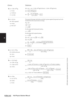
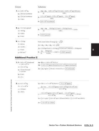
 =
1
2
(8.73 m/s)(20.3 s)
∆x = 88.6 m = 88.6 m to the east
7.58 × 10⁴
kg•m/s
2.03 × 10⁴
kg
−2.44 × 10⁴
kg•m/s + 1.02 × 10⁵
kg•m/s
2.03 × 10⁴
kg
−2.44 × 10⁴
kg•m/s + (2.03 × 10⁴
kg)(5.00 m/s)
2.3 × 10⁴
kg
2.44 × 10⁴
kg•m/s to the west
4. m = 113 g
vi = 2.00 m/s to the right
vf = 0 m/s
∆t = 0.80 s
F =
mvf
∆
−
t
mvi
= =
F = −0.28 N =
∆x =
1
2
(vi + vf)∆t =
1
2
(2.00 m/s + 0 m/s)(0.80 s)
∆x = 0.80 m to the right
0.28 N to the left
−(0.113 kg)(2.00 m/s)
0.80 s
(0.113 kg)(0 m/s) − (0.113 kg)(2.00 m/s)
0.80 s
6. h = 68.6 m
m = 1.00 × 10³
kg
F = −2.24 × 10⁴
N
g = 9.81 m/s2
vf = 0 m/s
From conservation of energy,
vi =
2g
h
∆p = mvf − mvi = mvf − m
2g
h
∆t =
∆
F
p
=
mvf −
F
m
2g
h
=
∆t = =
∆x =
1
2
(vi + vf)∆t =
1
2
(
2g
h
+ vf)∆t
∆x =
1
2
(2
)(
9.
81
m
/s
2
)
(6
8.
6
m
)
+ 0 m/s(1.64 s) = 30.1 m
1.64 s
−(1.00 × 10³
kg)
(2
)(
9.
81
m
/s
2
)
(6
8.
6
m
)
−2.24 × 10⁴
N
(1.00 × 10³
kg)(0 m/s) − (1.00 × 10³
kg)
(2
)(
9.
81
. m
/s
2
)
(6
8.
6
m
)
−2.24 × 10⁴
N
5. m = 4.90 × 10⁶
kg
vi = 0.200 m/s
vf = 0 m/s
∆t = 10.0 s
F =
∆
∆
p
t
=
mvf
∆
−
t
mvi
=
F = –9.80 104
N
F =
∆x =
1
2
(vi + vf)∆t =
1
2
(0.200 m/s + 0 m/s)(10.0 s)
∆x = 1.00 m
9.80 × 10⁴
N opposite the palace’s direction of motion
–(4.90 106
kg)(0.200 m/s)
10.0 s
(4.90 × 10⁶
kg)(0 m/s) − (4.90 × 10⁶
kg)(0.200 m/s)
10.0 s](https://image.slidesharecdn.com/physicssolutions-230306125240-7bc050a7/85/physics-solutions-pdf-375-320.jpg)
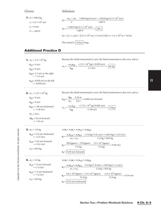
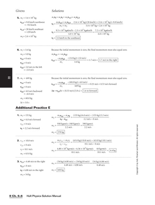


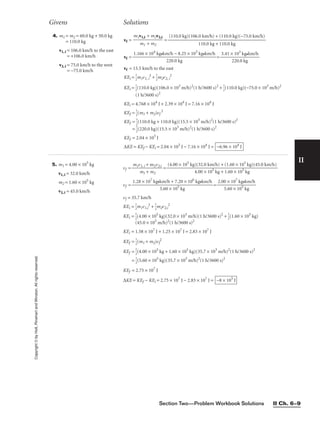

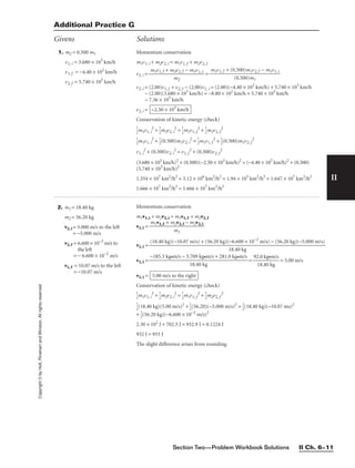
![Givens Solutions
Holt Physics Solution Manual
II Ch. 6–12
II
Copyright
©
by
Holt,
Rinehart
and
Winston.
All
rights
reserved.
3. m1 = m2
v1, i = 5.0 m/s to the right
= +5.0 m/s
v1, f = 2.0 m/s to the left
= −2.0 m/s
v2, f = 5.0 m/s to the right
= +5.0 m/s
Momentum conservation
m1v1, i + m2v2, i = m1v1, f + m2v2, f
v2, i = = v1, f + v2, f − v1, i
v2, i = −2.0 m/s + 5.0 m/s − 5.0 m/s = −2.0 m/s
v2, i =
Conservation of kinetic energy (check)
1
2
miv1, i
2
+
1
2
m2v2, i
2
=
1
2
m1v1, f
2
+
1
2
m2v2, f
2
v1,i
2
+ v2,i
2
= v1,f
2
+ v2,f
2
(5.0 m/s)2
+ (−2.0 m/s)2
= (−2.0 m/s)2
+ (5.0 m/s)2
25 m2
/s2
+ 4.0 m2
/s2
= 4.0 m2
/s2
+ 25 m2
/s2
29 m2
/s2
= 29 m2
/s2
2.0 m/s to the left
m1v1, f + m2v2, f − m1v1, i
m2
4. m1 = 45.0 g
v1, i = 273 km/h to the right
= +273 km/h
v2, i = 0 km/h
v1, f = 91 km/h to the left
= −91 km/h
v2, f = 182 km/h to the right
= +182 km/h
Momentum conservation
m1v1, i + m2v2, i = m1v1, f + m2v2, f
m2 =
m1v
v
1
2
,
,
f
i −
−
v
m
2
1
,
v
f
1, i
=
m2 = =
m2 =
Conservation of kinetic energy (check)
1
2
m1v1,i
2
+
1
2
m2v2,i
2
=
1
2
m1v1, f
2
+
1
2
m2v2, f
1
2
(45.0 g)(273 103
m/h)2
(1 h/3600 s)2
+
1
2
(90.1 g)(0 m/s)2
=
1
2
(45.0 g)(−91 × 103
m/h)2
(1 h/3600 s)2
+
1
2
(90.1 g)(182 × 103
m/h)2
(1 h/3600 s)2
129 J + 0 J = 14 J + 115 J
129 J = 129 J
90.1 g
−16.4 103
g •km/h
−182 km/h
−4.1 103
g •km/h − 12.3 103
g •km/h
−182 km/h
(45.0 g)(−91 km/h) − (45.0 g)(273 km/h)
0 km/h − 182 km/h
5. v1,i = 185 km/h to the right
185 km/h
v2,i = 0 km/h
vi,f = 80.0 km/h to the left
= −80.0 km/h
m1 = 5.70 10–2
kg
Momentum conservation
m1v1, i + m2v2,i = m1v1,f + m2v2,f
m
m
1
2
v1,i −
m
m
1
2
v1,f = v2,f –v2,i
m
m
1
2
[185 km/h − (−80.0 km/h)] = v2,f − 0 km/h
v2,f =
m
m
1
2
(265 km/h) to the right
Conservation of kinetic energy
KEi =
1
2
m1v1,i
2
+
1
2
m2v2,i
2
=
1
2
m1v1,i
2
KEf =
1
2
m1v1,f
2
+
1
2
m2v2,f
2
1
2
m1v1,i
2
=
1
2
m1v1,f
2
+
1
2
m2v2,f
2
m
m
1
2
(v1,i)2
=
m
m
1
2
(v1,f)2
+ v2,f
2
m
m
1
2
(185 km/h)2
=
m
m
1
2
(−80.0 km/h)2
+ v2,f
2](https://image.slidesharecdn.com/physicssolutions-230306125240-7bc050a7/85/physics-solutions-pdf-383-320.jpg)
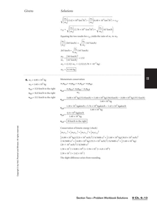

![Section Two—Problem Workbook Solutions II Ch. 7–1
Circular Motion
and Gravitation
Problem Workbook Solutions
II
Copyright
©
by
Holt,
Rinehart
and
Winston.
All
rights
reserved.
Additional Practice A
Givens Solutions
1. vt = 0.17 m/s
ac = 0.29 m/s2
r =
v
a
t
c
2
=
(0
0
.
.
1
2
7
9
m
m
/
/
s
s
)
2
2
= 0.10 m
2. vt = 465 m/s
ac = 3.4 × 10⁻²
m/s2
r =
v
a
t
c
2
=
3.4
(4
×
6
1
5
0
m
−2
/s
m
)2
/s2
= 6.4 × 10⁶
m
3. r =
58.4
2
cm
= 29.2 cm
ac = 8.50 × 10⁻²
m/s2
vt =
ra
c
=
(2
9.
2
×
1
0−
2
m
)(
8.
50
×
1
0−
2
m
/s
2
vt = 0.158 m/s
4. r =
12
2
cm
= 6.0 cm
ac = 0.28 m/s2
vt =
ra
c
=
(6
.0
×
1
0−
2
m
)(
0.
28
m
/s
2
)
= 0.13 m/s
5. vt = 7.85 m/s
r = 20.0 m
ac =
v
r
t
2
=
(7.
2
8
0
5
.0
m
m
/s)2
= 3.08 m/s2
6. ∆t = 1.000 h
∆s = 47.112 km
r = 6.37 × 10³
km
ac =
v
r
t
2
= =
r
∆
∆
s
t
2
2
ac = = 2.69 × 10⁻⁵
m/s2
(47 112 m)2
(6.37 × 10⁶ m)[(1.000 h)(3600 s/h)]2
∆
∆
s
t
2
r
Additional Practice B
1. m1 = 235 kg
m2 = 72 kg
r = 25.0 m
Fc = 1850 N
mtot = m1 + m2 = 235 kg + 72 kg = 307 kg
Fc = mtot ac = mtot
v
r
t
2
vt =
m
r
F
to
c
t
=
(2
5.
0
3
m
0
)
7
(
1
k
8
g
5
0
N
)
= 12.3 m/s
2. m = 30.0 g
r = 2.4 m
FT = 0.393 N
g = 9.81 m/s2
FT = Fg + Fc = mg + m
v
r
t
2
vt =
r(
F
T
m
−
m
g)
=
vt = =
vt = 2.8 m/s
(2.4 m)(0.099 N)
30.0 × 10⁻³
kg
(2.4 m)(0.393 N − 0.294 N)
30.0 × 10⁻³
kg
(2.4 m)[0.393 N − (30.0 × 10⁻³
kg)(9.81 m/s2
)]
30.0 × 10⁻³
kg](https://image.slidesharecdn.com/physicssolutions-230306125240-7bc050a7/85/physics-solutions-pdf-386-320.jpg)
![Holt Physics Solution Manual
II Ch. 7–2
II
Copyright
©
by
Holt,
Rinehart
and
Winston.
All
rights
reserved.
Givens Solutions
2. m1 = 3.08 × 10⁴
kg
r = 1.27 × 10⁷
m
Fg = 2.88 × 10⁻¹⁶
N
G = 6.673 × 10⁻¹¹
N•m2
kg2
m2 = =
m2 = 2.26 × 10⁴
kg
(2.88 × 10⁻¹⁶
N)(1.27 × 10⁷
m)2
6.673 × 10⁻¹¹
N
k
•
g
m
2
2
(3.08 × 10⁴
kg)
Fgr2
Gm1
3. vt = 8.1 m/s
r = 4.23 m
m1 = 25 g
g = 9.81 m/s2
Fg = Fc
m1g =
m2
r
vt
2
m2 =
m
v
1
t
2
gr
m2 = = 1.6 × 10⁻²
kg
(25 × 10−3
kg)(9.81 m/s2
)(4.23 m)
(8.1 m/s)2
4. vt = 75.57 km/h
m = 92.0 kg
Fc = 12.8 N
Fc = m
v
r
t
2
r =
m
F
v
c
t
2
=
r = 3.17 × 10³
m = 3.17 km
(92.0 kg)[(75.57 km/h)(103
m/km)(1 h/3600 s)]2
12.8 N
5. m = 75.0 kg
r = 446 m
vt = 12 m/s
g = 9.81 m/s2
Fc =
m
r
vt
2
= =
FT = Fc + mg = 24 N + (75.0 kg)(9.81 m/s2
)
FT = 24 N + 736 N = 7.60 × 10²
N
24 N
(75.0 kg)(12 m/s)2
446 m
1. r = 6.3 km
Fg = 2.5 × 10⁻²
N
m1 = 3.0 kg
G = 6.673 × 10⁻¹¹
N•m2
kg2
m2 = =
m2 = 5.0 × 10¹⁵
kg
(2.5 × 10⁻²
N)(6.3 × 10³
m)2
6.673 × 10⁻¹¹
N
k
•
g
m
2
2
(3.0 kg)
Fgr2
Gm1
3. m1 = 5.81 × 10⁴
kg
r = 25.0 m
Fg = 5.00 × 10⁻⁷
N
G = 6.673 × 10⁻¹¹
N•m2
kg2
m2 = =
m2 = 80.6 kg
(5.00 × 10⁻⁷
N)(25.0 m)2
6.673 ×10⁻¹¹
N
k
•
g
m
2
2
(5.81 × 10⁴
kg)
Fgr2
Gm1
Additional Practice C](https://image.slidesharecdn.com/physicssolutions-230306125240-7bc050a7/85/physics-solutions-pdf-387-320.jpg)
![Section Two—Problem Workbook Solutions II Ch. 7–3
II
Copyright
©
by
Holt,
Rinehart
and
Winston.
All
rights
reserved.
Givens Solutions
7. m1 = 318mE
m2 = 50.0 kg
VJ = 1323VE
mE = 5.98 × 1024
kg
rE = 6.37 × 10⁶
m
G = 6.673 × 10⁻¹¹
N•m2
kg2
If VJ = 1323 VE, then rJ =
3
13
23
rE.
Fg =
Gm
rJ
1
2
m2
=
Fg = 1.30 × 10³
N
(6.673 × 10⁻¹¹
N•m2
/kg2
)(318)(5.98 × 1024
kg)(50.0 kg)
[(
3
13
23
)(6.37 × 10⁶ m)]2
4. m1 = 621 g
m2 = 65.0 kg
Fg = 1.0 × 10⁻¹²
N
G = 6.673 × 10⁻¹¹
N•m2
kg2
r =
G
m
F
1
g
m
2
r = = 52 m
(6.673 × 10⁻¹¹ N•m2/kg2)(0.621 kg)(65.0 kg)
1.0 × 10⁻¹² N
5. m1 = m2 = 1.0 × 10⁸
kg
Fg = 1.0 × 10⁻³
N
G = 6.673 × 10⁻¹¹
N•m2
kg2
r =
G
m
F
1
g
m
2
r =
r = 2.6 × 10⁴
m = 26 km
(6.673 × 10⁻¹¹ N•m2/kg2)(1.0 × 108
kg)2
1.0 × 10⁻³ N
6. ms = 25 × 109
kg
m1 = m2 =
1
2
ms
r = 1.0 × 10³
km
G = 6.673 × 10⁻¹¹
N•m2
kg2
Fg =
Gm
r
1
2
m2
= = 1.0 × 10⁻²
N
6.673 × 10⁻¹¹
N
k
•
g
m
2
2
1
2
(25 × 109
kg)2
(1.0 × 10⁶ m)2
Additional Practice D
1. T = 88 643 s
m = 6.42 × 10²³
kg
rm = 3.40 × 10⁶
m
r =
3
=
3
r = 2.04 × 10⁷
m
rs = r − rm = 2.04 × 10⁷
m − 3.40 × 10⁶
m = 1.70 × 10⁷
m
6.673 × 10⁻¹¹
N
k
•
g
m
2
2
(6.42 × 10²³
kg)(88 643 s)2
4p2
GmT2
4p2
2. T = 5.51 × 10⁵
s
m = 1.25 × 10²²
kg
r =
3
=
3
r = 1.86 × 10⁷
m
6.673 × 10⁻¹¹
N
k
•
g
m
2
2
(1.25 × 10²²
kg)(5.51 × 10⁵
s)2
4p2
GmT2
4p2](https://image.slidesharecdn.com/physicssolutions-230306125240-7bc050a7/85/physics-solutions-pdf-388-320.jpg)
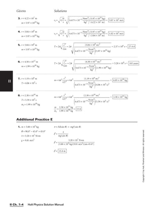
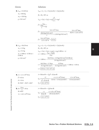
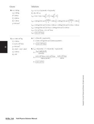
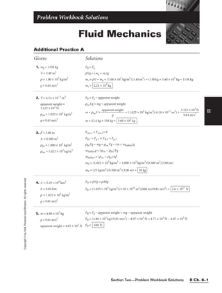
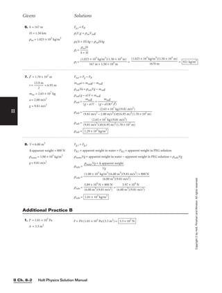


![II
Copyright
©
by
Holt,
Rinehart
and
Winston.
All
rights
reserved.
Section Two—Problem Workbook Solutions II Ch. 9–1
1. TC = 14°C T = TC + 273.15
T = (14 + 273.15) K
T =
TF =
9
5
TC + 32.0
TF =
9
5
(14) + 32.0°F = (25 + 32.0)°F
TF = 57°F
287 K
Additional Practice A
Givens Solutions
2. TF = (4.00 × 10²
)°F TC =
5
9
(TF − 32.0)
TC =
5
9
[(4.00 × 10²
) − 32.0]°C =
5
9
(368)°C
TC =
T = TC + 273.15
T = (204 + 273.15) K
T = 477 K
204°C
3. TC,1 = 117°C
TC,2 = −163°C
∆TC = TC,1 − TC,2 = 117°C − (−163°C)
∆TC = (2.80 × 10²
)°C
∆TF =
5
9
∆TC
∆TF =
5
9
(2.80 × 10²
)°F
∆TF = 504°F
Heat
Problem Workbook Solutions
4. TF = 860.0°F TC =
5
9
(TF − 32.0)
TC =
9
5
(860.0 − 32.0)°C =
9
5
(828.0)°C
TC = 460.0°C](https://image.slidesharecdn.com/physicssolutions-230306125240-7bc050a7/85/physics-solutions-pdf-396-320.jpg)
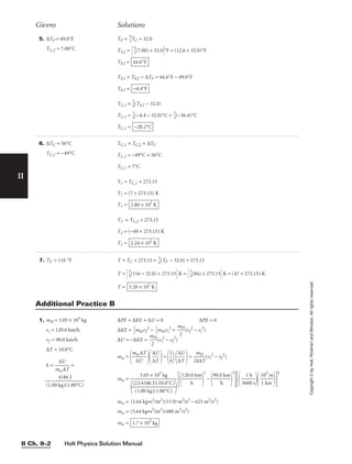
![Section Two—Problem Workbook Solutions II Ch. 9–3
II
Copyright
©
by
Holt,
Rinehart
and
Winston.
All
rights
reserved. 2. h = 228 m
Ti = 0.0°C
g = 9.81 m/s2
fraction of MEf converted
to U = 0.500
k = (∆U/m) = energy
needed to melt ice =
3.33 × 10⁵
J/1.00 kg
∆PE = −mgh
When the ice lands, its kinetic energy is tranferred to the internal energy of the
ground and the ice. Therefore, ∆KE = 0 J.
∆U = (0.500)(MEf ) = −(0.500)(∆PE) = (0.500)(mgh)
∆
m
U
= (0.500)(gh)
f =
∆
km
U
=
(0.500
k
)(gh)
f =
f = 3.36 × 10⁻³
(0.500)(9.81 m/s2
)(228 m)
(3.33 × 10⁵ J/1.00 kg)
Givens Solutions
3. vi = 2.333 × 10³
km/h
h = 4.000 × 10³
m
g = 9.81 m/s2
fraction of ME converted
to U = 0.0100
k =
m
∆
∆
U
T
=
(1.00 k
(3
g
5
)(
5
1
J
.
)
00°C)
4. h = 8848 m
g = 9.81 m/s2
fraction of MEf converted
to U = 0.200
Ti = −18.0°C
∆U
∆T
/m
=
4
1
4
.
8
00
J
°
/k
C
g
∆PE = −mgh
MEf = −∆PE
When the hook lands, its kinetic energy is transferred to the internal energy of the
hook and the ground. Therefore, ∆KE = 0 J.
∆U = (0.200)(MEf) = (−0.200)(∆PE) = (0.200)(mgh)
∆U/m = (0.200)(gh)
∆T =
∆U
∆T
/m
∆
m
U
=
4
1
4
.
8
00
J
°
/k
C
g
[(0.200)(gh)]
∆T =
4
1
4
.
8
00
J
°
/k
C
g
(0.200)(9.81 m/s2
)(8848 m) = 38.7°C
Tf = Ti + ∆T = −18.0°C + 38.7°C
Tf = 20.7°C
(0.0100)(∆PE + ∆KE) + ∆U = 0
∆PE = PEf − PEi = 0 − mgh = −mgh
∆KE = KEf − KEi = 0 −
1
2
mvi
2
= −
1
2
mvi
2
∆U = −(0.0100)(∆PE + ∆KE) = −(0.0100)(m)−gh −
1
2
v2
= (0.0100)(m)gh +
1
2
v2
∆T = =
∆T =
∆T =
∆T = 7.02°C
(0.0100)[(3.92 × 10⁴
m2
/s2
) + (2.100 × 10⁵
m2
/s2
)]
355 m2/s2•°C
(0.0100)
(9.81 m/s2)(4.000 × 103
m) +
1
2
2.33
3
3
6
×
00
10
s/
6
h
m/h
2
355 m2/s2•°C
(0.0100)gh +
1
2
v2
(1.00 k
3
g
5
)
5
(1
J
.00°C)
∆
m
U
k](https://image.slidesharecdn.com/physicssolutions-230306125240-7bc050a7/85/physics-solutions-pdf-398-320.jpg)
![Holt Physics Solution Manual
II Ch. 9–4
II
Copyright
©
by
Holt,
Rinehart
and
Winston.
All
rights
reserved.
7. ∆T = 0.230°C
g = 9.81 m/s2
fraction of MEf converted
to U = 0.100
∆
∆
U
T
/m
=
41
1
8
.0
6
0
J
°
/
C
kg
∆
m
U
= ∆T
∆
∆
U
T
/m
=
(0.100
m
)(MEf )
=
(0.100
m
)(∆PE)
= (0.100)(gh)
Because the kinetic energy at the bottom of the falls is converted to the internal en-
ergy of the water and the ground, ∆KE = 0 J.
h =
h =
41
1
8
.0
6
0
J
°
/
C
kg
h = 981 m
0.230°C
(0.100)(9.81 m/s2)
∆T
∆
∆
U
T
/m
(0.100)(g)
5. hi = 629 m
g = 9.81 m/s2
vf = 42 m/s
fraction of ME converted
to U = 0.050
m = 3.00 g
Because hf = 0 m, PEf = 0 J. Further, vi = 0 m/s, so KEi = 0 J.
∆U = −(0.050)(∆ME) = −(0.050)(∆PE + ∆KE)
∆PE = PEf − PEi = 0 J − PEi = −mgh
∆KE = KEf − KEi = KEf − 0 J =
1
2
mvf
2
∆U = (0.050)(−∆PE − ∆KE) = (0.050)(mgh −
1
2
mvf
2
) = (0.050)(m)(gh −
1
2
vf
2
)
∆U = (0.050)(3.00 × 10⁻³
kg)[(9.81 m/s2
)(629 m) − (0.5)(42 m/s)2
]
∆U = (0.050)(3.00 × 10⁻³
kg)(6170 m2
/s2
− 880 m2
/s2
)
∆U = (0.050)(3.00 × 10⁻³
kg)(5290 m2
/s2
)
∆U = 0.79 J
Givens Solutions
6. h = 2.49 m
g = 9.81 m/s2
m = 312 kg
v = 0.50 m/s
fraction of ME converted
to U = 0.500
(0.500)(∆PE + ∆KE) + ∆U = 0
∆PE = PEf − PEi = 0 − mgh = −mgh
∆KE = KEf − KEi = 0 −
2
1
mv2
=
−m
2
v2
∆U = −(0.500)(∆PE + ∆KE) = −(0.500)
−mgh −
m
2
v2
= (0.500)
mgh +
m
2
v2
∆U = (0.500)[(312 kg)(9.81 m/s2)(2.49 m) + (0.5)(312 kg)(0.50 m/s)2
]
∆U = (0.500)[(7.62 × 10³
J) + 39 J]
∆U = 3.83 × 10³
J](https://image.slidesharecdn.com/physicssolutions-230306125240-7bc050a7/85/physics-solutions-pdf-399-320.jpg)
![Section Two—Problem Workbook Solutions II Ch. 9–5
II
Copyright
©
by
Holt,
Rinehart
and
Winston.
All
rights
reserved.
1. Q = (2.8 × 10⁹
W)(1.2 s)
cp,c = 387 J/kg•°C
Tc = 26.0°C
Tf = 21.0°C
Q = −mccp,c(Tf − Tc) = mccp,c(Tc − Tf )
mc =
cp,c(T
Q
c − Tf )
mc =
mc = = 1.7 × 10⁶
kg
(2.8 × 10⁹
W)(1.2 s)
(387 J/kg•°C)(5.0°C)
(2.8 × 10⁹
W)(1.2 s)
(387 J/kg•°C)(26.0°C − 21.0°C)
2. mw = 143 × 103
kg
Tw = 20.0°C
Tx = temperature of
burning wood = 280.0°C
Tf = 100.0°C
cp,x = specific heat
capacity of wood =
1.700 × 10³
J/kg•°C
cp,w = 4186 J/kg•°C
− cp,xmx (Tf − Tx) = cp,wmw(Tf − Tw)
mx =
mx =
mx =
mx = 1.56 × 10⁵
kg
(4186 J/kg•°C)(143 × 103
kg)(80.0°C)
(1.700 × 10³ J/kg•°C)(180.0°C)
(4186 J/kg•°C)(143 × 103
kg)(100.0°C − 20.0°C)
(1.700 × 10³ J/kg•°C)(280.0°C − 100.0°C)
cp,wmw(Tf − Tw)
cp,x(Tx − Tf )
Additional Practice C
Givens Solutions
3. ∆U = Q = (0.0100)
(1.450 GW)(1.00 year)
cp,x = specific heat capacity
of iron = 448 J/kg•°C
mx = mass of steel =
25.1 × 10⁹
kg
Q = cp,x mx ∆T
∆T =
cp,x
Q
mx
∆T =
365
1
.2
y
5
ea
d
r
ays
1
2
d
4
a
h
y
36
1
0
h
0 s
∆T = 40.7°C
(0.0100)(1.450 × 10⁹
W)(1.00 year)
(448 J/kg•°C)(25.1 × 109
kg)
4. ml = 2.25 × 10³
kg
Tl,i = 28.0°C
cp,l = cp,w = 4186 J/kg•°C
mi = 9.00 × 10²
kg
Ti,i = −18.0°C
cp,i = 2090 J/kg•°C
Ti,f = 0.0°C
−mlcp,l (Tl,f − Tl,i) = micp,i(Ti,f − Ti,i)
Tl,f = Tl,i −
m
m
l
i
c
c
p
p
,
,
l
i
(Ti,f − Ti,i)
Tl,f = (28.0°C) −
2
9
.
.
2
0
5
0
×
×
1
1
0
0
3
2
k
k
g
g
[(0.0°C) − (−18.0°C)]
Tl,f = 28.0°C − 3.59°C = 24.4°C
2090 J/kg•°C
4186 J/kg•°C
5. mw = 1.33 × 10¹⁹
kg
Tw = 4.000°C
cp,w = 4186 J/kg•°C
P = 1.33 × 10¹⁰
W
∆t = 1.000 × 10³
years
P∆t = Q = mwcp,w(Tf − Tw)
Tf =
m
P
w
∆
cp
t
,w
+ Tw
Tf = + 4.000°C
Tf = (7.54 × 10⁻³
)°C + 4.000°C
Tf = 4.008°C
(1.33 × 10¹⁰
W)(1.000 × 10³
years)
36
1
5.
y
2
e
5
a
d
r
ay
1
2
d
4
a
h
y
36
1
0
h
0 s
(1.33 × 10¹⁹ kg)(4186 J/kg•°C)](https://image.slidesharecdn.com/physicssolutions-230306125240-7bc050a7/85/physics-solutions-pdf-400-320.jpg)
![Holt Physics Solution Manual
II Ch. 9–6
II
Copyright
©
by
Holt,
Rinehart
and
Winston.
All
rights
reserved.
7. Tm = −62.0°C
Tw = 38.0°C
mm = 180 g
mw = 0.500 kg
Tf = 36.9°C
cp,w = 4186 J/kg•°C
mmcp,m(Tf − Tm) = −mwcp,w(Tf − Tw)
cp,m =
m
m
m
w
(cp,w)
T
T
f
w
−
−
T
T
m
f
cp,m =
0
0
.5
.1
0
8
0
k
k
g
g
(4186 J/kg•°C)
cp,m =
The metal could be gold (cp = 129 J/kg•°C) or lead (cp = 128 J/kg•°C).
1.3 × 10²
J/kg•°C
(38.0°C) − (36.9°C)
(36.9°C) − (−62.0°C)
Givens Solutions
6. Ti = 18.0°C
Tf = 32.0°C
Q = 20.8 kJ
mx = 0.355 kg
Q = mxcp,x∆T
cp,x =
mx
Q
∆T
=
mx(T
Q
f − Ti)
cp,x =
cp,x = 4190 J/kg•°C
20.8 × 10³
J
(0.355 kg)(32.0°C − 18.0°C)
1. mw,S = 1.20 × 10¹⁶
kg
mw,E = 4.8 × 10¹⁴
kg
TE = 0.0°C
TS = 100.0°C
cp,w = 4186 J/kg•°C
Lf of ice = 3.33 × 10⁵
J/kg
QS = energy transferred by heat from Lake Superior = cp,wmw,S(TS − Tf)
QE = energy transferred by heat to Lake Erie = mw,ELf + mw,Ecp,w(Tf − TE)
From the conservation of energy,
QS = QE
cp,wmw,S(TS − Tf ) = mw,ELf + mw,Ecp,w(Tf − TE)
(mw,Ecp,w + cp,wmw,S)Tf = cp,wmw,STS + mw,Ecp,wTE − mw,ELf
Tf = , where TE = 0.0°C
Tf =
Tf =
Tf =
Tf = 92.9°C
(5.02 × 10²¹
J) − (1.6 × 10²⁰
J)
(4186 J/kg•°C)(1.25 × 1016 kg)
(4186 J/kg•°C)(1.20 × 1016
kg)(100.0°C) − (4.8 × 10¹⁴
kg)(3.33 × 10⁵
J/kg)
(4186 J/kg•°C)[(4.8 × 1014
kg) + (1.20 × 10¹⁶
kg)]
cp,wmw,STS − mw,ELf
cp,w (mw,E + mw,S)
cp,w(mw,STS + mw,ETE) − mw,ELf
cp,w (mw,E + mw,S)
Additional Practice D
2. Tf = −235°C
Tfreezing = 0.0°
mw = 0.500 kg
cp,w = 4186 J/kg•°C
cp,ice = cp,i = 2090 J/kg•°C
Lf of ice = 3.33 × 10⁵
J/kg
Qtot = 471 kJ
Qtot = cp,wmw(Ti − 0.0°) + Lf mw + mwcp,i(0.0°− Tf) = cp,wmwTi + Lf mw − cp,imwTf
Ti =
Ti =
Ti =
Ti = 28°C
(4.71 × 10⁵
J) − (1.66 × 10⁵
J) − (2.46 × 10⁵
J)
2093 J/°C
(4.71 × 10⁵
J) − (3.33 × 10⁵
J/kg)(0.500 kg) + (−235°C)(2090 J/kg•°C)(0.500 kg)
(4186 J/kg•°C)(0.500 kg)
Qtot − Lf mw + cp,imwTf
cp,wmw](https://image.slidesharecdn.com/physicssolutions-230306125240-7bc050a7/85/physics-solutions-pdf-401-320.jpg)
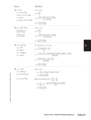
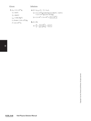
![II
Copyright
©
by
Holt,
Rinehart
and
Winston.
All
rights
reserved.
Section Two—Problem Workbook Solutions II Ch. 10–1
1. P = 5.1 kPa
W = 3.6 × 10³
J
Vi = 0.0 m3
W = P∆V
∆V =
W
P
=
5
3
.1
.6
×
×
1
1
0
0
3
3
P
J
a
= 7.1 × 10⁻¹
m3
V = Vi + ∆V = 0.0 m3
+ 7.1 × 10⁻¹
m3
= 7.1 × 10⁻¹
m3
Additional Practice A
Givens Solutions
2. m = 207 kg
g = 9.81 m/s2
h = 3.65 m
P = 1.8 × 10⁶
Pa
W = mgh = −P∆V
∆V =
m
−
g
P
h
∆V = = −4.1 × 10⁻³
m3
(207 kg)(9.81 m/s2
)(3.65 m)
−(1.8 × 10⁶ Pa)
3. rf = 1.22 m
ri = 0.0 m
W = 642 kJ
W = P∆V
P =
∆
W
V
∆V =
3
4
p(rf
3
− ri
3
)
P = = = 8.44 × 10⁴
Pa
642 × 103
J
3
4
p (1.22 m)3 − (0.0 m)3
W
3
4
p(rf
3 − ri
3)
4. rf = 7.0 × 10⁵
km
rf = 7.0 × 10⁸
m
ri = 0.0 m
W = 3.6 × 1034
J
W = P∆V
V =
3
4
pr3
∆V = Vf − Vi =
3
4
p(rf
3
− ri
3
)
W = (P)(
3
4
p)(rf
3
− ri
3
)
P = W
(
3
4
p)(rf
3 − ri
3)
5. P = 87 kPa
∆V = −25.0 × 10⁻³
m3
W = P∆V
W = (87 × 103
Pa)(−25.0 × 10⁻³
m3
) = −2.2 × 10³
J
Thermodynamics
Problem Workbook Solutions
P = = 2.5 × 10⁷
Pa
(3.6 × 1034
J)
(
3
4
p )[(7.0 × 10⁸
m)3
− (0.0 m)3
]](https://image.slidesharecdn.com/physicssolutions-230306125240-7bc050a7/85/physics-solutions-pdf-404-320.jpg)
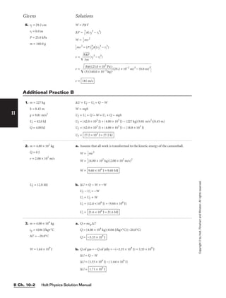
![Section Two—Problem Workbook Solutions II Ch. 10–3
II
Copyright
©
by
Holt,
Rinehart
and
Winston.
All
rights
reserved.
6. P =
∆
Q
t
= 5.9 × 10⁹
J/s
∆t = 1.0 s
∆U = 2.6 × 10⁹
J
∆U = Q − W = P∆t − W
W = P∆t − ∆U
W = (5.9 × 10⁹
J/s)(1.0 s) − (2.6 × 10⁹
J)
W = 3.3 × 10⁹
J
Givens Solutions
5. m = 5.00 × 10³
kg
v = 40.0 km/h
Ui = 2.50 × 10⁵
J
Uf = 2Ui
W =
1
2
mv2
∆U = Uf − Ui = Q − W
Uf = 2Ui
∆U = 2Ui − Ui = Ui
Q = ∆U + W = Ui +
1
2
mv2
Q = (2.50 × 10⁵
J) +
1
2
(5.00 × 10³
kg)
40.0
h
km
36
1
0
h
0 s
1
1
0
k
3
m
m
2
Q = (2.50 × 10⁵
J) + (3.09 × 10⁵
J)
Q = 5.59 × 10⁵
J
4. m = 1.64 × 10¹⁵
kg
h = 75.0 m
g = 9.81 m/s2
Ti = 6.0°C
Tf = 100.0°C
cp,w = 4186 J/kg•°C
Lv of water = 2.26 × 10⁶
J/kg
∆U = (−0.900)(Ui)
W = mgh = (1.64 × 10¹⁵
kg)(9.81 m/s2
)(75.0 m)
W = 1.21 × 10¹⁸
J
Q = −mcp,w(Tf − Ti) − mLv = −m[cp,w(Tf − Ti) + Lv]
Tf − Ti = 100.0°C − 6.0°C = 94.0°C
Q = −(1.64 × 10¹⁵
kg)[(4186 J/kg•°C)(94.0°C) + (2.26 × 10⁶
J/kg)]
Q = −4.35 × 10²¹
J
∆U = Uf − Ui = (−0.900)(Ui) = Q − W
Uf = (1 − 0.900)Ui = (0.100)(Ui)
−∆U = Ui − Uf =
0.
U
10
f
0
− Uf = (0.900)
0.
U
10
f
0
= W − Q
Uf =
0
0
.
.
1
9
0
0
0
0
(W − Q)
Uf =
0
0
.
.
1
9
0
0
0
0
[(1.21 × 10¹⁸
J) − (−4.35 × 10²¹
J)]
Uf =
(Note: Nearly all of the energy is used to increase the temperature of the water
and to vaporize the water.)
4.83 × 10²⁰
J](https://image.slidesharecdn.com/physicssolutions-230306125240-7bc050a7/85/physics-solutions-pdf-406-320.jpg)
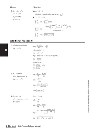
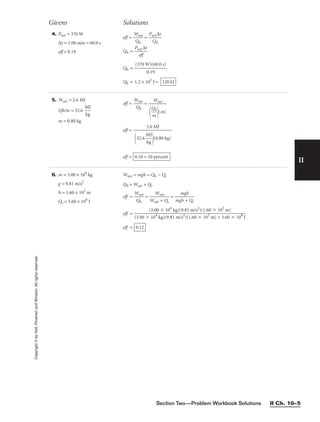

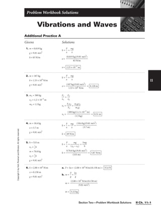
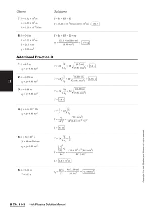
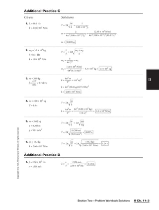
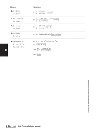


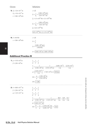


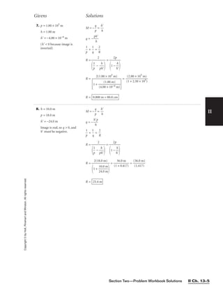


![Section Two—Problem Workbook Solutions II Ch. 14–5
II
Copyright
©
by
Holt,
Rinehart
and
Winston.
All
rights
reserved. 10. p = 117 × 10−3
m
M = 2.4
M = −
p
q
q = −pM = −(117 × 10−3
m)(2.4)
q = − 0.28 m
p
1
+
q
1
=
1
f
1
f
=
(117 ×
1
10−3 m)
−
(0.2
1
8 m)
=
8
1
.5
m
5
−
1
3.
m
6
=
1
5.
m
0
f = 0.20 m = 2.0 × 10²
mm
Givens Solutions
11. Image is real, and therefore
inverted.
h
h
= M = −64
q = 12 m
p = −
M
q
p
1
+
q
1
=
1
f
−
M
q
+
q
1
=
1
f
f =
(1 −
q
M)
f =
[1
(
−
12
(−
m
6
)
4)]
f = Image is inverted
0.18 m = 18 cm
12. h = −0.55 m
h = 2.72 m
p = 5.0 m
−
p
q
=
h
h
q = −
p
h
h
p
1
+
q
1
=
1
f
1
f
=
p
1
−
p
h
h
1
f
=
p
1
1 −
h
h
f =
f = =
5.
5
0
.9
m
f = 0.85 m
5.0 m
1 −
(
(
−
2
0
.7
.5
2
5
m
m
)
)
p
1 −
h
h
](https://image.slidesharecdn.com/physicssolutions-230306125240-7bc050a7/85/physics-solutions-pdf-430-320.jpg)

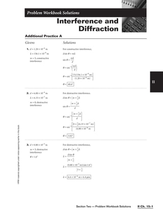
![Holt Physics Solution Manual
II Ch. 15–2
4. d = 15.0 × 10⁻⁶
m
m = 2; constructive
interference
q = 19.5°
For constructive interference,
dsin q = ml
l =
ds
m
in q
l =
l = 2.50 × 10⁻⁶
m = 2.50 mm
(15.0 × 10⁻⁶
m)[sin(19.5°)]
2
6. f = 60.0 × 10³
Hz
c = 3.00 × 10⁸
m/s
m = 4; constructive
interference
q = 52.0°
For constructive interference,
dsin q = ml =
m
f
c
d =
f s
m
in
c
q
d =
d = 2.54 × 10⁴
m = 25.4 km
(4)(3.00 × 10⁸
m/s)
(60.0 × 10³ Hz)(sin 52.0°)
7. f = 137 × 106
Hz
c = 3.00 × 10⁸
m/s
m = 2; constructive
interference
q = 60.0°
For constructive interference,
dsin q = ml =
m
f
c
d =
f s
m
in
c
q
d =
d = 5.06 m
(2)(3.00 × 10⁸
m/s)
(137 × 106 Hz)(sin 60.0°)
mmax =
d(sin
l
90.0°)
=
l
d
=
d
c
f
mmax = = 2.31
The second-order maximum (m = 2) is the highest observable with this apparatus.
(5.06 m)(137 × 106
Hz)
(3.00 × 10⁸ m/s)
Givens Solutions
5. l = 443 × 10−9
m
m = 4; destructive
interference
q = 2.27°
For destructive interference,
dsin q = m +
1
2
l
d =
d =
d = 5.03 × 10⁻⁵
m
4 +
1
2
(443 × 10−9
m)
(sin 2.27°)
m +
1
2
l
sin q
II
Copyright
©
by
Holt,
Rinehart
and
Winston.
All
rights
reserved.](https://image.slidesharecdn.com/physicssolutions-230306125240-7bc050a7/85/physics-solutions-pdf-435-320.jpg)
![Section Two — Problem Workbook Solutions II Ch. 15–3
II
Copyright
©
by
Holt,
Rinehart
and
Winston.
All
rights
reserved.
4. l = 40.0 × 10⁻⁹
m
d = 150.0 × 10⁻⁹
m
m = 2
d(sin q) = ml
q = sin−1
m
d
l
q = sin−1
q = 32.2°
2(40.0 × 10⁻⁹
m)
(150.0 × 10⁻⁹ m)
Additional Practice B
Givens Solutions
1. d =
1.00 × 10
1
2
lines/m
m = 1
q = 30.0°
c = 3.00 × 10⁸
m/s
d(sin q) = ml
l =
d(si
m
n q)
l =
l =
f =
l
c
=
(
(
3
5
.
.
0
0
0
0
×
×
1
1
0
0
8
−3
m
m
/s
)
)
f = 6.00 × 10¹⁰
Hz = 60.0 Ghz
5.00 × 10⁻³
m = 5.00 mm
[sin(30.0°)]
(1.00 × 10²
lines/m)(1)
3. l = 714 × 10−9
m
m = 3
q = 12.0°
d(sin q) = ml
d =
(s
m
in
l
q)
d =
(3)
[
(
s
7
i
1
n
4
(
×
12
1
.0
0
°
−
)
9
]
m)
d =
or
9.71 × 10⁴
lines/m
1.03 × 10⁻⁵
m between lines
2. d = 2.0 × 10⁻⁸
m
m = 3
q = 12°
d(sin q) = ml
l =
d(si
m
n q)
l =
l = 1.4 × 10⁻⁹
m = 1.4 nm
(2.0 × 10⁻⁸
m)[sin(12°)]
3](https://image.slidesharecdn.com/physicssolutions-230306125240-7bc050a7/85/physics-solutions-pdf-436-320.jpg)
![Holt Physics Solution Manual
II Ch. 15–4
II
Copyright
©
by
Holt,
Rinehart
and
Winston.
All
rights
reserved.
6. l = 2.2 × 10⁻⁶
m
d =
6.4 × 10
1
4 lines/m
q = 34.0°
d(sin q) = ml
m =
d(si
l
n q)
m = = 4.0
m = 4.0
[sin (34.0°)]
(6.4 × 10⁴ lines/m)(2.2 × 10−6 m)
5. f = 1.612 × 10⁹
Hz
c = 3.00 × 10⁸
m/s
d = 45.0 × 10⁻²
m
m = 1
d(sin q) = ml =
m
f
c
q = sin−1
m
df
c
q = sin−1
q = 24.4°
(1)(3.00 × 10⁸
m/s)
(45.0 × 10⁻² m)(1.612 × 10⁹ Hz)
Givens Solutions
7. d =
25 × 104
1
lines/m
l = 7.5 × 10⁻⁷
m
q = 48.6°
d(sin q) = ml
m =
d(si
l
n q)
m = = 4.0
m = 4.0
[sin(48.6°)]
(25 × 104 lines/m)(7.5 × 10−7 m)](https://image.slidesharecdn.com/physicssolutions-230306125240-7bc050a7/85/physics-solutions-pdf-437-320.jpg)
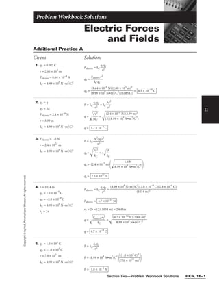

![Section Two—Problem Workbook Solutions II Ch. 16–3
II
Copyright
©
by
Holt,
Rinehart
and
Winston.
All
rights
reserved.
2. q1 = 2.0 × 10⁻⁹
C
q2 = 3.0 × 10⁻⁹
C
q3 = 4.0 × 10⁻⁹
C
q4 = 5.5 × 10⁻⁹
C
r1,2 = 5.00 × 10²
m
r1,3 = 1.00 × 10³
m
r1,4 = 1.747 × 10³
m
kC = 8.99 × 10⁹
N•m2
/C2
3. w = 7.00 × 10⁻²
m
L = 2.48 × 10⁻¹
m
q = 1.0 × 10⁻⁹
C
kC = 8.99 × 10⁹
N•m2
/C2
F = kC
q
r
1q
2
2
Fx = F1 + F2(cos q) = F1 + F2
Fx = kCq2
L
1
2
+
(w2 +
L
L2)3/2
Fx = kCq2
(2.48 × 1
1
0−1 m)2
+
Fx = (8.99 × 10⁹
N•m2
/C2
)(1.0 × 10⁻⁹
C)2
(30.8/m2
) = 2.8 × 10⁻⁷
N
Fy = F3 + F2(sin q) = F3 + F2
Fy = kCq2
w
1
2
+
(w2 +
w
L2)3/2
Fy = kCq2
(7.00 × 1
1
0−2 m)2
+
Fy = (8.99 × 10⁹
N•m2
/C2
)(1.0 × 10⁻⁹
C)2
(2.00 × 10²
/m2
) = 1.8 × 10⁻⁶
N
Fnet =
F
x
2
+
F
y
2
=
(2
.8
×
1
0−
7
N
)2
+
(
1.
8
×
1
0−
6
N
)2
Fnet = 1.8 × 10⁻⁶
N
q = tan−1
F
F
x
y
= tan−1
1
2
.
.
8
8
×
×
1
1
0
0
−
−
6
7
N
N
= 81°
Fnet = 1.8 × 10⁻⁶
N, 81° above the positive x-axis
7.00 × 10⁻² m
[(7.00 × 10⁻² m)2 + (2.48 × 10⁻¹ m)2]3/2
w
w
2
+
L
2
2.48 × 10⁻¹ m
[(7.00 × 10⁻² m)2 + (2.48 × 10⁻¹ m)2]3/2
L
w
2
+
L
2
1. q1 = 2.80 × 10⁻³
C
q2 = −6.40 × 10⁻³
C
q3 = 4.80 × 10⁻²
C
r1,3 = 9740 m
r1,2 = 892 m
kC = 8.99 × 10⁹
N•m2
/C2
F = kC
q
r
1q
2
2
F1,2 = = 2.02 × 10⁻¹
N
F1,3 = = 1.27 × 10⁻²
N
F1,tot = F1,2 + F1,3 = −(2.02 × 10⁻¹
N) + (1.27 × 10⁻²
N) = −0.189 N
F1,tot = 0.189 N downward
(8.99 × 10⁹
N•m2
/C2
)(2.80 × 10⁻³
C)(4.80 × 10⁻²
C)
(9740 m)2
(8.99 × 10⁹
N•m2
/C2
)(2.80 × 10⁻³
C)(6.40 × 10⁻³
C)
(892 m)2
Additional Practice B
Givens Solutions
F = kC
q
r
1q
2
2
F1,2 = = 2.2 × 10⁻¹³
N
F1,3 = = 7.2 × 10⁻¹⁴
N
F1,4 = = 3.2 × 10⁻¹⁴
N
F1,tot = F1,2 + F1,3 + F1,4 = (2.2 × 10⁻¹³
N) + (7.2 × 10⁻¹⁴
N) + (3.2 × 10⁻¹⁴
N)
F1,tot = 3.2 × 10⁻¹³
N down the rope
(8.99 × 10⁹
N•m2
/C2
)(2.0 × 10⁻⁹
C)(5.5 × 10⁻⁹
C)
(1.747 × 10³ m)2
(8.99 × 10⁹
N•m2
/C2
)(2.0 × 10⁻⁹
C)(4.0 × 10⁻⁹
C)
(1.00 × 10³ m)2
(8.99 × 10⁹
N•m2
/C2
)(2.0 × 10⁻⁹
C)(3.0 × 10⁻⁹
C)
(5.00 × 10² m)2](https://image.slidesharecdn.com/physicssolutions-230306125240-7bc050a7/85/physics-solutions-pdf-440-320.jpg)
![Holt Physics Solution Manual
II Ch. 16–4
II
Copyright
©
by
Holt,
Rinehart
and
Winston.
All
rights
reserved.
4. L = 10.7 m
w = 8.7 m
q1 = −1.2 × 10⁻⁸
C
q2 = 5.6 × 10⁻⁹
C
q3 = 2.8 × 10⁻⁹
C
q4 = 8.4 × 10⁻⁹
C
kC = 8.99 × 10⁹
N•m2
/C2
5. d = 1.2 × 10³
m
q1 = 1.6 × 10⁻²
C
q2 = 2.4 × 10⁻³
C
q3 = −3.2 × 10⁻³
C
q4 = −4.0 × 10⁻³
C
kC = 8.99 × 10⁹
N•m2
/C2
∆x = ∆y = = = 8.5 × 10²
m
F =
kC
r
q
2
1q2
Fx = −F2 + F3(cos 45°) = kCq1−
∆
q
x
2
2
+
q3(co
d
s
2
45°)
Fx = (8.99 × 10⁹
N•m2
/C2
)(1.6 × 10⁻²
C)
−
(8
2
.
.
5
4
×
×
1
1
0
0
2
−3
m
C
)2
+
Fx = −0.24 N
Fy = −F4 − F3(sin 45°) = kCq1
∆
q
y
4
2
+
q3(si
d
n
2
45°)
Fy = −(8.99 × 10⁹
N•m2
/C2
)(1.60 × 10⁻²
C)
(8
4
.
.
5
0
×
×
1
1
0
0
2
−3
m
C
)2
+
Fy = −1.0 N
Fnet =
F
x
2
+
F
y
2
=
(0
.2
4
N
)2
+
(
1.
0
N
)2
= 1.0 N
q = tan−1
F
F
x
y
= tan−1
(
(
0
1
.
.
2
0
4
N
N
)
)
= 77°
Fnet = 1.0 N, 77° below the negative x-axis
(3.2 × 10⁻³
C)(sin 45°)
(1.2 × 10³ m)2
(3.2 × 10⁻³
C)(cos 45°)
(1.2 × 10³ m)2
1.2 × 10³
m
2
d
2
Givens Solutions
F = kC
q
r
1q
2
2
Fx = F4 + F3(cos q)
Fy = F2 + F3(sin q)
Fx = kCq1
L
q4
2
+
(L2 +
q3
w
L
2)3/2
Fx = (8.99 × 10⁹
N•m2
/C2
)(1.2 × 10⁻⁸
C)
(8.
(
4
10
×
.7
10
m
−9
)2
C)
+
Fx = 9.1 × 10⁻⁹
N
Fy = kCq1
w
q2
2
+
(L2 +
q3
w
w
2)3/2
Fy = (8.99 × 10⁹
N•m2
/C2
)(1.2 × 10⁻⁸
C)
(5.6
(8
×
.7
1
m
0−
)
9
2
C)
+
Fy = 9.0 × 10⁻⁹
N
Fnet =
F
x
2
+
F
y
2
=
(9
.1
×
1
0−
9
N
)2
+
(
9.
0
×
1
0−
9
N
)2
= 1.28 × 10⁻⁸
N
q = tan−1
F
F
x
y
= tan−1
9
9
.
.
1
0
×
×
1
1
0
0
−
−
9
9
N
N
)
= 45°
Fnet = 1.28 × 10⁻⁸
N, 45° above the positive x-axis
(2.8 × 10⁻⁹
C)(8.7 m)
[(10.7 m)2 + (8.7 m)2]3/2
(2.8 × 10⁻⁹
C)(10.7 m)
[(10.7 m)2 + (8.7 m)2]3/2](https://image.slidesharecdn.com/physicssolutions-230306125240-7bc050a7/85/physics-solutions-pdf-441-320.jpg)
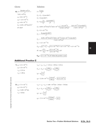
![Holt Physics Solution Manual
II Ch. 16–6
II
Copyright
©
by
Holt,
Rinehart
and
Winston.
All
rights
reserved.
3. mE = 6.0 × 1024
kg
mm = 7.3 × 10²²
kg
G = 6.673 × 10⁻¹¹
N•m2
/kg2
kC = 8.99 × 10⁹
N•m2
/C2
Fg = Felectric
Gm
r
E
2
mm
=
kC
r2
q2
q =
G
m
k
E
C
m
m
=
q = 5.7 × 10¹³
C
(6.673 × 10⁻¹¹
N•m2
/kg2
)(6.0 × 1024
kg)(7.3 × 10²²
kg)
8.99 × 10⁹ N•m2/C2
4. m = 17.23 kg
r = 0.800 m
Fnet = 167.6 N
g = 9.81 m/s2
kC = 8.99 × 10⁹
N•m2
/C2
Fnet = Fg − Felectric
Fnet = mg −
kC
r2
q2
q =
q =
q = 1.0 × 10⁻⁵
C
(0.800 m)2[(17.23 kg)(9.81 m/s2) − (167.6 N)]
8.99 × 10⁹ N•m2/C2
r2
(mg − Fnet)
kC
5. m1 = 9.00 kg
m2 = 8.00 kg
r = 1.00 m
kC = 8.99 × 10⁹
N•m2
/C2
g = 9.81 m/s2
Fg,1 = Fg,2 + Felectric
g(m1 − m2) =
kC
r2
q2
q =
gr
2
(
m
k
1
C
−
m
2)
=
q = 3.30 × 10⁻⁵
C
(9.81 m/s2)(1.00 m)2(9.00 kg − 8.00 kg)
8.99 × 10⁹
N•m2
/C2
6. m = 9.2 × 10⁴
kg
l1 = 1.00 m
g = 9.81 m/s2
l2 = 8.00 m
r = 2.5 m
kC = 8.99 × 10⁹
N•m2
/C2
t1 = t2
mgl1 =
kC
r
q
2
2
l2
q =
r2
k
m
C
l
g
2
l1
q = = 8.9 × 10⁻³
C
(2.5 m)2
(9.2 × 10⁴
kg)(9.81 m/s2
)(1.00 m)
(8.99 × 10⁹ N•m2/C2)(8.00 m)
Givens Solutions
7. q1 = 2.0 C
q2 = 6.0 C
q3 = 4.0 C
L = 2.5 × 10⁹
m
Fnet = 0 = F1 + F2 kC
q
x
1q
2
3
=
(
k
L
C
−
q2
x
q
)
3
2
x
q
2
1
=
(L
q
−
2
x)2
(L − x)
q1
= x
q2
L
x
−
x
x
=
q
q
2
1
L
x
=
q
q
2
1
+ 1
x = = = 9.3 × 10⁸
m
2.5 × 10⁹
m
6
2
.
.
0
0
C
C
+ 1
L
q
q
2
1
+ 1](https://image.slidesharecdn.com/physicssolutions-230306125240-7bc050a7/85/physics-solutions-pdf-443-320.jpg)
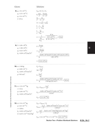
![Holt Physics Solution Manual
II Ch. 16–8
II
Copyright
©
by
Holt,
Rinehart
and
Winston.
All
rights
reserved.
Givens Solutions
13. m = 2.00 × 10⁻²
kg
q1 = 2.0 × 10⁻⁶
C
q2 = −8.0 × 10⁻⁶
C
r = 1.7 m
kC = 8.99 × 10⁹
N•m2
/C2
g = 9.81 m/s2
Felectric = Ffriction
kC
r
q
2
1q2
= mkmg
mk =
k
m
Cq
g
1
r
q
2
2
mk = = 0.25
(8.99 × 10⁹
N•m2
/C2
)(2.0 × 10⁻⁶
C)(8.0 × 10⁻⁶
C)
(2.00 × 10⁻² kg)(9.81 m/s2)(1.7 m)2
1. r = 3.72 m
E = 0.145 N/C
kC = 8.99 × 10⁹
N•m2
/C2
q = 60.0°
Additional Practice D
2. ∆y = 190 m
q1 = 1.2 × 10⁻⁸
C
∆x = 120 m
Ex = 1.60 × 10⁻²
N/C
kC = 8.99 × 10⁹
N•m2
/C2
E =
k
r
C
2
q
Ex = E1 + E2(cos q) =
k
∆
C
x
q
2
1
+
q2 =
Ex −
k
∆
C
x
q
2
1
(∆x2
k
+
C∆
∆
x
y2
)3/2
Ex −
k
∆
C
x
q
2
1
=
1.60 × 10⁻²
N/C −
= 8.5 × 10⁻³
N/C
(∆x2
k
+
C∆
∆
x
y2
)3/2
=
= 1.0 × 10⁻⁵
C2
/N
q2 = (8.5 × 10⁻³
N/C)(1.0 × 10−5
C2
/N) = 8.5 × 10⁻⁸
C
[(120 m)2
+ (190 m)2
]3/2
(8.99 × 10⁹ N•m2/C2)(120 m)
(8.99 × 10⁹
N•m2
/C2
)(1.2 × 10⁻⁸
C)
(120 m)2
kCq2(∆x)
(∆x
2
+ ∆y2)
∆
x
2
+
∆
y
2
E =
k
r
C
2
q
Ex =
k
r
C
2
q
(cos 60.0°) −
k
r
C
2
q
(cos 60.0°) = 0 N/C
Because Ex = 0 N/C, the electric field points directly upward.
Ey =
2kCq(s
r
in
2
60.0°)
q =
2kC(s
E
in
yr
6
2
0.0°)
= = 1.29 × 10⁻¹⁰
C
(0.145 N/C)(3.72 m)2
(2)(8.99 × 10⁹ N•m2/C2)(sin 60.0°)
3. q1 = 1.80 × 10⁻⁵
C
q2 = −1.20 × 10⁻⁵
C
Enet = 22.3 N/C toward q2
kC = 8.99 × 10⁹
N•m2
/C2
Enet =
k
r
C
2
(q1 + q2) r2
=
E
k
n
C
et
(q1 + q2)
r =
kC
(q
E
1
n
e
+
t
q
2)
r =
r = 1.10 × 10²
m
(8.99 × 10⁹
N•m2
/C2
)[(1.80 × 10⁻⁵
C) + (1.20 × 10⁻⁵
C)]
22.3 N/C toward q2](https://image.slidesharecdn.com/physicssolutions-230306125240-7bc050a7/85/physics-solutions-pdf-445-320.jpg)
![Section Two—Problem Workbook Solutions II Ch. 16–9
II
Copyright
©
by
Holt,
Rinehart
and
Winston.
All
rights
reserved.
Givens Solutions
4. d = 86.5 m
q1 = 4.8 × 10⁻⁹
C
q2 = 1.6 × 10⁻⁸
C
5. q = 3.6 × 10⁻⁶
C
L = 960 m
w = 750 m
kC = 8.99 × 10⁹
N•m2
/C2
E =
k
r
C
2
q
Ey = E1 + E2(sin q) =
k
w
C
2
q
+
Ey = kCq
w
1
2
+
(w2 +
w
L2)3/2
Ey = (8.99 × 10⁹
N•m2
/C2
)(3.6 × 10⁻⁶
C)
(750
1
m)2
+
Ey = 7.1 × 10⁻²
N/C
Ex = E3 + E2(cos q) =
k
L
C
2
q
+
Ex = kCq
L
1
2
+
(w2 +
L
L2)3/2
Ex = (8.99 × 10⁹
N•m2
/C2
)(3.6 × 10⁻⁶
C)
(960
1
m)2
+
Ex = 5.2 × 10⁻²
N/C
Enet =
E
y
2
+
E
x
2
=
(7
.1
×
1
0−
2
N
/C
)2
+
(
5.
2
×
1
0−
2
N
/C
)2
= 8.8 × 10⁻²
N/C
q = tan−1
E
E
y
x
= tan−1
7
5
.
.
1
2
×
×
1
1
0
0
−
−
2
2
N
N
/
/
C
C
= 54°
Enet = 8.8 × 10⁻²
N/C, 54° above the horizontal
960 m
[(750 m)2 + (960 m)2]3/2
kCqL
w
2
+
L
2
(w2 + L2)
750 m
[(750 m)2 + (960 m)2]3/2
kCqw
w
2
+
L
2
(w2 + L2)
Enet = E1 + E2 = 0
E1 = E2
x
q1
2
=
(d −
q2
x)2
(d − x)
q1
= x
q
2
x
q1
+
q2
= d
q1
x = =
x = 3.0 × 101
m
(86.5 m)
4.
8
×
1
0−
9
C
(4
.8
×
1
0−
9
C
)
+
(1
.6
×
1
0−
8
C
)
d
q1
q1
+
q2](https://image.slidesharecdn.com/physicssolutions-230306125240-7bc050a7/85/physics-solutions-pdf-446-320.jpg)


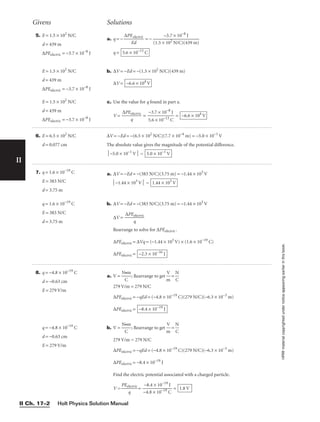


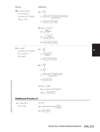
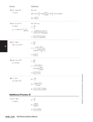
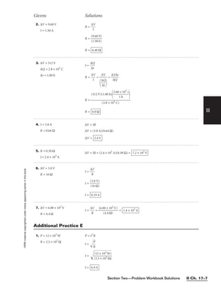


![Magnetism
Problem Workbook Solutions
II
1. B = 45 T
v = 7.5 × 10⁶
m/s
q = e = 1.60 × 10⁻¹⁹
C
me = 9.109 × 10⁻³¹
kg
Fmagnetic = qvB
Fmagnetic = (1.60 × 10⁻¹⁹
C)(7.5 × 10⁶
m/s)(45 T)
Fmagnetic = 5.4 × 10⁻¹¹
N
Additional Practice A
Givens Solutions
Copyright
©
Holt,
Rinehart
and
Winston.
All
rights
reserved.
2. q = 12 × 10−9
C
v = 450 km/h
B = 2.4 T
Fmagnetic = qvB
Fmagnetic = (12 × 10−9
C)(450 km/h)
36
1
0
h
0 s
1
1
0
k
3
m
m
(2.4 T)
Fmagnetic = 3.6 × 10⁻⁶
N
3. v = 350 km/h
q = 3.6 × 10⁻⁸
C
B = 7.0 × 10⁻⁵
T
q = 30.0°
Fmagnetic = qvB = q[v (sin q)]B
Fmagnetic = (3.6 × 10⁻⁸
C)(350 km/h)
36
1
0
h
0 s
1
1
0
k
3
m
m
(sin 30.0°)(7.0 × 10⁻⁵
T)
Fmagnetic = 1.2 × 10⁻¹⁰
N
4. v = 2.60 × 10²
km/h
Fmagnetic = 3.0 × 10⁻¹⁷
N
q = 1.60 × 10⁻¹⁹
C
Fmagnetic = qvB
B =
Fma
q
g
v
netic
B =
B = 2.6 T
(3.0 × 10⁻¹⁷
N)
(1.60 × 10⁻¹⁹ C)(2.60 × 10² km/h)
36
1
0
h
0 s
1
1
0
k
3
m
m
Section Two—Problem Workbook Solutions II Ch. 19–1](https://image.slidesharecdn.com/physicssolutions-230306125240-7bc050a7/85/physics-solutions-pdf-466-320.jpg)
![Section Two—Problem Workbook Solutions II Ch. 19–3
II
r1 =
r1 = 2.08 × 10⁻²
m
r2 =
r2 = 2.42 × 10⁻²
m
r2 − r1 = 3.40 × 10⁻³
m = 3.4 mm
(11.6 × 10⁻²⁷
kg)(2.00 × 10⁵
m/s)2
(1.92 × 10⁻¹⁴ N)
(9.98 × 10⁻²⁷
kg)(2.00 × 10⁵
m/s)2
(1.92 × 10⁻¹⁴ N)
Givens Solutions
Copyright
©
Holt,
Rinehart
and
Winston.
All
rights
reserved.
1. B = 22.5 T
l = 12 × 10−2
m
I = 8.4 × 10⁻²
A
Fmagnetic = BIl
Fmagnetic = (22.5 T)(8.4 × 10⁻²
A)(12 × 10−2
m)
Fmagnetic = 0.23 N
Additional Practice B
2. l = 1066 m
Fmagnetic = 6.3 × 10⁻²
N
I = 0.80 A
Fmagnetic = BIl
B =
B =
(0
(
.
6
8
.
0
3
A
×
)
1
(1
0
0
−
6
2
6
N
m
)
)
B = 7.4 × 10⁻⁵
T
Fmagnetic
Il
3. l = 5376 m
Fmagnetic = 3.1 N
I = 12 A
q = 38°
Fmagnetic = BIl = [B(sin q)]Il
B =
B =
B = 7.8 × 10⁻⁵
T
(3.1 N)
(12 A)(5376 m)(sin 38.0°)
Fmagnetic
Il(sin q)
4. l = 21.0 × 10³
m
B = 6.40 × 10⁻⁷
T
Fmagnetic = 1.80 × 10⁻²
N
Fmagnetic = BIl
I =
I =
I = 1.34 A
(1.80 × 10⁻²
N)
(6.40 × 10⁻⁷ T)(21.0 × 10³ m)
Fmagnetic
Bl](https://image.slidesharecdn.com/physicssolutions-230306125240-7bc050a7/85/physics-solutions-pdf-468-320.jpg)
![Holt Physics Solution Manual
II Ch. 19–4
II
5. B = 2.5 × 10⁻⁴
T
l = 4.5 × 10⁻²
m
Fmagnetic = 3.6 × 10⁻⁷
N
Fmagnetic = BIl
I =
I =
I = 3.2 10–2
A
(3.6 × 10⁻⁷
N)
(2.5 × 10⁻⁴ T)(4.5 × 10⁻² m)
Fmagnetic
Bl
Givens Solutions
Copyright
©
Holt,
Rinehart
and
Winston.
All
rights
reserved.
6. Fmagnetic = 5.0 × 10⁵
N
B = 3.8 T
I = 2.00 × 10²
A
Fmagnetic = BIl
l =
Fma
B
g
I
netic
l =
l = 6.6 × 10²
m
(5.0 × 10⁵
N)
(3.8 T)(2.00 × 10² A)
7. Fmagnetic = 16.1 N
B = 6.4 × 10⁻⁵
T
I = 2.8 A
Fmagnetic = BIl
l =
Fma
B
g
I
netic
l =
l = 9.0 × 10⁴
m
(16.1 N)
(6.4 × 10⁻⁵ T)(2.8 A)
8. B = 0.040 T
I = 0.10 A
q = 45°
l = 55 cm 0.55 m
Fmagnetic = BIl = [B(sin q)]Il
Fmagnetic = (0.040 T)(sin 45°)(0.10 A)(0.55 m)
Fmagnetic = 1.6 × 10⁻³
Ν
9. B = 38 T
l = 2.0 m
m = 75 kg
g = 9.81 m/s2
Fmagnetic = BIl
Fg = mg
Fmagnetic = Fg
BIl = mg
I =
I =
(75
(3
k
8
g
T
)(
)
9
(
.
2
8
.
1
0
m
m
/
)
s2
)
I = 9.7 A
mg
Bl](https://image.slidesharecdn.com/physicssolutions-230306125240-7bc050a7/85/physics-solutions-pdf-469-320.jpg)
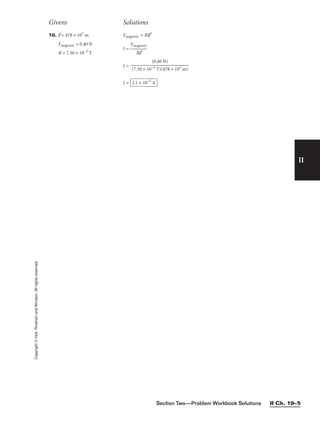

![II
Copyright
©
Holt,
Rinehart
and
Winston.
All
rights
reserved.
Section Two—Problem Workbook Solutions II Ch. 20–1
1. Ai = 6.04 × 10⁵
m2
Af =
1
2
(6.04 × 10⁵
m2
)
B = 6.0 × 10⁻⁵
T
emf = 0.80 V
N = 1 turn
q = 0.0°
emf = −N =
∆t = ∆A
∆t = (Af − Ai)
∆t = (6.04 × 10⁵
m2
)
1
2
− 1
∆t = 23 s
−(1)(6.0 × 10⁻⁵
T)(cos 0.0°)
(0.80 V)
−NB cos q
emf
−NB cos q
emf
−N∆[AB cos q]
∆t
∆ΦM
∆t
Additional Practice A
Givens Solutions
4. Af = 3.2 × 10⁴
m2
Ai = 0.0 m2
∆t = 20.0 min
B = 4.0 × 10⁻²
T
N = 300 turns
q = 0.0°
emf = −N = = −NB cos q = (Af − Ai)
emf = [(3.2 × 10⁴
m2
) − (0.0 m2
)]
emf = −3.2 × 10²
V
−(300)(4.0 × 10⁻²
T)(cos 0.0°)
(20.0 min)
1
6
m
0
i
s
n
−NB cos q
∆t
∆A
∆t
−N∆[AB cos q]
∆t
∆ΦM
∆t
2. r =
100
2
.0 m
= 50.0 m
Bi = 0.800 T
Bf = 0.000 T
q = 0.00°
emf = 46.7 V
N = 1 turn
emf = −N =
∆t = −NA cos q =
∆t =
∆t = 135 s
−(1)(p)(50.0 m)2
(cos 0.0°)(0.000 T − 0.800 T)
(46.7 V)
−N(pr2
)(cos q)(Bf − Bi)
emf
∆B
emf
−N∆[AB cos q]
∆t
∆ΦM
∆t
Electromagnetic
Induction
Problem Workbook Solutions
3. emf = 32.0 × 10⁶
V
Bi = 1.00 × 10³
T
Bf = 0.00 T
A = 4.00 × 10⁻²
m2
N = 50 turns
q = 0.00°
emf = −N =
∆t = −NA cos q =
∆t =
∆t = 6.3 × 10⁻⁵
s
−(50)(4.00 × 10⁻²
m2
)(cos 0.00°)[(0.00 T) − (1.00 × 10³
T)]
(32.0 × 10⁶ V)
−NAcos q(Bf − Bi)
emf
∆B
emf
−N∆[AB cos q]
∆t
∆ΦM
∆t](https://image.slidesharecdn.com/physicssolutions-230306125240-7bc050a7/85/physics-solutions-pdf-472-320.jpg)
![II
Copyright
©
Holt,
Rinehart
and
Winston.
All
rights
reserved.
Holt Physics Solution Manual
II Ch. 20–2
5. Bi = 8.0 × 10⁻¹⁵
T
Bf = 10 Bi = 8.0 × 10⁻¹⁴
T
∆t = 3.0 × 10⁻²
s
A = 1.00 m2
emf = −1.92 × 10⁻¹¹
V
q = 0.0°
emf = −N =
N = =
N =
N = 8 turns
−(−1.92 × 10⁻¹¹
V)(3.0 × 10⁻²
s)
(1.00 m2)(cos 0.0°)[(8.0 × 10⁻¹⁴ T) − (8.0 × 10⁻¹⁵ T)]
−(emf)(∆t)
A cos q(Bf − Bi)
−(emf)(∆t)
A cos q ∆B
−N∆[AB cos q]
∆t
∆ΦM
∆t
6. Bi = 0.50 T
Bf = 0.00 T
N = 880 turns
∆t = 12 s
emf = 147 V
q = 0.0°
emf = −N = = −NA cos q
∆
∆
B
t
A = =
A =
A = 4.0 m2
−(147 V)(12 s)
(880)(cos 0.0°)(0.00 T − 0.50 T)
−(emf)(∆t)
N cos q (Bf − Bi)
−(emf)(∆t)
N cos q ∆B
−N∆[AB cos q]
∆t
ΦM
∆t
Givens Solutions
1. ∆Vrms = 120 V
R = 6.0 × 10⁻²
Ω
= 0.707
1
2
a. Irms =
∆V
R
rms
Irms =
(6.0
(1
×
2
1
0
0
V
−2
)
Ω)
Irms =
b. Imax = (Irms)
2
Imax =
(2.0
(0
×
.7
1
0
0
7
3
)
A)
Imax =
c. P = (Irms)(∆Vrms)
P = (2.0 × 10³
A)(120 V)
P = 2.4 × 10⁵
W
2.8 × 10³
A
2.0 × 10³
A
Additional Practice B](https://image.slidesharecdn.com/physicssolutions-230306125240-7bc050a7/85/physics-solutions-pdf-473-320.jpg)

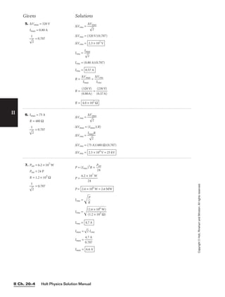

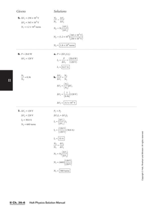
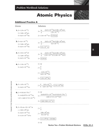
![II
Copyright
©
Holt,
Rinehart
and
Winston.
All
rights
reserved.
Holt Physics Solution Manual
II Ch. 21–2
Givens Solutions
8. v = 1.80 × 10⁻¹⁷
m/s
∆t = 1.00 year
l = ∆x
c = 3.00 × 10⁸
m/s
h = 6.63 × 10⁻³⁴
J•s
∆x = v∆t
∆x = (1.80 × 10⁻¹⁷
m/s)(1.00 year)
365
1
.2
y
5
ea
d
r
ays
1
24
da
h
y
36
1
0
h
0 s
∆x =
E = hf =
h
l
c
=
∆
h
x
c
E =
E = 3.50 × 10⁻¹⁶
J
(6.63 × 10⁻³⁴
J•s)(3.00 × 10⁸
m/s)
5.68 × 10⁻¹⁰
m
5.68 × 10⁻¹⁰
m
E = (6.63 × 10⁻³⁴
J•s)(3.3 × 10⁸
Hz)
E =
E = (4.14 × 10⁻¹⁵
eV•s)(3.3 × 10⁸
Hz)
E = 1.4 × 10⁻⁶
eV
2.2 × 10⁻²⁵
J
Additional Practice B
1. hft = 4.5 eV
KEmax = 3.8 eV
h = 4.14 × 10⁻¹⁵
eV•s
f =
[KEma
h
x + hft]
=
4
[3
.1
.8
4
e
×
V
10
+
−
4
1
.
5
5
e
e
V
V
•
]
s
= 2.0 × 10¹⁵
Hz
2. hft = 4.3 eV
KEmax = 3.2 eV
h = 4.14 × 10⁻¹⁵
eV•s
KEmax = hf − hft
f =
KEma
h
x + hft
f =
4.
3
1
.
4
2
×
eV
10
+
−
4
15
.3
e
e
V
V
•s
f = 1.8 × 10¹⁵
Hz
3. hft,Cs = 2.14 eV
hft,Se = 5.9 eV
h = 4.14 × 10⁻¹⁵
eV•s
c = 3.00 × 10⁸
m/s
KEmax = 0.0 eV for both
cases
a. KEmax = hf − hft = 0.0 eV =
h
l
c
− hft
l =
h
h
f
c
t
lCs =
hf
h
t,
c
Cs
=
lCs =
b. lSe =
hf
h
t,
c
Se
=
lSe = 2.1 × 10⁻⁷
m = 2.1 × 10²
nm
(4.14 × 10⁻¹⁵
eV•s)(3.00 × 10⁸
m/s)
5.9 eV
5.80 × 10⁻⁷
m = 5.80 × 10²
nm
(4.14 × 10⁻¹⁵
eV•s)(3.00 × 10⁸
m/s)
2.14 eV](https://image.slidesharecdn.com/physicssolutions-230306125240-7bc050a7/85/physics-solutions-pdf-479-320.jpg)
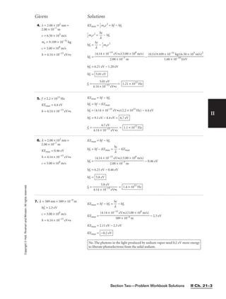
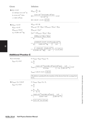


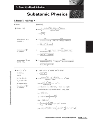
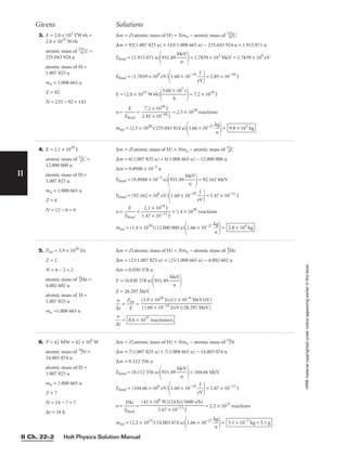


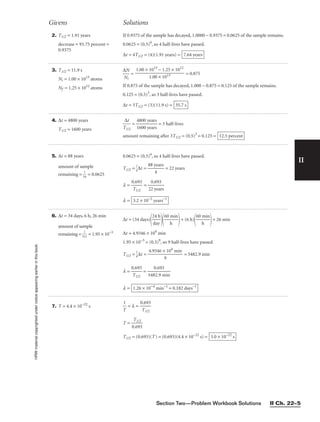

![Section Two—Problem Workbook Solutions Appendix J–1
Appendix J
Advanced Topics
II
1. r = 10.0 km
∆q = +15.0 rad
∆s = r∆q = (10.0 km)(15.0 rad) =
The particle moves in the positive, or , direction around the
neutron star’s “north” pole.
counterclockwise
1.50 × 10²
km
Additional Practice A
Givens Solutions
Copyright
©
by
Holt,
Rinehart
and
Winston.
All
rights
reserved.
2. ∆q = 3(2p rad)
r = 6560 km
∆s = r∆q = (6560 km)[(3)(2p rad)] = 1.24 × 10⁵
km
3. r =
1.40 ×
2
105
km
= 7.00 × 10⁴
km
∆q = 1.72 rad
rE = 6.37 × 10³
km
a. ∆s = r∆q = (7.00 × 10⁴
km)(1.72 rad) =
b. ∆qE =
∆
rE
s
= = 3.00 rev, or 3.00 orbits
(1.20 × 10⁵
km)(1 rev/2p rad)
6.37 × 10³
km
1.20 × 10⁵
km
4. ∆q = 225 rad
∆s = 1.50 × 10⁶
km
r =
∆
∆
q
s
=
1.50
22
×
5
1
r
0
a
6
d
km
= 6.67 × 10³
km
5. r = 5.8 × 10⁷
km
∆s = 1.5 × 10⁸
km
∆q =
∆
r
s
=
1
5
.
.
5
8
×
×
1
1
0
0
8
7
k
k
m
m
= 2.6 rad
6. ∆s = −1.79 × 10⁴
km
r = 6.37 × 10³
km
∆q =
∆
r
s
=
−
6
1
.3
.7
7
9
×
×
1
1
0
0
3
4
k
k
m
m
= −2.81 rad
Additional Practice B
1. r = 1.82 m
wavg = 1.00 × 10⁻¹
rad/s
∆t = 60.0 s
∆q = wavg∆t = (1.00 × 10⁻¹
rad/s)(60.0 s) =
∆s = r∆q = (1.82 m)(6.00 rad) = 10.9 m
6.00 rad
2. ∆t = 120 s
wavg = 0.40 rad/s
∆q = wavg∆t = (0.40 rad/s)(120 s) = 48 rad
3. r = 30.0 m
∆s = 5.0 × 10²
m
∆t = 120 s
wavg =
∆
∆
q
t
=
r
∆
∆
s
t
=
(3
5
0
.
.
0
0
×
m
1
)(
0
1
2
2
m
0 s)
= 0.14 rad/s](https://image.slidesharecdn.com/physicssolutions-230306125240-7bc050a7/85/physics-solutions-pdf-490-320.jpg)
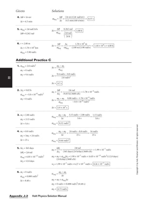
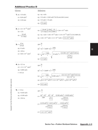
![II
Givens Solutions
Copyright
©
by
Holt,
Rinehart
and
Winston.
All
rights
reserved.
6. r = 1.0 km
wi = 5.0 × 10⁻³
rad/s
∆t = 14.0 min
∆q = 2p rad
∆q = wi∆t +
1
2
a∆t2
a =
2(∆q
∆
−
t2
wi∆t)
=
a = = = 6.0 × 10⁻⁶
rad/s2
(2)(2.1 rad)
[(14.0 min)(60 s/min)]2
(2)(6.3 rad − 4.2 rad)
[(14.0 min)(60 s/min)]2
(2)[2p rad − (5.0 × 10⁻³
rad/s)(14.0 min)(60 s/min)]
[(14.0 min)(60 s/min)]2
7. wi = 7.20 × 10⁻²
rad/s
∆q = 12.6 rad
∆t = 4 min, 22 s
∆t = (4 min)(60 s/min) + 22 s = 262 s
∆q = wi∆t +
1
2
a∆t2
a =
2(∆q
∆
−
t2
wi∆t)
=
a = =
(2)(
(
−
2
6
6
.
2
3
s
r
)
a
2
d/s)
= −1.8 × 10⁻⁴
rad/s2
(2)(12.6 rad − 18.9 rad)
(262 s)2
(2)[12.6 rad − (7.20 × 10⁻²
rad/s)(262 s)]
(262 s)2
8. wi = 27.0 rad/s
wf = 32.0 rad/s
∆t = 6.83 s
aavg =
wf
∆
−
t
wi
= =
5.
6
0
.8
r
3
ad
s
/s
aavg = 0.73 rad/s2
32.0 rad/s − 27.0 rad/s
6.83 s
9. a = 2.68 × 10⁻⁵
rad/s2
∆t = 120.0 s
wi =
2p
1
r
2
ad
∆q = wi∆t +
1
2
a∆t2
∆q =
2
1
p
2
r
h
ad
(1 h/3600 s)(120.0 s) +
1
2
(2.68 × 10⁻⁵
rad/s2
)(120.0 s)2
∆q = 1.7 × 10⁻²
rad + 1.93 × 10⁻¹
rad = 0.210 rad
10. wi = 6.0 × 10⁻³
rad/s
wf = 3wi = 18 × 10−3
rad/s
a = 2.5 × 10⁻⁴
rad/s2
∆q =
wf
2
2
−
a
wi
2
∆q = =
∆q = = 0.56 rad
2.8 × 10⁻⁴
rad2
/s2
5.0 × 10⁻⁴
rad/s2
3.2 × 10⁻⁴
rad2
/s2
− 3.6 × 10⁻⁵
rad2
/s2
(2)(2.5 × 10⁻⁴
rad/s2
)
(18 × 10−3
rad/s)2
− (6.0 × 10⁻³
rad/s)2
(2)(2.5 × 10⁻⁴
rad/s2
)
11. wi = 9.0 × 10⁻⁷
rad/s
wf = 5.0 × 10⁻⁶
rad/s
a = 7.5 × 10⁻¹⁰
rad/s2
∆t =
wf
a
− wi
∆t = =
∆t = 5.5 × 10³
s = 1.5 h
4.1 × 10⁻⁶
rad/s
7.5 × 10⁻¹⁰ rad/s2
5.0 × 10⁻⁶
rad/s − 9.0 × 10⁻⁷
rad/s
7.5 × 10⁻¹⁰ rad/s2
Holt Physics Solution Manual
Appendix J–4](https://image.slidesharecdn.com/physicssolutions-230306125240-7bc050a7/85/physics-solutions-pdf-493-320.jpg)

![II
Givens Solutions
Copyright
©
by
Holt,
Rinehart
and
Winston.
All
rights
reserved.
1. r = 32 m
at = 0.20 m/s2
a =
a
r
t
=
0.2
3
0
2
m
m
/s2
a = 6.2 × 10⁻³
rad/s2
Additional Practice F
2. r = 8.0 m
at = −1.44 m/s2
a =
a
r
t
=
−1.
8
4
.
4
0
m
m
/s2
= −0.18 rad/s2
3. ∆w = −2.4 × 10⁻²
rad/s
∆t = 6.0 s
at = − 0.16 m/s2
a =
∆
∆
w
t
=
−2.4 ×
6
1
.0
0−
s
2
rad/s
= −4.0 × 10⁻³
rad/s2
r =
a
a
t
=
−4.0
−0
×
.1
1
6
0−
m
3
/
r
s
a
2
d/s2
= 4.0 × 101
m
4. ∆q′ = 14 628 turns
∆t′ = 1.000 h
at = 33.0 m/s2
wi = 0 rad/s
∆q = 2p rad
r =
a
a
t
a =
wf
2
2∆
−
q
wi
2
wf =
r = =
r =
2
− (0 rad/s)2
= 0.636 m
(14 628 turns)(2p rad/turn)
(1.000 h)(3600 s/h)
2at∆q
∆
∆
q
t′
′
2
− wi
2
∆
∆
q
t′
′
2
− wi
2
2∆q
∆q′
∆t′
5. r = 56.24 m
wi = 6.00 rad/s
wf = 6.30 rad/s
∆t = 0.60 s
at = ra
a =
wf
∆
−
t
wi
at = r
wf
∆
−
t
wi
= (56.24 m)
=
at = 28 m/s2
(56.24 m)(0.30 rad/s)
0.60 s
6.30 rad/s − 6.00 rad/s
0.60 s
at
(2)(33.0 m/s2
)(2p rad)
6. r = 1.3 m
∆q = 2p rad
∆t = 1.8 s
wi = 0 rad/s
at = ra
α =
2(∆q
∆
−
t2
wi∆t)
at = r
2(∆q
∆
−
t2
wi∆t)
= (1.3 m)
at = 5.0 m/s2
(2)[2p rad − (0 rad/s)(1.8 s)]
(1.8 s)2
Holt Physics Solution Manual
Appendix J–6](https://image.slidesharecdn.com/physicssolutions-230306125240-7bc050a7/85/physics-solutions-pdf-495-320.jpg)

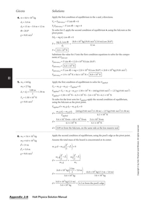

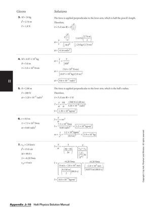


![II
Copyright
©
by
Holt,
Rinehart
and
Winston.
All
rights
reserved. 4. vi = 395 km/h
ri = 1.20 × 10²
m
∆
∆
r
t
= 0.79 m/s
∆t = 33 s
rf = ri −
∆
∆
r
t
∆t
Li = Lf
Ii wi = Lf wf
mri
2
v
ri
i
= mrf
2
v
rf
f
ri vi = rf vf =
ri −
∆
∆
r
t
∆t
vf
vf = =
vf = =
vf = 5.0 × 10²
km/h
(1.20 × 10²
m)(395 km/h)
94 m
(1.20 × 10²
m)(395 km/h)
1.20 × 10²
m − 26 m
(1.20 × 10²
m)(395 km/h)
1.20 × 10²
− (0.79 m/s)(33 s)
ri vi
[ri −
∆
∆
r
t
∆t]
Givens Solutions
5. ri =
10.
2
0 m
= 5.00 m
rf =
4.0
2
0 m
= 2.00 m
wi = 1.26 rad/s
Li = Lf
Iiwi = Ifwf
mri
2
wi = mrf
2
wf
wf =
ri
r
2
f
w
2
i
=
wf = 7.88 rad/s
(5.00 m)2
(1.26 rad/s)
(2.00 m)2
6. R = 3.00 m
M = 1.68 × 10⁴
kg
ri = 2.50 m
rf = 3.00 m
m = 2.00 × 10²
kg
wi = 3.46 rad/s
Li = Lf
Iiwi = Ifwf
2
1
MR2
+ mri
2
wi =
1
2
MR2
+ mrf
2
wf
wf =
wf =
2
1
(1.68 × 10⁴
kg)(3.00 m)2
+ (2.00 × 10²
kg)(2.50 m)2
(3.46 rad/s)
2
1
(1.68 × 10⁴
kg)(3.00 m)2 + (2.00 × 10² kg)(3.00 m)2
wf =
wf =
wf = 3.43 rad/s
∆w = wf − wi = 3.43 rad/s − 3.46 rad/s = −0.03 rad/s
The angular speed decreases by 0.03 rad/s.
(7.68 × 10⁴
kg•m2
)(3.46 rad/s)
7.74 × 10⁴
kg•m2
(7.56 × 10⁴
kg•m2
+ 1.25 × 10³
kg•m2
)(3.46 rad/s)
7.56 × 10⁴
kg•m2
+ 1.80 × 10³
kg•m2
2
1
MR2
+ mri
2
wi
1
2
MR2
+ mrf
2
Section Two—Problem Workbook Solutions Appendix J–13](https://image.slidesharecdn.com/physicssolutions-230306125240-7bc050a7/85/physics-solutions-pdf-502-320.jpg)
![1. m = 407 kg
h = 57.0 m
vf = 12.4 m/s
wf = 28.0 rad/s
g = 9.81 m/s2
MEi = MEf
mgh =
1
2
mvf
2
+
1
2
I wf
2
1
2
I wf
2
= mgh −
1
2
mvf
2
I =
2mgh
w
−
f
2
mvf
2
=
m(2g
w
h
f
2
− vf
2
)
I =
I = =
I = 5.0 × 10²
kg•m2
(407 kg)(9.7 × 10²
m2
/s2
)
(28.0 rad/s)2
(407 kg)(1.12 × 10³
m2
/s2
− 154 m2
/s2
)
(28.0 rad/s)2
(407 kg)[(2)(9.81 m/s2
)(57.0 m) − (12.4 m/s)2
]
(28.0 rad/s)2
Givens Solutions
II
Copyright
©
by
Holt,
Rinehart
and
Winston.
All
rights
reserved.
Additonal Practice J
2. h = 5.0 m
g = 9.81 m/s2
MEi = MEf
mgh =
1
2
mvf
2
+
2
1
Iwf
2
mgh =
1
2
mvf
2
+
1
2
(mr2
)
v
r
f
2
2
mgh = mvf
2
1
2
+
1
2
= mvf
2
vf =
gh
=
(9
.8
1
m
/s
2)
(5
.0
m
)
vf = the mass is not required
7.0 m/s
3. h = 1.2 m
g = 9.81 m/s2
MEi = MEf
1
2
mvi
2
+
1
2
Iwi
2
= mgh
2
1
mvi
2
+
1
2
1
2
mr2
v
r
i
2
2
= mgh
mvi
2
1
2
+
1
4
=
3
4
mvi
2
= mgh
vi =
4
3
g
h
= = 4.0 m/s
(4)(9.81 m/s2
)(1.2 m)
3
4. vf = 12.0 m/s
I = 0.80mr2
g = 9.81 m/s2
MEi = MEf
mgh =
2
1
mvf
2
+
2
1
Iwf
2
=
2
1
mvf
2
+
2
1
(0.80 mr2
)
v
r
f
2
mgh = mvf
2
2
1
+
0.
2
80
= 0.90 mvf
2
h =
0.90
g
vf
2
=
(0.9
9
0
.
)
8
(
1
12
m
.0
/s
m
2
/s)2
h = 13 m
Holt Physics Solution Manual
Appendix J–14](https://image.slidesharecdn.com/physicssolutions-230306125240-7bc050a7/85/physics-solutions-pdf-503-320.jpg)
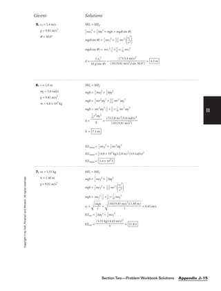
![II
Copyright
©
by
Holt,
Rinehart
and
Winston.
All
rights
reserved.
1. P1 = (1 + 0.12)P2 = 1.12 P2
v1 = 0.60 m/s
v2 = 4.80 m/s
ρ = 1.00 × 10³
kg/m3
h1 = h2
P1 +
1
2
ρv1
2
+ ρgh1 = P2 +
1
2
ρv2
2
+ ρgh2
h1 = h2, and P2 =
1
P
.1
1
2
, so the equation simplifies to
P1 +
1
2
ρv1
2
=
1
P
.1
1
2
+
1
2
ρv2
2
P11 −
1.
1
12
=
1
2
ρ(v2
2
− v1
2
)
P1 = =
P1 =
P1 = = 1.06 × 10⁵
Pa
(1.00 × 10³
kg/m3
)(22.6 m2
/s2
)
(2)(0.107)
(1.00 × 10³
kg/m3
)(23.0 m2
/s2
− 0.36 m2
/s2
)
(2)(1 − 0.893)
(1.00 × 10³
kg/m3
)[(4.80 m/s)2
− (0.60 m/s)2
]
(2)
1 −
1.
1
12
ρ(v2
2
− v1
2
)
(2)
1 −
1.
1
12
Additional Practice K
Givens Solutions
2. r1 =
4.1
2
0 m
= 2.05 m
v1 = 3.0 m/s
r2 =
2.7
2
0 m
= 1.35 m
P2 = 82 kPa
ρ = 1.00 × 10³
kg/m3
h1 = h2
A1v1 = A2v2
v2 =
A
A
1v
2
1
=
π
π
r1
r
2
2
v
2
1
=
r1
r2
2
2
v1
v2 = = 6.9 m/s
P1 +
1
2
rv1
2
+ ρgh1 = P2 +
1
2
rv2
2
+ ρgh2
h1 = h2, so the equation simplifies to
P1 +
2
1
rv1
2
= P2 +
2
1
rv2
2
P1 = P2 +
2
1
r(v2
2
− v1
2
)
P1 = 82 × 103
Pa +
2
1
(1.00 × 10³
kg/m3
)[(6.9 m/s)2
− (3.0 m/s)2
]
P1 = 82 × 103
Pa +
2
1
(1.00 × 10³
kg/m3
)(48 m2
/s2
− 9.0 m2
s2
)
P1 = 82 × 103
Pa +
2
1
(1.00 × 10³
kg/m3
)(39 m2
/s2
)
P1 = 82 × 103
Pa + 2.0 × 10⁴
Pa = 10.2 × 10⁴
Pa = 102 kPa
(2.05 m)2
(3.0 m/s)
(1.35 m)2
3. h2 − h1 =
1
2
h
∆x = 19.7 m
To find the horizontal speed of the cider, recall that for a projectile with no initial
vertical speed,
∆x = v∆t
∆y = −
1
2
g ∆t2
= −
1
2
h
∆t =
h
g
v =
∆
∆
x
t
= =
g
∆
h
x2
P1 +
1
2
ρv1
2
+ ρgh1 = P2 +
1
2
ρv2
2
+ ρgh2
∆x
h
g
Holt Physics Solution Manual
Appendix J–16](https://image.slidesharecdn.com/physicssolutions-230306125240-7bc050a7/85/physics-solutions-pdf-505-320.jpg)

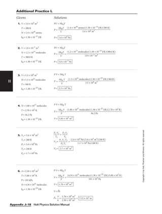

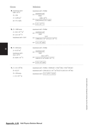

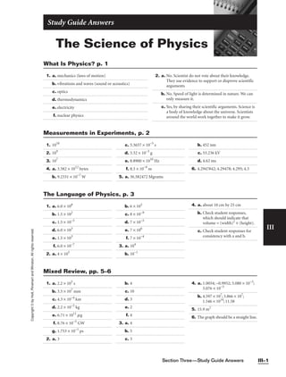
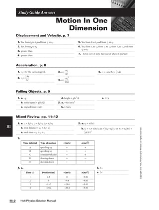
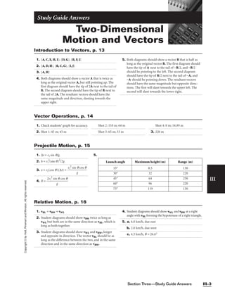


![Polymer [ बहुलक ] Chemistry Notes PDF - Irfanullah Mehar - JJ Sir Chemistry.pdf](https://cdn.slidesharecdn.com/ss_thumbnails/polymerchemistrynotespdf-irfanullahmehar-jjsirchemistry-260210172118-3f9b37f7-thumbnail.jpg?width=640&height=640&fit=bounds)


