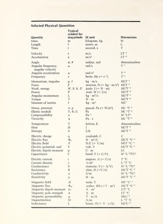
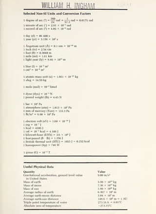
This document provides a summary of selected physical quantities including their typical symbols, SI units, and dimensions. It lists quantities such as mass, length, time, velocity, acceleration, angle, angular frequency, momentum, force, work, power, stress, elastic moduli, temperature, heat, entropy, electric charge, electric field, electric potential, capacitance, current, resistance, magnetic field, and inductance among others. It also provides conversion factors between common non-SI units and the International System of Units.


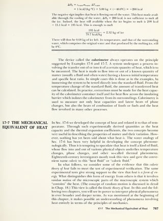
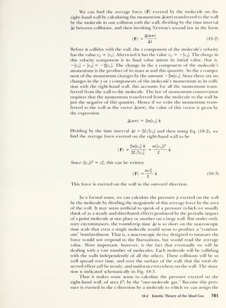
![The strain e is the change in length A/ of a sample per unit of undistorted length l of
the sample; the quantities A/ and / are shown in Fig. 16-1. Since strain is the
quotient of two lengths, it is a dimensionless number. The quantity A/ is a
signed scalar which is defined so that its value is positive when the sample is
stretched and negative when it is compressed. Since the length l of the
sample is always positive, the value of the strain e is positive for stretch and
negative for compression.
To see that the strain is a quantity which is indeed independent of the length
of the sample on which it is measured, consider again the system of two identical
springs linked end to end. If each spring has length], the two together have length
21. If each spring stretches an amount AJ, the two together stretch by an amount
2A1. Thus the strain of each spring individually is given by e = AI /l. The strain of
the two taken together is given by e' = 2 AJ/21 = e.
Now that we have defined a quantity, strain, which is independent of
the length of the sample, we develop a definition of a quantity which is
independent of its thickness. Example 16-1 investigates the effect of
thickness by considering two identical rods mounted side by side.
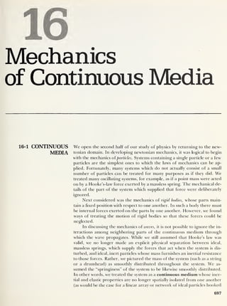
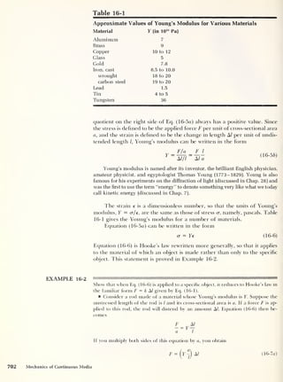
EXAMPLE 16-1
Positive
x direction
F
*
Fig. 16-2 Illustration for Example 16-1.
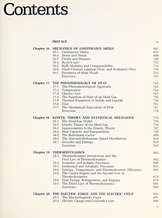
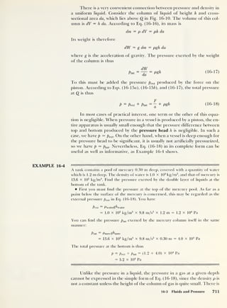
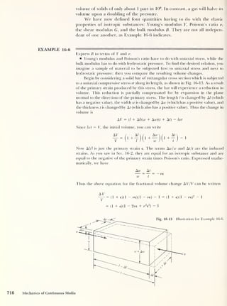
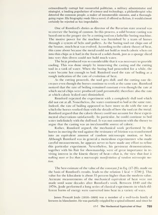
Two identical steel rods, each having a square cross section of area Aa and a force
constant k, are arranged side by side in the apparatus shown in Fig. 16-2. (The as-
sumption of a square cross section is for simplicity only and does not affect the con-
clusions.) Find the effective force constant k" of the pair. Then let the force constant
k for each rod be k = 2 X 10
7
N/m, and find the force constant required to stretch
the pair of rods 1 mm.
The symmetry of the apparatus is such that the force applied to the crossbar at
a point midway between the rods must be balanced by two opposite forces, each of
magnitude F/2, exerted by the two rods. According to Hooke’s law, each rod will
therefore stretch by an amount Al" given by the equation
F 1 F
But the whole system stretches by the same amount as either rod, and the force ap-
plied to the whole system is F. When you insert these whole-system values into
Hooke’s law, you obtain
F
Al"
F
F/ 2k
or
k" = 2k
Since the force constant is a measure of stiffness, it is not surprising that two iden-
tical rods tied together in parallel, as shown, and sharing the external load are twice
as stiff as either rod alone.
You can now find the force required to stretch the system an amount A/" =
A/ = 1 mm. Since k = 2 x 10
7
N/m, you have for the pair of rods
k" = 2 X 2 x 10
7
N/m = 4 x 10
7
N/m
Hooke’s law thus gives you
F = k" M" = 4 x 10
7
N/m x 1 x 10“3
m = 4 x 10
4
N
700 Mechanics of Continuous Media](https://image.slidesharecdn.com/robertm-220626164724-d75ac43b/85/Robert-M-Eisberg-Lawrence-S-Lerner-Physics_-Foundations-and-Appli-pdf-24-320.jpg?cb=1675858377)
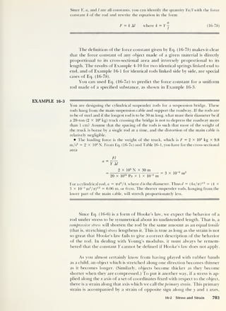
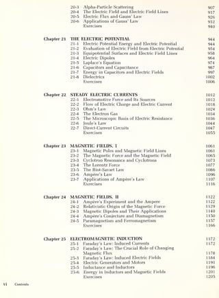
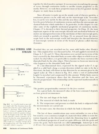
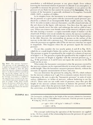
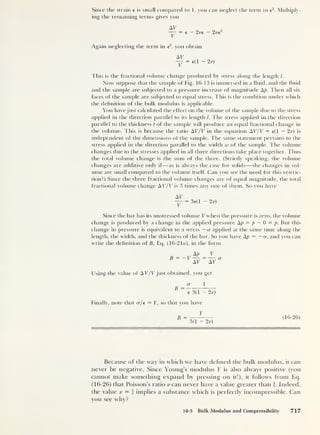
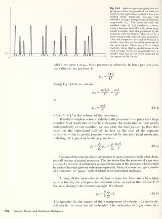
![which we call the induced strain. The phenomenon is illustrated in Fig. 16-5.
F
Fig. 16-5 When a rod is stretched, it
becomes thinner. Here the applied stress
results in a positive primary strain
and negative induced strains.
We can account qualitatively for this phenomenon on the microscopic level.
In an isotropic substance [one whose macroscopic properties are the same in all
directions), every atom lies equidistant, on the average, from its nearest
neighbors. This is the position in which all the attractive and repulsive forces
between it and neighboring atoms balance. In Fig. 16-6 are shown two neighboring
atoms A andB, lying along thex direction. When a tensile stress is applied along
the x axis, the average interatomic distance along that direction increases as the
sample stretches. As A and B separate, their neighbors C and D tend to move
toward the axis joining A and B —that is, the stress axis. This displacement of C
and D reduces the average interatomic distance toward the undisturbed value. The
result in the large is a reduction in the dimensions of the sample in the plane
normal to the direction of stress. In similar manner, a compressive stress along the
x axis and its accompanying negative strain will result in an expansion of the
sample in the yz plane normal to the axis of stress.
A uniaxial stress always leads to a change in the volume of the sample.
That is, the strain induced in the plane normal to the applied stress (which
contains C and D in Fig. 1 6-6) is never sufficient to make up for the primary
strain along the stress axis (along which A and B lie in the same figure).
In an isotropic substance the induced strain is the same in all directions
in the plane normal to the primary strain. The ratio of the induced strain to
the primary strain is called Poissons ratio [after the French mathematician
and physicist Simon Poisson (1781-1840)]. Poisson’s ratio is expressed
mathematically as follows. Suppose that a stress is applied lengthwise to a
sample of length /, width w, and thickness t. As a result, the length changes
by an amount A/, while the width and thickness change, respectively, by
amounts Arc and At, whose values are of opposite sign to that of A/. The pri-
mary strain is then given by the ratio A///, while the induced strain has a
value given by either the ratio Aw/w or the ratio At/t, which have equal val-
ues. Poisson’s ratio v is then defined by the equation
Aw/w At/t
A///
=
“ATfl
(16-8)
A
• D
r
Ax
Fig. 16-6 Idealized microscopic picture of the pro-
cess shown in Fig. 16-5. Atoms A, B. C, and D are
equidistant in the unstressed isotropic sample. Stress
applied along the x axis separates A and B. Atoms
C and D move to new equilibrium positions closer to
one another, in such a way as to reduce the change in
the average interatomic distance produced by the
applied stress.
Av
D
I
704 Mechanics of Continuous Media](https://image.slidesharecdn.com/robertm-220626164724-d75ac43b/85/Robert-M-Eisberg-Lawrence-S-Lerner-Physics_-Foundations-and-Appli-pdf-28-320.jpg?cb=1675858377)
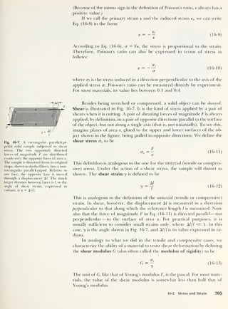
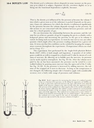
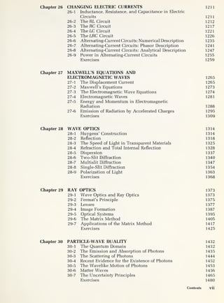
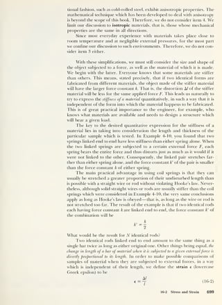
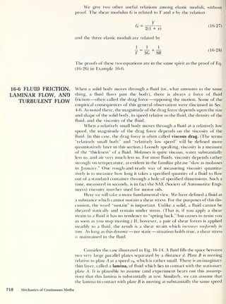
![Table 16-2
Bulk Modulus for Typical Solids andI Liquids
Substance B (in Pa)
Aluminum 7.46 X 10¹⁰
Brass 10.7 X 10¹⁰
Copper 13.1 X 10¹⁰
Glass 1.4 X 10¹⁰
Steel 18 X 1010
Lead 5.0 X 10¹⁰
Diamond 20 X 1010
Ethanol (grain alcohol) 0.9 X 10⁹
Glycerine 4.6 X 10⁹
Mercury 27.0 X 10⁹
Water (20°C) 2.06 X 10⁹
For gases, the bulk modulus can be deduced directly from Boyle’s law.
From Ec]. (16-206) we have
P=^ (16-22)
where c is some constant. If the pressure is changed by an infinitesimal
amount dp, the corresponding change in the volume can he found by dif-
ferentiating both sides of this equation with respect to V, to obtain
dp c
~dV
= ~
V*
(16-23)
Substituting this value of dp/dV into the definition of B, Eq. (16-216), we
obtain
Comparing this with Eq. (16-22) gives the final result
B = p for constant temperature (16-24)
Thus/or a gas, the bulk modulus is just equal to the pressure. The limitations on
the applicability of this equation are the same as the limitations on Boyle’s
law. Generally speaking, it is accurate if the pressure is not too high and the
temperature is not too low. It is quite accurate for familiar gases such as
oxygen and nitrogen near atmospheric pressure and room temperature.
Particularly in the case of gases, it is often more convenient to speak in
terms of the susceptibility to compression rather than the resistance to com-
pression. For this purpose, we define the compressibility k (lowercase
Greek kappa) to be the reciprocal of the bulk modulus. That is,
1 _
B
~ ~ V ~dp
(16-25)
The compressibility of solids is of the order of 10
-11
Pa
-1
. In other
words, an increase in pressure of 1 Pa results in a reduction in volume of
about 1 part in 1011
. In terms of commonly encountered pressures, a
doubling of the pressure from 1 atm to 2 atm results in a reduction in the
16-5 Bulk Modulus and Compressibility 715](https://image.slidesharecdn.com/robertm-220626164724-d75ac43b/85/Robert-M-Eisberg-Lawrence-S-Lerner-Physics_-Foundations-and-Appli-pdf-39-320.jpg?cb=1675858377)
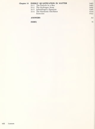
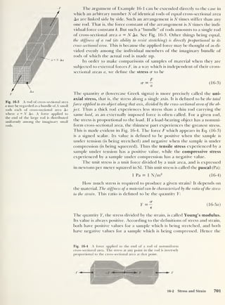
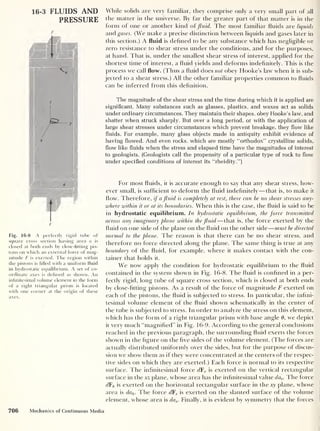
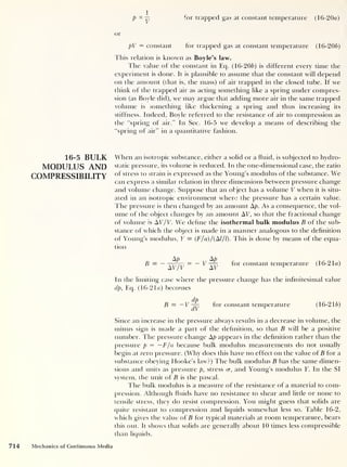
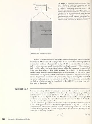
![Plate B
b
a
Plate A
i f
2
Fig. 16-14 Viscous drag in an idealized system. Two very
large parallel plates A and B are separated by a distance d.
The space between them is filled with fluid. A constant
force F must be applied to plate B to keep it moving at a
constant speed v0 with respect to plate A. If a thin lamina
of fluid at a uniform distance y from plate A moves with a
speed v(y) = v^y/d, the flow is laminar. The text discusses
the situation where the fluid is a gas. Adjacent laminae a
and b move at speeds va and respectively. Momentum is
transferred between the laminae by molecules such as 1 and
2, which migrate from one to the other.
as plate B itself. Intermediate laminae move with speed
y
v(y) = v0
^
where y is the distance of a lamina from the stationary plate. That is, each
lamina slips slowly past its neighbor on the side nearer to plate A, and the
speed of any lamina is directly proportional to its distance from plate A.
This orderly motion is called laminar flow.
Why must a force be continually applied to keep the system in motion?
That is, what is the source of the friction? There is no single answer for all
fluids, but the qualitative account which follows is correct for gases.
Two adjacent laminae a and b are shown schematically in Fig. 16-14.
Lamina b is moving faster than lamina a. However, the molecules in both
laminae are in continual individual random motion, aside from their par-
ticipation in the overall motion of the laminae of which they are part. As a
result, molecules continally migrate from one lamina to the next. If mole-
cule 1 moves from a to b, it will (on the average) be going too slowly to keep
up with the overall motion. Other molecules in lamina b will collide with it
in such a way as to accelerate it to the speed characteristic of lamina b (again
on the average). The forward-directed forces necessary to maintain the dif-
ferences in speeds of the laminae are transmitted from lamina to lamina in
the same way. The original source of these forces is plate B.
The same thing happens in reverse to molecule 2, which migrates
from lamina b to lamina a. It (and molecules acting similarly) must be
slowed down. The necessary backward forces come ultimately from
plate A.
The shear stress applied by the plates to the fluid is defined by Eq.
(16-11), <xs = F/a, where F is the applied force and a is the area of either
plate. It is found by experiment that c
r
s is directly proportional to the rela-
tive speed of the plates and inversely proportional to the distance between
them. This relation is expressed mathematically by the equation
(16-29)
The proportionality constant rj is called the coefficient of viscosity (or vis-
cosity, for short), which we used in Sec. 4-6 without defining it. According
to Eq. (16-29), the dimensions of viscosity are those of stress multiplied by
length divided by velocity, or stress multiplied by time. The SI unit of vis-
cosity is thus the pascal-second (Pa-s). [An older unit of viscosity still in
frequent use is the poise (P); 1 P = 0.1 Pa-s.] Some typical values of the co-
efficient of viscosity r) are given in Table 4-3.
16-6 Fluid Friction, Laminar Flow, and Turbulent Flow 719](https://image.slidesharecdn.com/robertm-220626164724-d75ac43b/85/Robert-M-Eisberg-Lawrence-S-Lerner-Physics_-Foundations-and-Appli-pdf-43-320.jpg?cb=1675858377)
![Table 16-3
Some Critical Reynolds Numbers
R (approx) Phenomenon
10
1200
3000
20,000
3 X 10⁵
Upper limit for strict conformance to Stokes’ law for a sphere
Onset of turbulent flow in a cylindrical pipe with an irregular
inlet
Onset of turbulent flow in a long cylindrical pipe
Onset of turbulent flow in a pipe with entrance section of opti-
mized shape
Upper limit for v2
law [Eq. (16-33)]
dimension d, the v1
rule of Stokes’ law, Eq. (16-32), applies to small bodies
moving slowly. The v
2
empirical rule of Eq. (16-33) applies to larger bodies
moving more rapidly, while rules involving si ill higher powers of v apply to
still larger bodies moving still more rapidly.
A nuclear submarine is 100 m long. The shape of its hull is roughly cylindrical, with
a diameter of 15 m. When it is submerged, it cruises at a speed of about 40 knots,
or 20 m/s. Is the flow of water around the hull laminar or turbulent?
Even though the watei in question is seawater rather than pure water, the val-
ues of the viscosity t) and density p for pure water are a sufficiently good approxi-
mation for the purposes of calculating the Reynolds number. From Table 4-3 you
haverj = 1 X 10
-3
Pa-s. And the density of water is p = 1 X 10³
kg/m3
. In choosing
a value for d to use in Eq. (16-34), you must guess at some value between the length
of 100 m and the diameter of 15 m, so you can try d = 30 m. Equation ( 1 6-34) then
gives you
R =
pv0d 1 x 10
3
kg/m3
x 20 m/s X 30 m
T~~
1 x 10“3
Pa-s
= 1 x 10
9
Referring to Table 16-3, you see that this value is far above the critical Reynolds
numbers given for transition from laminar to turbulent flow, so the flow must be
turbulent and the drag force is probably proportional to a power of v greater than
the square. Is the flow of water around a ship ever laminar for practical purposes?
Suppose you replace the engine of a ship with one of double power output. Will this
affect the maximum speed appreciably?
16-7 DYNAMICS OF Section 16-6 was concerned with fluids in motion. Our attention was fo-
IDEAL FLUIDS cused, however, on the frictional forces which remove mechanical energy
from the system and hence tend to make it come to rest. Here we adopt the
point of view which has proved so fruitful in studying systems of
particles —we ignore friction. That is, we assume that the fluid under study
has zero viscosity. As an additional simplification, we assume that the fluid is
incompressible as well. Such a fluid is called an ideal fluid.
Since the constituent elements of a fluid have mass and since they exert
forces on one another, fluids can possess kinetic and potential energy just as
solids can. However, we do not usually consider the motion of fluids in dis-
crete blobs. Rather, we are interested in the way in which they flow in a con-
tinuous stream, as in a pipe. It is therefore most useful to consider the en-
ergy per unit, volume of the ideal fluid rather than the total energy.
16-7 Dynamics of Ideal Fluid 725](https://image.slidesharecdn.com/robertm-220626164724-d75ac43b/85/Robert-M-Eisberg-Lawrence-S-Lerner-Physics_-Foundations-and-Appli-pdf-49-320.jpg?cb=1675858377)
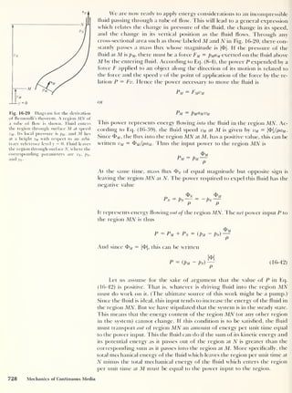
![Fig. 16-18 A tube of flow. Typical
streamlines within the tube are shown
as clashed lines. All fluid passing through
the tube must first penetrate the planar
cross section M and later the planar
cross section N.
But even if we imagine a certain volume of an ideal (and therefore
incompressible) fluid to be flowing through a system of pipes, tanks, and so
forth, the shape of this volume generally will not remain constant. If the
pipe narrows, for instance, a squat, cylindrical volume of fluid will become
long and thin, as the "front” end of the cylinder enters the narrow region
hrst and speeds up first. To deal with this difficulty, we introduce the con-
cept of the tube of flow. We assume that the fluid flows steadily. In this
so-called steady state each microscopic element of fluid follows a stream-
line (see the definition of streamline in Sec. 16-6). You may think of a tube
of flow as a bundle of streamlines, as illustrated in Fig. 16-18. In the ab-
sence of viscosity, all elements of the fluid on any surface normal to the
streamlines flow at the same speed. 1 bus elements of fluid which are simul-
taneously located on the plane surface M will later find themselves simul-
taneously on the plane surface N.
It follows directly from the definition of a streamline that no fluid
enters or leaves the tube of flow through its sides. However, every bit of
fluid which crosses the surface M must later cross the surface N. Since the
flow is steady, the masses of fluid crossing these surfaces per second are the
same.
This is true for steady flow even if the fluid is compressible. To see this, imag-
ine a hypothetical tube of flow in which the fluid density is uniform, except in one
region where it has some greater value, because the pressure there is greater. Even
though this region contains more fluid per unit volume than the rest of the tube of
flow, matter must leave the region at the same rate as it enters or else the local den-
sity will change, in contradiction to what we mean by steady flow.
The rate at which mass crosses a surface is called the flux. More specifi-
cally, the rate of flow of mass is called the mass flux <I>. That is, if in time dt
the mass dm crosses the surface, then the mass flux is defined to be
(16-35)
[See Sec. 12-6 for a different but related use of the concept of flux. In the
three-dimensional situation considered there, we used the symbol S to rep-
resent the (energy) flux —that is, the (energy) flow per unit time —across a
unit area. Here we use the symbol <f> to represent the total (mass) flux —that
is, the (mass) flow per unit time —across a surface of arbitrary area a. The
relation between the two quantities is S = df/m]
It is useful to reexpress Eq. (16-35) in terms of the density p, the mass
per unit volume. From Eq. (16-16) we have
m — pV
where the mass rn of fluid occupies a volume V. Since the density p is a
constant for an incompressible fluid, we can substitute this expression into
Eq. (16-35), writing dm = p dV to obtain
dV
cfi = p— (16-36)
It is often convenient to consider flux $ as a signed scalar, with flux
into a closed region having a positive value and flux outward having a negative
value. For the region enclosed by M and N in Fig. 16-18, you can see that
= -&M (16-37)
726 Mechanics of Continuous Media](https://image.slidesharecdn.com/robertm-220626164724-d75ac43b/85/Robert-M-Eisberg-Lawrence-S-Lerner-Physics_-Foundations-and-Appli-pdf-50-320.jpg?cb=1675858377)
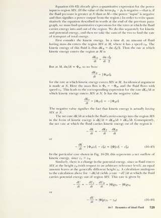
![Since the flux through the walls of the tube is zero, Eq. (16-37) can be
written in the more general form
Fig. 16-19 A tube of flow shown in
profile. All fluid located on the surface
M at a certain instant lies at a time dt
later on another surface located a dis-
tance ds downstream. The local speed of
the fluid is vM = ds/dt. A similar state-
ment can be made about fluid which at
a certain instant lies on the surface N.
But if the area aN of surface N is not the
same as the area aM of surface M, then
vN / vM .
v o = o (16-38)
entire
surface
where “entire surface" includes M, N, and the boundary of the tube of flow
between them. Either Eq. (16-37) or (16-38) is called the continuity equa-
tion. The continuity equation says simply that the net amount of fluid en-
tering the tube of flow is zero, provided that fluid is neither created nor
destroyed within the tube. It is true of any closed region in a steadily flow-
ing fluid, provided that there are no sources, or sinks, of fluid within the
region —that is, places where fluid “appears” or “disappears.” The conti-
nuity equation is of fundamental importance in the theory of fluids, where
it is quite clear what is flowing. As you will see in Chap. 20, it is equally im-
portant in the theory of electricity, where what is “flowing” is not fluid but
the much more abstract entity called electric field.
Associated with the fluid is a velocity. Consider an imaginary surface,
moving with the fluid, which passes through the stationary surface M at a
certain moment. At a time dt later, the moving surface will have passed
downstream an infinitesimal distance ds, as shown in Fig. 16-19. Since ds is
infinitesimal, the cross-sectional area of the tube of flow will not be appre-
ciably different from aM,
its value at M. The volume dV of the space con-
tained between M and the moving surface contains all the fluid which has
passed through the surface M in the time dt, and no other fluid has entered
this space. The volume of fluid passing M in time dt is thus
dV = aM ds
Equation (16-36) can therefore be written in the form
ds
4>m = pau
it
Since vM — ds/dt is the speed of fluid flow at M, this can be written
<$>m = paMvM (16-39)
The same argument can be applied at any other location along the tube of
flow, so that in general at any location the flux has magnitude
|<f>| = pa(s)v{s) (16-40)
where a and v are functions of the distance s along the curved path fol-
lowed by the fluid. [Compare this equation with the analogous equation,
Eq. (12-62) for energy flux, which in our present notation would be written
|<f>|/a = pv.]
Now take the case of an incompressible fluid, where p is constant.
Combining Eq. (16-40) with Eq. (16-37), the continuity equation for any
two surfaces M and N, immediately yields
Vm _ <Zn
vN aM
(16-41)
That is, for an incompressible fluid the flow speed is inversely proportional
to the cross-sectional area of the tube of flow.
16-7 Dynamics of Ideal Fluid 727](https://image.slidesharecdn.com/robertm-220626164724-d75ac43b/85/Robert-M-Eisberg-Lawrence-S-Lerner-Physics_-Foundations-and-Appli-pdf-51-320.jpg?cb=1675858377)
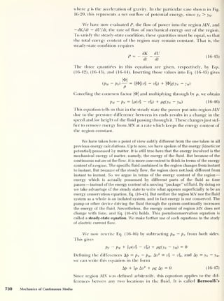
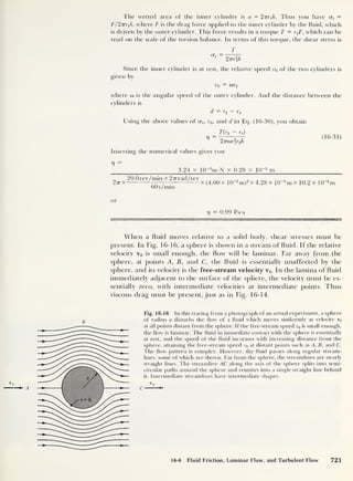
![Fig. 16-21 Application of Bernoulli’s theorem
to steady flow in a nonlevel pipe of uniform
cross section. The theorem gives the change
in pressure from plt the value at a location
having height ylt to p2 ,
the value at a location
having height y2 . The speed of the fluid does
theorem, after Daniel Bernoulli (1700-1782), a noted mathematician and
physicist from a family of many distinguished Swiss mathematicians, physi-
cists, and other scholars. Bernoulli made significant contributions to the
theory of differential equations and to the theory of fluids.
Bernoulli’s theorem has a number of important, simple, special cases.
If we set v = 0 everywhere (the hydrostatic case), then Aw2 = 0, and
Ap
= - pg Ay (16-48)
This is just Eq. (16-17) written in a slightly different form. Even if the flow
speed is not zero but is the same everywhere (as is the case for a pipe of con-
stant cross section), Eq. (16-48) still holds. This is illustrated in Fig. 16-21.
While such a case differs from the hydrostatic case in that the fluid has
kinetic energy, the kinetic energy does not change as the fluid moves along.
Thus any increase in the gravitational potential energy of the fluid per unit
volume [the third term in Eq. (16-47)] must be accompanied by a numeri-
cally equal decrease in the pressure, just as in the hydrostatic case. T his is
illustrated in Example 16-9.
EXAMPLE 16-9
The tank shown in Fig. 16-22 is kept filled with water to a depth of 8.0 m.
a. Find the speed with which the jet of water emerges from the small pipe
just at the bottom of the tank.
You apply Bernoulli’s theorem to the differences Av2
, A p, and Ay between
the locations t and b in Fig. 16-22. Since the tank is large and the pipe is small, you
can neglect the speed with which water at the top of the tank descends through the
tank to replace the water flowing out via the jet at the bottom. That is, the water has
negligible speed until it is actually in the outlet pipe. In applying Eq. (16-47), you
can therefore write
An2 = vl - 0
so that
The water surface in the tank is at atmospheric pressure. But so is the water jet,
which consists of water that has emerged from the tank and is not subject to the
16-7 Dynamics of Ideal Fluid 731](https://image.slidesharecdn.com/robertm-220626164724-d75ac43b/85/Robert-M-Eisberg-Lawrence-S-Lerner-Physics_-Foundations-and-Appli-pdf-55-320.jpg?cb=1675858377)
![fixed total volume Vp Fig. 16E-37
a. Find p'
A ,
p'
B ,
V'
A ,
and VB in terms of pA , pB ,
VA ,
and
VB .
b. Obtain numerical values for p'
A /pA and for V'
A /VA
for the case pB = 3pA and VB = 2VA .
16-38. Steel spheres, II. Consider one of the sinking
steel spheres described in Exercise 16-25. Assume that the
sphere is small enough that the flow is laminar, even at
terminal speed. Furthermore, assume that as the sphere
accelerates from rest to its terminal speed, the viscous
drag force is given by Stokes’ law, Eq. (16-32), at each in-
stant, with v0 being the instantaneous speed vs of the
sphere.
a. If the sphere is released from rest at time t
= 0,
find its speed vs as a function of time t.
b. Find the distance ds through which the sphere
descends in time t.
c. How long is required for the sphere to reach each
of the following fractions of its terminal speed? (1)
1 - /e = 0.63; (2) 0.90; (3) 0.99.
d. What are the distances that correspond to the
times found in part c?
e. Evaluate numerically the results of parts c and d
for a sphere of radius rs = 50 pan = 5.0 x 10
-5
m. How
many times its own diameter does this sphere descend be-
fore reaching 99 percent of its terminal speed?
16-39. Tiny bubbles. Show that when a small gas
bubble is formed underwater, if buoyancy were the only
important force, the bubble would have an initial upward
acceleration much greater in magnitude than g. The
rapid rise of small bubbles can be observed in a glass of
carbonated beverage. (Hint
:
Refer to Exercise 16-38a,
and assume that the gas is approximately at atmosphere
pressure so that its density is p„ — 1.22 kg/m3
.)
16-40. Deriving the generalform of Stokes’ law by dimen-
sional analysis. Assume that the drag force F acting on a
sphere falling through a fluid depends only on the viscos-
ity r] of the fluid, the radius r of the sphere, and the veloc-
ity v of the sphere. The force must then be given by an
equation of the form F = (constant) 7)
xrvif,
where x, y,
and z are exponents whose values you would like to deter-
mine and the constant is dimensionless. By considering
the known dimensions of the quantity F, and the known
dimensions of the quantities 17, r, and v, show that x = y
=
z = 1 , so that the force is given by an equation of the form
F = (constant) 7yv. Compare this result with Stokes’ law,
Eq. (16-32).
16-41. Poiseuille’s law. In Fig. 16-14, the speed of the
fluid in laminar flow is proportional to the first power of
the distance from the stationary plate. This is also approx-
imately true in the rotating-cylinder viscometer of Fig.
16-15. However, when fluid flows through a cylindrical
pipe of radius R and length Lin a direction parallel to the
pipe axis, the result is otherwise because of the different
geometry. Imagine the fluid in the pipe to be subdivided
into cylindrical shells of infinitesimal thickness. These
shells correspond to the laminae of Fig. 16-14. The outer-
most shell, in contact with the pipe itself, moves with neg-
ligible speed. Shells of successively smaller radii move with
successively greater speeds, being driven by the pressure
difference between the ends of the pipe.
The shear stress at any location within the fluid is still
given by Eq. (16-29), expressed in the differential form
dv
This stress has the same value at any point on the surface
of a cylinder of radius r (where r < R) and surface area
27rrL. The retarding force exerted on that cylinder by the
fluid outside it is thus of magnitude F = crs 2TTrL. Since in
the steady state none of the fluid within the cylinder of
radius r is accelerating, the net force exerted on the cylin-
der must be zero. This is possible only if the retarding
force is equal and opposite to the driving force due to the
pressure difference Ap between the ends of the cylinder.
That driving force is given by the product Apirr2
,
where
rrr
2
is the area of either end of the cylinder.
a. Show that the above argument leads to the equation
dv = — AP
2t)L
r dr
b. Integrate this equation to obtain the relation
between v and r for laminar flow in a cylindrical pipe.
{Hint: Set the limits of integration at the inner surface of
the pipe, where the fluid speed is zero, and at the surface
of an arbitrary cylinder of radius r, where the fluid speed
is v.)
c. Show that if the density of the fluid is p, the fluid
flux through the pipe is given by
77 p ApR*
$ =
8 r] L
fhis relation is known as Poiseuille’s law.
16-42. Mariotte’s bottle. If water runs out of an opening
near the bottom of a full container with an open top,
the exit speed of the water will decrease as the level of the
water drops. If a steady rate of flow is desired, the arrange-
ment shown in Figure 16E-42, called Mariotte’s bottle, can
be used. The bottle is initially completely full of water.
When the water level has fallen so that it lies a (decreasing)
distance h + hi above B within the bottle, and a (fixed)
distance h above B within the tube (actually at the bottom
of the tube):
a. What is the pressure at A?
Exercises 741](https://image.slidesharecdn.com/robertm-220626164724-d75ac43b/85/Robert-M-Eisberg-Lawrence-S-Lerner-Physics_-Foundations-and-Appli-pdf-65-320.jpg?cb=1675858377)
![b. Apply Bernoulli’s theorem to obtain the speed of
flow at B.
c. What is the pressure of the air trapped in the
bottle above the water surface?
d. What happens to this pressure as water flows out
at Bit What causes this pressure change?
16-43. Letting it out. The opening near the bottom of
the vessel in Fig. 16E-43 has an area a. A disk is held
against the opening to keep the liquid, of density p, from
running out.
Fig. 16E-43
a. With what force does the liquid press on the disk?
b. The disk is moved away from the opening a short
distance. The liquid squirts out, striking the disk inelasti-
cally. After striking the disk, the water drops vertically
downward. Show that the force exerted by the water on
the disk is twice the force in part a.
16-44. Undershot water wheel. In Fig. 16E-44, a steady
stream of water of cross-sectional area a and speed v strikes
one of the vanes of an undershot water wheel in an ap-
proximately normal direction.
a. If the vanes are moving with speed V, what is the
magnitude of the force exerted by the water stream on the
vane? Assume that the water drops vertically from the
vane after impact.
b. What is the power obtained from the wheel?
c. What is the desired relation betwen V and v for
maximum power?
Fig. 16E-44
d. What is the efficiency of the system at maximum
power? [Efficiency is defined to be the ratio of output
power to input power (or input energy per unit time).]
16-45. Leaky can. A water-filled can sits on a table.
The water squirts out of a small hole in the side of the can,
located a distance y below the water surface. The height of
the water in the can is h.
a. At what distance x from the base of the can,
directly below the hole, does the water strike the table top?
Neglect air resistance.
b. Flow far from the bottom of the can must a second
small hole be located if the water coming out of this hole is
to have the same range x?
c. How far from the surface of the water must the
hole be located to give the maximum range?
742 Mechanics of Continuous Media](https://image.slidesharecdn.com/robertm-220626164724-d75ac43b/85/Robert-M-Eisberg-Lawrence-S-Lerner-Physics_-Foundations-and-Appli-pdf-66-320.jpg?cb=1675858377)
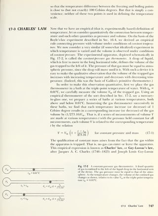
![first to suggest the use of an absolute temperature scale. Kelvin made an enormous
number of important contributions to science and engineering, notably in thermo-
dynamics and electricity.
The use of the Kelvin scale makes possible a simplification of Eq.
(17-1). Using the second of Eqs. (17-2) and noting that i tp = 0.01°C, we
obtain for the volume V at any Kelvin temperature T the relation V =
Vtp[l + (T — 273.15 - 0.01)/273.16], or
T
V = Ttp
— for constant pressure and mass (17-3)
This equation shows that the volume of an ideal gas is directly proportional to its
absolute temperature. In order to stress the fundamental importance of this
point, we rewrite Charles’ law in the general form V/T = Ttp/273.16, or
V
— = constant for constant pressure and mass (17-4)
In Example 17-1, Boyle’s law and Charles’ law are used to describe the
behavior of a quantity of confined gas as its pressure and its temperature
are changed.
EXAMPLE 17-1 ———
^
The cylinder shown in Fig. 17-3 is equipped with a leakproof piston. A pointer at-
tached to the piston rod and a scale provide a means of measuring the cylinder vol-
ume V at any time. The cylinder is also fitted with a pressure gauge, so that the pres-
sure p of the gas trapped inside it can also be measured.
a. The apparatus is immersed in a bath of ice water. Its temperature is thus
7 = 273 K. The position of the piston is adjusted until the cylinder volume is V1 =
1.000 liter (L) (1 L = 1 X 10~3
m3
). The pressure gauge shows that the gas pressure
inside is px = 1.000 atm. With the apparatus still immersed in ice water, the piston
is pulled out until the pressure gauge reads p2 — 0.333 atm.
A gas heater under the bath is then turned on. All the ice melts, and the bath
temperature then slowly rises until the water begins to boil. The system thus comes
to a final temperature T3 = 373 K. During this process, the piston is moved as neces-
sary to keep the pressure reading constant. Thus the final pressure reading is p3 =
p2 = 0.333 atm. What is the final cylinder volume V3 read on the scale?
The process has two parts, shown schematically in Fig. 17-4a. In the first
part, the temperature of the system remains constant, being fixed at the freezing
point of water. Since the piston is leakproof, the mass of the gas in the cylinder re-
Fig. 17-3 Illustration for Example 17-1.
I I I I II I
II I I I II I I I
Y I II I I I I II I r I TTT
V
Volume scale
17-3 Charles' Law 749](https://image.slidesharecdn.com/robertm-220626164724-d75ac43b/85/Robert-M-Eisberg-Lawrence-S-Lerner-Physics_-Foundations-and-Appli-pdf-73-320.jpg?cb=1675858377)
![The denominator of this fraction can be expressed in the form [mass of 1
molecule (in u)] x [1 u (in kg)]. Thus we have
Number of molecules in 1 kmol
_ mass of 1 kmol of molecules (in kg) 1
mass of 1 molecule (in u) 1 u (in kg)
The first fraction on the right side of this equation has the numerical value
1, because of the definition of the quantity 1 kmol. Thus the second frac-
tion, the reciprocal of the atomic mass unit expressed in kilograms, is equal
to the number of molecules in 1 kmol. This number, which is a universal con-
stant, is called Avogadro’s number A. The value of A is determined experi-
mentally to be
A = 6.022 x 10
26
(17-13)
Just as 1 kmol is defined to be the quantity of a substance whose mass in kilo-
grams is numerically equal to the mass of its individual molecules in atomic mass
units, 1 mole (mol) is defined to be the quantity of a substance whose mass in
grams is numerically equal to the mass of its individual molecules in atomic mass
units. One mole contains 10~3
as many molecules as 1 kmol, that is, 6.022 x 10²³
molecules. In chemical practice, where substances are handled experimentally
more often in gram quantities than in kilogram quantities, this is the value usually
quoted for Avogadro’s number. In this book, however, we use the kilomole exclu-
sively, so that the proper value for Avogadro’s number will be that expressed in
Eq. (
17- 13 ).
Since 1 kmol of any substance contains A molecules, n kmol of the
same substance must contain nA molecules. If we call the total number of
molecules present N, it follows that N = nA. Substituting this value of N
into the ideal-gas law, pV = NkT, we have
pV = nAkT
But Avogadro’s number A and Boltzmann’s constant k are both universal
constants. So we may as well lump them together into a single constant. We
define the universal gas constant R to be
R = Ak (17-1 4zz)
The numerical value of R is
R = 6.022 x 10
26
x 1.3807 x 10"23
J/K
or
R = 8.314 x 10
3
J/K (17-14b)
Expressing the ideal-gas law in terms of R, we have
pV = nRT (17-15)
Unlike Boltzmann’s constant, the universal gas constant R can be deter-
mined directly by measuring the pressure p, the volume V, and the temper-
ature T of a macroscopic sample containing a known number n of kilomoles
of some gas under conditions in which its behavior approximates that of an
ideal gas.
The universal gas constant R plays the same role in equations describ-
ing the macroscopic behavior of a gas as Boltzmann’s constant k plays in
equations describing the microscopic behavior of the gas. The relation
17-4 The Equation of State of an Ideal Gas 755](https://image.slidesharecdn.com/robertm-220626164724-d75ac43b/85/Robert-M-Eisberg-Lawrence-S-Lerner-Physics_-Foundations-and-Appli-pdf-79-320.jpg?cb=1675858377)
![b. If the rod is rigidly clamped in a strong holder at 300 K and the rod (but not
the bulk of the holder) is heated to 350 K, find the stress along the axis of the rod
and the magnitude of the force required to hold it. Take Young’s modulus to be
Y = 2.00 x 10“ N/m2
,
and assume that the rod is not stressed beyond its elastic
limit.
If the rod were not clamped, its length would be increased by 1.31 x 10
-3
m.
The uniaxial stress rr in the rod is the same as if the rod had been allowed to expand
freely and had then been squeezed back to its original length. This process would
involve a strain e = A///. And since Young’s modulus is defined to be Y = cr/e, you
have
A/
a = eY = — Y
Using the given numerical values of / and Y and the value of A/ calculated in part a,
you obtain
1.31 X 10'3
m
a = x 2.00 x 10
11
N/m2
2.50 nr
= 1.05 x 10
8
N/m2
The magnitude F of the force is the product of the stress and the cross-sectional
area. The area is 7rr
2
, and the radius r is one-half the rod diameter, 2.00 cm. So you
have
F = 1.05 x 10
8
N/m2
x [> x (1.00 x 10~2
m)2
]
= 3.30 x 10
4
N
This is more than 3 tons.
c. How much mechanical energy is stored in the rod by heating it? That is, how
much mechanical work can it do when it is unclampecl with the temperature at
350 K?
If you assume that the rod is not compressed beyond its elastic limit, it will
obey Hooke’s law when allowed to expand. According to Eq. (7-58), the potential
energy stored in such a system is given by
U =
k(Al)
2
where k is the force constant given by
F
Combining the two equations, you have
U
F A/
I he numerical value is
U = 3.30 x 10 4
N x 1.31 x 10“3
m
= 21.6
In the case of a long, thin rod, the linear expansion is of greatest inter-
est. But the rod expands in girth as well as in length. For a solid of more
general shape, and for all fluids, we are interested primarily in the increase
in volume rather than that of a specific dimension. Like the fractional
linear expansion, the fractional volume expansion —that is, the ratio of the
758 The Phenomenology of Heat](https://image.slidesharecdn.com/robertm-220626164724-d75ac43b/85/Robert-M-Eisberg-Lawrence-S-Lerner-Physics_-Foundations-and-Appli-pdf-82-320.jpg?cb=1675858377)
![one-thousandth that of the kilocalorie, so that 1 cal = 10
-3
kcal. How much water
can be raised in temperature from 14.5°C to 15.5°C by 1 cal of heat?
The British thermal unit (Btu], still used in U.S. engineering practice, is the
amount of heat required to raise the temperature of 1 pound of water from 63° Fahr-
enheit to 64° Fahrenheit. In terms of the kilocalorie, its value is 1 Btu — 0.252 kcal.
The heat capacity C(T) of all substances changes abruptly and signifi-
cantly when they undergo melting, boiling, or similar phase changes. Even
in the absence of such changes, the heat capacities of all substances decrease
rapidly with decreasing temperature when the temperature is low enough.
(For most substances, “low enough” means at temperatures well below
room temperature.) Otherwise, however, the heat capacity for most sub-
stances varies quite slowly with temperature and can therefore be regarded
as constant for many practical purposes. When this is the case, Eq. (17-20)
can be simplified to obtain
[
Tf
AH = C dT — C(Tf - T,)
Jti
Calling AT = T{
— Tu we write this in the compact form
AH = C AT (17-21)
In the particular case where C has the value appropriate to a sample of
matter consisting of 1 kg of water in the temperature range between 14.5°C
and 15.5°C, Eq. (17-21) becomes the definition ofi quantity of heat AH. To see
this, compare Eq. (17-21) applied to this special case with the italicized state-
ment used to define the quantity of heat called a kilocalorie.
It seems plausible (and it is borne out by experimentation) that the
beat capacity of a homogeneous object is directly proportional to its mass m.
We therefore define the specific heat capacity c of a substance as its heat
capacity per unit mass:
c (17-22)
In terms of this quantity (which is the one invariably tabulated) we can
rewrite Eq. (17-21) in the form
AH — cm AT (17-23)
That is, the quantity of heat AH required to change the temperature ofi a homoge-
neous object whose mass is m, and which is made of a substance whose specific heat
capacity is c, by an amount AT is given by the product of the specific heat capacity, the
mass, and the temperature change. If the temperature dependence of c is not
negligible, we can use an equation like Eq. (17-22) to rewrite Eq. (17-20) in
the more general form
f
T
f
AH — m c(T) dT (17-24)
JTf
The units of specific heat capacity are kilocalories per kilogram-kelvin
[kcal/(kg-K)] when SI units are used in defining it phenomenologically,
as we have just clone. Tables often quote the specific heat capacity in units
of calories per grant-degree Celsius [cal/(g-°C]. However, the specific heat
capacity of any substance has the same numerical value in either set of units.
Can yon see why? The numerical value of the quantity c is also often given
in terms of the specific heat ratio, that is, the ratio of the specific heat
17-6 Heat 763](https://image.slidesharecdn.com/robertm-220626164724-d75ac43b/85/Robert-M-Eisberg-Lawrence-S-Lerner-Physics_-Foundations-and-Appli-pdf-87-320.jpg?cb=1675858377)
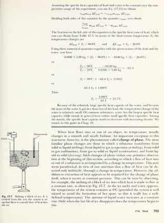
![It has been known since prehistoric times that there is a connection
between friction and heat. Primitive people have made fire by frictional
means for at least 600,000 years. Nails driven into wood are heated sub-
stantially; hammering or drilling on metal can produce enough heat to
make the metal red-hot. And milkmaids have known for a long time that
freshly churned butter is considerably warmer than the cream from which
it is made. (We will soon see the elegant scientific use to which Joule put this
observation.) The idea which these observations suggest —that heat is a
form of motion —dates at least as far as classical Greek times.
In 1620, the great English philosopher Francis Bacon (1561-1626) inquired
into the nature of heat on the basis of the above observations, taken together with a
large number of others. His explicit purpose was to make the study of heat into a
model science, conforming to the rules of scientific investigation which he had
devised. Although his method was open to question from the modern point of
view, he concluded: “Heat is a motion, expansive, restrained, and acting in its
strife upon the smaller particles of bodies. ... If in any natural body you can ex-
cite a[n] . . . expanding motion, and can so repress this motion and turn it back
upon itself, . . . you will undoubtedly generate heat.”
One way of elaborating Bacon’s point of view is to postulate that an in-
crease of temperature of a body implies its molecules are moving faster.
(This motion is random from molecule to molecule, so that the center of
mass of the body does not move at all.) It is possible to measure the me-
chanical energy AE put into a system by friction. If the system is inside a
calorimeter, we can also find the increase A// in the “heat content” of the
system from the measured temperature increase and the known heat
capacity of the system. For that particular experiment, we can then write
the empirical relation
A// = J AT (17-26)
where J is the proportionality constant determined by the experiment. If A//
is measured in kilocalories and AT in joules, the units ofJ must be kilocalo-
ries per joule (kcal/J).
Now suppose that the experiment is carried out with different systems
and with different friction mechanisms. And suppose that (within experi-
mental error) the value of J is always the same. Such a result constitutes
a strong experimental (though indirect) evidence that heat is indeed a
microscopic form of mechanical energy. Moreover, Eq. (17-26) takes on the
character of a universal relation. The quantity J becomes the conversion
factor which relates the arbitrarily defined unit of “heat” —which is now
better called heat energy, or energy in the form of random microscopic
motion —to the fundamental unit of energy, the joule.
I he earliest semiquantitative effort of note in this direction was the
series of experiments performed in the 1780s and 1790s by Rumford.
Benjamin Thompson, Count Rumford (1753-1814), is one of the most
remarkable personages in the history of science. Born of poor parents in colonial
Massachusetts, he died a Count of the Holy Roman Empire. His second wife —he
had abandoned his first when he left the United States —was the widow of the im-
mortal chemist Lavoisier and was herself an accomplished chemist and leader of
Parisian intellectual society. Besides being a physicist, chemist, engineer, nutri-
tionist, and agronomist of the first rank, Rumford was an immensely versatile in-
ventor, a social engineer and reformer, a master Tory spy and a double agent, an
768 The Phenomenology of Heat](https://image.slidesharecdn.com/robertm-220626164724-d75ac43b/85/Robert-M-Eisberg-Lawrence-S-Lerner-Physics_-Foundations-and-Appli-pdf-92-320.jpg?cb=1675858377)
![y
Fig. 18-1 A molecule of mass m mov-
ing with velocity v in a cubical box of
edge length L.
energy K is related to the magnitude p of its momentum by the equation
K = p
2
/2M. [To obtain this relation, write K = Mv2
/
2
and multiply the
right side by M/M to obtain K — (Mv)2
/2M. Then write p = Mil] This
equation can be applied to calculate the kinetic energy K = p
2
/2M trans-
ferred to the wall of mass M when the gas molecule bounces from it, trans-
ferring in the process momentum of magnitude p to the wall. The calcula-
tion tells us that K can be considered to be zero since we can consider M to
be infinite. And since there is no energy transferred to the wall from the
gas molecule, there can be no energy transferred to the gas molecule from
the wall. Our assumption —that a wall of the box is perfectly rigid and in-
finitely massive in comparison to the mass of a gas molecule —leads to the
conclusion that the total mechanical energy of the molecule leaving the wall
after a collision is the same as when the molecule approaches the wall be-
fore the collision.
Figure 18-1 depicts the single-molecule “gas.” For convenience, the
box containing the gas is a cube of edge length L. The molecule has mass m
and at the instant illustrated is moving with velocity v. Every so often, the
molecule bounces from one of the walls in a collision which does not
change its total mechanical energy. We describe these collisions by saying
the molecule collides elastically with the walls. Since no force is exerted on
the molecule except at the walls of the box, we can take the potential energy
associated with the molecule to have the value zero everywhere within the
walls. Then the total energy of the molecule is the same as its kinetic en-
ergy, and we can say that as it bounces elastically from the walls, it main-
tains constant kinetic and total energies. (It should be pointed out that if the
collisions of the molecule with the walls were inelastic, so that it lost energy
in each collision, then in time it would have no energy. The molecule then
would not have the constant motion required by the ideal-gas model. Thus
the assumptions w’hich lead to elastic collisions are consistent with the
ideal-gas model, but ones which lead to inelastic collisions would not be
consistent with the model.)
In terms of its components along unit vectors x, y, z aligned with the
edges of the box in Fig. 18-1, the velocity vector v of the molecule can be
written
v = vx x + Vy y + vz i
Suppose the molecule hits the right-hand wall of the box. We simplify the
calculations, without affecting their final results, by assuming that the force
exerted on the molecule by a wall is always directed normal to the wall and
toward the interior of the box. In this case the force on the molecule acts in
the negative x direction. Hence it changes only the x component of the mol-
ecule’s momentum and therefore only the x component of its velocity, vx.
The force simply reverses the sign of the value of vx. This must be true in
order that the molecule’s speed v = (vx + v + v2
z )
112
be the same after it
hits the wall as it is before, so that its kinetic energy remains constant.
After the molecule strikes the right-hand wall, it moves off to the left.
Which of the five other walls it will strike next we cannot tell in general, but
we know that it must soon strike the left-hand wall. Any intermediate colli-
sions with other walls will not change the x component of its velocity since,
according to our assumption that the forces are normal, these walls cannot
exert forces on the molecule in the x direction. Thus since the distance
between the right- and left-hand walls is L, the time required for the mole-
18-2 Kinetic Theory of the Ideal Gas 779](https://image.slidesharecdn.com/robertm-220626164724-d75ac43b/85/Robert-M-Eisberg-Lawrence-S-Lerner-Physics_-Foundations-and-Appli-pdf-103-320.jpg?cb=1675858377)
![Now N, the number of molecules in the gas, is the product of n, the number of kilo-
moles, and Avogadro’s number A, the number of molecules per kilomole. Thus
N = nA = 1.23 x KT3
x 6.02 x 10
26
Substituting in this value and the value of b, you find
( 3 x 1.0 x 10
-5
m3
y/3
V I677 x 1.23 x 10“3
x 6.02 x 10
26
/
or
r = 9.3 x 10“ n nr
This result provides a fairly accurate determination of the radius of a helium
molecule because such a molecule is very much like an impenetrable sphere, as as-
sumed in Eq. (18-22). Its shape is spherical since the helium molecule consists of a
single helium atom. Furthermore, a molecule of the noble gas helium has a quite
distinct boundary inside which another helium molecule finds it very difficult to
penetrate.
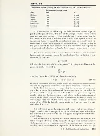
18-4 HEAT CAPACITY One of the striking successes of the kinetic theory of gases is its ability, even
AND EQUIPARTITION * n ' ts simplest form, to predict the heat capacity of monatomic gases. This is
a major subject of this section.
In Sec. 17-6 we introduced the idea of the heat capacity per unit mass
of some material, called the specific heat capacity c, through Eq. (17-23).
Rearranging that equation to obtain an explicit expression for its value, we
have
1 AH
C ~ m ~T
Here m is the mass of the material, AH is the amount of heat added to it,
and AT is its temperature increase. Subsequently we have seen that sup-
plying heat to a gas is a matter of supplying energy to it. Thus we can just as
well specify the specific heat capacity c of a gas in terms of the amount of
energy added to it, AT, in raising its temperature by the amount AT, di-
vided by the mass m of the gas:
1 AE
C ~ m AT
Even if c is a function of temperature, we can still use this relation to evalu-
ate it by taking the limit as AT approaches zero. Doing so, we obtain
1 dE
m dT
(18-23)
When the heat capacity per unit mass c is expressed in this form, the
proper SI units for c are joules per kilogram-kelvin [ J/ (kg- K)].
There is another way of expressing heat capacity which we will find
particularly useful here. It is to define a heat capacity per molecule, called the
molecular heat capacity c'
.
Its value is
1 dE_
nJt
(18-24)
In this expression N is the number of molecules present in the gas, E is its
heat energy content, and T is its temperature.
792 Kinetic Theory and Statistical Mechanics](https://image.slidesharecdn.com/robertm-220626164724-d75ac43b/85/Robert-M-Eisberg-Lawrence-S-Lerner-Physics_-Foundations-and-Appli-pdf-116-320.jpg?cb=1675858377)
![spacing between the atoms is fixed.) The expression for the part of the mol-
ecule’s total energy originating in the energy it absorbs contains five terms:
e = mv + mv% + mv + f/tW] + I2o& (18-27)
The first three terms represent the kinetic energy of motion of the center
of mass, just as for a monatomic molecule. In the last two terms, /, and I2
are the molecule’s moments of inertia for rotation about the axes labeled 1
and 2 in the figure. Axes 1 and 2 are perpendicular to each other, and both
are perpendicular to axis 3 extending along a common diameter of the
atoms in the molecule. (The molecule does not rotate about a diameter of
both atoms because of the same quantum-mechanical property that pre-
vents a monatomic molecule from rotating about a diameter of its single
atom.) The quantities a> 1
and oj2 are the components of the molecule's
angular velocity along axes 1 and 2. Thus the last two terms represent the
kinetic energy of rotation of the molecule about axes perpendicular to the
one that is a diameter of both atoms.
If you review briefly the steps involved in deriving the result
c'v = ik
for the constant-volume molecular heat capacity of an ideal gas or, equally
well, a monatomic gas, you will see that the 3 in the factor | arises because,
on the average, molecules of the gas absorb the same amount of energy in
each of three different ways. Each of these corresponds to one of the three
terms in the energy expression of Eq. (18-26). Next note that the values of
c'
v listed in Table 18-2 for hydrogen, and other gases with diatomic mole-
cules, are all close to the value
C'
v - k
Here the numerator in the fraction multiplying k is 5. And there are five
different ways that the molecule has for absorbing energy, corresponding
to the five terms in Eq. (18-27). This is not a coincidence, but a consequence
of an important theorem, which we now consider.
According to the theorem of equipartition of energy, if molecules are in
thermal equilibrium with their surroundings, then on the average they absorb an
equal amount of energy in each way that they have of absorbing that energy. The
name of the theorem reflects the fact that the energy absorbed by mole-
cules is partitioned (divided) equally, on the average, between the different
ways the molecules have of absorbing energy. [The equipartition theorem
applies only if the terms in the expression for the molecule’s total energy
are each proportional to the square of a velocity component or to the
square of a coordinate —including angular velocity components and angu-
lar coordinates. All the cases we consider satisfy this restriction. See Eqs.
(18-26) and (18-27), and also Eq. (18-28).]
We will give some justification to the equipartition theorem soon. But
first we apply it to a gas ol hydrogen molecules. The theorem requires that
each of the five different ways which molecules of the gas have of absorbing
energy receive, on the average, the same amount of energy, providing the
molecules are in thermal equilibrium with one another. Thus when 5 units
of energy is absorbed by the molecules of the gas in equilibrium, 3 units
goes into increasing the kinetic energy of center-of-mass motion, while 2
units goes into increasing the kinetic energy of rotation. Hence only 3 parts
18-4 Heat Capacity and Equipartition 795](https://image.slidesharecdn.com/robertm-220626164724-d75ac43b/85/Robert-M-Eisberg-Lawrence-S-Lerner-Physics_-Foundations-and-Appli-pdf-119-320.jpg?cb=1675858377)
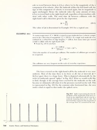
![in 5 of the absorbed energy will be the increase in kinetic energy of
center-of-mass motion that leads to a temperature increase. To put it an-
other way, 5 energy units must be added to the gas to produce the same
temperature increase that would be produced by adding 3 energy units if
the gas were monatomic. As a consequence cl is f times larger than the
value of this quantity for a monatomic gas. Thus the equipartition theorem
predicts the value cl
= f fk = f&, in good agreement with the results
of measurement quoted in Table 18-2.
Figure 18-76 indicates another possible motion of the hydrogen mole-
cule. In this motion the two atoms move with respect to the molecular
center of mass so that the separation between their centers oscillates about
its equilibrium value. The atoms oscillate like two equal balls connected to
opposite ends of a spring. Can molecules in a hydrogen gas absorb energy
by means of an increase in the energy of this motion? Not at T = 300 K, the
temperature at which the value cl — k quoted in Table 18-2 was mea-
sured. We can say this because the factor f has been completely accounted
for by the two motions already discussed.
Bui at much higher temperatures experimental evidence indicates that
absorption of heat energy into vibrational motion does take place. (The ab-
sence of this absorption, except at very high temperatures, is a phenome-
non of quantum mechanics. It is explained in Example 18-6 at the end of
Sec. 18-5.) At T — 3000 K the measured value of cl is quite close to Ik.
This is interpreted to mean that in these circumstances the expression for
the total absorbed energy of a hydrogen molecule contains seven terms.
The expression is
e = mv + mv% + mv + i/jcof + i/2 col + i/uut
2
+ kdr (18-28)
The next-to-last term on the right side of this equation is the kinetic energy
of vibrational motion of the molecule, evaluated by using the reduced-mass
procedure of Sec. 1 1-4. That is, /r is the reduced mass of one of the hy-
drogen atoms, and u2
is the square of its speed of vibration relative to the
other atom of the molecule. In the last term, k is a constant that plays the
same role as the force constant in a harmonic oscillator consisting of a body
attached to one end of a spring. The cpiantity d is the difference between
the center-to-center separation of the two atoms and the equilibrium value
of that separation. Thus the last term is the potential energy stored in the
“spring” (actually, in the electric interaction between the two atoms) in-
volved in the vibrational motion.
Each term in Eq. (18-28) corresponds to a different way that molecules
of hydrogen gas, in thermal equilibrium at a very high temperature, have
of absorbing energy. According to the equipartition theorem, they absorb
the same average amount of energy in each way. Hence 7 units of energy
must be added to the gas to produce the temperature increase that would
result from adding 3 units if the gas were monatomic. And therefore the
molecular heat capacity at constant volume should have the value cl
=
is fk — Ik, as is confirmed by measurement.
The equipartition theorem can be proved from very general arguments. But
the proof is above the level of this book, so we justify it by the following consider-
ations:
1. In cases where a molecule absorbs energy only by increasing the kinetic
energy of its center-of-mass motion [as in Eq. (18-26)], the equipartition of this en-
796 Kinetic Theory and Statistical Mechanics](https://image.slidesharecdn.com/robertm-220626164724-d75ac43b/85/Robert-M-Eisberg-Lawrence-S-Lerner-Physics_-Foundations-and-Appli-pdf-120-320.jpg?cb=1675858377)
![ergy among the x, y, and z components of this motion reflects the fact that there
must be symmetry among the x, y, and z directions. This is essentially the same
argument as used in Sec. 18-2 to derive the ideal-gas law from kinetic theory.
2. When the molecule can also absorb energy by increasing the kinetic energy
of rotation about its center of mass [as in Eq. (18-27)], then we can say that a
self-regulation process —much like the one described in Sec. 18-3 to explain
thermal equilibrium —operates to keep the kinetic energy partitioned equally
among the terms associated with the various components of the motion of its
center of mass and of the rotation about its center of mass. For instance, if by
chance the molecule happens to gain rotational energy in excess of the average
value, then when it next collides with the wall of the container (or with another
molecule), it is likely that it will lose some of this energy and gain some energy of
motion of its center of mass. Think of what would happen if a dumbbell spinning
rapidly about its axis were thrown slowly at a rigid wall.
3. Next consider a molecule in which, in addition, vibrational motion is pos-
sible [as in Eq. (18-28)]. The equipartition of absorbed energy between the poten-
tial and kinetic energies associated with the vibration is easy to understand. Just
look at Fig. 8-16, which is a plot of the potential and kinetic energies of a har-
monic oscillator over several cycles of oscillation. As was noted when the figure
was presented, it shows that even for a single harmonic oscillator the potential en-
ergy averaged over any cycle equals the kinetic energy averaged over the same
cycle.
We can obtain two very useful results by noting that the molecular heat
capacity at constant volume is just the rate of change with temperature of
the average energy content of gas molecules. That is,
cV
die)
dT
(18-29)
Then we note that in all the cases discussed the value ofc^ is observed to be
cV (18-30)
where Jf is the number of terms in the expression for the energy e of a mol-
ecule. For each term in the expression for the energy content of the molecules of a
gas, there is a contribution of k to the molecular heat capacity at constant volume of
the gas, k being Boltzmann's constant. This is an important generalization of
Eq. (18-25), c'
v
= |A, which we derived for an ideal monatomic gas using the
kinetic theory in its simplest form.
To obtain the second result, we note also that if we write the average
value of the energy (e) as
<e>
=Y kT (18-31)
then applying Eq. (18-29) produces immediately the observed values of c'
v
in Eq. (18-30). Hence Eq. (18-31) must give a correct description of the
average energy of the molecules (or of atoms if the molecules are mon-
atomic) in a gas.
In fact, it can be shown that Eq. (18-31) applies to atoms, molecules, or
entities of any type that are in a solid, liquid, gas, or any state. In words, this
form of the theorem of equipartition of energy says the following: If an en-
tity is in thermal equilibrium with its surroundings at absolute temperature T, then
for each term in the expressionfor its energy content e there is a contribution ofkT to
the average value (e) of that energy, k being Boltzmann s constan t.
18-4 Heat Capacity and Equipartition 797](https://image.slidesharecdn.com/robertm-220626164724-d75ac43b/85/Robert-M-Eisberg-Lawrence-S-Lerner-Physics_-Foundations-and-Appli-pdf-121-320.jpg?cb=1675858377)
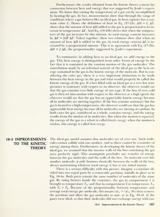
![Thallium vapor
Oven
or
m = 4.65 x 10
-26
kg
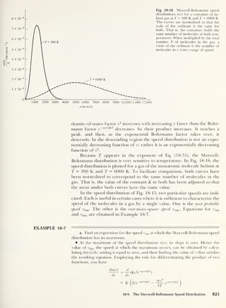
Using this value of m, you evaluate the most probable speed ump thus:
l2kf _ 1
2
x 1.38 x IQ-23
J/K x 300 K
Vmp ~
V m ~ V 4.65 x 10“26
kg
or
urap = 422 m/s
You can then obtain the root-mean-square speed urms most easily by comparing
Eqs. (18-52) and (18-53). They show that
'iv.mp 1.22ump
Hence
urms = 1.22 X 422 m/s
or
urms = 517 m/s
This is about 50 percent larger than the speed of sound in nitrogen gas. Why is urms
comparable to the speed of sound?
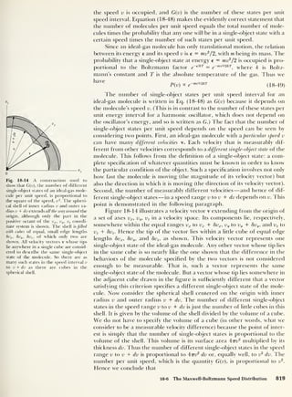
In Sec. 18-5 we proved that the Boltzmann factor has the form e~Bt
for a collec-
tion of objects of any nature. But we proved that /3 = 1/kT only for harmonic os-
cillators not in the quantum domain. There is an enormous amount of physical
theory based on using the factor e~elkT
not just for macroscopic harmonic oscil-
lators but also for microscopic atoms and molecules. For instance, the Maxwell-
Boltzmann speed distribution is obtained by using the Boltzmann factor to calcu-
late occupation probabilities, and the speed distribution is supposed to apply to
molecules. This circumstance makes it possible to test experimentally the applica-
bility of the Boltzmann factor to molecules by comparing the speed distribution
predicted by the Maxwell-Boltzmann theory with the measured speed distribution.
To make accurate measurements of the speed distribution is not easy. The
first real attempt was carried out around 1920 by Stern. Subsequent experiments
by Zartman and Ko from 1930 to 1934, and by others, led to improved results. The
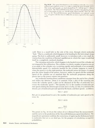
best results to date are those obtained by Miller and Kusch in 1955. The apparatus
is sketched in Fig. 18-17. A vacuum chamber surrounding the entire apparatus is
not shown. A small oven, whose temperature can be controlled very accurately,
contains a supply of thallium metal. The temperature is sufficiently high that a
vapor made up of monatomic molecules of the metal fills the oven. The pressure
(about 10
-6
atm] is low enough that the molecules approximate an ideal gas very
Fig. 18-17 Apparatus used by Miller and
Kusch to measure the speed distribution of an
ideal gas. The entire region is evacuated.
Counter
18-6 The Maxwell-Boltzmann Speed Distribution 823](https://image.slidesharecdn.com/robertm-220626164724-d75ac43b/85/Robert-M-Eisberg-Lawrence-S-Lerner-Physics_-Foundations-and-Appli-pdf-147-320.jpg?cb=1675858377)
![a form of the law of energy conservation, which is known as the first law of
thermodynamics in Chap. 19. But there is a change AS in the entropy of the
total system:
or
AS — ASi + AS2 — dS 1
4- dS
Tu 'ft/
Tu
rr>f dHx
[nr dH2
AS = I -zr1
+
1
T, ,
T1 t2 ,
t2
(18-63)
According to the second law of thermodynamics, the value of AS must sat-
isfy the inequality AS 3= 0. Example 18-10 shows that it does, for a specific
case, by using Eq. (18-63) to evaluate AS.
EXAMPLE 18-10 — " ,ll li rn "i™ 1
A copper can, of negligible heat capacity, contains 1.000 kg of water just above the
freezing point. A similar can contains 1.000 kg of waterjust below the boiling point.
The two cans are brought into thermal contact. Find the change in entropy of the
cold water, of the hot water, and of the total system.
To carry out the integrations required to evaluate the terms in Eq. (18-63), you
must express dHx and dHo in terms of T. In the present case you can do so bv writing
dE = dH in Eq. (18-23) and then solving for dH, to obtain
dH = cm dT
Ehis applies to either the hot water or the cold water if you use c = 4186 J/(kg-K),
the specific heat capacity of water, and m = 1.000 kg. Since the heat capacities of the
two systems are equal, the final temperature will be the average of the initial tem-
peratures:
Tv =
Tu + To, 273 K + 373 K
9
323 K
You thus have
f
T'i dT1 (
T'-r
dT2
AS = ASX + AS2 = cm — + cm—-
J Tu fi Jtu 7 2
Making use of Eq. (7-21) to evaluate the integrals, you find
AS = 4186 J/(kg-K) X 1.000 kg{[(ln 7
’
i )j-j=323 k
— (In T1 )j
'
1=273 k]
+ [(111
7'
2 )r2 =323 K ~ (l n T"2 )7’2 =373 k]}
= 4186 J/K x [In (323 K/273 K) + ln (323 K/373 K)]
= 4186 J/K x (0.168 - 0.144)
or
AS = 703 J/K - 603 J/K
Thus you have ASi = 703 J/K, AS2
= -603 J/K, and AS = 100 J/K.
The entropy of the hot water decreases on cooling, but not as much as the en-
tropy of the cold water increases on warming. So the entropy of the total system in-
creases.
The symmetry of the situation should make it apparent to you that AS will have
a maximum value when Ty = Ty = (Tu + T2i)/2, as assumed. (You can give a nu-
merical proof by evaluating AS for several pairs of values of T^and Ty which differ
by a few degrees from 323 K. How would you prove the statement analytically?)
This means that the entropy S of the total system will have a maximum value when
its two equal parts have reached a common temperature which is the average of
their initial temperatures.
834 Kinetic Theory and Statistical Mechanics](https://image.slidesharecdn.com/robertm-220626164724-d75ac43b/85/Robert-M-Eisberg-Lawrence-S-Lerner-Physics_-Foundations-and-Appli-pdf-158-320.jpg?cb=1675858377)
![Example 18-10 allows us to establish the relation between the concept
of the equilibrium macrostate, introduced in this section, and that of thermal
equilibrium, introduced in Sec. 18-3. Immediately after the two parts of the
total system are put into thermal contact, the total system is not in thermal
equilibrium because the two joined parts are not at the same temperature.
But as the temperature of the initially cooler part increases and that of the
initially warmer part decreases, the two parts approach a common temper-
ature. When both parts have the same temperature, the total system is in
thermal equilibrium. Furthermore, the total system is not in its equilibrium
macrostate immediately after its two parts are joined, but it ends up in the
equilibrium macrostate when they have the same temperature. This is so
because the entropy of the total system is then a maximum. A maximum
entropy means that it is in a macrostate of maximum probability, and this is
the equilibrium macrostate. Hence we can say that when a system is in thermal
equilibrium, the system is in its equilibrium macrostate.
EXERCISES
Group A
18-1. Molecules in a gas mixture. One kilomole of he-
lium gas and one kilomole of argon gas are in a tightly
sealed container whose volume is V = 20 m3
. The gas
mixture is allowed to come to equilibrium at room tem-
perature.
a. What is the average energy of one of the helium
molecules? Of one of the argon molecules?
b. What is the average speed of one of the helium
molecules? Of one of the argon molecules? [One way to
state the average speed is to use the “rms (root-mean-
square) speed.” urms = V
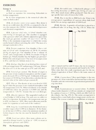
(
v2
) .] Compare your answers with
the speed of sound in air at standard temperature and
pressure, vs
= 330 m/s.
c. Calculate the pressure in the box.
18-2. Ideal gases. Chamber A contains pure helium
gas; chamber if contains pure neon gas. The gas pressures
and temperatures in the two chambers are the same. Each
gas consists of monatomic molecules and can be consid-
ered ideal. The mass of a neon atom is five times the mass
of a helium atom.
a. Compare the number of molecules per unit vol-
ume in the two chambers.
b. Compare the mass per unit volume in the two
chambers.
18-3. Argon gas. A container of volume 8.0 nr
3
con-
tains an ideal gas at a temperature of 300 K and a pressure
of 2.0 X 10⁴
Pa (
— 0.20 atm).
a. What is the total number of gas molecules in the
container?
b. What is the number of molecules per unit volume?
c. What is the total kinetic energy of the gas mole-
cules in the container?
d. Compare the result of part c with the kinetic en-
ergy of a rifle bullet (mass — 3 X 10
-2
kg; speed — 4 x
102
m/s).
e. What is the average kinetic energy per molecule in
the gas?
18-4. Thermal energies. An energy unit that is useful in
the analysis of atomic systems is the electron volt (eV),
which is equal to 1.60210 X 10~19
J.
a. What is the temperature of an ideal gas whose
molecules have an average translational kinetic energy of
1.00 eV?
b. What is the average translational kinetic energy (in
eV) of the molecules in an ideal gas at room temperature
(300 K)?
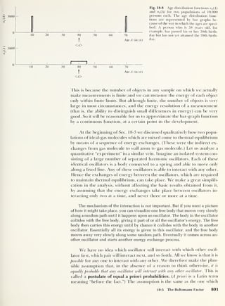
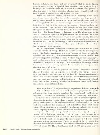
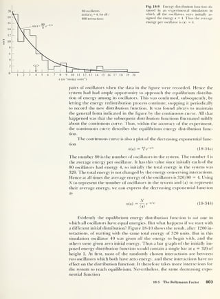
18-5. Avogadro’s law. Avogadro's law states that equal
volumes of ideal gases at the same temperature and pres-
sure have equal numbers of molecules. Show that this
follows from Eq. (18-13) and the equipartition theorem.
18-6. All that glitters is not gold. A collector of precious
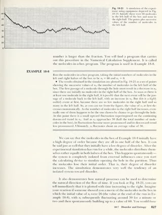
metals compares the amount of heat required to raise by
one Celsius degree the temperature of one gram of gold
and one gram of silver. What does her comparison show?
18-7. Snake eyes. In a throw of three dice, all three
showed one spot. In a second throw, the red die showed a
two, the white die a three, and the blue die a four.
a. Which of the two results was the most probable?
b. Calculate the probability of getting three ones on a
single throw of the dice.
c. Calculate the probability of getting a two, a three,
and a four on a throw, regardless of the color of the dice.
18-8. Not likely.
a. There are n molecules in a container. What is the
probability that, on examination, all the molecules will be
found in the left half of the container?
b. One kilomole of an ideal gas at 0°C and 1 atm pres-
sure contains Avogadro’s number of molecules in 22.4 m3
.
How many molecules are there in one cubic centimeter?
c. Calculate the numerical value of the probability in
part a as a power of 10 if the container has a volume of
one cubic centimeter.
Exercises 835](https://image.slidesharecdn.com/robertm-220626164724-d75ac43b/85/Robert-M-Eisberg-Lawrence-S-Lerner-Physics_-Foundations-and-Appli-pdf-159-320.jpg?cb=1675858377)
![18-9. Molecular energies and speeds in the terrestrial
atmosphere. The hottest naturally occurring air tempera-
ture at the earth's surface is approximately 330 K; the cold-
est air temperature is about 185 K.
a. Express the average kinetic energy per molecule at
185 K as a fraction of the average kinetic energy per mole-
cule at 330 K.
b. Find the corresponding ratio of rms molecular
speeds.
18-10. Entropy change of melting ice. Exactly 1 kg of ice
at its melting point is changed to water without increasing
its temperature. How much has its entropy increased?
18-11. Velocity selector for molecules. In the apparatus
illustrated in Fig. 18-17, the length / of the rotating drum
is 20.0 cm and the angular displacement c
f>
between the
entrance and exit of a molecule from the groove is 5.0°.
See Fig. 18E-11. Calculate the angular speed of the
drum which will select molecules with speeds of 300 m/s.
How many rotations per minute is this?
Group B
18-12. Ideal gas mixtures. In accordance with the law
of partial pressures, in a mixture of ideal gases at temper-
ature T, the total pressure is p = 2j (n/AT) = (tjnj)kT =
n'kT. Here nj is the number per unit volume of gas mole-
cules of type j, and n' is the overall number per unit vol-
ume. Let p'j represent the mass per unit volume of gas
molecules of typej, and let mj represent the mass of each
type j molecule. The “molecular weight" p of type j
molecules is given by pj = Amj, where A is Avogadro’s
number.
a. Show that nj = Ap'j /pj = pj /
b. The average molecular weight (p) and the average
mass per molecule ( m
)
of a gas mixture are defined by
( m) = (p) I
A
= p' /n' ,
where p' is the total mass density:
p' = Ijp'j . Show that (m) = fan] mj) /fen] ).
c. Show that the total pressure p of a mixture of ideal
gases is given by p = p'kT/(m).
d. The average molecular weight (p) of the terres-
trial atmosphere is 28.97 kg/kmol. Find the total mass of
the air in a gymnasium where the temperature T = 295 K
and the pressure p = 1.00 atm. The gymnasium has
dimensions 40 m x 30 m x 10 m. Compare the total
mass you obtain to the mass of an African bull elephant
(6000 kg).
18-13. Helium chamber and mean free path. A chamber
contains (monatomic) helium gas at a pressure of 1.00 atm
and a temperature of 273 K.
a. What is the number per unit volume n of helium
atoms in the chamber?
b. The average separation d between any atom and
its nearest neighbor is given by the approximate equation
d — (
n')~
113
. Evaluate d for the helium gas.
The average distance A that an atom can travel
between successive collisions with other atoms is called the
mean free path. The mean free path is given by the
approximate equation A — 1 /n'cr, where cr is called the
collision cross section. The collision cross section does not
depend on the gas density.
c. For helium atoms at ordinary temperatures, the
cross section a is approximately 1 X 10
-20
m2
. Evaluate
the mean free path for the sample of helium gas described
above
.
d. Suppose the helium chamber is 1 .0 nr in diameter.
At the given temperature of 273 K. how much would the
pressure have to be reduced in order for the mean free
path to be equal to the chamber diameter?
18-14. Energy transfer by moving piston. Consider an
ideal gas confined to a cylinder, one end of which is closed
by an extremely massive smooth piston of aread. The x
axis is perpendicular to the face of the piston, which
moves with velocity wx, compressing the gas. Assume that
the piston’s speed u is much less than the average speed of
a gas molecule.
a. A molecule of mass m impinges on the piston with
velocity v = — |ux |
x + vyy + vzz. What is its velocity after it
strikes the piston? Hint: This question can be answered
fairly easily by examining the collision in a reference
frame where the piston is at rest, considering it to be
elastic.
b. What is the change in kinetic energy of the mole-
cule as a result of its collision with the piston?
c. How much work did the piston do on the mole-
cule?
d. How much work does the piston do on the entire
gas during a time At?
e. Now make the approximation that the speed u of
the piston is very much less than the average molecular
speed and show that the result of part d can be expressed
as W = pA Ax, where Ax = u At is the displacement of the
piston and p is the gas pressure. Why is this a reasonable
result?
18-15. A Clausius gas. Consider a gas of N hard-
sphere molecules which obeys the Clausius equation of
state. The total volume VN of the molecules themselves is
given by VN = N%nr3 = Nv, where r is the radius and v the
volume of each molecule.
a. Show that the Clausius equation of state, Eq.
(18-2 la), can be written as />( 1 — AVN/V) = NkT/V.
b. The Clausius equation is an accurate equation of
state only when VN « V. Show that under this restric-
tion, the following is an accurate expression for the pres-
sure:
NkT
Ua AVn
)
NkT ,
+
4MA
V v J V l V 1
836 Kinetic Theory and Statistical Mechanics](https://image.slidesharecdn.com/robertm-220626164724-d75ac43b/85/Robert-M-Eisberg-Lawrence-S-Lerner-Physics_-Foundations-and-Appli-pdf-160-320.jpg?cb=1675858377)
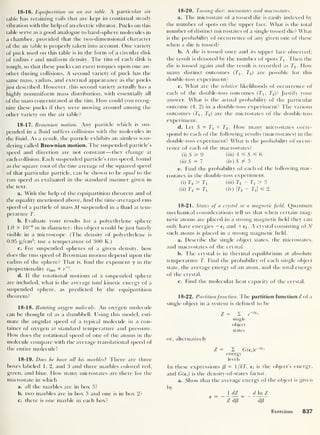
![b. Show that this is also equal to
e = ( kT2
/Z)(dZ/dT
)
18-23. An ideal gas in an imaginary world. Consider an
ideal gas in a two-dimensional world.
a. Modify the arguments leading to Eqs. (18-50) and
(18-51), and find G(v) and n(v) for the ideal gas in two di-
mensions.
b. Find the most probable speed of a molecule in the
two-dimensional gas.
c. Can you generalize these results to an imaginary-
world of D dimensions with D > 3?
18-24. Maxwell-Boltzmann energy distribution. The
number of molecules in an ideal gas having speeds
between v and v + dv is n{v)dv, where n(v) is the
Maxwell-Boltzmann speed distribution function.
a. Using the fact that the kinetic energy of a molecule
is e = imv2
,
find the range of speeds that corresponds to
the range of kinetic energies between e and e + de. Then
express the number of molecules with kinetic energies in
this range as n'(e)de and find n'(e).
b. What is the most probable kinetic energy of a mol-
ecule?
18-25. Molecules in a box. The molecules-in-a-box sim-
ulation is started with 30 molecules in each half of the box.
Show analytically that the probability for the number w(
of
molecules in the left half of the box to monotonically in-
crease to 60 is 1.2 x 10
-21
.
18-26. Entropy and a large heat reservoir. A large heat
reservoir at 100°C in contact with 1 .0 kg of water warms it
to 100°C. Show that there is an increase in the entropy of
the entire system.
18-27. Entropy and two large heat reservoirs. A quantity
of heat// is transferred from a large heat reservoir at tem-
perature Tx to another large heat reservoir at temperature
T2 ,
with Tj > T2 required for spontaneous transfer. The
heat reservoirs have such large capacities that there is no
observable change in their temperatures. Show that the
entropy of the entire system has increased.
Group C
18-28. A mixture of Clausius gases, I. Consider two
monatomic hard-sphere gases a and /3 with atomic radii ra
and rB . A pure sample of gas a obeys the equation
_ NqkT
Pa0 ~ V - Navaa/2
where vaa = in(ra + ra)
3 = 8377T3
. Expressed in words,
vaa is the volume excluded in a collision between two
atoms of type a. A pure sample of gas (3 obeys the com-
pletely analogous equation
NBkT
Pm V - NBvBB/ 2
a. Show that if gases a and (3 are mixed, so that they
must coexist within the same volume V at temperature T,
then the total gas pressure p is given by
= NqkT NB kT
V — Navaq/2 — NBv
q
B/
2
V — NB vBB/
2
— NqVoB /2
where vaB = f
7
r(ra + rB f. (Hint: Carefully account for the
volume excluded by collisions between unlike molecules.)
b. Show that the pressure p given in part a exceeds
the sum of the pressures pa0 and pB0 which each gas would
exert if it were alone in the chamber. Can you suggest a
physical explanation for this result?
c. Show that p > pa0 + pB0 even if we suppose that
rB —» 0. Can you account for this?
d. Show that if the two gases happen to be identical,
then the expression given in part a is in complete agree-
ment with the total pressure that would be obtained by
working directly with the equation for a single sample of
pure a gas (and using a total number of a molecules equal
to the sum Na + NB ). Such agreement is most certainly a
necessary condition for self-consistency; verifying the
agreement can be a source of confidence in a new and
unfamiliar equation, such as that given in part a.
18-29. A mixture of Clausius gases, II. Suppose that two
side-by-side chambers, each with the same volume V, ,
are
separated by a removable partition. One chamber con-
tains a pure Clausius gas of type a (see Exercise 18-28),
while the other chamber contains pure /3-type Clausius
gas. The pressures and temperatures in the two chambers
are equal and are given by pi and Tt ,
respectively. The
partition separating the gases is removed, allowing the
gases to mix and fill the combined volume Vf = 2T,-. The
final temperature Tf equals the initial temperature 7’,-
.
(It
is possible to show that this does not require heat flow into
or from the walls.) Is the final total pressure pf necessarily
equal to the initial common pressure pf If so, why? If not,
why not, and under what circumstances, if any, will pf =
pf
18-30. Dulong-Petit Law. The Dulong-Petit law, Eq.
(18-34), holds true surprisingly well for solids if the tem-
perature is high enough. To predict the behavior of the
heat capacity at lower temperatures, a quantum-mechan-
ical model must be used. One such model, originally used
by Einstein, assumes that all atoms in a solid vibrate at the
same frequency v. The total energy of a solid of N atoms is
then the same as the energy of iN one-dimensional oscil-
lators. The correct quantum-mechanical expression for
the average energy of this collection of oscillators is
(E) = 3Nhv[i + /(e
Bhv - U]
where f3
= 1/AT, and h = 6.63 X 10
-34
J-s.
a. Calculate the heat capacity per atom of the solid,
using this model. Show that it can be written as
c'
where 0 = hv/k.
3R
e
eiT
(e
eiT - l)
2
838 Kinetic Theory and Statistical Mechanics](https://image.slidesharecdn.com/robertm-220626164724-d75ac43b/85/Robert-M-Eisberg-Lawrence-S-Lerner-Physics_-Foundations-and-Appli-pdf-162-320.jpg?cb=1675858377)
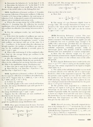
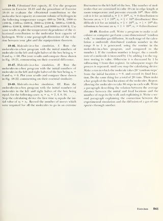
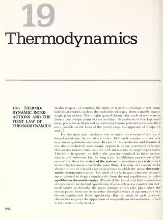
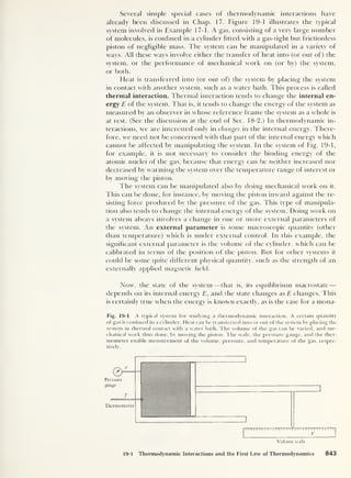
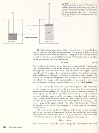
![Fig. 19-6 A heat engine cycle dis-
cussed in Example 19-1. This not very
practical cycle is described by a rectan-
gular curve on a p-V diagram.
N M
0 12 3 4 5
V (in m3
)
3 X 10s
2? 2 X 10
5
a,
c
cs i v in5
EXAMPLE 19-1 11 1 1 11 ——
l lie cycle of a possible (but not very practical) heat engine is shown in Fig. 19-6. A
cylinder having initial volume 3.00 m3
contains 0.100 kmol of helium gas at a pres-
sure of 2.00 X 10
5
Pa (about 2 atm). This state is represented by point K in the fig-
ure. The system expands quasistatically and isobarically, doing work on some ex-
ternal load, until its volume is 5.00 m3
at point L. (In order to keep the pressure con-
stant as the volume is increased, the temperature must be increased. Thus heat
must be flowing into the system during this part of the cycle.) The piston is then
locked in position, fixing the volume, and the pressure is reduced quasistatically
and isometrically to 1.00 X 10
5
Pa at point M. (This is done by slowly cooling the
system, perhaps by placing it in a series of successively cooler baths.) The system is
then compressed quasistatically and isobarically by pushing in on the piston. (In
order to keep the pressure constant as the volume is decreased, the temperature
must be reduced still further.) At point N, with the volume returned to its initial
value of 3.00 nr3
,
the piston is again locked to fix the volume, and the pressure is in-
creased quasistatically and isometrically to its original value of 2.00 X 10
5
Pa, thus
completing the cycle. (In this last step, the temperature must again be increased.)
Find the work AW done on the engine in one cycle KLMNK.
The easiest way to proceed is to equate the work — AW done by the engine to the
area of the rectangle KLMN. That is, the negative displayed in integral of Eq.
(19-6(i) has the value
-AW = Ap AT = (2.00 x 10
5
Pa - 1.00 x 10
s
Pa) x (5.00 m3 - 3.00 m3
)
= 2.00 x 1
0
5
J
Therefore
AW = -2.00 x 10⁵
J
Alternatively, you can get the same result by evaluating
fVL r V„ p, rVK
AW = - pdV - p dV - pdV - p dV
JvK JvL
J vM J v„
= -(2.00 x 105
Pa x 2.00 m3
)
- 0 - [1.00 x 10⁵
Pa x (-2.00 m3
)]
- 0
or
AW = -2.00 x 10
5
J
The negative value of AW, the work done on the heat engine by tbe outside world,
means that the heat engine does positive work on the outside world. You will see in
Example 19-2 that the necessary energy is supplied to the engine from the outside
world in the form of heat.
It was James Watt who first recognized the connection between the enclosed
area of the p-V curve and the mechanical work output of a heat engine (which for
Watt meant the steam engine). Following up this idea, Watt invented the s team
19-2 Isometric and Isobaric Processes 849](https://image.slidesharecdn.com/robertm-220626164724-d75ac43b/85/Robert-M-Eisberg-Lawrence-S-Lerner-Physics_-Foundations-and-Appli-pdf-173-320.jpg?cb=1675858377)
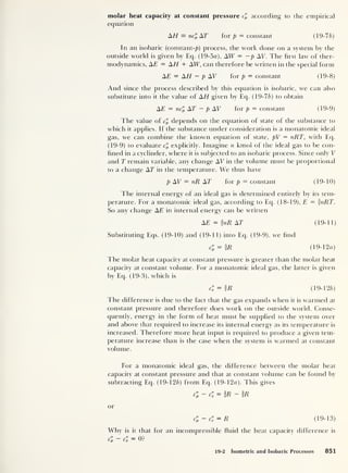
![In Example 19-2 the two molar heat capacities just discussed are used
to calculate the heat input required to drive the heat engine of Example
19-1 through one cycle of operation. Thus the first law of thermodynamics
is used to connect the net work output - AW of the engine with the neces-
sary net heat input AH.
EXAMPLE 19-2
For the heat engine of Example 19-1, find the temperatures of the system in the
states represented by the points K, L, M, and N in the p-V diagram of Fig. 19-6.
Then calculate the heat input, the heat output, and the net heat flow AH into the
system during one cycle.
The working fluid is helium, and since the maximum pressure is only about 2
atm, you can assume that the ideal-gas law is a good approximation, provided the
temperature is always well above the boiling point, 4 K. For any state of the system,
the ideal-gas law pV = nRT gives you
For the state represented by point K you thus have
2.00 x 10
s
Pa x 3.00 m3
r r — — 799 K
A
0.100 kmol x 8.31 x 10³
J/(kmol-K)
At point L the volume is 5.00/3.00 that at K while the pressure is the same. So the
temperature TL is
5.00
Tl = 722 K x = 1203 K
At point M the pressure is 1.00/2.00 that at L, w'hile the volume V is unchanged. So
you have for the temperature TM
1.00
Tm - 1203 K x — = 602 K
And at point N the pressure is 1.00/2.00 that at K, while the volume is unchanged,
so the temperature TN is
1.00
7 " = 722 KX
2700
= 361 K
There is heat flow along all parts of the cycle. As you saw in Example 19-1, heat
must flow into the system along paths NK and KL and out of it along paths LM and
MN. For each of these paths, you can calculate the heat flow by using the relation
AH = nc" AT, provided that you use in each case the value of the molar heat capac-
ity c" which is appropriate to the process taking place and the proper temperature
difference ATif = Tf — T,.
Path NK is isometric and path KL is isobaric, so you have
AHnkl = nc'v A
T
nk + ncl A
T
KL = nR(%ATNK + fATKL )
Inserting the numerical values gives you
AHNKL = 0.100 kmol x 8.31 x 10³
J/(kmobK)
x [f(722 K - 361 K) + §(1203 K - 722 K)]
= 1.45 x 10
6
J
Similarly, path LM is isometric and path MN is isobaric, so you have
AHLMN = nc" ATlm + nc'; A
T
MN = nR®ATLM + §ATMN)
852 Thermodynamics](https://image.slidesharecdn.com/robertm-220626164724-d75ac43b/85/Robert-M-Eisberg-Lawrence-S-Lerner-Physics_-Foundations-and-Appli-pdf-176-320.jpg?cb=1675858377)
![Inserting the numerical values gives you
AHum = 0.100 kmol x 8.31 x 10 3
J/(kmol-K)
x [f(602 K - 1203 K) + f(361 K - 602 K)]
= -1.25 x 10
6
J
Thus there is a net heat flow AH into the system given by
AH = AHnkl + AHlmn = 1.45 x 10
6
J
- 1.25 x 10⁶
J
= 2.0 x 10⁵
J
This positive value indicates that the net heat flow is indeed into the system. The
value of AH is exactly the same as that of — AW, the net mechanical work output per
cycle calculated in Example 19-1. This must be the case in order for the first law of
thermodynamics to be satisfied.
Examples 19-1 ancl 19-2 demonstrate the central principle used in
applying the hrst law of thermodynamics, AE = AH + AW, to the opera-
tion of heat engines. As already noted, neither AH nor AW is a state vari-
able (a variable which can be used to describe the state of a system), and
therefore it is not possible to analyze the behavior of a thermodynamic
system in terms of either taken alone. But their sum AE is a state variable.
Thus its value depends on only the state of the system (represented by a
point on the p-V diagram), not on how it got there. Consequently, the net
change in the internal energy of the system over a closed cycle which begins
and ends at the same point is zero. And since for such a closed cycle AE =
0, the hrst law of thermodynamics becomes 0 = AH + AW, or
AH = -AW
In words, the net heat input to the system over a cycle is equal to the net work
output over the cycle. This general statement was verified for a particular
system in Examples 19-1 and 19-2.
A heat engine is thus a converter of heat energy to mechanical energy. That is,
it converts the disordered microscopic energy of the working fluid (in Ex-
amples 19-1 and 19-2, an ideal gas) into the ordered energy of motion of a
macroscopic object (in the same examples, the piston and whatever ex-
ternal mechanism is linked to it).
An important relation between the molar heat capacity determined
isobarically and the molar heat capacity determined isometrically is their
ratio, called the specific heat ratio y. It is defined to be
[This quantity has nothing to do with the shear strain defined in Eq.
(16-10), for which the same symbol is conventionally used.] For monatomic
ideal gases, the value of y is (5R/2)/(3R/2), or
y = I for monatomic ideal gases
The specific heat ratio y will not have this value for polyatomic gases. But
the only property of ideal gases which is actually significant in evaluating
the molar heat capacity difference c'p — c" is the equation of state, pV —
nRT. So if the behavior of a gas conforms to this equation, the molar heat
capacity difference given by Eq. (19-13), c'p — C = R, will be valid even ifc['
19-2 Isometric and Isobaric Processes 853](https://image.slidesharecdn.com/robertm-220626164724-d75ac43b/85/Robert-M-Eisberg-Lawrence-S-Lerner-Physics_-Foundations-and-Appli-pdf-177-320.jpg?cb=1675858377)
![Fig. 19-9 A p-V plot of a family of isotherms
for 1 kmol of an ideal gas. This family of hy-
perbolas satisfies a set of equations of the form
pV = constant, which is the form assumed by
the ideal-gas law when the temperature is con-
stant. Thus a system whose initial state is repre-
sented by a point on such an isotherm will
always be represented by some point on that
isotherm, as long as the temperature of the
system does not change.
Fig. 19-10 Idealized representation of
a system in which an adiabatic process
can take place. The entire system is sur-
rounded by perfect insulation, so that
no heat can flow into or out of it. (The
heat capacity of the insulation itself is as-
sumed to be negligible.)
flow into or out of it. That is, an adiabatic process is defined to be one in
which A// = 0. [The word is based on the Greek adiabatos, meaning
“impermeable (to heat)."] The first law of thermodynamics, AE = AH +
AW, implies that under such circumstances any work AW done on the
system must result in a change AT in its internal energy. The first law thus
becomes
AE = AW for an adiabatic process (19-18)
What quantity is held constant in an adiabatic process? By definition,
T — constant in an isothermal process, just as p
— constant in an isobaric
process and V = constant in an isometric process. No heat flows into or out
of a system in an adiabatic process. But we cannot express this fact by writ-
ting H = constant, since H is not a state variable. We can use calorimetric
methods to measure the amount of heat A H flowing into or out of a system,
but we cannot specify its “heat H" in a unique manner.
There is. however, a quantity which will serve our purpose —the en-
tropy S. The entropy of a system is well and uniquely defined by Eq.
(18-54),
5 = k In w
where w is the number of microstates of the system contained in the equi-
librium macrostate of interest. Thus S is a state variable. While it is not
usually convenient to measure the entropy of a system in these microscopic
terms, we have already proved that a change in entropy can be expressed
macroscopically in terms of Eq. (18-61),
856 Thermodynamics](https://image.slidesharecdn.com/robertm-220626164724-d75ac43b/85/Robert-M-Eisberg-Lawrence-S-Lerner-Physics_-Foundations-and-Appli-pdf-180-320.jpg?cb=1675858377)
![In an ideal gas, the internal energy depends on only the temperature.
Therefore the relation between dE and dT must be the same, regardless of
the means by which the energy is changed. So even though the change dE is
effected by doing work on the system in a volume c hange instead of by add-
ing heat to the system, so that we have dE = dW instead of dE = dH. we can
still write an equation identical to that obtained by setting dE = dH in the
differential form of Eq. (19-7«), dH = nd'
v dT. That is, the equation
dE = nc'v dT (19-22)
must hold. This is true (for ideal gases only) despite the fact that c", the
molar heat capacity at constant volume, was originally defined (and can be
experimentally measured) in a constant-volume process. Combining Eqs.
(19-21) and (19-22), we obtain
nc'v dT = —pdV (19-23)
In order to apply the equation of state of the ideal gas, pV = nRT, to
this process, we must express it in differential form also. We have
d(pV) = nR dT
But applying the differential form of Eq. (2-15) to evaluate d(pV) gives
d(pV) = pdV + V dp
So the differential form of the icleal-gas law is
p dV + V dp = nR dT (19-24)
Since we want a relation of the form of Eq. (19-20), in which the tem-
perature does not appear, we eliminate dT between Eq. (19-24) and Eq.
(19-23), to obtain
1
pdV + V dp = -nRp dV— (19-25)
ncv
or
Vdp= -
(~ + l) pdV
From Ecp (19-13), we have R = c'p
— c". Thus the quantity in parentheses in
the equation immediately above simplifies to yield
4 + i
Cv
where y is the specific heat ratio defined in Eq. (19-14). Hence Eq. (19-25)
becomes
dp dV
~p
= (19-26)
We now integrate both sides of this differential equation between an arbi-
trary initial state characterized by the pressure and volume pi and Vt
and an
arbitrary final state having pressure and volume pf and Vf . We have
[p, dp _ _ [
v
r dV_
Jp, J
~ ~
7
Jvl
~V
Evaluating the integrals by means of Eq. (7-21), we obtain
(In p)p=Pf
- (hi p)p=p.
= — y[(ln V) v=Vf - (In V) v=v.
]
858 Thermodynamics](https://image.slidesharecdn.com/robertm-220626164724-d75ac43b/85/Robert-M-Eisberg-Lawrence-S-Lerner-Physics_-Foundations-and-Appli-pdf-182-320.jpg?cb=1675858377)
![Since the difference of two logarithms is equal to the logarithm of their
ratio, the equation simplifies to
In — y In
We now use the rule that for any coefficient —a and any argument z, we
have — a In z = In ( z~a
)
= In [( 1
/z)"]. This allows us to rewrite the right side
of the equation immediately above in the form In (V y
/V/). So the equation
becomes
In In
Consequently, pf/pi = Vy
/ Vf . Rearranging terms, we obtain the result
pfV/ = piV
7
for S = constant, ideal gas (19-27a)
1 hat is, the product pVy
remains constant as p and V vary in an adiabatic
process. Since the initial and final states are chosen arbitrarily, we can drop
the subscripts and write
pVy — constant for S = constant, ideal gas (19-276)
That is, when an ideal gas is subjected to an adiabatic process (for which the entropy
S remains constant ), the product of its pressure p and its volume V, ra ised to the power
of the specific heat ratio y, remains constant. You should compare this with
Boyle’s law, pV = constant, which applies to ideal gases under the condi-
tion T — constant.
Example 19-4 applies Eq. (19-27«) to a specific situation.
EXAMPLE 19-4
An insulated cylinder contains helium, for which y = f,
at an initial pressure of 2.00
atm. The piston is allowed to move outward quasistatically until the pressure inside
the cylinder has fallen to 1.00 atm. What is the ratio of the final volume E/to the ini-
tial volume Vi ?
You can write Eq. (19-27a) in the form
Pi
ft.y5/3 = y5/3
Pl ‘
2.00
r
or
2.00
Solving for the ratio of the final to the initial volume, you obtain
Vf
y
= (2.00)
3' 5 = 1.52
Compare this result with that for the isothermal expansion between the same initial
and final pressures, where the ratio is Vf/Vi = 2. Can you explain the fact that the
volume ratios are not the same on the basis of the first law of thermodynamics?
Adiabatic processes can be plotted on a p-V diagram in the same way as
isothermal processes. For an ideal gas, the precise shape of the curve de-
pends on the value of y for the gas involved. Figure 19-11 shows two adia-
batic curves for 1 kmol of a monatomic ideal gas such as helium (for which
y = f) and two for a diatomic ideal gas such as oxygen (for which y = |).
19-3 Isothermal and Adiabatic Processes 859](https://image.slidesharecdn.com/robertm-220626164724-d75ac43b/85/Robert-M-Eisberg-Lawrence-S-Lerner-Physics_-Foundations-and-Appli-pdf-183-320.jpg?cb=1675858377)
![p
(in
Pa)
Fig. 19-1 1 Adiabatic curves shown on a p-V diagram. Isotherms are shown for comparison.
All curves are for 1 kmol of gas. Two adiabatics represent the behavior of a monatomic ideal
gas (7 = J), and two adiabatics represent the behavior of a diatomic ideal gas (7 = f). The
isotherms represent, respectively, the behavior of any ideal gas at T = 273 K and T = 473 K.
Any state of a particular gas is represented by a point on the p-V diagram. That point is the in-
tersection of one adiabatic and one isotherm. The slope of the adiabatic is always steeper than
that of the isotherm at the same point because the exponent 7 is always greater than 1. For a
particular gas, two adiabatics and two isotherms can be used to make up a closed heat engine
cycle. This is exemplified by the curve KLMNK, in which the adiabatics LM and NK are appro-
priate tor a monatomic ideal gas.
Two isotherms are also shown for comparison. Because y is always greater
than 1, an adiabatic curve, usually called simply an adiabatic, is always
steeper than the isotherm passing through the same point.
Since the equation of state links the quantities p, V, and T, the ideal-gas
adiabatic law of Eqs. ( 19-27a) and (19-276) can be rewritten in terms of any
pair of these variables. One way to do this is to rewrite Eq. (19-27a) in the
form
pfVf
_ (Yiy-1
PiVi Vf )
Now apply the ideal-gas law in the form
to obtain
or
PfVf _ ]j
PiVi
~ Tj
Tf vr1
TfV/-1
= TiVT1
(19-28o)
860 Thermodynamics](https://image.slidesharecdn.com/robertm-220626164724-d75ac43b/85/Robert-M-Eisberg-Lawrence-S-Lerner-Physics_-Foundations-and-Appli-pdf-184-320.jpg?cb=1675858377)
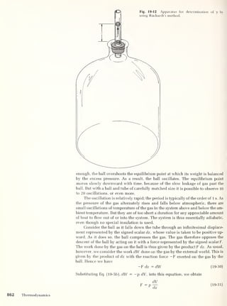
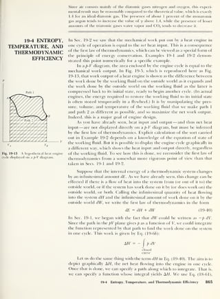
![T
Path 1
Fig. 19-14 A hypothetical heat engine
cycle displayed on a T-S diagram. The
net heat input per cycle to the engine,
A//, is represented by the area enclosed
by the closed curve comprising path 1
from A to B and path 2 from B to A.
Compare with the p-V diagram of Fig.
19-13, in which the area enclosed by the
curve represents the net work output
per cycle from the engine, —AW.
which relates dH to the state variables temperature T and entropy S:
dH
dS=— (19-41)
The equation can be rewritten
dH = T dS (19-42)
By using this relation and the relation dW = —p dV, the hrst law of thermo-
dynamics, dE = dH + dW,
assumes the form
dE — T dS — p dV (19-43)
What has thus been achieved is to write the change dE in the internal en-
ergy of the system entirely in terms of state variables. This was not done in
Sec. 19-2, and we had to calculate the heat flow AH indirectly. But now we
can depict the heat engine cycle in a T-S diagram analogous to the p-V dia-
gram already used.
Figure 19-14 shows a T-S diagram, on which a hypothetical heat
engine cycle is shown. The system passes from state A, whose entropy is SA ,
to state B, whose entropy is SB . along path 1 . It then returns to state A along
path 2. The heat flow AH1
into the system as it passes along path I is found
by integrating Eq. (19-42) to obtain
AH,= [* dH = P" TdS (19-44a)
J A J SA
path 1 path 1
The magnitude of AHl is given by the diagonally hatched area in Fig.
19-14. The heat flow A H2 into the system as it passes along path 2 is
found similarly and is
AH2 = f
A
dH = [
'
TdS (19-44/?)
Jb Js„
path 2 path 2
The magnitude of AH2 is given by the horizontally hatched area in Fig.
19-14. However, AH2 has a negative value, since T is always positive and the
integration proceeds from a greater to a smaller value of S, so that the
value of dS is always negative. (Physically speaking, the positive value of the
quantity — AH2 represents a heat flow out of the system.) The net heat flow
AH into the system over the entire cycle is therefore represented by the dif-
ference between the two areas, which is the area enclosed by the curve com-
prising paths 1 and 2. Expressed mathematically, it is
AH = J
TdS (19-45)
closed
curve
The system states A andB each have a well-defined entropy. According to Eq.
(18-54),
S = k In [w(E)] (19-46)
the entropy depends on w, the number of microstates belonging to the (macro)
state. And w depends on the internal energy E. Thus states A and B each have a
well-defined internal energy E, whatever the working fluid may be.
In the special case of an ideal gas —and only that special case —we need not
appeal to an argument involving the entropy to establish the fact that every point
on a T-S diagram specifies a state with a well-defined internal energy. For an ideal
gas, this fact follows immediately from the dependence of E on T only. And T is
specified for every point on the T-S plane.
866 Thermodynamics](https://image.slidesharecdn.com/robertm-220626164724-d75ac43b/85/Robert-M-Eisberg-Lawrence-S-Lerner-Physics_-Foundations-and-Appli-pdf-190-320.jpg?cb=1675858377)
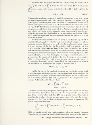
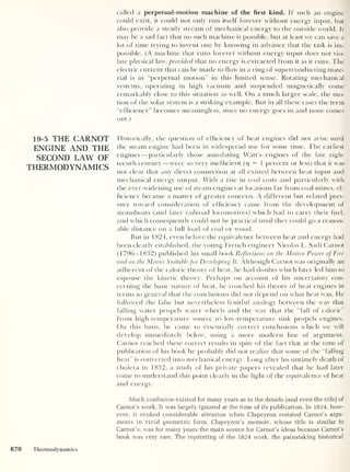
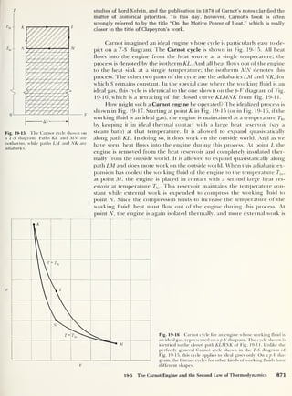
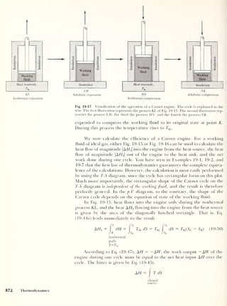
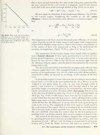
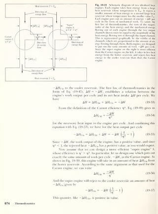
![EXAMPLE 19-8
19-6 HEAT PUMPS,
REFRIGERATORS,
AND ENGINES
HT
—
rTn— uri!,! |
mmm | |( | |
••
—
m
mw—
—
Show that a heat engine which produces no net change in the entropy of the uni-
verse must have efficiency 17 *.
An engine with efficiency rj takes in an amount of heat A//hi ,
whose value is
positive, from the hotter reservoir. The internal energy of the hotter reservoir is
thus changed by the amount - AHhi ,
whose value is negative. At the same time, the
engine rejects an amount of heat - A//l0 , whose value is positive, to the cooler res-
ervoir. The internal energy of the cooler reservoir is thus changed by the amount
— A Hl0 ,
whose value is positive. If the entropy change of the entire system is to be
zero, you must have
as = 0 = ^+
-A//,o
Th Tu
But analogues to Eqs. (19-49) and (19-53) show that A //|0 is given by AH]0 =
AHhl(v — 1 ). Substituting this value into the equation immediately above gives you
0 = AHhi
T!i Tl0 /
Solving for 17 ,
you obtain
T0 7jii To
= —t
—= 17
1 hi 1 hi
which is the Carnot efficiency.
Just as a Carnot engine run in reverse acts as a heat pump, removing heat
from a low-tempeature source and rejecting it to a high-temperature sink,
a properly designed real engine can be made to do the same thing. This is
the basis of the familiar refrigerator as well as the less common, practical
heat pump. The difference between the two is merely a matter of purpose.
The refrigerator is designed to maintain an enclosed space at a tempera-
ture lower than the ambient temperature, so as to store food, to keep peo-
ple comfortable in summer, or for some similar reason. Thus the space
being cooled is itself the heat source, and the outside environment is the
heat sink. Harking back to the general definition of efficiency, that is,
(what you get)/(what you pay for), we characterize a refrigerator by its
refrigerator coefficient of performance Er :
heat removed from source
Er = 7
^ — (19-b8a)
work input to refrigerator
In a heat pump, on the other hand, the aim is to warm an enclosed space by
extracting heat from the cooler outside world and rejecting it into the en-
closure, which thus becomes the heat sink. Here it is more meaningful to
define the heat pump coefficient of performance Ehp
EhP
heat added to sink
work input to heat pump
(19-68b)
These two coefficients of performance are closely related. For a
Carnot heat pump, the coefficent is written Eft
p. It is simply the reciprocal
of the thermodynamic efficiency 77 * given by Eq. (19-52) for the same de-
vice run in the forward direction as an engine. Since the thermodynamic
efficiency is always less than 1 , the coefficient of performance is always
greater than 1. Using Eq. (19-52), we can write
Eft
p = —
Tj*
Thi
878 Thermodynamics Thi Tl0
(19-69a)](https://image.slidesharecdn.com/robertm-220626164724-d75ac43b/85/Robert-M-Eisberg-Lawrence-S-Lerner-Physics_-Foundations-and-Appli-pdf-202-320.jpg?cb=1675858377)
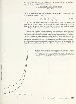
![increasing cost of petroleum products, the relative cost of electricity may fall as
more reliance is placed on nuclear power plants. But whatever the cost of electric-
ity, the cost of using it to drive a heat pump is 1 /Ehp times the cost of direct electric
heating.
If a Carnot refrigerator were available for household use, it might typ-
ically be required to keep food at an absolute temperature T]o = 255 K in
its freezer section, when the household temperature was Thi = 295 K. Its
coefficient of performance would tfius be
255 K
£ ''
295 K - 255 K
That is, each 1
J of input energy transfers 6.4 J
of heat energy out of the
refrigerator compartment. Real household refrigerators have coefficients
of performance about half this large at best. One important reason for this
is a practical one. Il is not economically feasible, from the point of view of
initial capital investment and mechanical reliability, to use a reversible
engine at all. The most common kind of household refrigerator works on
the cycle shown in Fig. 19-22. The compressor (a highly reliable electric
pump) compresses a readily liquefiable gas, usually one of the synthetic
fluorocarbons called Freons. The compression process is more or less adia-
batic. l he heated, compressed liquid passes through a tube to a set of coils
outside the refrigerator. These radiator coils are usually in back, and it is
easy to feel the heat evolved by placing your hand near them. (It is impor-
tant to keep them reasonably clean and to not block the passage of air past
them, so as to minimize Thi .) The compressed liquid, thus cooled to a tem-
perature not too far above room temperature, passes into an expansion
Insulation
Radiator
(outside box)
Fig. 19-22 (a) Schematic diagram of the
operation of the most common form of
household refrigerator. ( b
)
Both p-V and
T-S diagrams of the thermodynamic “cycle”
of the refrigerator. Path 1 represents the
(approximately) adiabatic compression of
the working fluid. (The adiabaticity of this
process is more evident in the T-S plot. Can
you explain the “corner” on the p-V plot
where the gas liquefies?) Along path 2 the
working fluid, which has been heated well
above room temperature in the adiabatic
compression process, cools to approxi-
mately room temperature in the radiator
coils. This process is isobaric, as can be seen
from the p-V plot. The working fluid is then
sprayed through a nozzle located inside the
freezer compartment, vaporizing from liq-
uid back to gas in its rapid expansion. This
Joule-Kelvin expansion is nonquasistatic, and
the working fluid does not pass through a
series of well-defined equilibrium states.
Therefore the process cannot be repre-
sented as a curve on a state diagram such as
a p-V or T-S diagram. When the fluid is
again approximately at equilibrium, its
temperature and pressure have decreased
and its volume and entropy have increased,
as represented by the point at the begin-
ning of path 4. Along path 4, the fluid
warms further in an isobaric process, as it
absorbs heat from its surroundings, and re-
turns to the compressor for another cycle.
880 Thermodynamics](https://image.slidesharecdn.com/robertm-220626164724-d75ac43b/85/Robert-M-Eisberg-Lawrence-S-Lerner-Physics_-Foundations-and-Appli-pdf-204-320.jpg?cb=1675858377)
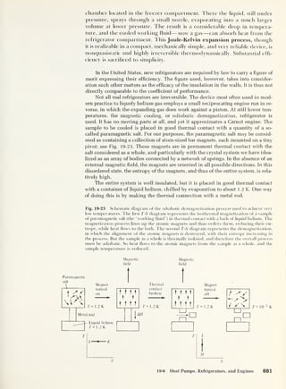
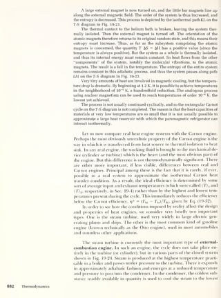
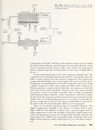
![If we take the condenser temperature Ti0 to be roughly 300 K, the
Carnot efficiency is about 0.63, or 63 percent. The actual efficiency
achieved by the most modern steam plants is about 49 percent. Any sub-
stantial improvement will depend on new technology’s allowing the use of
much higher boiler temperatures.
Nuclear fission steam plants differ thermodynamically from fossil-fuel
plants only in the way that the water is heated. However, the hostile envi-
ronment in which parts of the heating system must operate, subject to in-
tense nuclear radiation, rules out the use of some of the strongest materials
(such as special steels). It also requires that the components be operated at
lower temperatures and pressures than would be possible in the absence of
the radiation. Consequently, nuclear plants are operated at substantially
lower temperatures Thi than fossil-fuel plants. Their overall efficiency is
currently about 30 percent, although improvement is still fairly rapid.
The gasoline engine presents a series of problems which are different
in detail, but still fall into the same general categories. The gasoline engine
is an internal-combustion engine —that is, one in which the heat is pro-
duced by chemical reaction right inside the cylinder. Indeed, all parts of
the cycle take place in the engine proper. As a consequence, the working
fluid cannot recirculate, but is created anew in each engine cycle.
The idealized form of the most important type of gasoline-engine
cycle is called the four-stroke Otto cycle. Its operation is shown schemati-
cally in Fig. 19-25«, and the p-V diagram of the cycle is shown in Fig.
19-256. An air-fuel mixture is drawn into the cylinder during the outward
intake stroke of the piston. The intake valve then closes, and the mixture is
compressed approximately acliabatically during the compression stroke. Near
the point of maximum compression, a spark ignites the mixture, which
burns quite rapidly. Ideally, the combustion is so fast that the piston hardly
moves during its course. Thus the “heat input” to the engine occurs under
isometric conditions. The actual combustion process is far from quasistatic.
It is difficult to measure —or even define —the working fluid temperature
under such conditions. Locally, however, the temperature may reach 6000
K. The effective input temperature is far lower. It is further reduced by the
contact of the hot gas with the cylinder walls, which have a relatively high
heat capacity and are kept relatively cool. In the idealized picture, however,
the hot gas expands more or less acliabatically in the power stroke and then
escapes irreversibly through the exhaust valve, which opens at the end of
the stroke. Finally, the residual working fluid is pushed out of the cylinder
during the exhaust stroke, and a fresh quantity of air-fuel mixture is
drawn in.
It can be shown that the ideal efficiency of tfie Otto cycle is given by the
expression
7]
= 1 - r
J
-y
(19-70)
where r, the compression ratio, is the ratio of the maximum volume of the
cylinder to its minimum volume and y is the specific heat ratio. (This result
applies to the adiabatic compression ratio of Carnot engines as well.) The
practical compression ratio is limited by the cost and availability of fuels
which do not ignite prematurely as they are heated by adiabatic compres-
sion. With lead-free fuels, a practical limit is about r = 9. Since y — 1.4, this
corresponds to an ideal efficiency j)
— 58 percent. In fact, attainable effi-
884 Thermodynamics](https://image.slidesharecdn.com/robertm-220626164724-d75ac43b/85/Robert-M-Eisberg-Lawrence-S-Lerner-Physics_-Foundations-and-Appli-pdf-208-320.jpg?cb=1675858377)
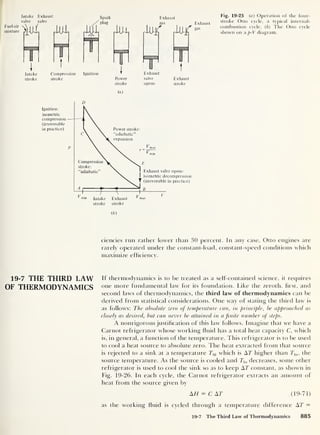
![Fig. 19-26 A hypothetical apparatus
for cooling a heat source to absolute
AH zero. The inability of this idealized
apparatus to carry out its task in a finite
number of cycles exemplifies the third
law of thermodynamics.
Auxiliary
refrigerator
O AH
Heat sink for
T = T = T + AT
1 1
hi Mo Carnot refrigerator
|
AH
Carnot
refrigerator
-i AH
Heat source
T = T]o
to be cooled
to T = 0
Thi
— Co. If we let AT be arbitrarily small, we can use Eq. (19-42), dH =
T dS, and write Eq. (19-71) in tbe form
T dS = C dT
Thus the entropy change of the heat source in one such cycle of the refrig-
erator is
C
dS=jdT (19-72)
If we cool the source from an initial tempeature Tt
to a final temperature
Tf,
we reduce its entropy by an amount
[Tf C
AS = - dT (19-73)
J Ti
1
Ellis is also the amount of entropy which “passes through" the reversible
Carnot refrigerator. That is, the refrigerator increases the entropy of the
heat sink by AS.
Now let us try to make Tf = 0. That is, let us try to cool the heat source
to absolute zero. We then have
AS = f°^dT (19-74)
J 7)
l
The quantity AS on the left side of this equation cannot be infinite.
To see this, note that AS represents the difference S (0) — S(T ; ). The definition
of entropy is given by Eq. (18-54], S = k In [w(E]], where k is Boltzmann’s con-
stant and w(E) is the number of microstates available to the system when its in-
ternal energy is E. At any nonzero temperature T,-, w(E) is a finite number,
886 Thermodynamics](https://image.slidesharecdn.com/robertm-220626164724-d75ac43b/85/Robert-M-Eisberg-Lawrence-S-Lerner-Physics_-Foundations-and-Appli-pdf-210-320.jpg?cb=1675858377)
![19-10. Fill in the blanks. The p-V diagram in Fig.
19E-10 represents a reversible cycle of operations per-
formed by an ideal gas in which MN is an isothermal and
NK an adiabatic. Fill in the chart for this cycle, using + to
indicate an increase in the quantity listed, — to indicate a
decrease, and 0 to indicate no change.
P Fig. 19E-10
Path A AW AE AT AS
KL
LM
MN
NK
19-11. Carnot engine, I. The work output of a Carnot
engine is 1.00 x 10³
J.
Its operating temperatures are
Thi = 400 K and 7j0 = 300 K.
a. How much energy is absorbed by the working sub-
stance during the isothermal expansion?
b. How much energy is rejected to the low-
temperature heat reservoir?
19-12. Carnot engine, II. A Carnot engine removes 16
units of heat from the high-temperature reservoir. Its ef-
ficiency is 1/4.
a. How much heat does it give up to the low-
temperature reservoir? What is the work output?
b. If the temperature of the heat source is 400 K,
what is the temperature of the heat sink?
19-13. Heat pump. A heat pump is to be used to heat a
house to an inside temperature of 20°C. Compare its ideal
coef hcient of performance E*p for the cases when the out-
side temperature is — 10°C (14°F) and when it is + 10°C
(50°F).
19-14. Efficient performance. Show that the relation
between the Carnot efficiency 17
* and the Carnot coeffi-
cient of performance E? is Ef = (1 — r]*)/r}*.
Group B
19-15. Work done by a heat engine. Imagine the cylin-
der and piston arrangement in Fig. 19-1 immersed in a
large tank of water at a temperature of 300 K and con-
taining 0.200 knrol of an ideal gas.
a. What volume must the cylinder have so that the
piston does not move when it is in contact with the open
air at sea level?
b. Now let the same cylinder and piston be immersed
in a large water tank at a temperature of 360 K, and con-
strained from expanding or contracting. What will the
new value be for the pressure of the gas inside the cylin-
der?
c. Finally, let the piston move slowly until the pres-
sure in the cylinder is equal to atmospheric pressure. How
much work has been done by the piston on the sur-
roundings outside of the cylinder?
d. Show all changes in state of the gas in the cylinder
on a p-V diagram.
19-16. Moles following a straight-line path.
a. n kmol of a monatomic ideal gas is taken quasistati-
cally from state A to state C along the straight-line path
shown in Fig. 19E-16. For this process, calculate the work
AW done on the gas, the increase AE of its internal energy,
and the heat AH added to the gas. Express all answers in
terms of pA and VA .
P Fig. 19E-16
b. Repeat part a if the gas is taken quasistatically
from A to C along the path ABC.
c. Explain the similarities and differences between
the results of parts a and b.
19-17. Compressing an ideal gas. n kmol of an ideal gas
is compressed quasistatically at constant temperature
from an initial volume VA to a final volume Vg < VA How
much work was done on the gas to compress it? How
much heat was added to the gas?
19-18. Cycling helium. A sample containing 1.00 kmol
of the nearly ideal gas helium is put through the cycle of
operations shown in Fig. 19E-18.5C is an isothermal, and
pA = 1.00 atm, VA
= 22.4 m3
, pB = 2.00 atm.
a. What are TA , 7 e ,
and F c ?
Exercises 889](https://image.slidesharecdn.com/robertm-220626164724-d75ac43b/85/Robert-M-Eisberg-Lawrence-S-Lerner-Physics_-Foundations-and-Appli-pdf-213-320.jpg?cb=1675858377)
![of n kmol. Show that under adiabatic changes, the gas
mixture obeys an equation of the form pVy = constant.
Obtain an expression for y in terms of ji , y2 ,/i> and /2 •
b. Generalize the result of part a to obtain an expres-
sion for the specific heat ratio y of a mixture of K different
pure gases k. with specific heat ratios yk and fractional
abundances fk ,
for k = 1, 2, . . . ,
K.
19-34. Hang gliders will get a rise out of this. In the
main, the sun’s rays are not absorbed by the transparent
atmosphere but are absorbed by the opaque ground. This
heats the air in contact with the ground, which as a result
becomes less dense than neighboring unheatecl air. The
buoyant force makes the heated air rise. At higher alti-
tudes, the pressure on this rising air decreases so that the
rising air continues to expand. The expansion is essen-
tially adiabatic because of the poor thermal conductivity of
air. Assume that the air is dry so that no condensation
occurs.
a. Show' that the temperature gradient dT/dh, where
T is temperature and h is height, is constant and equal to
Mg (y
— )/y. where M is the mass of one kilomole of air.
b. What is the numerical value of the temperature
gradient? For air, M equals 28.8 kg/kmol.
c. What would be the finite height of such an atmo-
sphere if the ground temperature were 17°C?
19-35. Height of the atmosphere. Exercise 19-34 ex-
plains why, to a hrst approximation, the earth’s atmo-
sphere can be considered to behave adiabatically. Show
that such an atmosphere has a finite height
and calculate hm if the sealevel density p0 were 1.21 kg/m3
corresponding to an average sealevel temperature of 17°C
with p0 equal to one standard atmosphere.
In the actual atmosphere, the rise of air due to its
heating by the warm earth surface continues only to about
1 1 km. The region above this height is called the strato-
sphere.
19-36. Adiabatic pressurizations.
a. A chamber contains n kmol of an ideal gas whose
specific heat ratio is y. The initial volume, temperature,
and pressure are V,- , T, , and p,- , respectively. The gas is now
adiabatically compressed until the pressure is pf . Find the
final volume Vf and the final temperature Tf in terms of
Vi. Ti, pi, pf ,
and y.
b. Obtain numerical values for the ratios Vf /Vt
and
Tf/Ti in the case of pure helium gas (y
= f) or a pres-
sure ratio pf/pi = 2.
c. Obtain numerical values as in part b for pure ni-
trogen gas (y = |).
d. Suppose the chamber described in part a contains
a mixture of n/ 2 kmol of helium and n/2 kmol of ni-
trogen. Use the result of Exercise 19-33 to find the specific
heat ratio for the mixture.
e. Obtain numerical values for Vf /Vi and Tf /Ti if the
helium-nitrogen mixture described in part d is com-
pressed to pf/pi = 2. Compare your results with the corre-
sponding results in parts b and c.
19-37. Entropy of an ideal gas. Consider a sample con-
sisting of n kmol of an ideal gas with specific heat ratio y.
Fet S(T, V) represent its entropy; denote S(T0 , V0 ) by 50 .
a. Show that S(T. V0 )
= S0 + [nR/(y - 1)] In (T/T0 ).
b. Show' that S(T0 , V) = S0 + nR In (V/V0 ).
c. Combine the results of parts a and b to show that
S(T, V) - S0 = nR In + In
Justify your procedure carefully.
d. Which causes a greater entropy increase for a
sample of a monatomic ideal gas, an isothermal doubling
of the volume or an isometric doubling of the absolute
temperature?
19-38. Kelvin’s thermodynamic temperatures. The effi-
ciency of a Carnot cycle does not depend on the nature of
the working substance. (See Sec. 19-5.) That is.
A/7in ~ |A//„ut |
AHm
— f(Thi , 7j0)
or
or
|A/7„U ,|
A/fin
7j0 )
AF/jn
|A//0Ut
1
1 ~ f(Thi > T|0)
F(Thi , ^0)
In 1848, William Thomson, later Lord Kelvin, pro-
posed that F(Thi , 7j0 ) be taken equal to 0hi /0]O . The
quantities 0 are called thermodynamic temperatures and
would be independent of any particular substance. The
thermodynamic temperatures 0 can be shown to be the
same as the temperatures T used in the ideal gas relation
pV = nRT.
a. Referring to Fig. 19-16, for a Carnot cycle using an
ideal gas, calculate A Hm for one kilomole of the gas in
terms of VK , VL ,
and Thi .
b. Calculate |A//0Ut |
in terms of VN , VM , and 7j0 .
c. With the aid ol Eq. (19-28<7), prove that Vl/Vk =
VM/VN .
d. Show that AHjAHouX = Thi /7j0 = 0hi /0io so that
the ideal gas temperatures are the same as Kelvin’s ther-
modynamic temperatures.
19-39. Cooling doiun. A new electric refrigerator has
just been installed in a home, and its temperature is ini-
tially 7 hi ,
the temperature of the surroundings. The
refrigerator’s interior and contents have a total heat
capacity C w'hich does not vary with temperature in the
range 7j0 =£ T =£ Thi . The refrigerator is turned on, and
892 Thermodynamics](https://image.slidesharecdn.com/robertm-220626164724-d75ac43b/85/Robert-M-Eisberg-Lawrence-S-Lerner-Physics_-Foundations-and-Appli-pdf-216-320.jpg?cb=1675858377)
![the interior temperature drops slowly and continuously
until the desired value TUl is reached.
a. Assuming that the internal temperature changes
very little in each cycle of' the refrigerant, show that
the minimum electrical energy Wmin required to complete
the cooling process is given by
wmin = crhi
_ Jjp
Thi , j
b. Evaluate the ratio [Wmin/C(Thi - T]0)] for the case
In )
-
1 lo
Thi = 30°C (303 K) and T,0
= 3°C.
19-40. Pumping heat.
a. Find the coefficient of performance of a reversible
heat pump which is being used to maintain a temperature
of 17°C (290 K) in an enclosure which is surrounded by air
at - 18°C (255 K).
b. Suppose that air from a cave is available for use as
the low-temperature reservoir. If the temperature of that
air is 8°C, what is the coefficient of performance of a
reversible heat pump being used to maintain a 17°C inte-
rior temperature?
c. What percentage savings in work input is obtained
by utilizing a cave-air reservoir? Hint: The rate of heat
loss from the enclosure to the exterior does not depend
upon what is being used as the low-temperature reservoir
in the heat-pump cycle.
19-41. Revived interest in old ideas. Spurred on by the
search for more efficient uses of available fuels, interest
has been revived in the improvement of the Stirling
engine, a hot air engine invented bv the Scottish engineer
Robert Stirling. Operation of this engine is as follows.
First ait' is compressed isothermally at an initial tempera-
ture T0 from an initial pressure and volume p0 and l 0 to
new values pi and Vx . This isothermal compression is then
followed by isometric heating to a new temperature Tj
Next the air is expanded, again isothermally, back to its
initial volume V0 . Finally, tbe gas is cooled isometrically to
the original temperature T0 .
a. Derive an expression for the efficiency of the
Stirling engine in terms of the lower and upper tempera-
tures of the cycle and the volumes for the case of an ideal
monatomic gas as the working fluid.
b. Draw the process on a p-V diagram.
c. On the same diagram indicate the departure from
the ideal case for a gas which follows the van der Waals
equation of state (see Exercise 19-32). How does this de-
parture from the ideal-gas state affect the efficiency of the
engine?
19-42. Entropy change recalculated microscopically. One
kilomole of an ideal gas expands isothermally from vol-
ume V to 2T. Since the temperature is constant, there is no
change in the energy, which is all kinetic. However, the
spatial distribution of the molecules is different. At the
end, half of the molecules are in V on the left of the con-
tainer. Originally all were in this V.
a. Show that the number w of microstates which re-
sult from the possibility of a molecule being in the left or
right half is
o
W
N(N — 1)
• • - 1
) Nl
b. Stirling’s formula for approximating Nl (N-
factorial) when N is large is Nl — NN/e
N. Evaluate w using
this valid approximation and use your result to calculate
the entropy of the gas.
c. How many microstates are there in the macrostate
in which all the molecules are in the left half? Calculate
the change in entropy and compare the result with that
obtained in Exercise 19-23, where the entropy change was
calculated macroscopically.
19-43. Energy, specific heat, and entropy of a two-state
system. A system has only two microstates, with energies
6! = 0 and e2 = e. The results of Chap. 18 can be used to
show that the average energy E(T) for this system is given
by
E(T) = ee~
dkT
/( 1 + e~
dkT
)
a. Find C(T) = dE/dT. Show that C(T) 0 as T 0
and as T —
b. As T 0, the probability that the system is in the
lower state approached unity, so the entropy S —» 0 as
T —> 0. What value should the entropy approach in the
high-temperature limit (AT 55=- e)?
c. Write an expression for S(T) in terms of an inte-
gral over dT' from 0 to T of some quantity.
Exercises 893](https://image.slidesharecdn.com/robertm-220626164724-d75ac43b/85/Robert-M-Eisberg-Lawrence-S-Lerner-Physics_-Foundations-and-Appli-pdf-217-320.jpg?cb=1675858377)
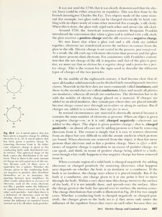
![all either negative, or positive. That is, they spread over the surface of the
body. The interior of the conducting body remains electrically neutral,
fhus for our present purposes everything about a conductor can be ig-
nored except that it has a surface which determines where any charge
placed on it will reside.
The key factor in the behavior of a conductor is that its interior remains elec-
trically neutral, no matter whether it is charged negatively, charged positively, or
uncharged. A formal proof of this is given in Sec. 20-6, but the reason why it
happens can be explained in simple terms here. In its normal state any material is
electrically neutral overall, since there is as much positive charge in the nuclei of
its atoms as there is negative charge in the atomic electrons. When the mate-
rial is a conductor, some of these electrons, called the conduction electrons, are
not constrained to each remain in a particular atom. Rather the conduction elec-
trons are free to move through the conductor. The conduction electrons form
something like a cloud of negative charge. No matter what the state of charge of
the conductor overall, in equilibrium the cloud of conduction electrons must be
distributed through the interior so that any small interior region is electrically
neutral. That is, the total number of electrons in the region equals the total number
of protons. To see this, consider what would happen if in some such region the
cloud of conduction electrons were not dense enough, so that the total number of
electrons was smaller than the total number of protons and the region had a net
positive charge. Then the region would exert attractive forces on the negatively
charged conduction electrons in the cloud adjacent to it. Some of these electrons
would move into the region. The motion would cease only when the region be-
came electrically neutral. The opposite would happen if the region had a net nega-
tive charge. Thus when there is no general motion of conduction electrons in a
conductor, every part of the interior of the conductor must then be electrically
neutral.
The argument above does not apply at the surface of a conductor. This is be-
cause the conditions at the surface of a body are quite different from the condi-
tions in its interior. The different conditions give rise to electric forces acting at
the surface which have different (and more complicated] properties than those
acting in the interior. Hence we cannot argue that the surface of a conductor re-
mains electrically neutral in all circumstances. In fact, it certainly does not do so.
Since in all circumstances the interior of a conductor is electrically neutral when
there is no general motion of charge, any charge that has been given to the con-
ductor must then reside on its surface. Where else can this charge be?
Most of l he qualitative macroscopic properties of the electric force,
and of the electrical behavior of common materials, had been thoroughly
investigated and applied over a wide variety of circumstances by the late
eighteenth century. There was continual improvement in the apparatus
used to produce transfer of electric charge between two objects —that is, to
produce a negative charge on one and an equal positive charge on the
other. (In subsequent chapters we consider modern techniques, such as the
use of a battery.)
As experience with electrical phenomena accumulated, it became evi-
dent that significant further progress depended on determining quantita-
tively the basic properties of l he electric forces that two charged bodies
exert on each other. The two questions which required answers were:
1. How does the electric force vary with the distance between two elec-
trically charged bodies?
2. How does the force vary with the amount of electric charge on each
of the two bodies?
898 The Electric Force and the Electric Field](https://image.slidesharecdn.com/robertm-220626164724-d75ac43b/85/Robert-M-Eisberg-Lawrence-S-Lerner-Physics_-Foundations-and-Appli-pdf-222-320.jpg?cb=1675858377)
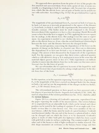
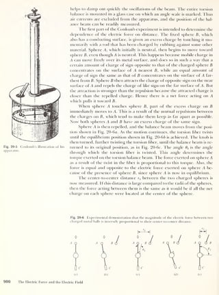
![The justification for this statement involves two things. First, when the
charges added to an isolated metal sphere spread over its surface because of their
mutual repulsions, they end up in a distribution that has the same number of
charges per unit area everywhere. This uniform distribution is a consequence of
the symmetry of a spherical surface. For such a surface any other distribution does
not maximize the spacings between near neighbors. The situation becomes more
complicated if a second metal sphere with the same sign of charge as that of the
first sphere is brought near the first sphere. Now there are repulsions between the
charges in one sphere and those in the other which compete with the repulsions
between the charges on each sphere. The result is that the uniform distribution of
charges on each sphere is disturbed, and there will be some accumulation of
charges in each sphere at the part of the surface farthest from the other sphere. But
if the center-to-center distance between the spheres is large compared to their
radii, the competition will be dominated by the repulsions between the charges on
each sphere. That is, on each sphere the charge will be very nearly uniformly dis-
tributed over the surface.
Second, when charges are distributed uniformly over a spherical surface,
the electric force produced on any external charged object is identical to the force
that would be produced if all these charges were concentrated at the center. This
property is completely analogous to one involving the gravitational force and
a uniform, massive, thin spherical shell. It was justified qualitatively for the
gravitational case in the caption to Fig. 11-5. It is proved quantitatively later
in this chapter.
Sphere B is now brought closer to sphere A, as shown in Fig. 20-6 d.
Sphere A is thus repelled by an increased electric force, and it swings away,
twisting the torsion fiber still further. The adjustable knob is again twisted
sufficiently to return the torsion beam to its original position, as shown in
Fig. 20-6c. The new angle 02 and the new center-to-center distance r2 are
measured. Since r2 < rq, the electric repulsive force exerted on sphere A is
greater than in the former case, and d2 > (fi. That is, it takes a larger twist
of the torsion fiber to balance an increased electric force.
This process can be repeated for different distances and for different
initial charges. (Care must be taken, however, to carry out the measure-
ments quickly, so as to minimize leakage of charge from the two spheres.)
Within the limits of the accuracy of the experiment, the data always
conform to the ride
( 20-
2 )
Since the angle 6 is proportional to the electric force exerted on sphere A
by sphere B, the conclusion is that the strength of this force is inversely pro-
portional to the square of the center-to-center distance between them, all
other factors being held constant. If the separation between the spheres is
large compared to their radii, then the situation is the same as if all the
charge on each sphere were located at the central point, and the center-
to-center distance becomes simply the distance between the two point
charges. Thus Eq. (20-2) is an experimental demonstration of the propor-
tionality between Fkj and 1 /r]k in Eq. (20-1). The accuracy of the experi-
ment is not very high, but later we describe an experiment which confirms
this proportionality to an extremely high degree of accuracy.
I he second part of the Coulomb experiment is intended to determine
whether the electric force Fki has the proportionality to |<7 j|
or to |gfc |,
found
in Eq. (20-1). The situation in Fig. 20-7a is the same as that in Fig. 20-6c.
20-2 Electric Charge and Coulomb’s Law 901](https://image.slidesharecdn.com/robertm-220626164724-d75ac43b/85/Robert-M-Eisberg-Lawrence-S-Lerner-Physics_-Foundations-and-Appli-pdf-225-320.jpg?cb=1675858377)
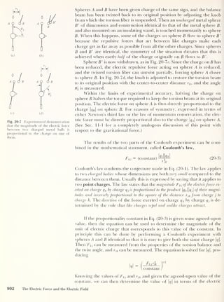

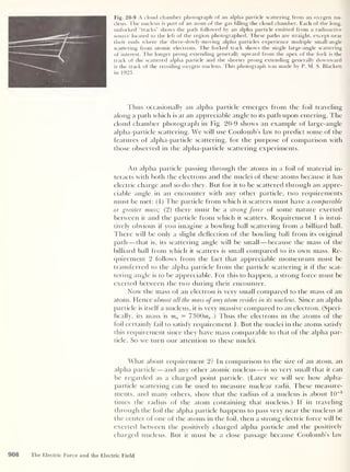
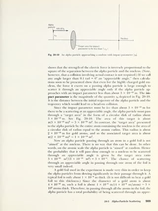
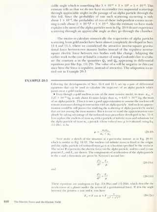
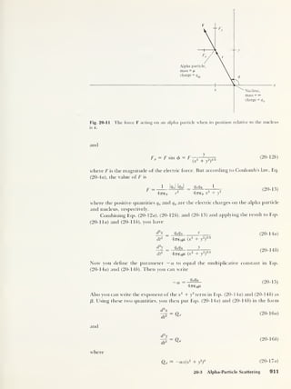
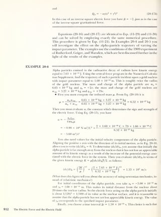
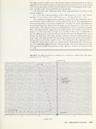
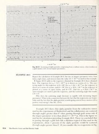
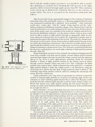
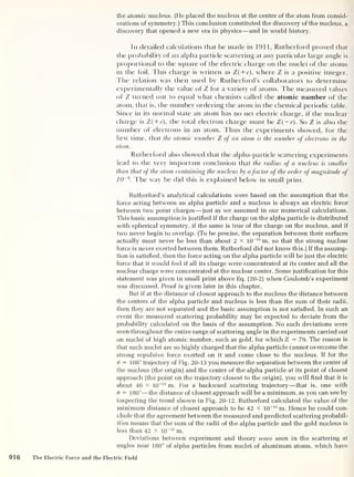
![the low atomic number Z =13. The low charge on the nuclei reduces the repul-
sion they exert on the alpha particles, allowing them to come closer —particularly
for scattering angles near 6 - 180°. Rutherford correctly interpreted the devia-
tions to occur because the alpha particle and nucleus overlap slightly at the point
of closest approach. He then calculated the center-to-center separation at this
point for 6 = 180°, obtaining 7 x 1CT15
m. He suggested that this value represents
an estimate of the sum of the radii of an alpha particle and an aluminum nucleus.
A variety of modern experiments (including the scattering of high-energy alpha
particles obtained from accelerators] show that the radii of the alpha particle and
of the aluminum nucleus are about 2 x 10
-15
m and 3 x 1CT15
m, respectively.
Their sum is in reasonable agreement with Rutherford’s estimate. (The agreement
is very good if 2 x 10
-15
m is added to account for the fact that the strong nuclear
force acts if the surfaces are closer than that amount.)
The value of about 3 x 10 -15
m for the radius of an aluminum nucleus is to be
compared with a value of about 1 x 10~10
m for the radius of an aluminum atom.
(The comparison should not be pushed too far since neither a nucleus nor an atom
has a completely abrupt “edge” like a bowling ball. And some nuclei are noticeably
nonspherical, looking more like a football than a bowling ball. So characterizing a
nucleus or an atom as having a particular radius can be only an approximation.)
The two values lead to Rutherford’s conclusion that the radius of a nucleus is
smaller than that of the atom containing the nucleus by a factor of the order of
magnitude 10
-5
.
20-4 THE ELECTRIC
FIELD AND
ELECTRIC FIELD
LINES
Fig. 20-15 The electric force Ff exerted
on a positive test charge q, by a source
charge q, which is assumed to be posi-
tive. The vector r gives the location of
the test charge relative to the source
charge. The quantity F,/q, is defined to
be the electric field £ of the source
charge at location r.
The electricfield of a charged body is closely related to the electric force that
it exerts on any other charged body. In this section we introduce the elec-
tric held as a device that makes the computation of the electric force more
convenient. Then we show how an electric held can be represented pic-
torially in terms of what are called electricfield lines. In Sec. 20-5 the proper-
ties of electric held lines are used in a simple way to develop a very power-
ful computational and conceptual principle known as Gauss’ law.
In Fig. 20-15 a hxed point charge q is located at a certain position in
space. As a result of the presence of q, any other point charge q t
will experi-
ence a force given by Coulomb’s law. The magnitude and direction of this
force F(
will depend on the position vector r of q t
relative to q. Depending
on the signs of q and q t ,
the direction of Ff is always either the same as or
opposite to the direction of r itself. In principle, we can determine its mag-
nitude Ft
by attaching a small spring scale to q t
and moving it around so as
to measure Ft
as a function of r, the magnitude of its position vector. Also,
Ft depends in direct proportion on the magnitude of q,. If, for example, we
replace q t
with another point charge q'
t = q t /2, then at every position the
force on q', will be just half that on q t
.
If we are mainly interested in exploring the effect of the point charge
q, which we call the source charge, we are not very interested in the value
of the point charge q t ,
which we call the test charge. So let us divide q t
out,
rewriting Coulomb’s law, F< = ( l/47T60 )(qqt
/r2
)r, in a form which gives
the force on the test charge per unit charge of the test charge. We have
Fr
_
1 q
q, 4 7r€ 0 r
2
(20-18)
In this equation F, is the force exerted on the test charge qt
by the source
charge q, r is the distance from the source charge to the test charge, and r is
a unit vector in the direction from the source charge to the test charge. The
force per unit charge acting on a test charge located at some point is known
as the electric field 8 at that point.
20-4 The Electric Field and Electric Field Lines 917](https://image.slidesharecdn.com/robertm-220626164724-d75ac43b/85/Robert-M-Eisberg-Lawrence-S-Lerner-Physics_-Foundations-and-Appli-pdf-241-320.jpg?cb=1675858377)
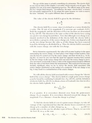
![(a)
/>•
Q
(b)
P
(c)
Fig. 20-16 (a) A charge distribution and
a charge q at point P. ( b )
To find the
force F exerted by the charge distribu-
tion on the charge q, we first find the
electric field £ of the charge distribution
at P. In this step Eq. (20-25) is used, and
there is no reference to charge q. (c)
Then we find F from £ and q. In this
step Eq. (20-26) is used, and there is no
reference to the charge distribution.
Here ¥tj is the force exerted on q t
by the presence of the source charge qj.
Evaluating the terms such as Ftj by means of Coulomb’s law, we have
F, =
47760
Ml f + Ml r i
„2 r lt ^ y 2
r 2f ^
' It '2 1
+ + + q n q t
1
nt
nt
( 20-
22 )
where rjt is the vector from q}
to q t
. Dividing by the common factor q t
gives
us an expression for 8, the electric held of the set of point-source charges:
s-S-
qt 4776n
q i -
r 2
T It
r +
*1/1 o r 2 t
'
rit
+ rjt +
rit
+ q n
nt
nt
(20-23)
This can be written in terms of the electric fields 8j of the individual source
charges qj. To do so, we use Eq. (20-20) and obtain
8 — Si + 8 2 + Sj + + 2, (20-24)
Thus electric fields combine vectorially, just as electric forces combine ac-
cording to the vector addition of Eq. (20-21). In summation notation, Eq.
(20-23) assumes the form
8 = 1
V .
t— 2, 72
4776 0 “ rjt
(20-25)
Equation (20-25) allows us to calculate the electric held 8 of a set of
point-source charges at all positions in space.
Then the electric held at any position can be used to calculate the elec-
tric force exerted on a charge located at that position. This force F is the
force per unit charge acting on a charge at that position, 8, multiplied by
the amount of its charge, q. That is,
F = qS (20-26)
[This is just Eq. (20-19) with the subscript t dropped because the charge q
on which the force is exerted is not a test charge.]
Thus the force exerted by a distribution of charges on some other
charge is calculated in two steps. First, Eq. (20-25) is used to evaluate the
electric held at the location of the other charge. Second, Eq. (20-26) is used
to evaluate the electric force on that charge resulting from the electric held
at its location. The computational convenience of this two-step procedure is
that once 8 has been calculated from Eq. (20-25) for a certain set of
charges, it never has to be calculated again. When 8 is known, Eq. (20-26)
can be used to calculate immediately the force F acting on any other charge
q —no matter what its sign or magnitude. The procedure is indicated sche-
matically in Fig. 20-16.
If only a single point charge is the source of the electric field that acts on an-
other point charge, there does not seem to be much practical advantage in using
the two-step procedure instead of a direct application of Coulomb’s law. This may
be true for the cases presently considered, where at least one of the charges always
is at rest with respect to the observer. But in more general cases involving a pair of
point charges, the two-step procedure made possible by introducing the electric
field (and also the magnetic field present in such cases) can be a necessity —not
just a convenience.
Coulomb’s law describes the electric forces that two separated point charges
exert on each other. If you reread the material at the end of Sec. 4-5, you will be
reminded that such “action at a distance” forces fail to satisfy Newton’s law of ac-
20-4 The Electric Field and Electric Field Lines 919](https://image.slidesharecdn.com/robertm-220626164724-d75ac43b/85/Robert-M-Eisberg-Lawrence-S-Lerner-Physics_-Foundations-and-Appli-pdf-243-320.jpg?cb=1675858377)
![a. You use Eq. (20-25), with n = 3, to write
4776(1
<h
2
1
r It
,
?2 -
+ TIT r2 '
r 2t
Then define x and y axes as shown in the figure so that you can express r u ,
the
vector from to the point P where the held is to be evaluated, as r1( =
(0.200 m)(+x), with x being a unit vector in the positive x direction. Similarly, you
express the other two vectors as r2t = (0.200 m)( — x) and r3( = (0.300 m)(— y).
Then you have
8 = 8.99 x 10⁹
N-m2
/C 2
+ 1.00 x 10
-6
C „
- 2.00 x 10~6
C
(+x) + —(-x)
( 0.200 m)
2
(0.200 m)
= 8.99 x 109
x (7.50 x l(r5
x - 3.33 x 1CT5
y) N/C
+ 3.00 x 10
-6
C , „
-|
(
— v)
(0.300 m)2 v y
The magnitude of the electric held is obtained by using the pythagorean theorem:
S = 8.99 x 10
9
x [(7.50 x 1CT5
)
2
+ (3.33 x KT5
)
2
]
1 ' 2
N/C = 7.39 x 10⁵
N/C
The direction of the electric held can be specihed in terms of the angle 8% between
its direction and the positive x axis. Using the dehnition of the tangent of an angle,
you find its value to be
= tan tan 1
/ —3.33 x 1 Q 5
V 7.50 x ur5
j
-23.9°
The direction of 8 is shown in the hsrure.
o
b. If you know 8 at the point P, calculating the force F which is exerted on a
charge q placed at that point is simply a matter of using Eq. (20-26),
F = r/8
For the magnitude of F you have
F = q% = 4.00 x 10-6
C x 7.39 x 105
N/C = 2.96 N
The direction of F is opposite to the direction of 8 , as shown in the figure, since q
has a negative value. Hence the angle 0F between F and the positive x axis is
8 f = 180° - |%| = 180.0° - 23.9° = 156.1°
It often happens in electrical studies that the situation involves a set of
source charges whose distribution can he regarded as continuous. The elec-
tric held of such a distribution can be calculated by using the methods of
integral calculus. Figure 20-18 shows a region of space over which an elec-
tric charge q is distributed. We wish to find the electric held 8 at point P,
p
<7
Fig. 20-18 A continuous distribution of charge. The
total charge q is subdivided in imagination into infinites-
imal parts clq contained in infinitesimal regions, one of
which is shown. Since these regions approximate points.
Coulomb’s law can be applied to calculating the electric
field at the arbitrary point P outside the charge distri-
bution.
20-4 The Electric Field and Electric Field Lines 921](https://image.slidesharecdn.com/robertm-220626164724-d75ac43b/85/Robert-M-Eisberg-Lawrence-S-Lerner-Physics_-Foundations-and-Appli-pdf-245-320.jpg?cb=1675858377)
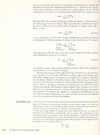
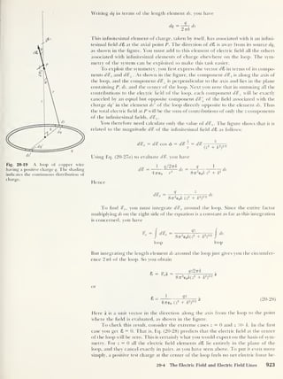
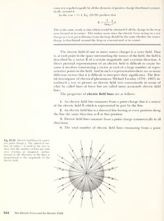
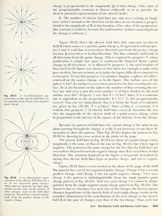
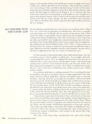
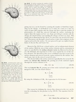
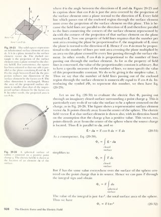
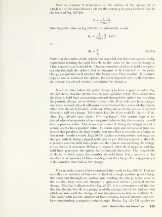
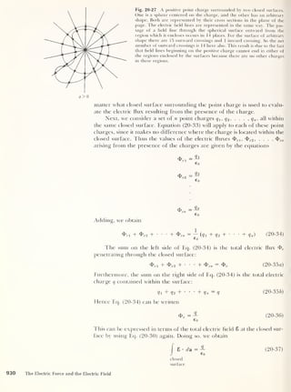
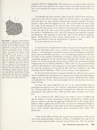
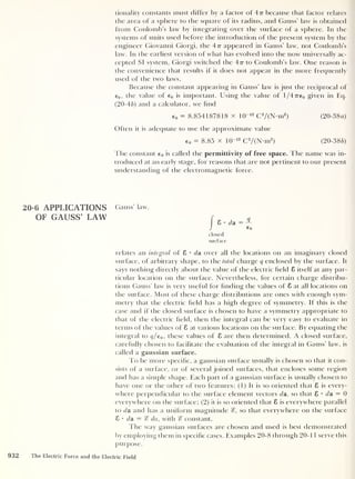
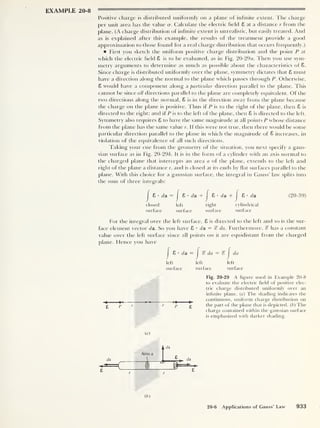
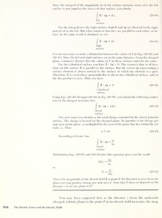
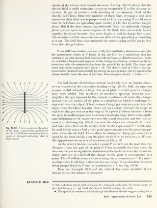
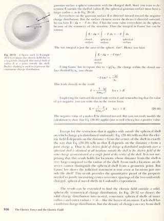
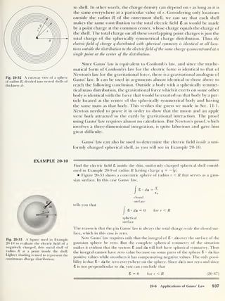
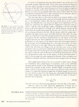
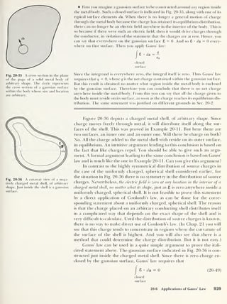
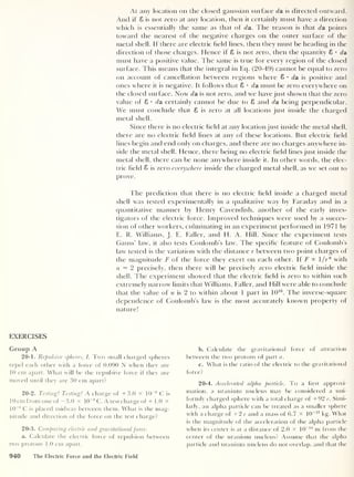
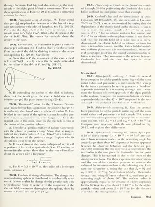

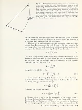
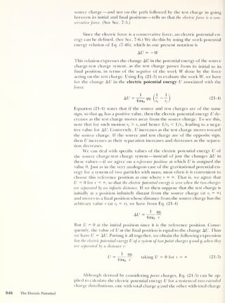
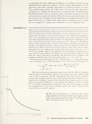
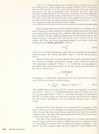
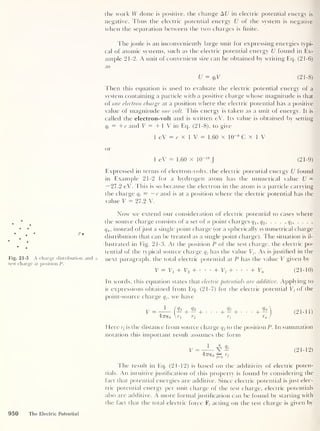
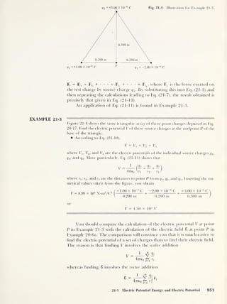
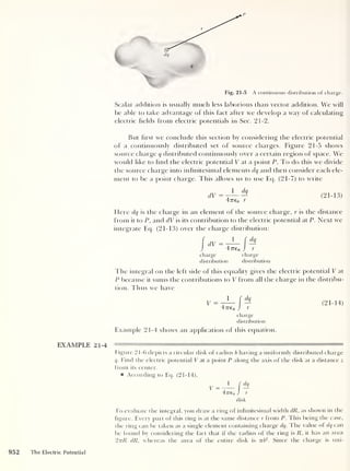
![p
Fig. 21-6 A uniformly charged, circu-
lar disk of radius b and a point P located
on its axis at distance z.
formly distributed, the ring contains a fraction dq/q of the entire charge on the disk
equal to 2 ttR dR/nb2
, its share of the entire area of the disk. Thus you have
dq 2 ttR dR
q 7zb
2
or
2qR dR
dq =
b'
The distance r from any point on the ring to P is given by the pythagorean
theorem:
r = (R2
+ z
2
)
112
As shown in the figure, the coordinate z is measured along the axis of the disk from
an origin at the disk.
Now that you have expressions for dq and r, you can write the expression for V
as
V
1 2qR dR
20/2
47re0 Jo b
2
(R2
+ z
R dR
20/2
27Te0b
2
Jo (R2
+ z
:
The limits on the integral are as written since R ranges from 0 to b over the disk.
Keeping in mind that z is a constant when the integration is performed and con-
sulting a table of integrals, you find
R dR
o (R2
+ z
2
)
1 ' 2
So you get
V =
= [(R
2
+ z
2
y2
]R=b - [(A
2
+ zT2
L=0
= ( b
2
+ z
2
)
1 '2 - z
9
2iT6ob
2
[(
b
2
+ z
2
)
1/2 - z] (21-15)
To check this result, consider the case where the distance from the disk to P is
quite large compared to the radius of the disk itself; that is, z» b. In order to
make the behavior of V as a function of z more apparent, you take advantage of the
condition z » b to expand the term ( b
2
+ z
2
)
1 /2
in Eq. (21-15). This is done by writ-
ing it in the form
/ b
2
(b
2
+ z
2
)
1 '2 = z (l +
-J
and then using the binomial expansion approximation
for z » b
b
2
i/2
1 + “o'
1 b
2
1 +
¥ z
2
Hence to a high degree of accuracy you have
1 b
2
( b
2
+ z
2
)
1/2 = z + — — for z » b
2 z
The quantity in brackets in Eq. (21-15) thus can be written
1 b
2
[( b
2
+ z
2
)
1/2 - z] =
and the equation itself reduces to
2 z
for z »
V =
47T€0 Z
for z » b (21-16a)
21-1 Electric Potential Energy and Electric Potential 953](https://image.slidesharecdn.com/robertm-220626164724-d75ac43b/85/Robert-M-Eisberg-Lawrence-S-Lerner-Physics_-Foundations-and-Appli-pdf-277-320.jpg?cb=1675858377)
![This is the same as the expression for the electric potential of a point charge q lo-
cated at the center of the disk. It is what you would expect because when z » b,
the distance from any point on the disk to the point P is equal to z within a very small
fractional error. That is, from a great distance the disk looks like a point.
The opposite extreme case, z <5c: b, is the one in which the distance from the
disk to P is quite small compared to the radius of the disk. When this is true, the
quantity z
2
in the term ( b
2
+ z
2
)
1 '2
of Eq. (21-15) can be neglected in comparison to
the quantity b
2
. Thus to a high degree of accuracy the bracket in the equation re-
duces to [(b
2
)
112 — z] = b — z, and the equation itself reduces to
V = „
q
,-
9
(b - z) for z « 6 (21-166)
2ne0 b~
Example 2 1-5 will show you how to interpret this limiting behavior of V so as to con-
clude that it is in agreement with a previously obtained result.
21-2 EVALUATION OF
ELECTRIC FIELD
FROM ELECTRIC
POTENTIAL
As has been noted, the task of calculating the electric potential V of a cer-
tain set of charges is much less difficult than calculating the electric field 8
of these source charges. The reason is that calculating V involves a scalar
summation (or integration), while calculating 8 involves a vector summa-
tion (or integration). But sometimes you really need to know 8, not V. In
such circumstances calculating 8 directly from the charge distribution by
means of Coulomb’s law often is not the easiest method. Less effort is in-
volved when the following two-step method is employed:
1. The electric potential V is calculated from the charge distribution.
2. The procedure developed immediately below is used to evaluate 8
from V.
The development is brief since it is just an application of the proce-
dure developed in Sec. 7-7 for evaluating force from potential energy.
We begin with Eqs. (7-59):
Fx
Fy
Fz
dU(x, y, z)
dx
dU(x, y, z)
dy
dU(x, y, z)
dz
The quantity U(x, y, z) is a potential energy that depends on the three coor-
dinates x, y, z, and the quantities Fx ,
Fy ,
Fz are the components along the
three coordinate axes of the force associated with the potential energy.
These relations apply to any potential energy and its associated force, in-
cluding an electric potential energy and the electric force giving rise to it.
This being the case, we consider a test charge qt
at a position whose coordi-
nates are x, y, z. The electric force exerted on it by a set of source charges
is F,, whose components are Ftx ,
Ft ,
and FL .
The electric potential energy
of the system arising from this force is U(x, y, z). The connection between
954 The Electric Potential](https://image.slidesharecdn.com/robertm-220626164724-d75ac43b/85/Robert-M-Eisberg-Lawrence-S-Lerner-Physics_-Foundations-and-Appli-pdf-278-320.jpg?cb=1675858377)
![the electric force and the electric potential energy is
Ftx =
F*.=
Ft =
8U(x, y, z)
dx
dU{x, y, z)
dy
dU(x, y, z)
dz
Let us divide both sides of each of these three equations by qt ,
the
charge on the test charge, and then use the fact that q, is a constant to make
it a part of the quantity whose partial derivative is to be evaluated. We have
Ftx
1 dU(x, y, z) d[U{x, y, z) /qP
Qt Qt dx dx
Ft.
1 dU(x, y, z) d[U(x, y, z)/qt
Qt Qt dy dy
Ft, _
1 dU(x, y, z) d[U(x, y, z)/qt ]
Qt Qt dz dz
Now the electric held 8 is defined to be
(2 1-1 la)
(21-17b)
(21-17c)
Qt
so that %x = FtJqt, %y = Ft
Jqt ,
and %z = Ft Jqt . And the electric potential V
is defined to be
V(x, y, z)
U(x, y, z)
Qt
Using these definitions in Eqs. (21-17), we obtain the desired relations
between the electric held and the electric potential:
Fig. 21-7 A uniform electric field
directed along the x axis, represented by
electric field lines and by the electric
field vector 8. Also indicated are planes
parallel to the yz plane. The electric po-
tential V has a constant value on each
plane because V depends on only x. The
value of V decreases as x increases. The
displacement vector ds shown is used
when this figure is reconsidered later.
S’*
dV(x, y, z)
dx
dV(x, y, z)
dy
dV(x, y, z)
dz
(2 1-1 8a)
(21-186)
(2 1-1 8c)
The component along a coordinate axis of the electricfield of a set ofsource charges is
given by the negative of the partial derivative with respect to that coordinate of the
electric potential of the source charges.
The simplest interpretation of Eqs. (21-18) is found in a case where the
electric held is uniform (or can be considered essentially uniform) in some
region. If we let the x axis extend along the direction of 8 in this region, as
in Fig. 21-7, then %y = 0 and — 0. Hence Eqs. (21-186) and (21-1 8c
)
read
dV(x, y, z)
dy
= 0 and
dV(x, y, z)
dz
= 0
21-2 Evaluation of Electric Field from Electric Potential 955](https://image.slidesharecdn.com/robertm-220626164724-d75ac43b/85/Robert-M-Eisberg-Lawrence-S-Lerner-Physics_-Foundations-and-Appli-pdf-279-320.jpg?cb=1675858377)
![These two relations tell us that the electric potential V has no y or z depen-
dence in the region, and so it can be written V(x). Equation (2 1-1 8a) thus
reads
3V(x)
But %x = %. Also, there is no distinction between the partial derivative and
the ordinary derivative in this case, so (hat dV(x)/dx = dV/dx. Therefore
we have
This tells us that the magnitude of the electricfield equals the magnitude of the rate
of change of electric potential with respect to position, and the direction of the electric
field is the direction in which the electric potential decreases most rapidly.
Although the italicized statement just made was obtained by consider-
ing a uniform electric held, it is valid even when the electric held varies
from point to point. The reason is that the statement concerns a relation
between the electric held and the electric potential in the immediate neigh-
borhood of some point. So it is unaffected by what these quantities do at
some other point.
Equations (21-18) can be used to evaluate the electric held of a charge
distribution from the electric potential of the distribution. Numerical re-
sults of such an evaluation can be stated by expressing the magnitude of the
electric held in units of volts per meter (V/m), as suggested by an equation
such as %x — — dV(x, y, z)/dx, instead of newtons per coulomb, as suggested
by an equation such as %x = FtJqt . That the two units are equivalent is
shown as follows:
V 1 N-m N
1
“ = 1
r = 1
T = 1
r
m C-m (. m C
Example 21-5 employs Eqs. (21-18) in evaluating the electric held at
points along the axis of a uniformly charged circular disk from the electric
potential at these points found in Example 21-4.
EXAMPLE 21-5
Evaluate the electric held at a point P along the axis of the circular disk of Example
21-4, having radius b and uniformly distributed charge q, as illustrated in Fig. 21-6.
Do this by using in Eqs. (21-18) the expression given by Eq. (21-15) for the depen-
dence of the electric potential on the axial coordinate z of point P.
Writing the electric potential in Eq. (21-15) as V(z), you have
V(z) = - [( b
2
+ z
2
)
1/2 - z]
27760 b
2
Applying Eqs. (21-18a) and (21-186) to this electric potential gives you
dV(z)
dx
= 0
and
%y
dV(z)
dy
0
These results tell you that the electric held 8 at points on the axis of the disk has no
components in directions perpendicular to the axis. This is in agreement with con-
956 The Electric Potential](https://image.slidesharecdn.com/robertm-220626164724-d75ac43b/85/Robert-M-Eisberg-Lawrence-S-Lerner-Physics_-Foundations-and-Appli-pdf-280-320.jpg?cb=1675858377)
![elusions that can be drawn from a simple symmetry argument. What is the argu-
ment?
Applying Eq. (2 1-1 Be), you obtain
= - dV(z)
=
dz
Q
2 7re 0 6
2
dz I2'77'e 0 6
1
[( b
2
+ z
2
)
1 ' 2 - z]
|
(6
2
+ z
2 )-1/2
(2z) - 1
or
sr2
q
2ne0 b
2
[1 - z(6
2
+ z
2 )- 1/2
] (21-19)
This is the required expression for the electric held.
Just as you did for Eq. (21-15) in Example 21-4, you can check Eq. (21-19) by
considering its limiting behavior. In the limit z » b (that is, when the distance
from the disk to P is large compared to the radius of the disk), you make use of the
binomial expansion approximation by writing
1 bus
(ib
2
+ z
2 )- 1 ' 2 = z”
1
2 z
2
1 b
2
z(b
2
+ z
2)-112 = 1 -
2 ^
and the quantity in brackets in Eq. (21-19) becomes
1 - z(6
2
+ z
2
)
b
l
9
Z“
So to a very good approximation you can write Eq. (21-19) as
«?2
= -—-—r for z » b (21-20a)
47re 0 z
You also can obtain the same result by applying %z
= - dV(z)/dz directly to Eq.
(21-16a). The result certainly makes sense because it says that very far away from
the disk its electric held is the same as that of a charge q located at its center.
In the limit z « b (in other words, when the distance from the disk to P is
small compared to its radius), the term z(6
2
+ z
2
)
112
in the brackets of Eq. (21-19) will
be small compared to the hrst term, 1. Hence the value of the quantity in brackets
will be nearly equal to 1, and you can write with good accuracy
= ——r, for z«b (21 -20 b)
2 Tre 0 b
Another way you can obtain the same result is to use Eq. (21-166) in the relation
%z = — dV{z)/ dz. The result is in agreement with the one obtained in Example 20-8,
where Gauss’ law was applied to evaluate the electric held by a plane of infinite ex-
tent, carrying the uniform charge per unit area cr. According to Eq. (20-45), its
value is % = cr/2e0 . For z <5C b the edges of the uniformly charged disk are so far
away from the point P, compared to the distance from the disk to P, that they might
as well be inhnitely far away. That is, the fact that the disk is of finite extent should
make no difference to the value of the electric held. The charge per unit area on the
disk carrying charge q is cr = q/vb2
,
since rrb
2
is its area. Thus if we drop the sub-
script z in Eq. (21-206) to conform to the notation used in Eq. (20-45), the former can
be written % = o-/2e0 , in agreement with the latter.
Equations (21-20a) and (21-206) show that very near the charged disk the elec-
tric held along its axis has a magnitude independent of the distance from the disk,
whereas far from the disk this held decreases in inverse proportion to the square of
21-2 Evaluation of Electric Field from Electric Potential 957](https://image.slidesharecdn.com/robertm-220626164724-d75ac43b/85/Robert-M-Eisberg-Lawrence-S-Lerner-Physics_-Foundations-and-Appli-pdf-281-320.jpg?cb=1675858377)

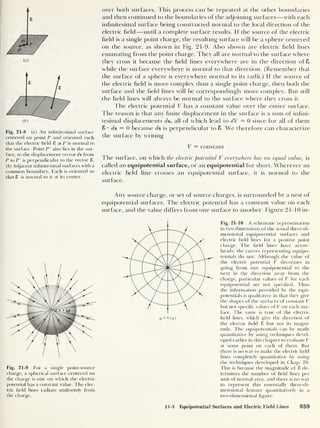
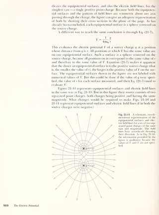
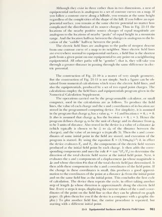
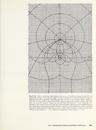
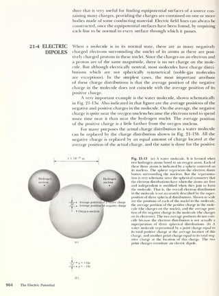
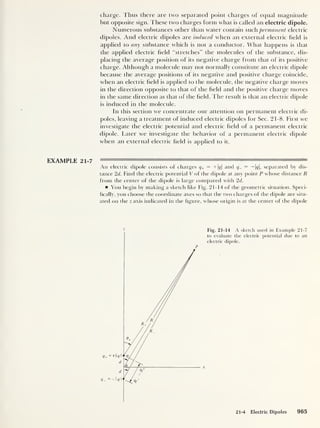
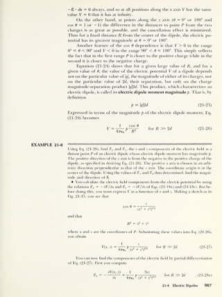
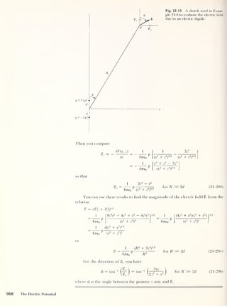
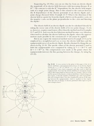
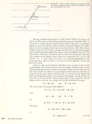
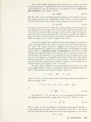
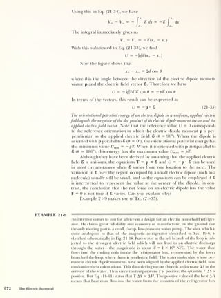
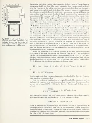
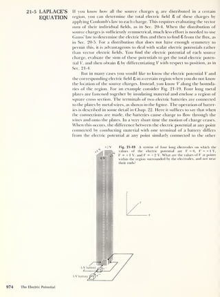
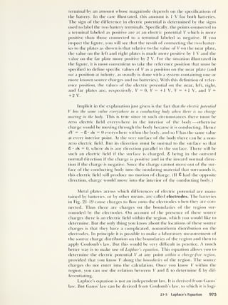
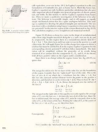
![coordinate has the value x. For this face the outward surface-element
vector cla points in the negative x direction, and so it can be written da =
— da x. Thus here we have 8 •
da = («? x x + %vy + %zz) •
(
— da x) =
— %x da. The integral is
j
8 •
da = — J
%x da
face dy dz face dy dz
at x at x
Thus we have
|
8 •
da = — {
<
&x )x dy dz
face dy dz
at x
where (%x) x is the value of %x at the center of the face at coordinate x.
The sum of the integrals of 8 • da over the pair of faces of area dy dz is
g • da + 8 • da = (
%
x) x+dx dy dz - {%x)x dy clz
face dy dz face dy dz
at x + dx at x
{J$x)x+dx - (%x)x] dy dz
The quantity in brackets is the difference between the values of %x at the
centers of the pair of faces of the infinitesimal cube. Since the two faces are
only an infinitesimal distance dx part, the quantity can be expressed as the
rate of change of %x with respect to x at the center of the cube times the dis-
tance dx between the faces. That is,
(%x)x+dx - (%x)x = dx
We employ partial derivative notation because the x component of the elec-
tric field, %x ,
may depend on any of or all the independent variables x, y, z,
but we want the rate of change with respect to x only. Using this relation,
we obtain
f f d
%
I 8 • da + I 8 • da — dx dy dz (21-37a)
face dy dz face dy dz
at x + dx at x
In completely similar ways, we can obtain
and
|
8 • da +
J
8 • rfa =
d^y
„ dy dx dz
dy
(21-376)
face dx dz face dx dz
at y + dy at y
j
6 • da + Cr>
a.p II
d%z
_ dz dx dy
dz
7 (21-37c)
face dx dy face dx dy
at z + dz at z
If we now add Eqs. (21-37a), (21-376), and (21-37c), the left side of the
equality that is produced is just the integral of 8 • da over the closed sur-
face formed by all six faces of the cube. So the addition yields
8 • da = ^dx dy dz + ^dy dxdz+^
dx
J
dy
J
dz
dz dx dy
closed
surface
977](https://image.slidesharecdn.com/robertm-220626164724-d75ac43b/85/Robert-M-Eisberg-Lawrence-S-Lerner-Physics_-Foundations-and-Appli-pdf-301-320.jpg?cb=1675858377)
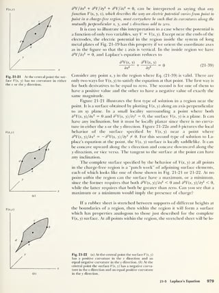
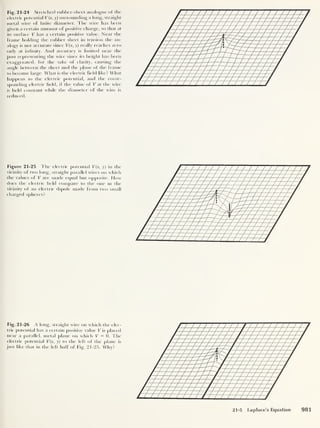
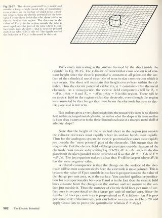
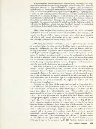
![true independent of the inclination of the tangent to either surface at its
central point. Thus Laplace’s equation says, in effect, thatt/ic value ofV(x, y)
at any point in a charge-free region must be the average of its values atfour symmet-
rically disposed, nearby surrounding points. Example 21-10 makes use of this
property of the electric potential.
This basic property can also be obtained directly from Laplace’s equation, Eq.
(21-39),
d
2
V(x, y) d
2
V(x, y)
dx2 +
dy2
by applying to it the definition of a partial derivative. The first partial derivative
with respect tox ofV(x, y) at the point x, y can be defined in terms of the approxi-
mation
dV(x, y) V(x + Ax/2, y) — V(x - Ax/2, y)
dx Ax
(21-40)
with the understanding that the approximation is better as the separation Ax
between the two symmetrically disposed points at which V(x, y) is evaluated be-
comes smaller. In the limit Ax —» 0, this is completely equivalent to a definition
involving the more familiar expression [V(x + Ax,y) -V(x,y)]/Ax. But Eq.
(21-40) has the advantage of providing a more accurate approximation to
dV (x, y)/dx for any value of the finite quantity Ax. The second partial derivative
with respect to x can be expressed similarly by using Eq. (21-40) to compute d/dx
of dV (x, y)/dx. That is,
d TdV(x,y)~
dx L dx
[V((x + Ax/2) + Ax/2, y)
- V ((x - Ax/2) + Ax/2, y)]
Ax Ax
[V((x + Ax/2) — Ax/2, y)
— V((x - Ax/2) - Ax/2, y)]
Ax Ax
or
d
2
V(x, y) __
V(x + Ax , y)
— 2V (x , y)
+ V(x - Ax , y)
dx 2 “ (Ax) 2
Similarly, we have for the second partial derivative with respect to y
(21-41)
d
2
V(x, y) V(x, y + Ay) - 2V(x, y) + V(x, y - Ay)
^ ^
dy 2
~
(Ay) 2 1 ' J
Setting Ax = Ay in Eqs. (21-40) and (21-41) and then substituting into Eq. (21-39),
we find
V(x + Ax, y) + V(x Ax, y) + V(x, y + Ay) + V(x, y - Ay) - 4V(x, y)
(Ax) 2
for Ax = Ay
Then multiplying through by (Ax) 2
and transposing, we obtain
V(x, y)
V(x + Ax, y) + V(x - Ax, y) + V(x, y + Ay) + V(x, y - Ay)
4
for Ax = Ay (21-43)
This approximate equality becomes exact when Ax and Ay go to zero. The right
side of this equation is precisely the average of the values of the function V at the
four symmetrically disposed points surrounding the point x, y. The left side of the
equation is the value of V atx, y. So the equation makes the same statement as the
italicized sentence immediately preceding this small-print material, which was
based on the geometry of Figs. 21-21 and 21-22. If V is a function of the three coor-
984 The Electric Potential](https://image.slidesharecdn.com/robertm-220626164724-d75ac43b/85/Robert-M-Eisberg-Lawrence-S-Lerner-Physics_-Foundations-and-Appli-pdf-308-320.jpg?cb=1675858377)
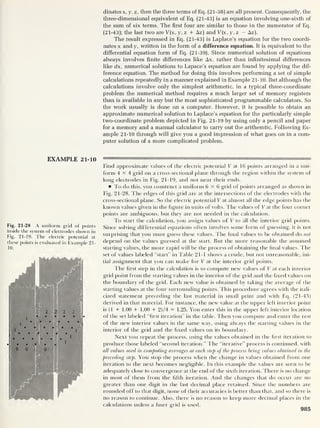
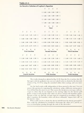
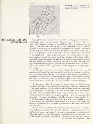
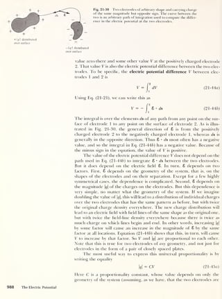
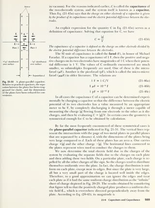
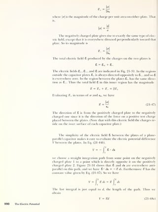
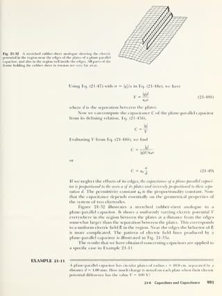
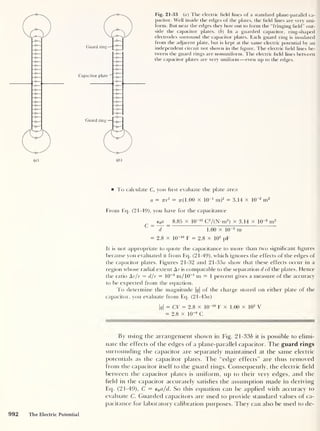
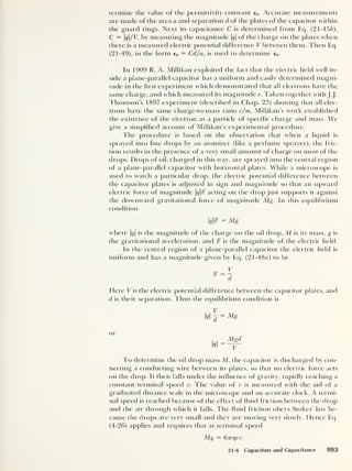
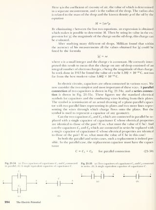
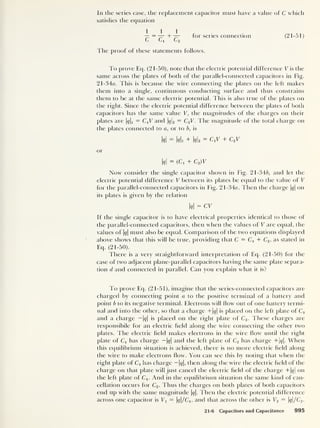
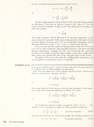
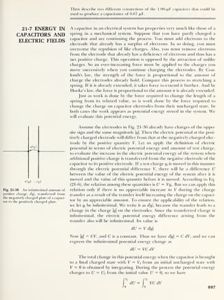
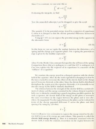
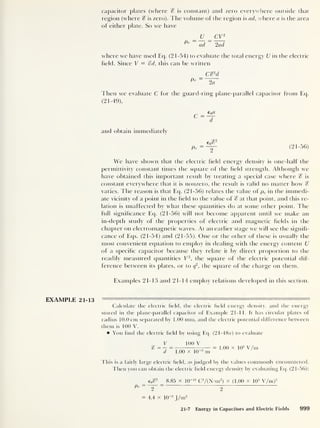
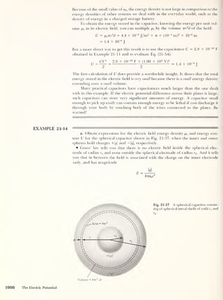
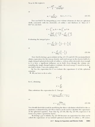
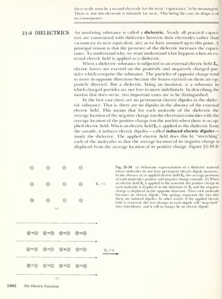
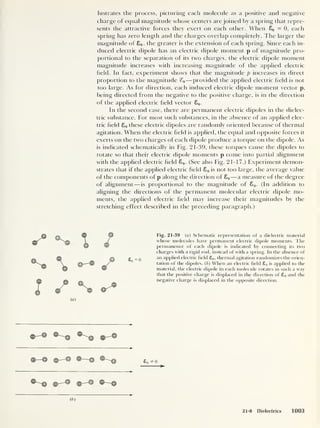
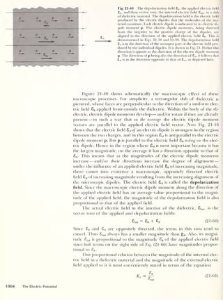
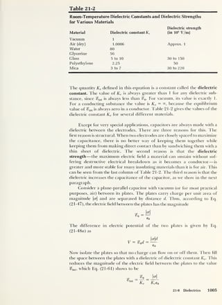
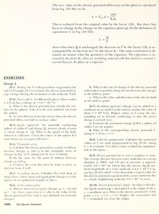
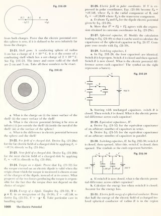
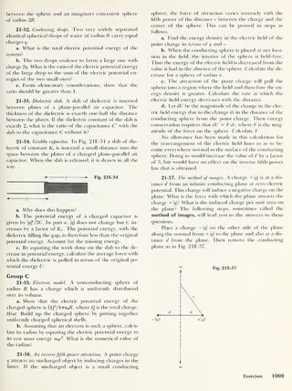
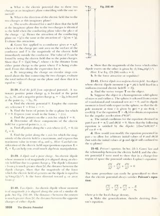
![b. Determine the electric field 8. and charge density
p, associated with the electric potential
V(x, y, z) = ae
~bz
2
where a and b are constants.
21-43. The consequences of symmetry. A cubical box has
aluminum faces which are mechanically joined by narrow
insulating spacers which serve as the edges of the cube.
The interior of the box is charge-free. The six faces of the
cube are connected to six different batteries which main-
tain them at the following electric potentials: 5, 15, — 10,
30, 45, and - 25 V.
a. Without using any complicated numerical proce-
dure, determine the electric potential at the center of the
cube. Justify your method.
b. For which object(s) among the following could a
similarly simple means be used to determine the electrical
potential at the geometrical center? (In each case, there
are no interior charges, and various parts of the surface
are held at various given electric potentials.)
(i) a hollow, regular tetrahedron
(ii) a hollow, noncubical rectangular parallelepiped
(iii) a hollow spherical shell
21-44. A charged sheet, I. An infinite sheet containing a
position-dependent charge per unit area lies in the xy
plane; its electric potential is given by V(x,y, 0) = V0 cos(kx).
a. Find the electric potential V(x, y, z) in the charge-
free region on both sides of the infinite sheet. Hint: As-
sume that V{x, y, z) = /(z) cos(foc) and that V —» 0 for z —
»
00 . Why should there be no y-dependence in V(x, y, z) for
z f 0?
b. Evaluate the electric field 8 (x, y, z) for z f 0.
c. Show that the magnitude of the electric field de-
pends only upon z.
21-45. A charged sheet, II. Apply Gauss’ law to find the
charge per unit area cr(x, y) of the sheet described in Exer-
cise 21-44.
Numerical
21-46. Field lines and equipotentials, I. Run the field
lines and equipotentials program to trace a representative
set of electric field lines and equipotential curves for two
charges whose value and locations are: q^ = + 1 (in C) at
x = 0 and z = 0; q2 = + 2 (in C) at x = 0 and z = 5 (in
cm). 1 his work is quite time-consuming if carried out on a
programmable calculator. (But there is no tedium if you
use a computer with a graphic display.) So use values of As
and n which are, respectively, twice as large and twice as
small as those used in Example 21-6. in order to reduce
the time required (unless you use a graphic display com-
puter). Also, evaluate V for each equipotential. Compare
your results with those displayed in Fig. 21-11, and com-
ment on the differences.
21-47. Field lines and equipotentials, II. Run the field
lines and equipotentials program to trace a representative
set of electric field lines and equipotential curves for two
charges whose values and locations are: q1 = + ] (in C) at
x = 0 and z = 0; q2 = — 2 (in C) at x = 0 and z = 5 (in
cm). Also evaluate V for each equipotential. Compare
your results with those displayed in Fig. 21-12, and com-
ment on the differences. The remarks made in Exercise
21-46 about the time required for the calculations apply
here.
21-48. Laplace’s equation, I.
a. This exercise requires the use of a small computer.
Write a program for carrying out an iterative solution of
Laplace’s equation. Follow the lines established by Ex-
ample 21-10, but allow for a more flexible choice of the
number of grid points and for the specification of the val-
ues of V at the boundaries. Test the program by repeating
the calculation in the example, recording the time re-
quired to obtain convergence to two decimal places.
b. Choose a different set of initial values of V at the
interior grid points. Specifically, choose V = 0 at each of
these points. Repeat the calculation, and show that the
same results are obtained. Also record the time required
to obtain the results. Compare the time required for the
two calculations, and explain what the comparison shows.
21-49. Laplace’s equation, II. Run the Laplace’s equa-
tion computer program as in Exercise 21-48 until you ob-
tain convergence to three decimal places. Record your re-
sults. Then repeat the calculation with a grid in which the
spacing of the grid points is halved along both the x and y
axes. Record your results, but only at the positions of the
initial set of grid points. Continue this process, repeatedly
halving the grid point spacing, until the calculation con-
verges with respect to grid point spacing to three-
decimal-place accuracy. When the convergence is
achieved, the results of the numerical calculations will be
identical to this accuracy with the results of analytical cal-
culations.
21-50. Laplace’s equation, III.
a. Apply the Laplace’s equation computer program
written in Exercise 21-48 to find values of V at points in-
side a set of three adjacent long electrodes extending in
the z direction, whose intersections with the xy plane form
a triangle with two perpendicular sides of equal length.
The values of V on the two perpendicular electrodes are
V = 0 and V — + 1 V. The value on the third electrode is
V = + 2 V.
b. Explain briefly the difficulty that arises if the trian-
gle does not have two perpendicular sides of equal length,
and what you would do to handle the difficulty. Laplace’s
equation does not have analytical solutions for the elec-
trode systems considered in either part of this exercise.
Exercises 1011](https://image.slidesharecdn.com/robertm-220626164724-d75ac43b/85/Robert-M-Eisberg-Lawrence-S-Lerner-Physics_-Foundations-and-Appli-pdf-335-320.jpg?cb=1675858377)
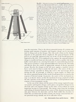
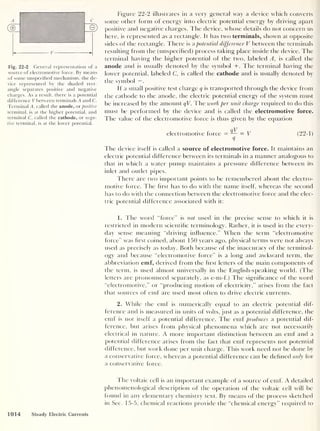
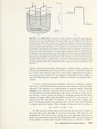
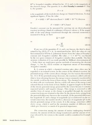
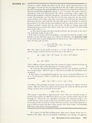
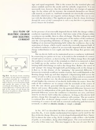
![Lower
Higher '<!
potent ]
Fig. 22-5 A tube of flow of electric charge. The streamlines, called
current lines, are denoted by dashed curves. Their sense is conven-
tionally from higher to lower electric potential, and they are every-
where tangent to the local electric held vector £ . However, the
charge motion has the same sense as the current only if the charge is
positive. Negative charge moves in the opposite sense, from lower to
higher electric potential. By definition of a tube of flow, no charge
passes through the walls of the tube. Since the tube contains no
sources or sinks of charge, the current passing through the surface
M must be equal in the steady state to the current passing through
the surface N.
cause of a variation in the size of the pipe. In the case of flow of electric
charge, the same effect may result from a variation in the size of the wire
carrying the flowing charge.
For water flow, we can draw an imaginary surface across the tube of
flow at any location and use Eq. (16-35) to define the mass flux
dm
dt
(22-5)
The mass flux is thus the mass m of fluid which passes across the surface
per unit time t. We do a completely analogous thing for the flow of electric
charge in a conductor. I he electric charge flux is almost always called elec-
tric current, defined to be the amount of electric charge q passing per unit
time through an imaginary surface (such as M in Fig. 22-5). The symbol i is
universally used for electric current. Thus we have, by definition,
i
dq
dt
( 22-
6)
The unit of electric current must be coulombs per second. This very impor-
tant unit is given the name ampere (A) after the French physicist Andre
Marie Ampere (1775-1836), who was one of the founders of the theory of
electromagnetism. The ampere is thus related to the coulomb by the ex-
pression
1 A = 1 C/s (22-7)
The current i is a signed scalar. We often have used the term “signed
scalar” to denote a vector in one dimension. But the current is not a vector,
even when it describes the flow of charge in a long, thin wire. This is be-
cause of an essential aspect of any flow of charge: it must always flow in an
electric circuit, or closed pathway. Such a closed pathway cannot exist in
one dimension; at best, the long, thin wire is only a part of a complete cir-
cuit. Nevertheless, a current must always have a sense, and it is this sense
that is denoted by the sign of i. Even in the simplest loop, consisting of a
22-2 Flow of Electric Charge and Electric Current 1019](https://image.slidesharecdn.com/robertm-220626164724-d75ac43b/85/Robert-M-Eisberg-Lawrence-S-Lerner-Physics_-Foundations-and-Appli-pdf-343-320.jpg?cb=1675858377)
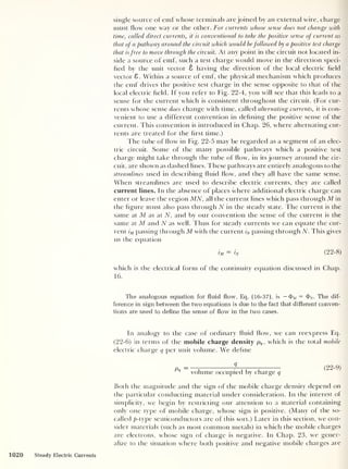
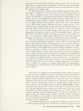
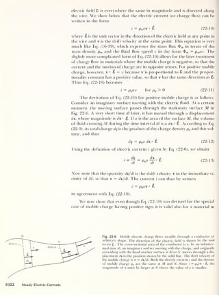
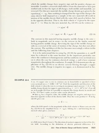
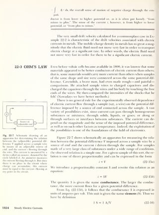

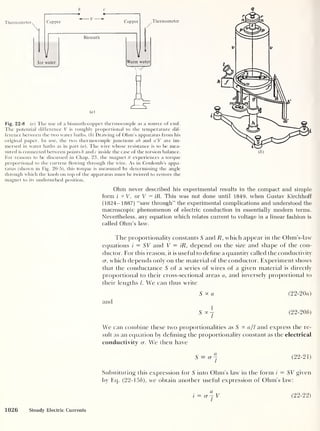
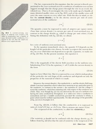
![Table 22-1
Electrical Conductivity, Resistivity, and Temperature Coefficient for
Various Metals and Alloys
(Reference temperature t 0 = 20°C)
Metal o-0 (in 10H
S/m) p0 (in 10 8
ft-m) a (in °C-1
)
Silver 62.9 1.59 0.0058
Copper (hard drawn) 56.47 1.771 0.0038
Gold 41.0 2.44 0.0034
Aluminum 35.41 2.824 0.0039
Tungsten 18 5.6 0.0045
Iron 10 10 0.005
Lead 4.5 22 0.0039
Bismuth 0.83 120 0.004
Mercury 1.0440 95.783 0.00089
Brass 14 7 0.002
Manganin 2.3 44 0.00001
Constantan 2.0 49 0.00001
Nichrome 1.0 100 0.0004
slowly with increasing temperature, and the conductivity decreases corre-
spondingly. It is conventional to express the resistivity as a polynomial
series in the Celsius temperature t. However, it is usually not necessary to
consider terms beyond the term linear in temperature. Given the resistivity
pn at some reference temperature t0 ,
it is usually sufficiently accurate to
express the resistivity p at some other temperature t in the form
p = Po[l + a(t - <0 )] (22-26)
The empirical constant a is called the temperature coefficient of resistiv-
ity. The reference temperature t0 ,
at which the resistivity has the value p0 ,
is
usually (but not always) taken to be t0 = 20°C. Table 22-1 gives values of the
conductivity cr0 and the resistivity p0 at t = t0 and the temperature coeffi-
cient a for various metals and alloys.
In general, “good" metals have high conductivities. By “good" metals is
meant those which have most of or all the classical metallic properties, such as
ductility and luster, and clearly metallic chemical properties, such as exclusively
positive valences. Roughly speaking, metals which possess these properties in
lesser degree are not such good conductors as those which possess them in greater
degree. Consider the extreme cases in Table 22-1. Silver is shiny and highly duc-
tile and always has a chemical valence of + 1 or +2. It has the highest conducti-
vity of all metals at room temperature. Bismuth is dull in appearance and rather
brittle and combines chemically in a variety of complicated ways; it is a poor con-
ductor of electricity, as metals go.
At temperatures far below room temperature, the behavior of metals is both
more complicated and more diverse. Most dramatic among the metals are those
called superconductors. While superconducting metals usually have relatively
low room-temperature conductivities, there is a critical temperature Tc , character-
istic of each, below which its conductivity abruptly becomes infinite. That is,
once started in a loop of a superconducting metal, a current will continue
flowing indefinitely, provided the temperature is kept below Tc . The highest criti-
cal temperature for a pure metal is that for niobium, for which Tc = 8.9 K. Super-
conductors have found important application in the manufacture of high-field
22-3 Ohm’s Law 1029](https://image.slidesharecdn.com/robertm-220626164724-d75ac43b/85/Robert-M-Eisberg-Lawrence-S-Lerner-Physics_-Foundations-and-Appli-pdf-353-320.jpg?cb=1675858377)
![electromagnets, and they may be used in the near future in long-distance electric
power transmission and in computer memories.
Alloys have much lower conductivities than pure metals, and their tempera-
ture coefficients of conductivity are generally much smaller than those of pure
metals. We discuss some reasons for this in Sec. 22-5.
In Examples 22-3 and 22-4, Ecj. (22-27) and Ohm's law are applied to
situations of practical significance.
EXAMPLE 22-3 m —
—
William Siemens proposed in 1860 that the standard of resistance be a column of
pure mercury exactly 1 m long and 1 mm2
in cross-sectional area, held at a tempera-
ture of exactly 0°C. What is the resistance of this proposed standard in ohms? How
long should the mercury column be if its resistance is to be 1.0000 fl?
Inserting the values of the resistivity p0 and the temperature coefficient a for
mercury from Table 22-1 into Eq. (22-26), you have
p(0°C) = 95.783 x 10“8
fl-m x [1 + 0.00089 “C"1
x (0°C - 20°C)]
= 94.078 x 10
-8
fl-m
And using Eq. (22-256), R = pl/a ,
you obtain
R =
94.078 x 10“8
fl-m x 1 m
1 X 10
-6
nr
0.94078 f!
for a column 1 m long. II the resistance is to be 1.0000 fl, the length of the column
should be
,
RA 1.0000 a x 1 x 10
-6
m2
, nnan
l
= = — „
= 1.0630 m
p 94.0/8 x 10 8
a-m
For many years a mercury column 1.06300 m long, containing a mass of mer-
cury equal to 14.4521 g and a constant cross-sectional area (which, given this
mass, turns out to be very close to 1 mm2
), was the primary standard of resistance,
the international ohm. At a time when means of measuring mass and length were
more accurate than those for voltage and current, this definition was useful for its
high precision and reproducibility. However, it lost its usefulness when this situa-
tion ceased to exist. Today there is no primary standard ohm. Rather, the ohm is
defined to be 1 V/A, as we have done in Eq. (22-19). However, excellent secondary
standards are available, which are stable and convenient to use.
The copper wire of Example 22-2 carries its maximum rated current i
= 15.0 A.
Find the magnitude of the internal electric field which drives the current. The tem-
perature of the wire is 50°C.
Using Eq. (22-24), j
= crcf, you can express the electric-field magnitude in the
form % — j/cr. You can evaluate the current density j by using Eq. (22-23), j = i/a.
Using the value of a from Example 22-2, you have
15.0 A
2.08 x 10“6
in
2
= 7.21 x 10
6
A/m2
To find the conductivity cr, you can use Eq. (22-26),
p = po[l + a(t - to)]
to obtain the value of the resistivity at 50°C and then write Eq. (22-25) in the form
a = 1/p to evaluate the conductivity at the same temperature. Or else you can use
1030 Steady Electric Currents](https://image.slidesharecdn.com/robertm-220626164724-d75ac43b/85/Robert-M-Eisberg-Lawrence-S-Lerner-Physics_-Foundations-and-Appli-pdf-354-320.jpg?cb=1675858377)
![Eq. (22-26) to derive a general expression for the temperature dependence of o
You have
cr = p' 1 = po
!
[l + a(t - t0 )]
_1
= cr0[l + a(t - t0 )]
_1
Since a rough calculation using the value of a from Table 22-1 shows you that
a(t — t0)
« 1, you can use the mathematical approximation (1 + x)
n — 1 + nx,
which is valid for any exponent n if x <5C 1. So you obtain the general result
cr = <r0[l - a(t
- t0 )] (22-27)
Inserting the numerical values, you find the result
a = 56.47 x 10⁶
S/m x [1 - 0.0038 “C"1
x (50°C - 20°C)] = 50.0 x 10⁶
S/m
Finally, you use the values ofj and cr to calculate
j _ 7.21 x 10
6
A/m2
cr 50.0 X 10
6
S/m
= 0.144 V/m
The result of Example 22-4, with a potential difference of only 0. 144 V
between two points 1 m apart is typical of metal wires carrying ordi-
nary currents.
Up to this point we have discussed only uniform current densities in
cylindrical wires. In this important special case, the current i, the current
density j, and the cross-sectional area a may all be dealt with in terms of
magnitudes only. The direction of the current lines is everywhere along the
wire, and a plane of fixed cross-sectional area can always be drawn normal
to the current lines. Since the current density is uniform, it can be defined
simply as j = i/a. What is more, the electric field has the same magnitude
c? everywhere along the wire.
But this is not always the case. Consider, for example, the disk-shaped
conductor shown in Fig. 22-10. A wire of a material having a much higher
conductivity than that of the disk supplies current to the small high-
conductivity core at its center. Around the edge of the disk is wrapped a
band of the same high-conductivity material. Thus the core and the edge
may be considered as equipotential regions; the potential difference
between them is distributed in some way through the disk. How can we des-
cribe the current through the disk? Since charge cannot accumulate any-
where in the disk, the current flowing out through band B must be equal to
that Howing in through core A. And the same current must pass through
the disk. Specifically, all the current must pass through any closed “hoop”
Fig. 22-10 A disk-shaped conductor. Current flows through the
disk from A to B. In doing so, it must pass through the cylindrical
closed surfaces D and£, and also through the irregular closed sur-
face C. Some current lines are denoted by arrows. By symmetry,
they must be straight, radial lines.
22-3 Ohm’s Law 1031](https://image.slidesharecdn.com/robertm-220626164724-d75ac43b/85/Robert-M-Eisberg-Lawrence-S-Lerner-Physics_-Foundations-and-Appli-pdf-355-320.jpg?cb=1675858377)
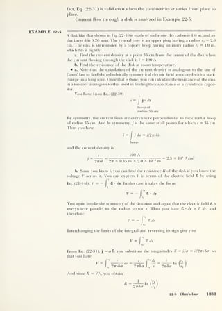
![field. The reason is that the field has a direct effect on the drift velocity
only. As long as the drift velocity is very small compared to the random ve-
locities of the individual electrons (and you have seen that it is typically only
10
-8
as large), the distance they cover per unit time is governed essentially
by the latter. And since the collisions made by the electrons are with objects
having some average separation, a change in the electric field has negligible
influence on the time required, on the average, for an electron to pass from
one collision to the next. It follows that the mean scattering time t is indeed
independent of %, and therefore the entire quantity Ne2
T/me on the right
side of Eq. (22-43a) is a constant independent of Thus our model sa-
tisfies Ohm’s law.
Note that the charge — e on the charge carriers (which we assumed from the
beginning to be electrons) enters Eq. (22-43a] only as a square, e
2
. Thus the valid-
ity of Eq. (22-43a )
does not depend on the sign of the charge carriers. If Ohm’s law
is obeyed by some substance other than a metal, where the charge carriers are not
electrons but other particles with a charge-to-mass ratio q/m, the conductivity is
given by the expression
Nq 2
r
(22-43b)
m
We can explore how well this rather crude picture of electrons in a
metal conforms to reality by making comparisons with experimental re-
sults. Solving Eq. (22-43a) for the mean scattering time gives
crrne
~N?
(22-44)
We have no direct way of measuring r and thus checking the theory against
experiment. However, an electron moving with the random speed urms
makes a collision, on the average, every time it travels a distance A given by
A = urmsT (22-45)
This distance is called the mean free path. [As was pointed out in the first
small-print section following Eq. (22-36), the drift speed is very small com-
pared to the random speed. So it does not significantly affect the relation
between collision time and collision distance.] For an ideal gas, Eq. (18-53)
gives for the root-mean-square random speed
(5 kT
1/2
tW = —— (22-46)
me )
where k is Boltzmann’s constant and T is the absolute temperature. Substi-
tuting Eqs. (22-44) and (22-46) into Eq. (22-45), we obtain
/3 kT 1/2 <rme
^ me ) Ne2
or
A = ^ (3 kTme Y
12
(22-47)
If the ‘Tree-electron" model we have developed is to be physically mean-
ingful. this value of the mean free path must be comparable to the distance
between ions in the metal, since we have tentatively assumed that the free
22-5 The Microscopic Basis of Electric Resistance 1041](https://image.slidesharecdn.com/robertm-220626164724-d75ac43b/85/Robert-M-Eisberg-Lawrence-S-Lerner-Physics_-Foundations-and-Appli-pdf-365-320.jpg?cb=1675858377)
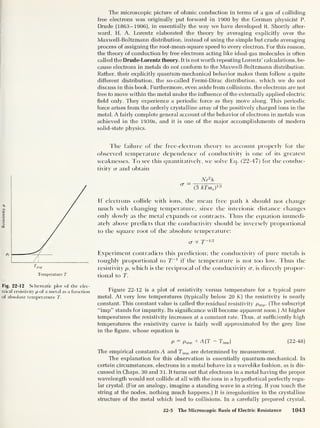
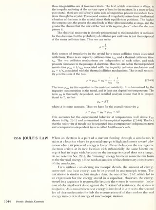
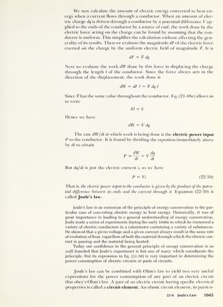
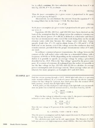
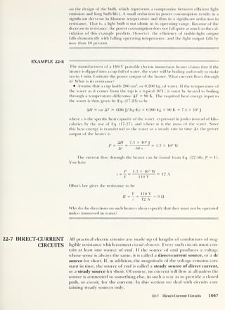
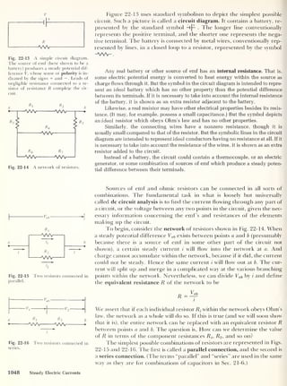
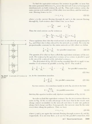
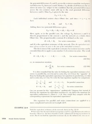
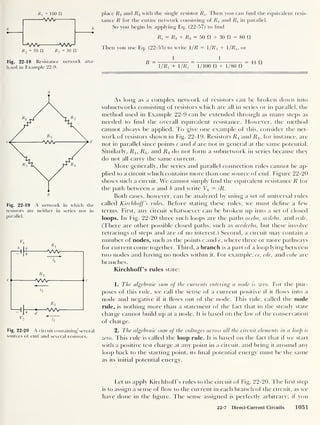
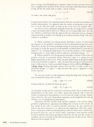
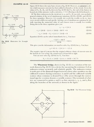
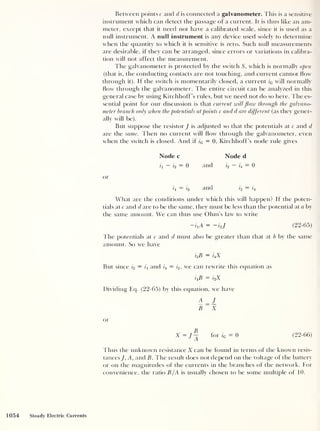
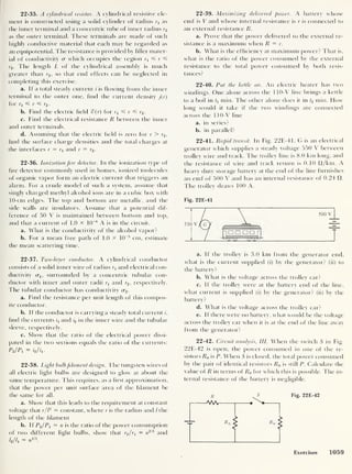
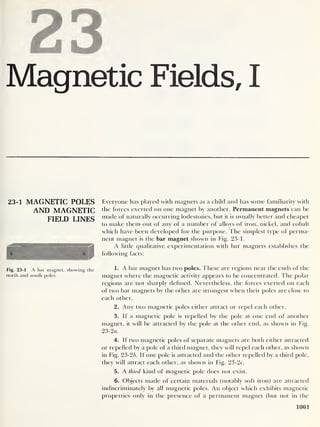
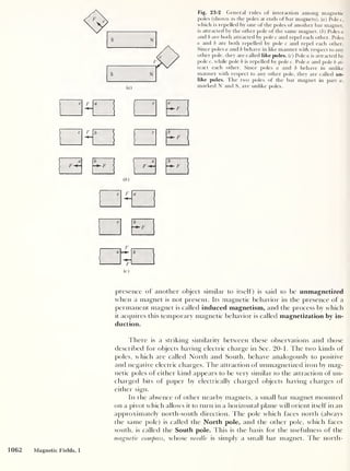
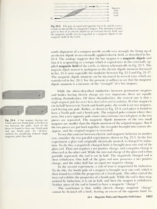
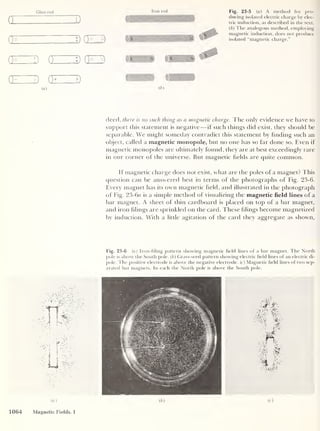
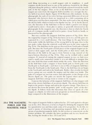
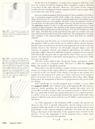
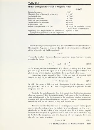
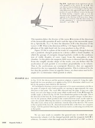
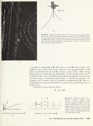
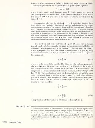
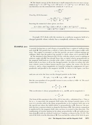
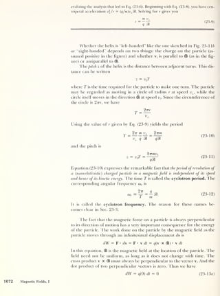
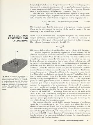
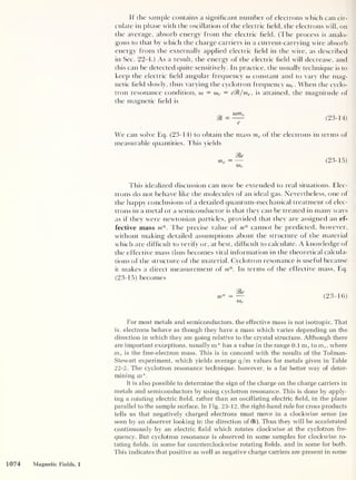
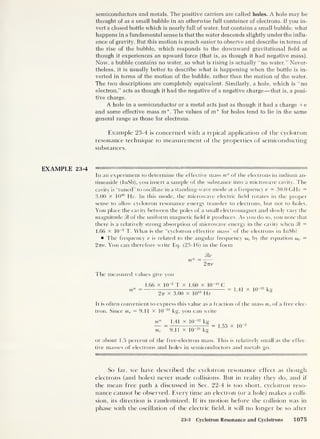
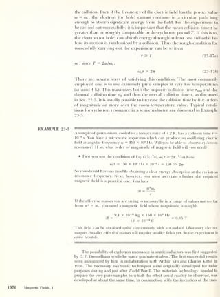
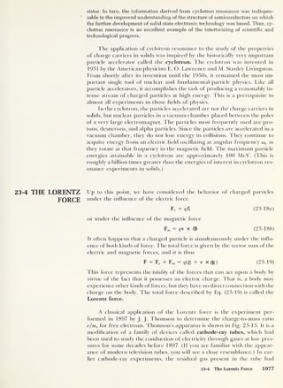
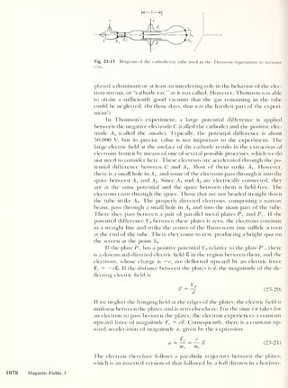
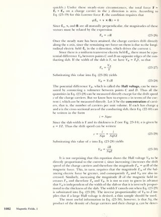
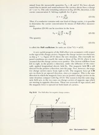
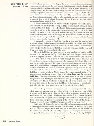
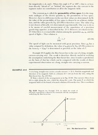
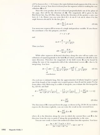
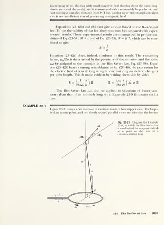
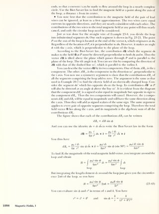
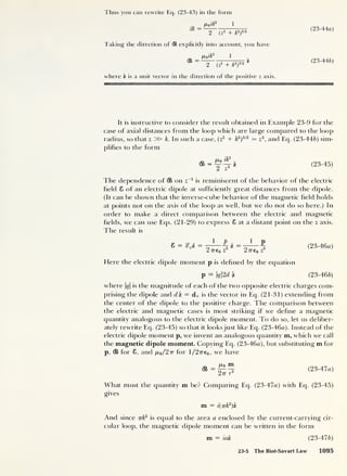
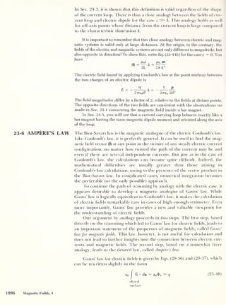
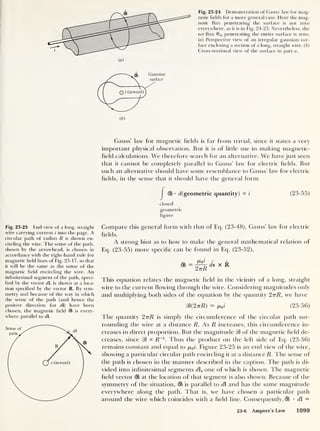
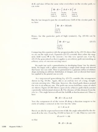
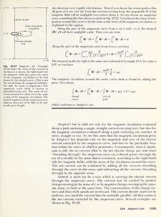
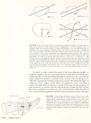
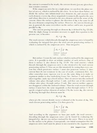
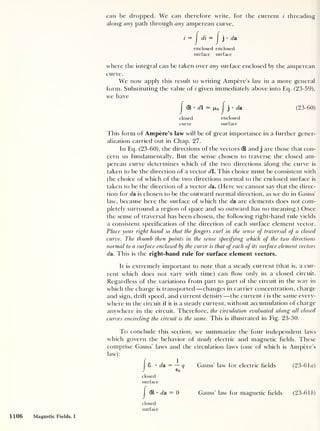
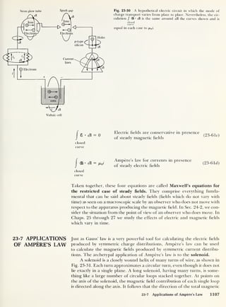
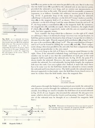
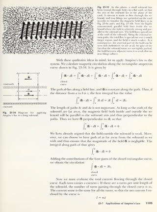
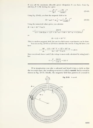
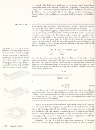
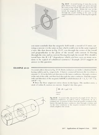
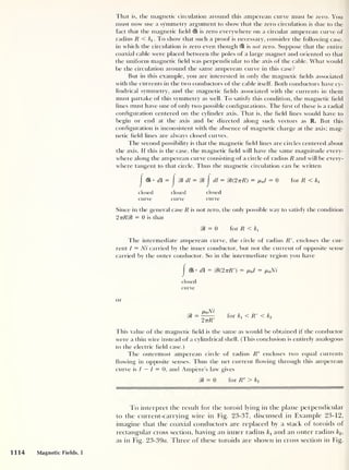
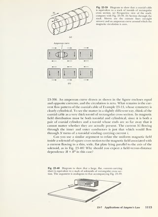
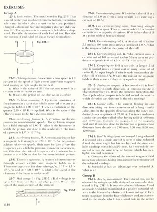
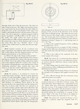
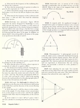
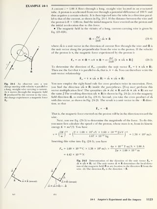
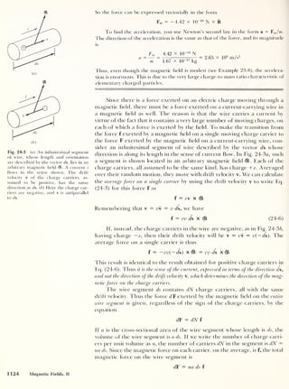
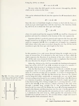
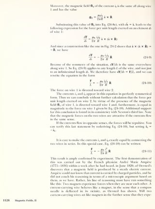
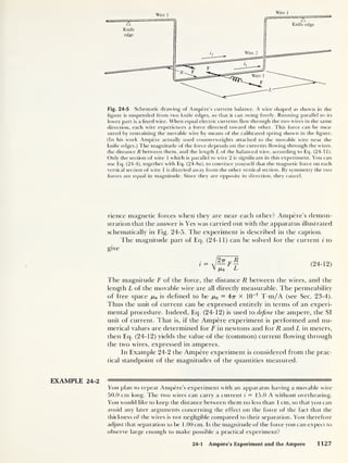
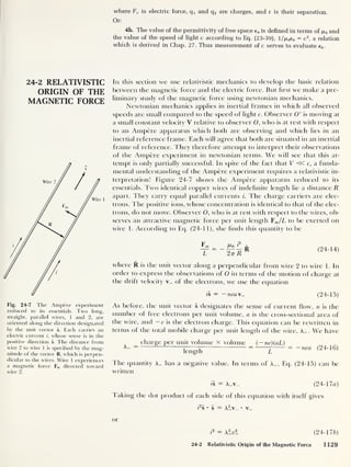
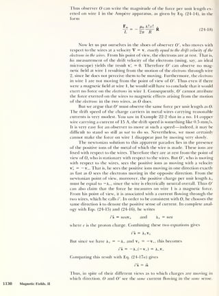
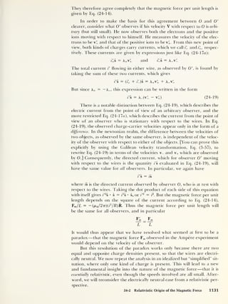
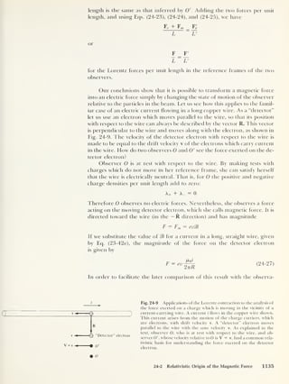
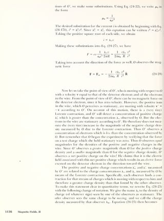
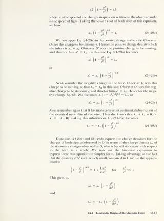
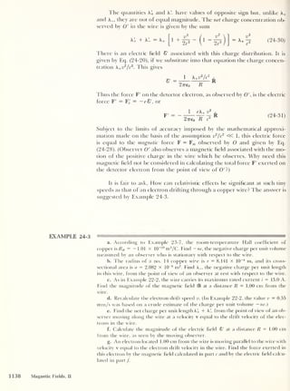
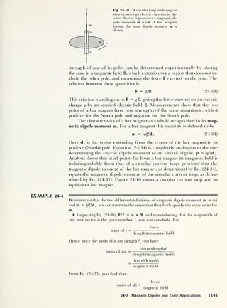
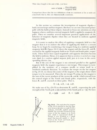
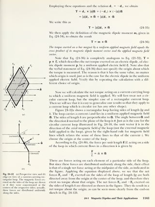
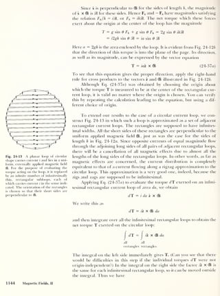
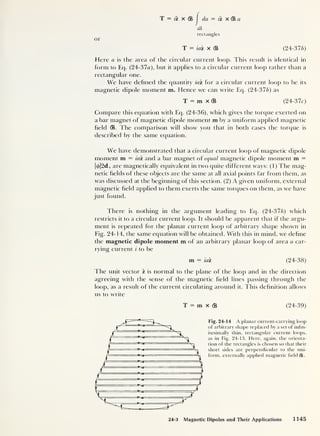
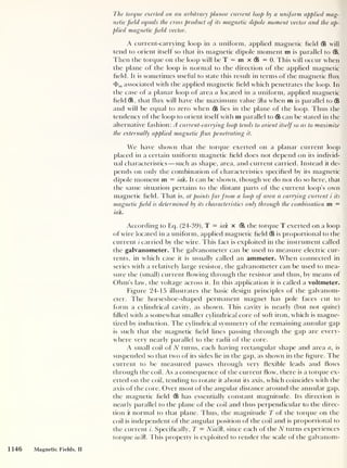
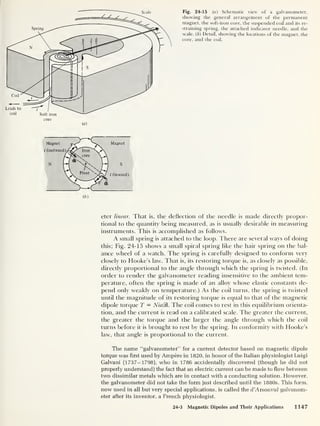
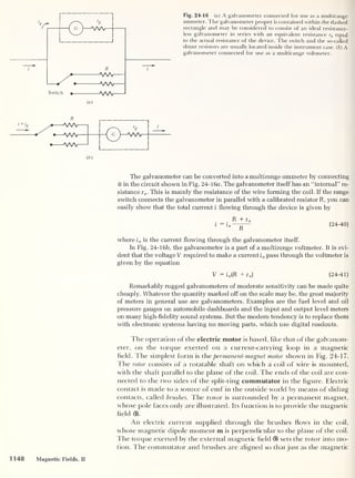
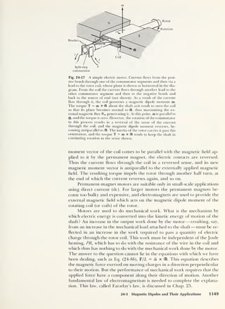
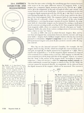
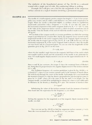
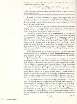
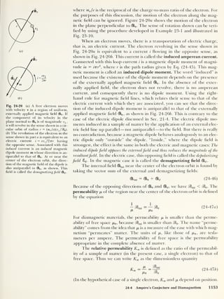
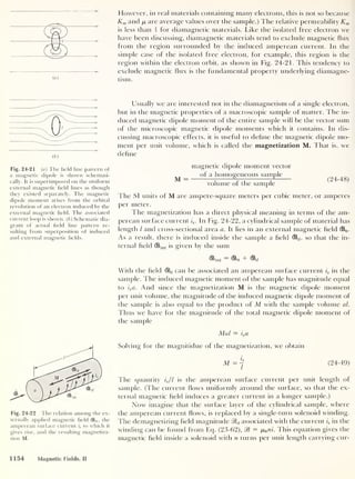
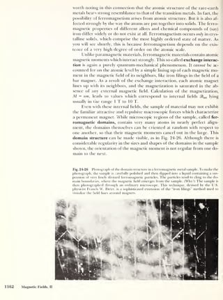
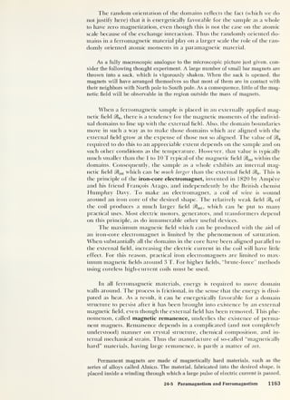
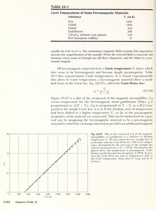
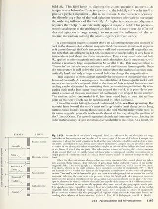
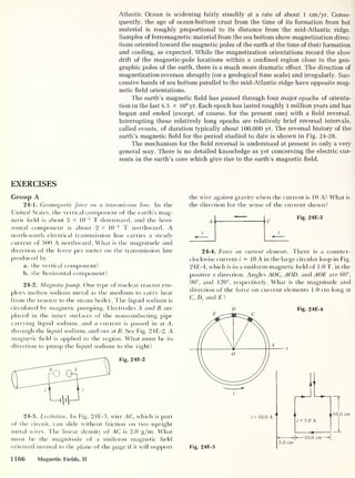
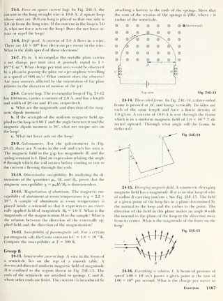
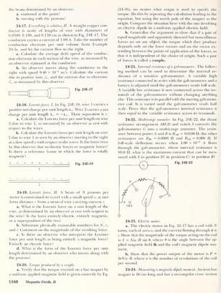
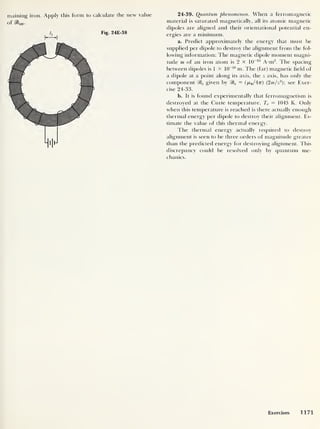
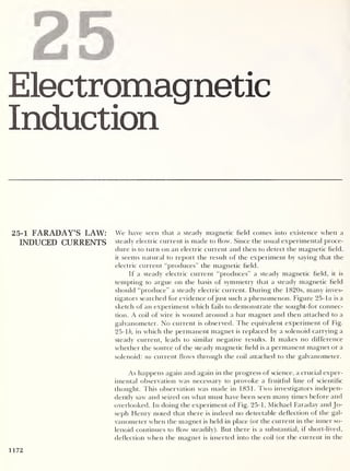
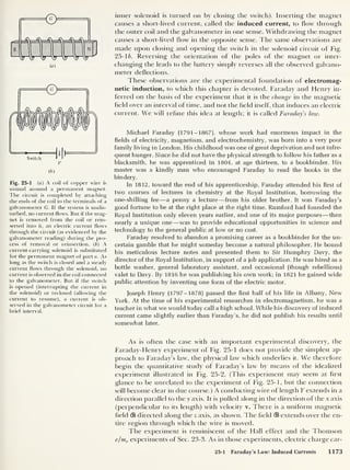
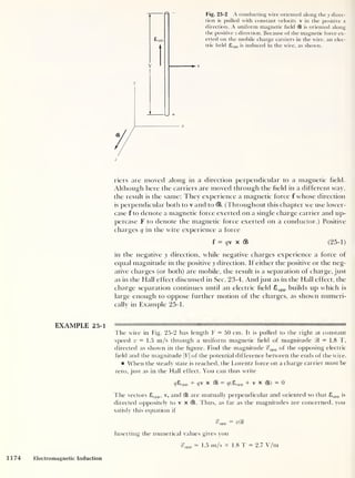
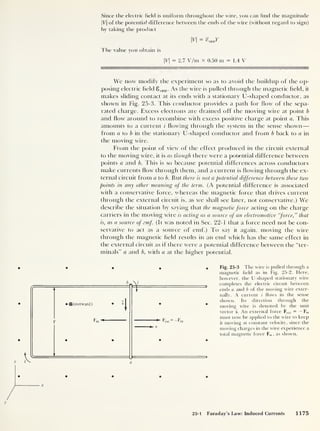
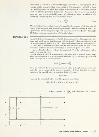
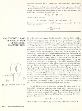
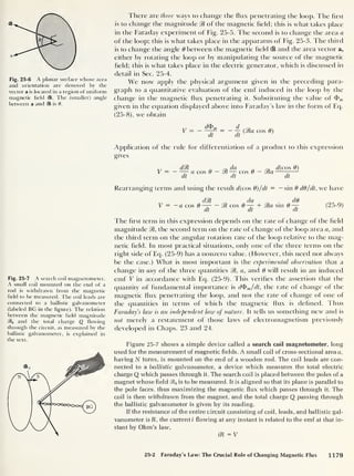
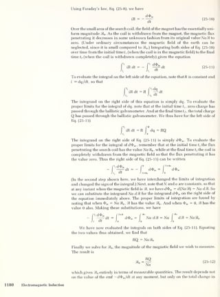
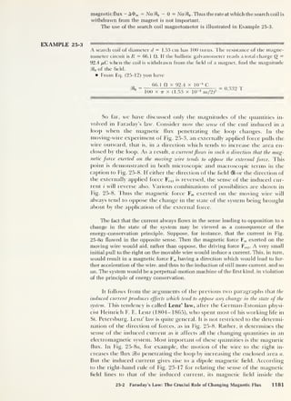
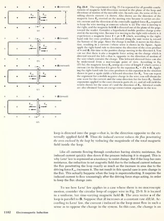
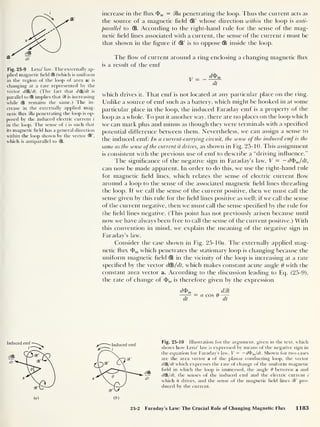
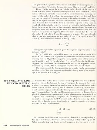
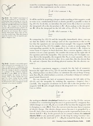
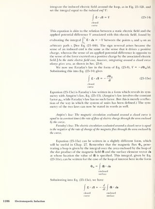
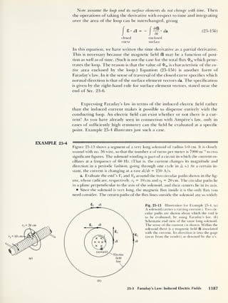
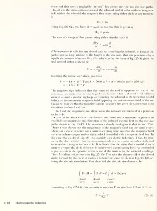
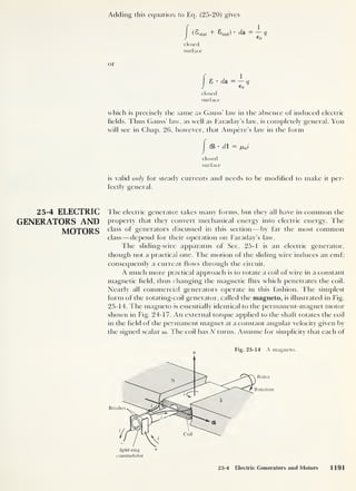
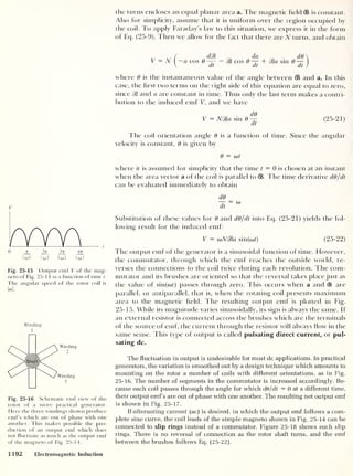
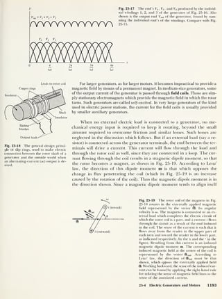
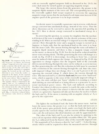
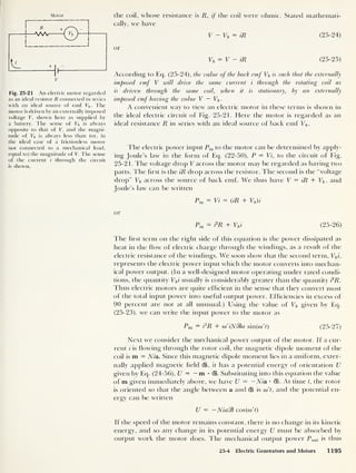
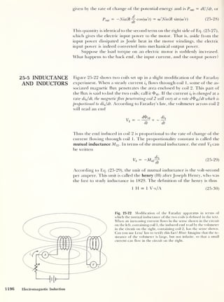
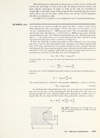
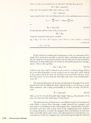
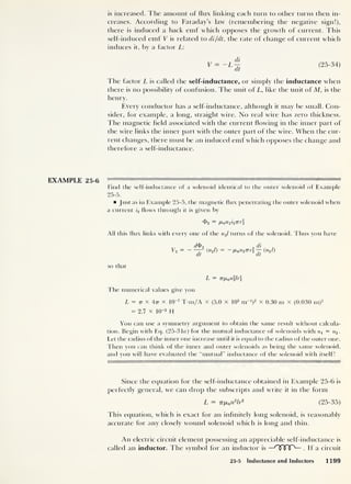
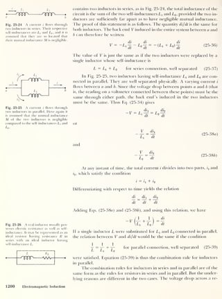
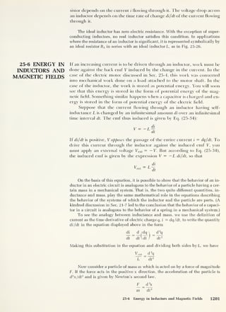
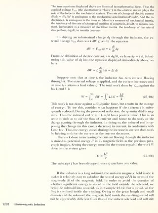
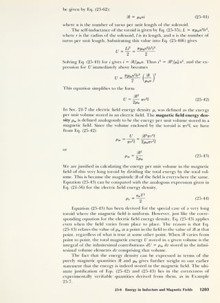
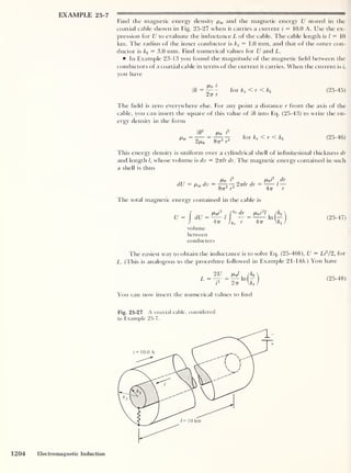
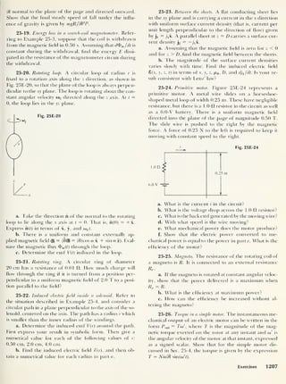
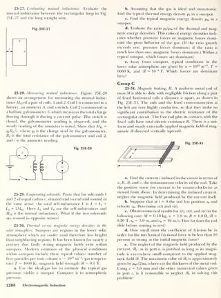
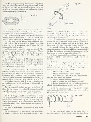
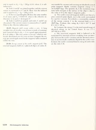
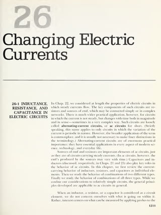
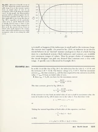
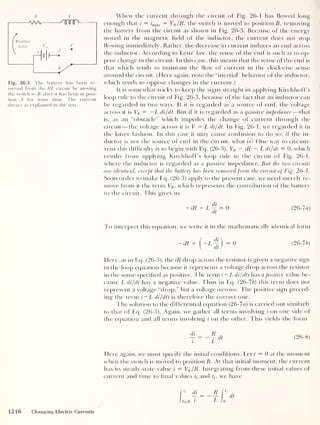
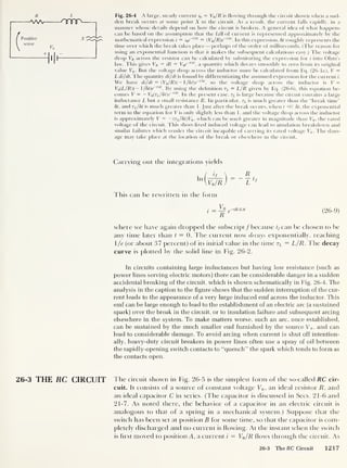
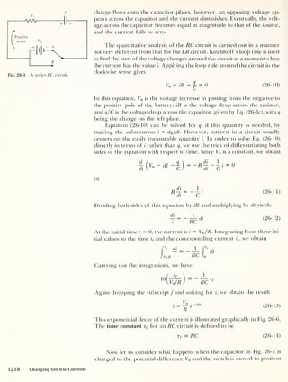
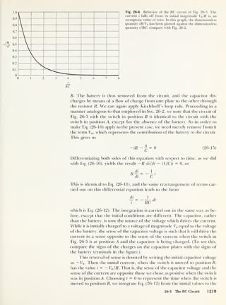
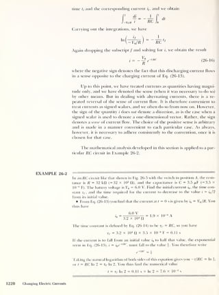
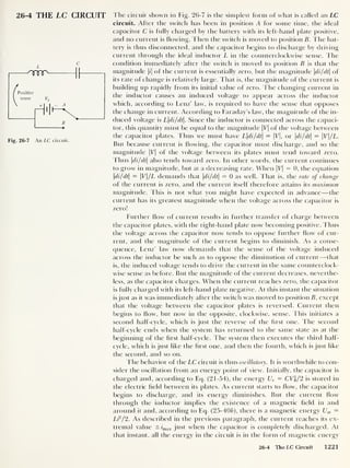
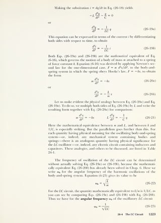
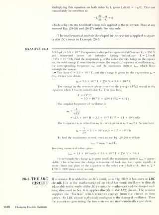
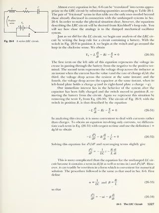
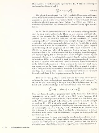
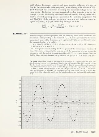
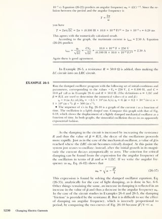
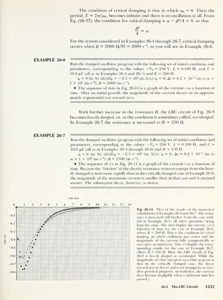
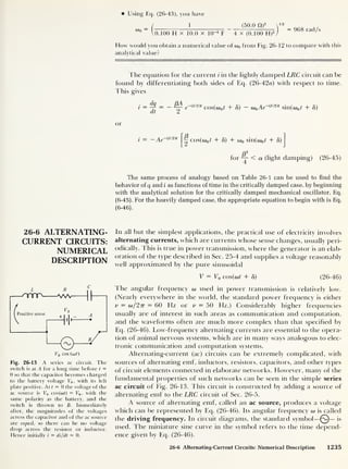
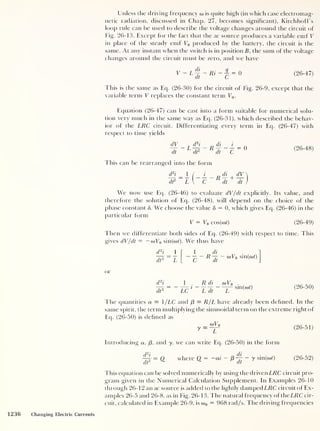
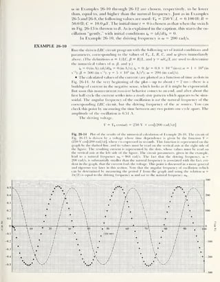
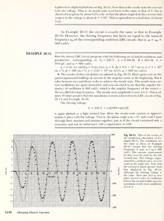
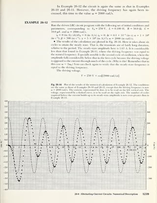
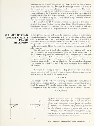
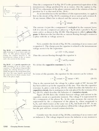
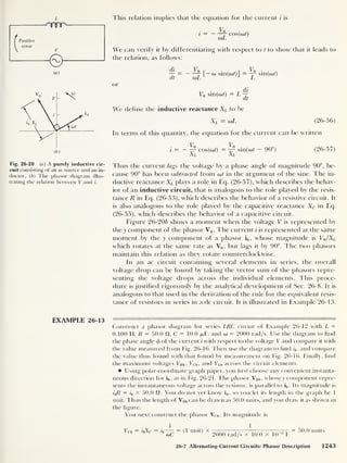
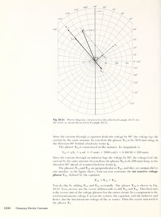
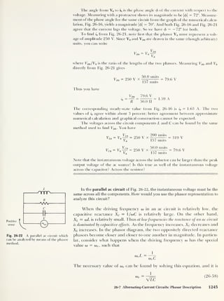
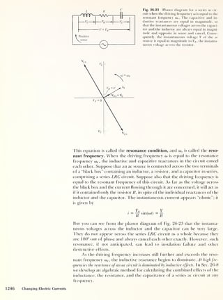
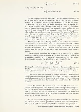
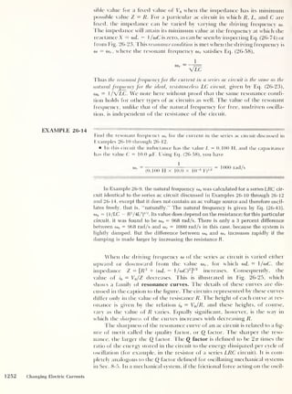
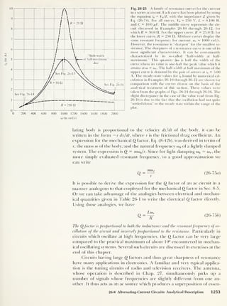
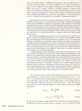
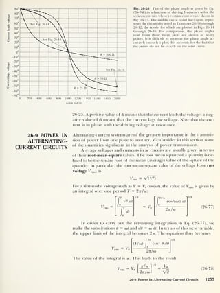
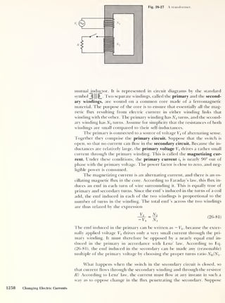
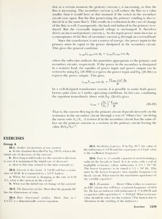
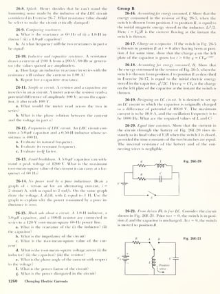
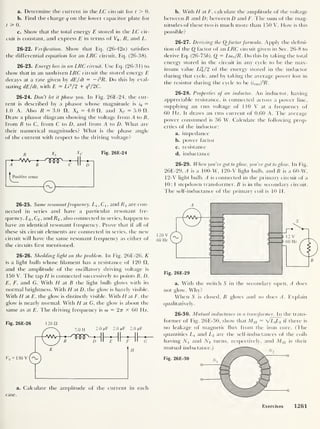
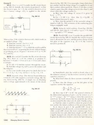
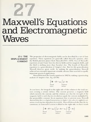
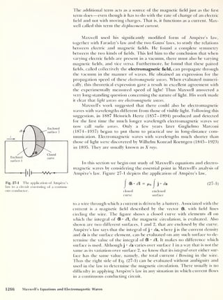
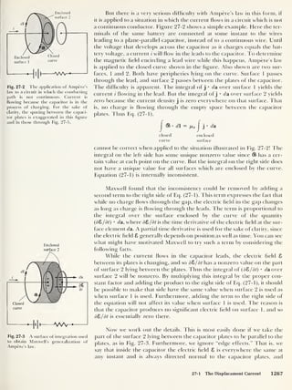
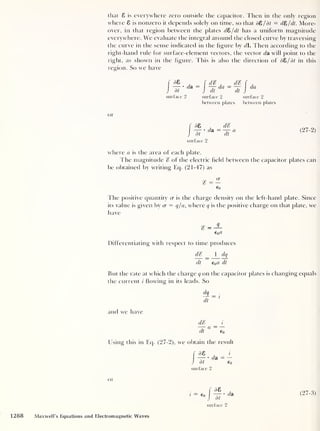
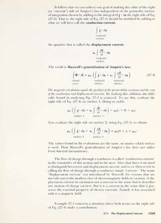
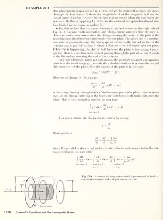
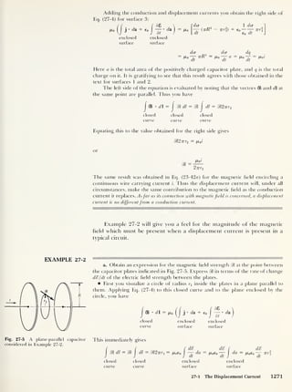
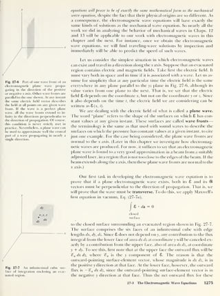
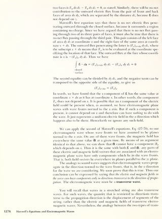
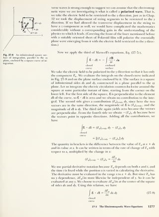
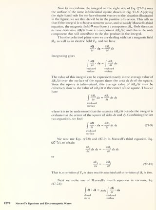
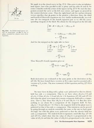
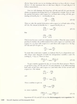
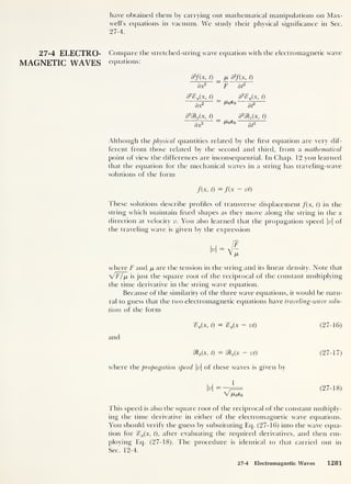
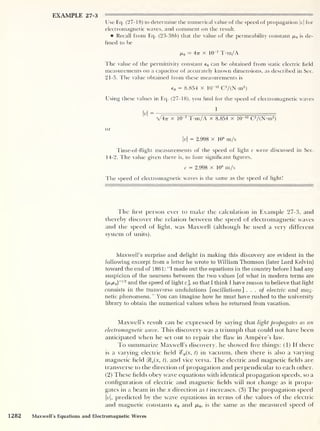
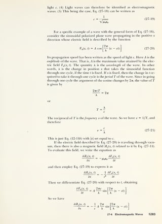
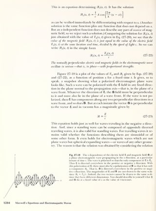
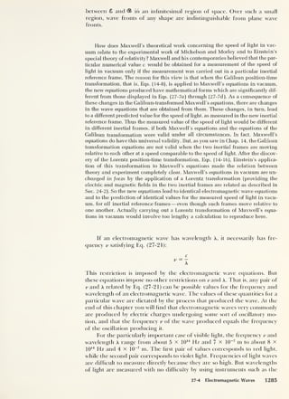
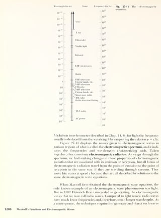
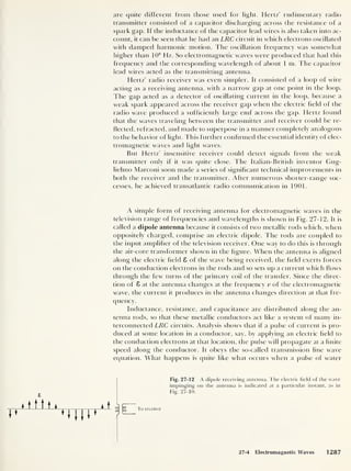
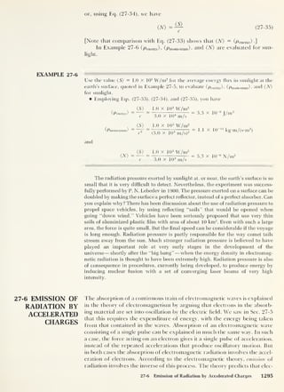
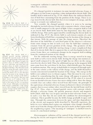
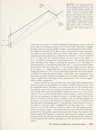
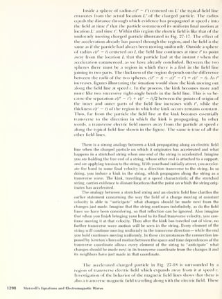
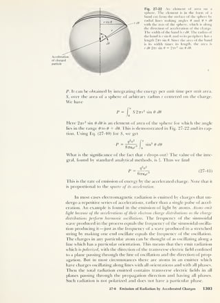
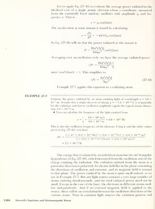
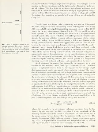
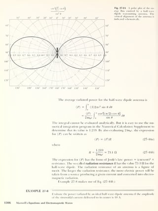
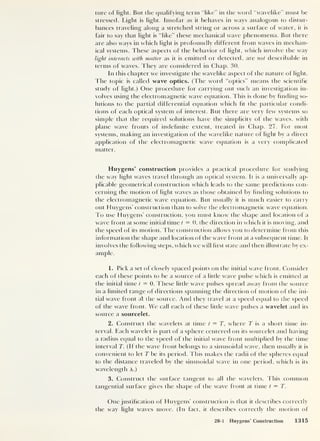
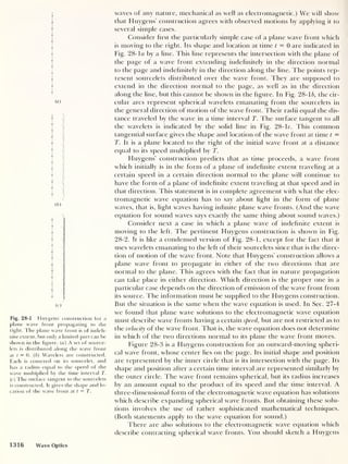
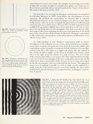
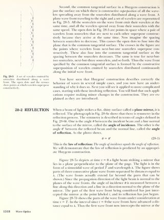
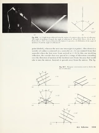
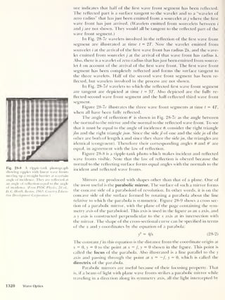
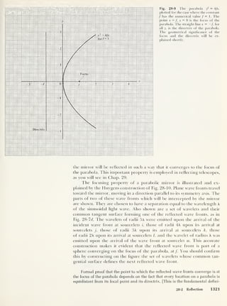
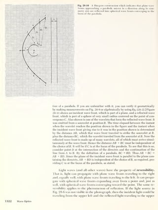
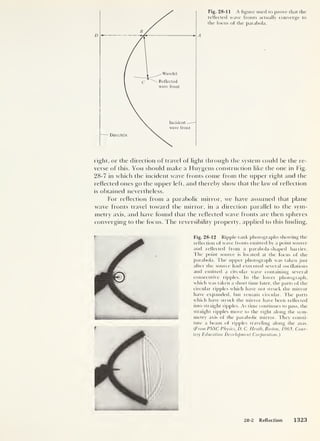
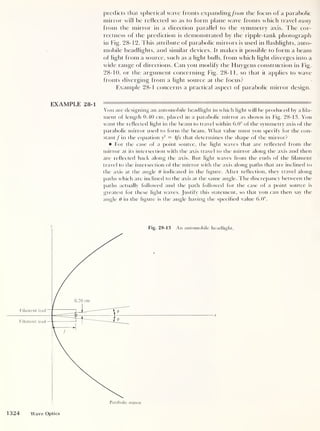
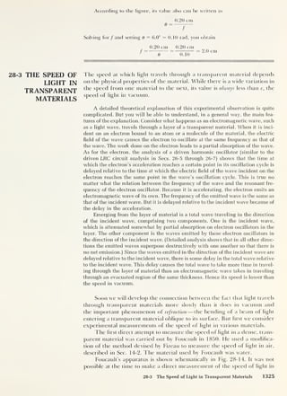
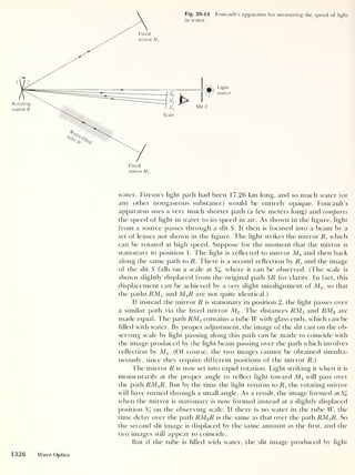
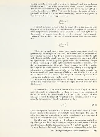
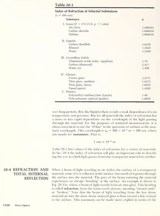
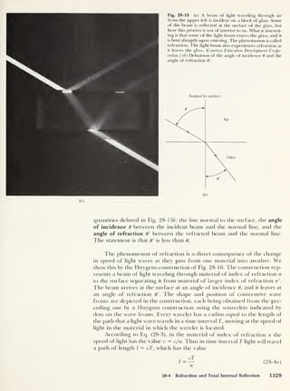
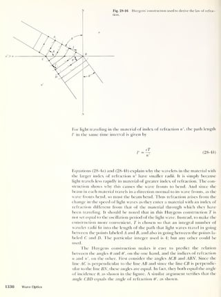
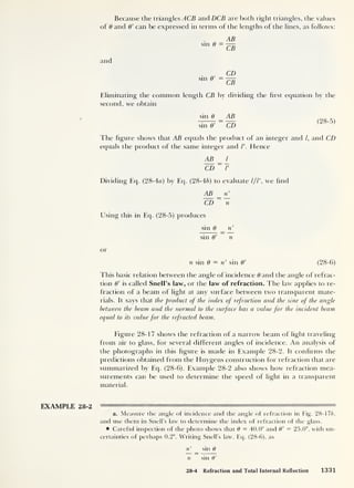
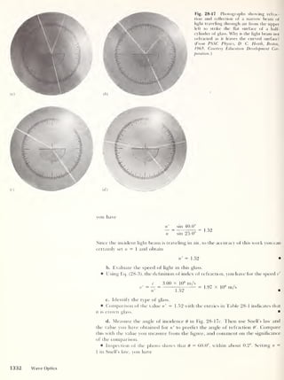
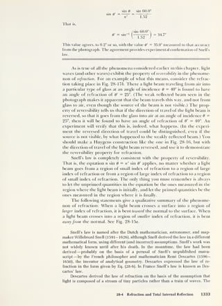
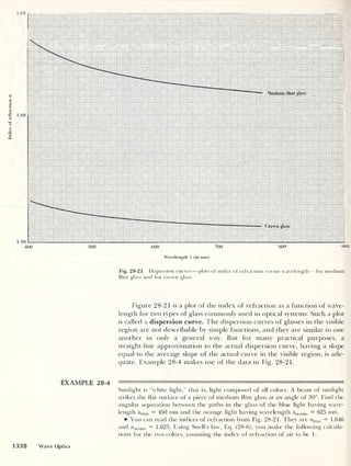
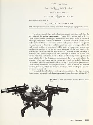
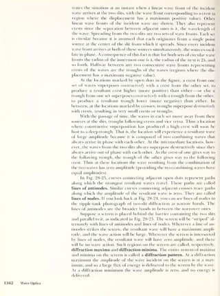
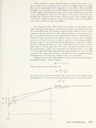
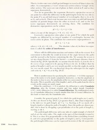
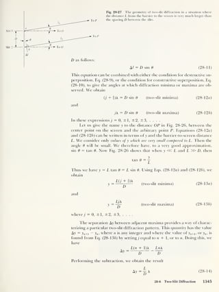
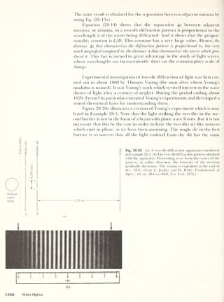
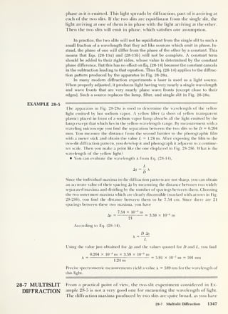
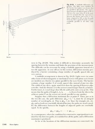
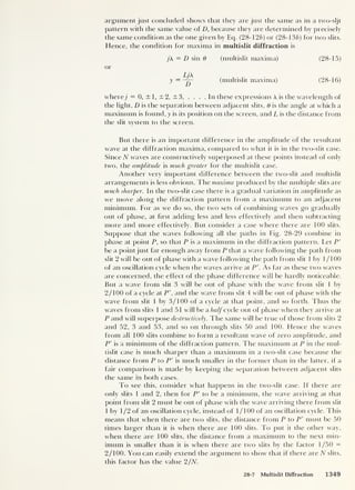
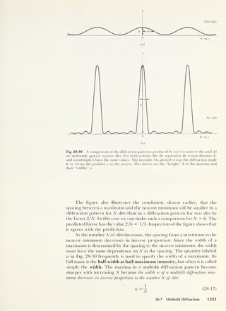
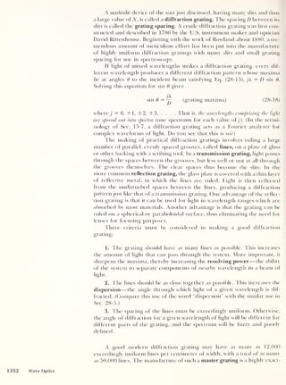
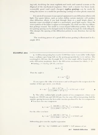
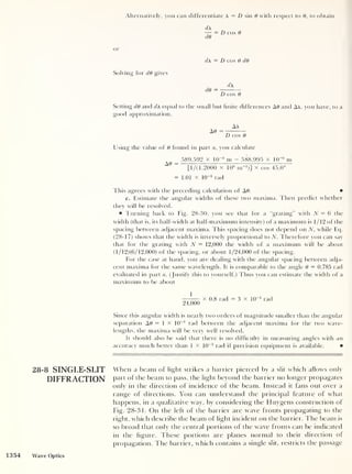
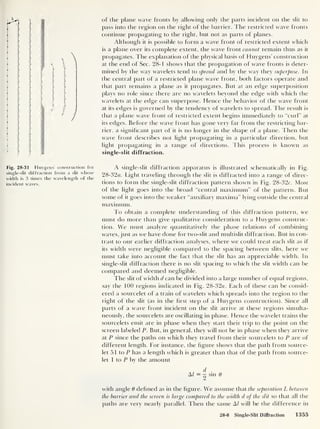
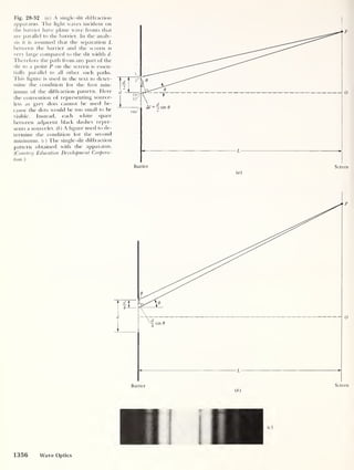
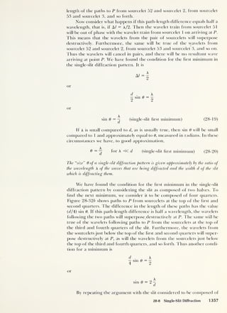
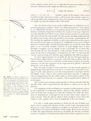
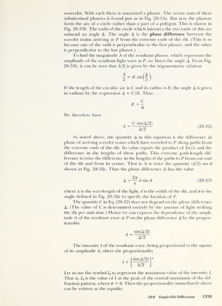
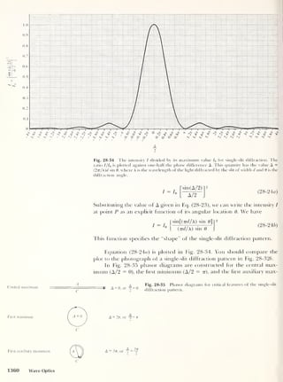
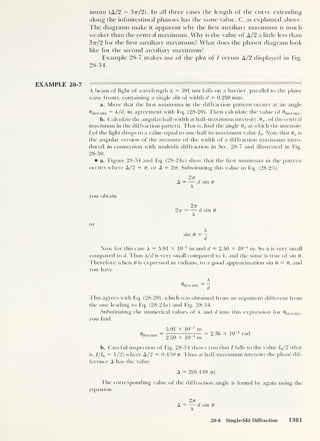
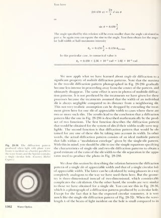
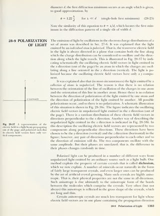
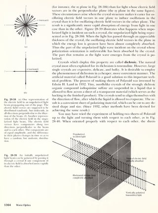
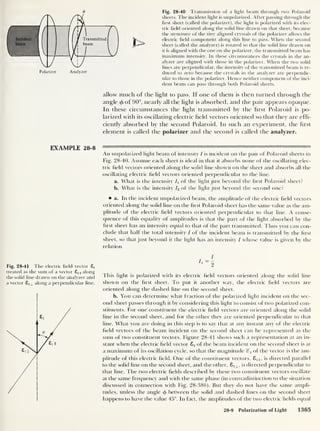
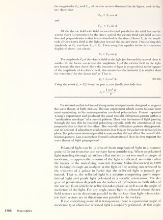
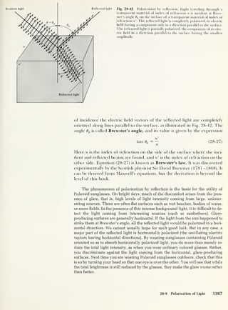
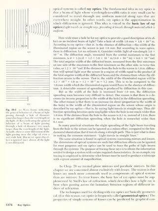
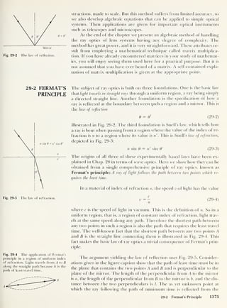
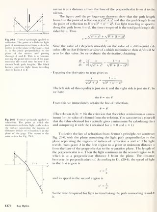
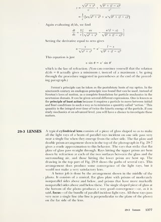
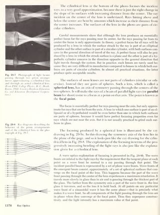
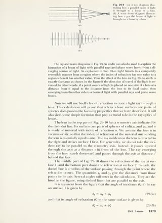
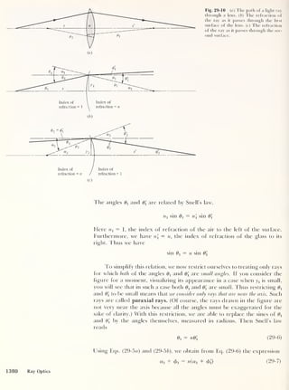
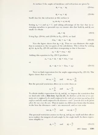
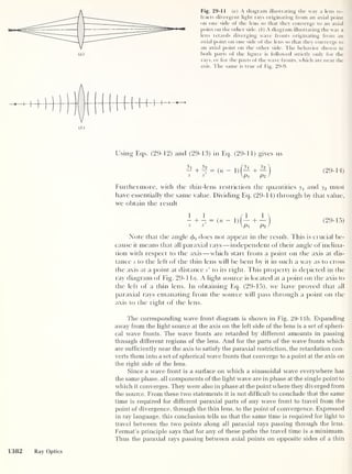
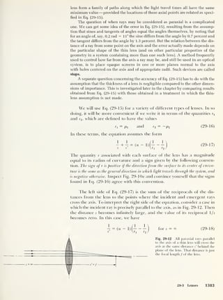
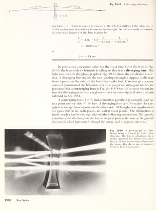
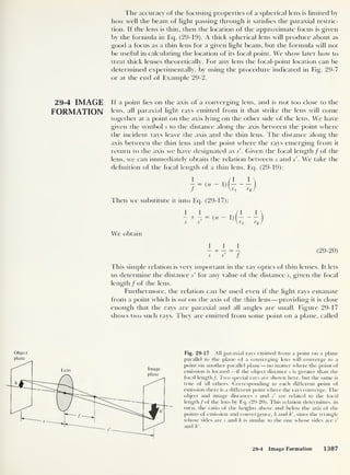
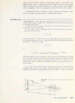
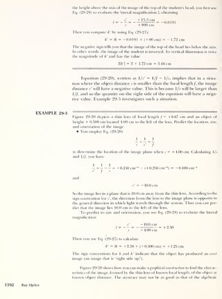
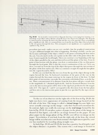
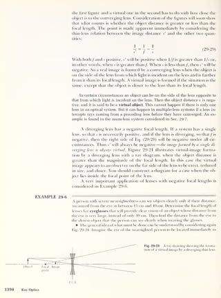
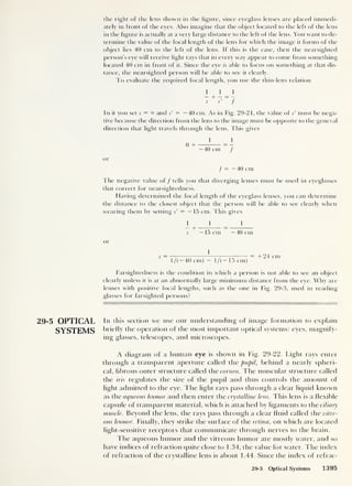
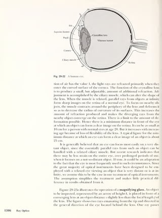
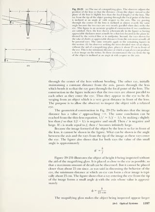
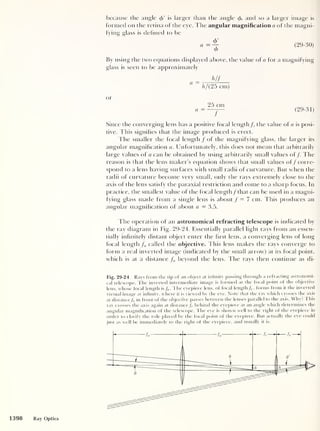
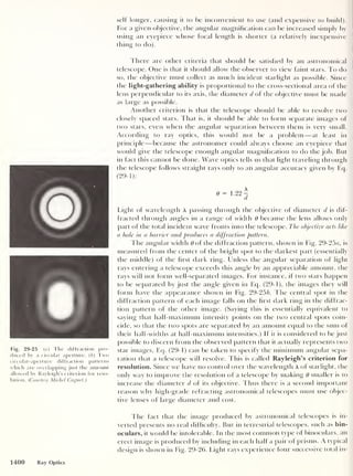
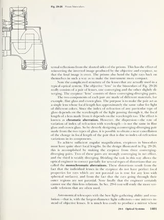
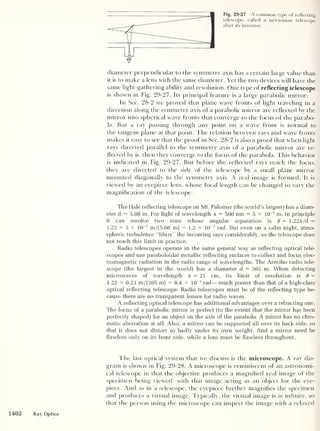
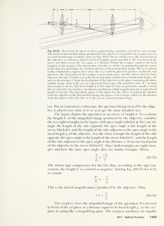
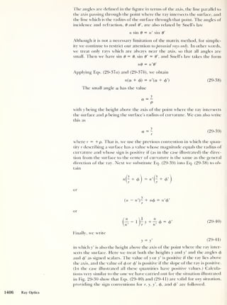
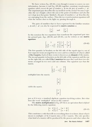
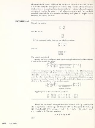
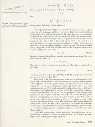
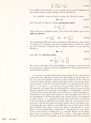
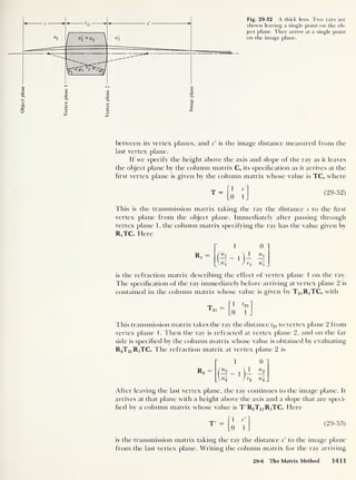
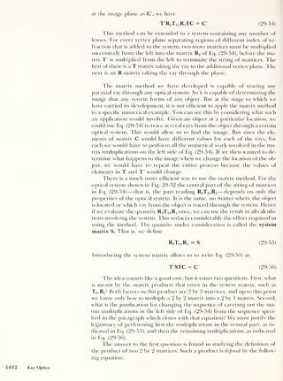
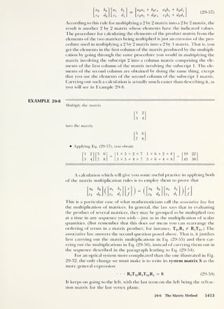
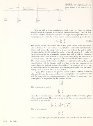
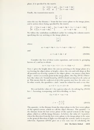
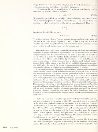
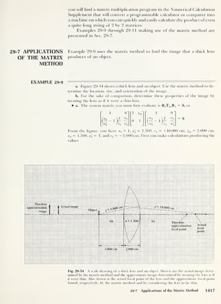
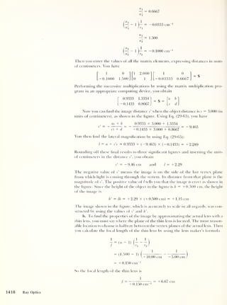
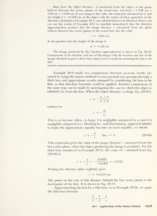
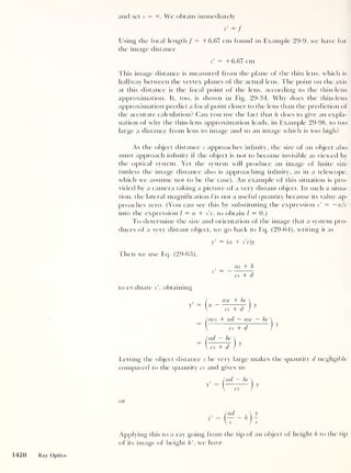
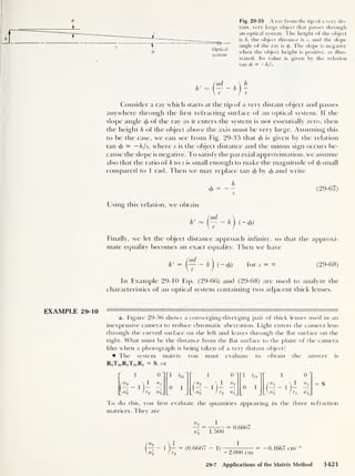
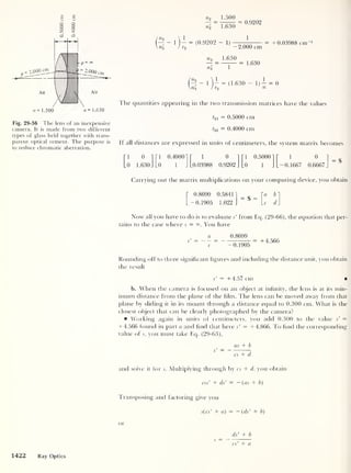
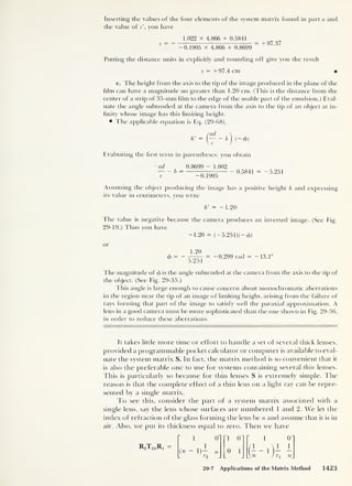
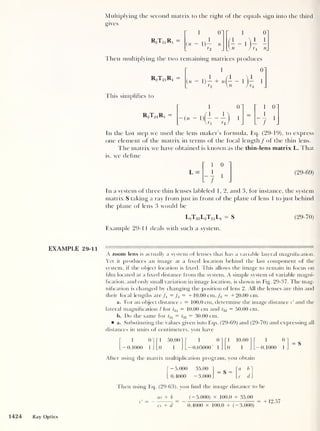
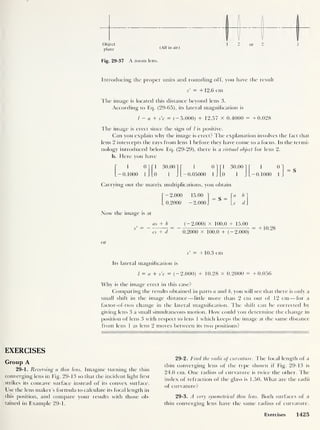
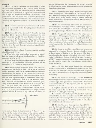
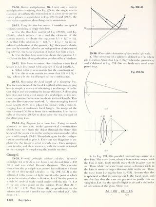

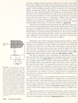
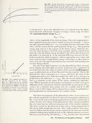
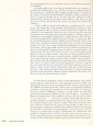
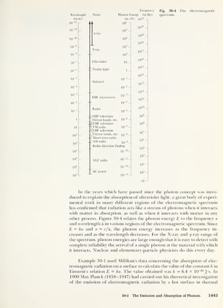
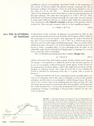
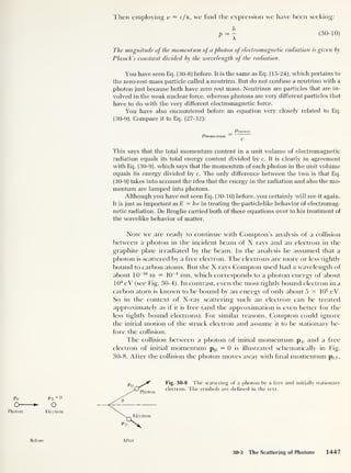
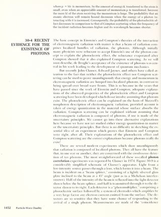
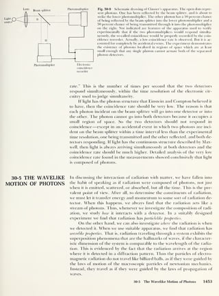
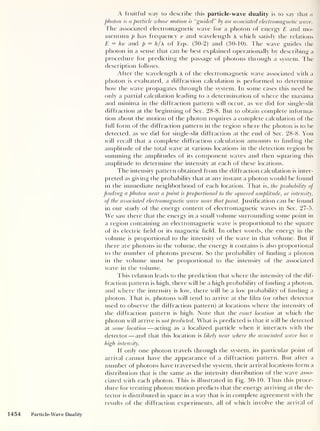
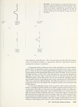
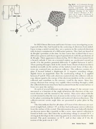
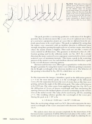
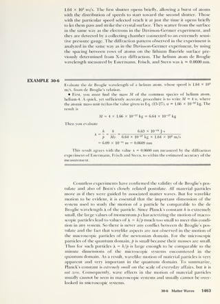
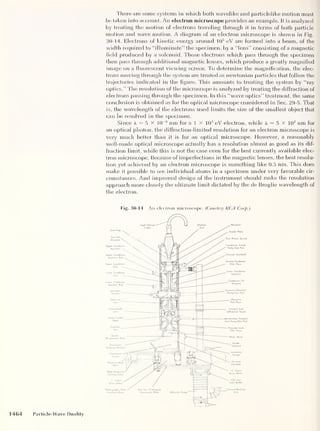
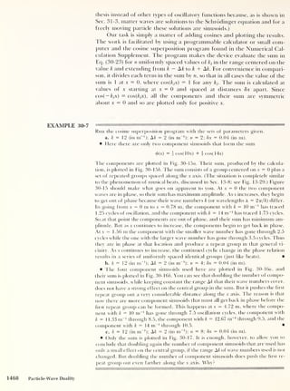
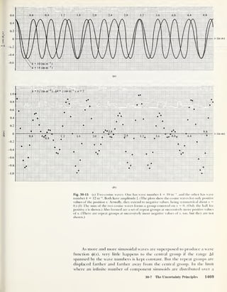
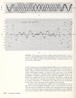
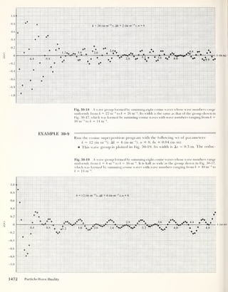
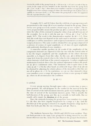
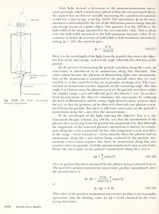
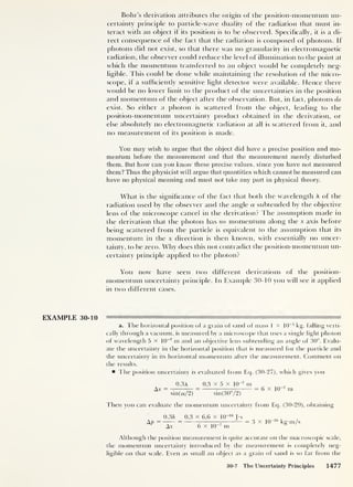
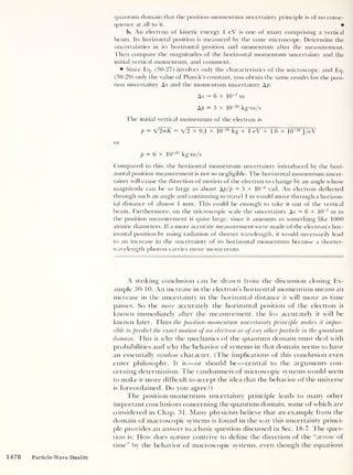
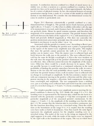
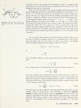
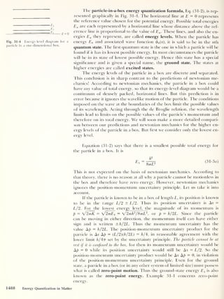
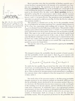
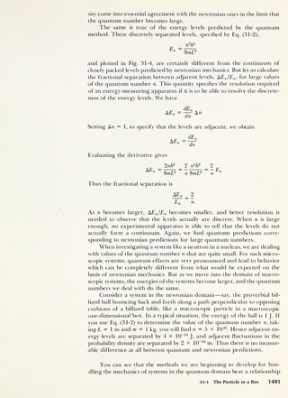
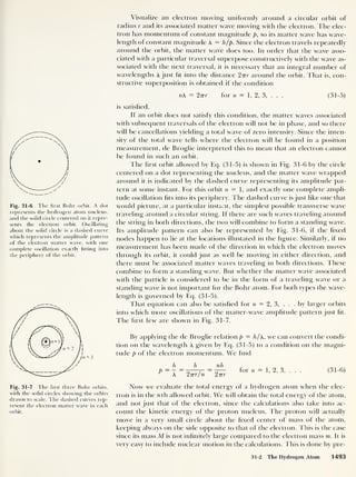
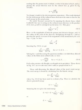
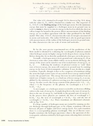
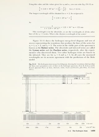
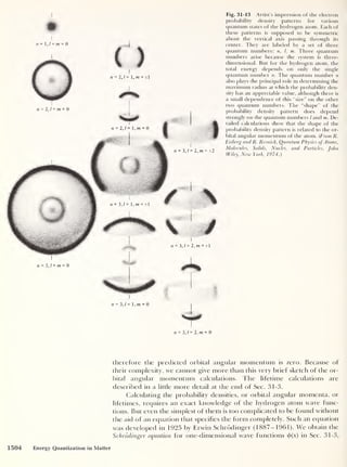
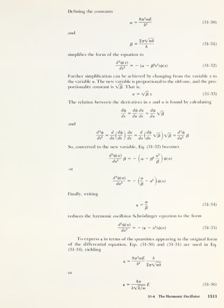
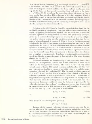
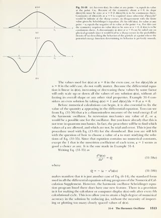

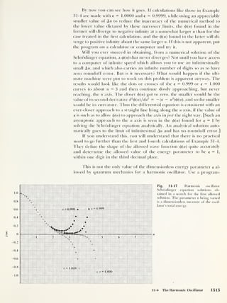
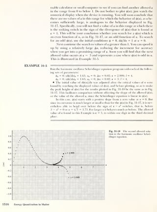
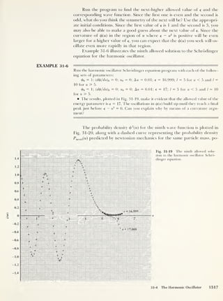
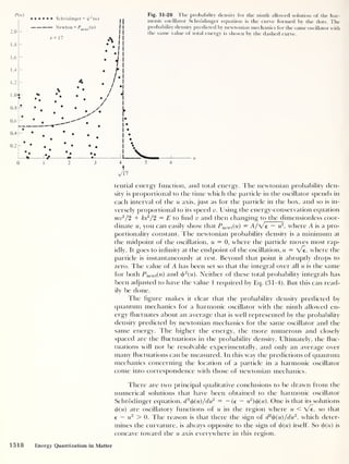
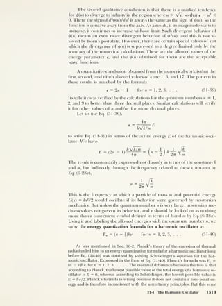
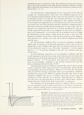
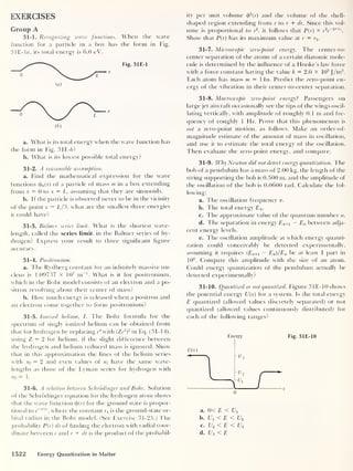

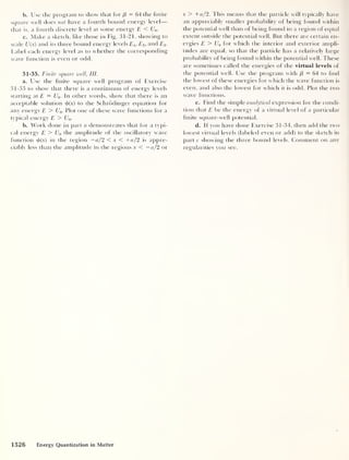


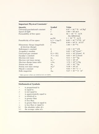
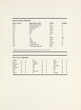


![谷歌留痕技术 [ 𝙩𝙤𝙥 𝟮𝟯𝟯. 𝙘 𝙤𝙢 ]](https://cdn.slidesharecdn.com/ss_thumbnails/top233-260130174328-3833018c-thumbnail.jpg?width=640&height=640&fit=bounds)


