Downloaded 35 times
![1 INTRODUCTION
1 Introduction
1.1 Intended audience
These lecture notes outline a single semester course intended for upper division
undergraduates.
1.2 Major sources
The textbooks which I have consulted most frequently whilst developing course
material are:
Classical electricity and magnetism: W.K.H. Panofsky, and M. Phillips, 2nd edition
(Addison-Wesley, Reading MA, 1962).
The Feynman lectures on physics: R.P. Feynman, R.B. Leighton, and M. Sands, Vol.
II (Addison-Wesley, Reading MA, 1964).
Special relativity: W. Rindler (Oliver & Boyd, Edinburgh & London UK, 1966).
Electromagnetic fields and waves: P. Lorrain, and D.R. Corson, 3rd edition (W.H. Free-
man & Co., San Francisco CA, 1970).
Electromagnetism: I.S. Grant, and W.R. Phillips (John Wiley & Sons, Chichester
UK, 1975).
Foundations of electromagnetic theory: J.R. Reitz, F.J. Milford, and R.W. Christy,
3rd edition (Addison-Wesley, Reading MA, 1980).
The classical theory of fields: E.M. Lifshitz, and L.D. Landau, 4th edition [Butterworth-
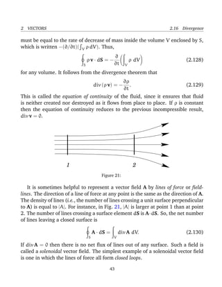
Heinemann, Oxford UK, 1980].
Introduction to electrodynamics: D.J. Griffiths, 2nd edition (Prentice Hall, Engle-
wood Cliffs NJ, 1989).
7](https://image.slidesharecdn.com/fitzpatrick-140618223522-phpapp01/85/Fitzpatrick-r-classical-electromagnetism-7-320.jpg)
![1 INTRODUCTION 1.5 Acknowledgements
1.5 Acknowledgements
My thanks to Prof. Wang-Jung Yoon [Chonnam National University, Republic of
Korea (South)] for pointing out many typographical errors appearing in earlier
editions of this work.
10](https://image.slidesharecdn.com/fitzpatrick-140618223522-phpapp01/85/Fitzpatrick-r-classical-electromagnetism-10-320.jpg)
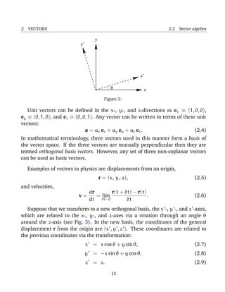
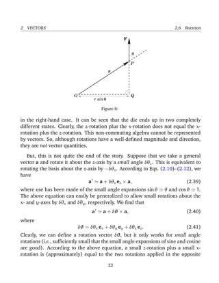
![2 VECTORS 2.3 Vector areas
We do not need to change our notation for the displacement in the new basis.
It is still denoted r. The reason for this is that the magnitude and direction of r
are independent of the choice of basis vectors. The coordinates of r do depend on
the choice of basis vectors. However, they must depend in a very specific manner
[i.e., Eqs. (2.7)–(2.9)] which preserves the magnitude and direction of r.
Since any vector can be represented as a displacement from an origin (this is
just a special case of a directed line element), it follows that the components of
a general vector a must transform in an analogous manner to Eqs. (2.7)–(2.9).
Thus,
ax = ax cos θ + ay sin θ, (2.10)
ay = −ax sin θ + ay cos θ, (2.11)
az = az, (2.12)
with similar transformation rules for rotation about the y- and z-axes. In the co-
ordinate approach, Eqs. (2.10)–(2.12) constitute the definition of a vector. The
three quantities (ax, ay, az) are the components of a vector provided that they
transform under rotation like Eqs. (2.10)–(2.12). Conversely, (ax, ay, az) cannot
be the components of a vector if they do not transform like Eqs. (2.10)–(2.12).
Scalar quantities are invariant under transformation. Thus, the individual com-
ponents of a vector (ax, say) are real numbers, but they are not scalars. Displace-
ment vectors, and all vectors derived from displacements, automatically satisfy
Eqs. (2.10)–(2.12). There are, however, other physical quantities which have
both magnitude and direction, but which are not obviously related to displace-
ments. We need to check carefully to see whether these quantities are vectors.
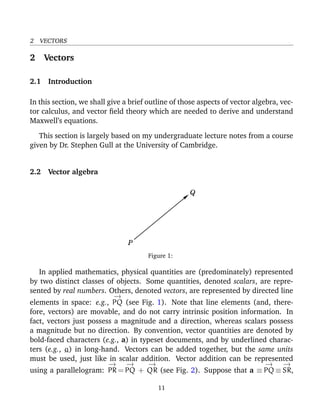
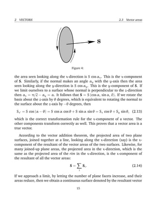
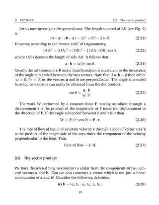
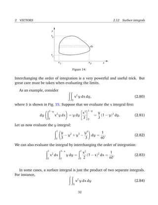
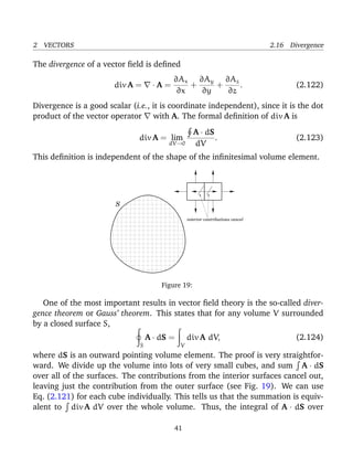
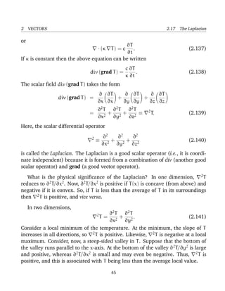
2.3 Vector areas
Suppose that we have planar surface of scalar area S. We can define a vector
area S whose magnitude is S, and whose direction is perpendicular to the plane,
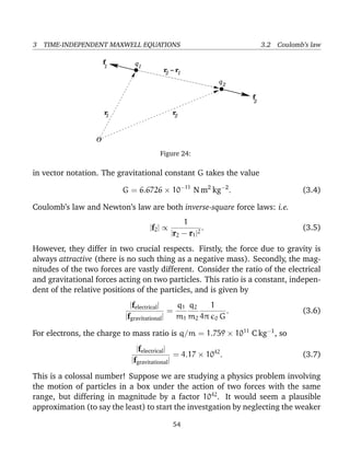
in the sense determined by the right-hand grip rule on the rim (see Fig. 4). This
quantity clearly possesses both magnitude and direction. But is it a true vector?
We know that if the normal to the surface makes an angle αx with the x-axis then
14](https://image.slidesharecdn.com/fitzpatrick-140618223522-phpapp01/85/Fitzpatrick-r-classical-electromagnetism-14-320.jpg)
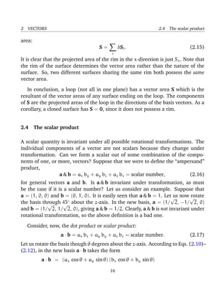
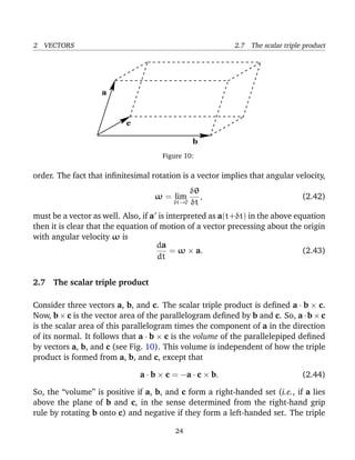
![2 VECTORS 2.9 Vector calculus
Let us try to prove the first of the above theorems. The left-hand side and
the right-hand side are both proper vectors, so if we can prove this result in
one particular coordinate system then it must be true in general. Let us take
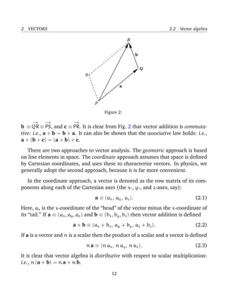
convenient axes such that the x-axis lies along b, and c lies in the x-y plane. It
follows that b = (bx, 0, 0), c = (cx, cy, 0), and a = (ax, ay, az). The vector b × c
is directed along the z-axis: b × c = (0, 0, bx cy). It follows that a × (b × c) lies
in the x-y plane: a × (b × c) = (ay bx cy, −ax bx cy, 0). This is the left-hand side
of Eq. (2.51) in our convenient axes. To evaluate the right-hand side, we need
a · c = ax cx + ay cy and a · b = ax bx. It follows that the right-hand side is
RHS = ( [ax cx + ay cy] bx, 0, 0) − (ax bx cx, ax bx cy, 0)
= (ay cy bx, −ax bx cy, 0) = LHS, (2.53)
which proves the theorem.
2.9 Vector calculus
Suppose that vector a varies with time, so that a = a(t). The time derivative of
the vector is defined
da
dt
= lim
δt→0
a(t + δt) − a(t)
δt
. (2.54)
When written out in component form this becomes
da
dt
=
dax
dt
,
day
dt
,
daz
dt
. (2.55)
Suppose that a is, in fact, the product of a scalar φ(t) and another vector b(t).
What now is the time derivative of a? We have
dax
dt
=
d
dt
(φ bx) =
dφ
dt
bx + φ
dbx
dt
, (2.56)
which implies that
da
dt
=
dφ
dt
b + φ
db
dt
. (2.57)
26](https://image.slidesharecdn.com/fitzpatrick-140618223522-phpapp01/85/Fitzpatrick-r-classical-electromagnetism-26-320.jpg)
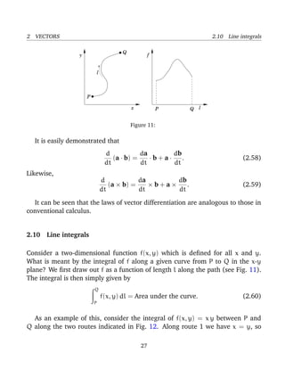
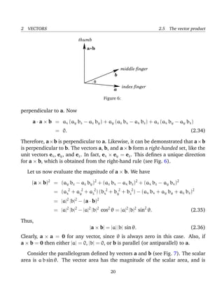
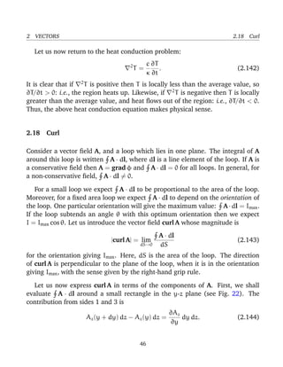
![2 VECTORS 2.10 Line integrals
x
y
Q = (1, 1)
P = (0, 0)
2
2
1
Figure 12:
dl =
√
2 dx. Thus,
Q
P
x y dl =
1
0
x2
√
2 dx =
√
2
3
. (2.61)
The integration along route 2 gives
Q
P
x y dl =
1
0
x y dx
y=0
+
1
0
x y dy
x=1
= 0 +
1
0
y dy =
1
2
. (2.62)
Note that the integral depends on the route taken between the initial and final
points.
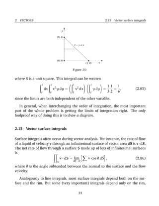
The most common type of line integral is that where the contributions from
dx and dy are evaluated separately, rather that through the path length dl:
Q
P
[f(x, y) dx + g(x, y) dy] . (2.63)
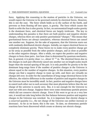
As an example of this, consider the integral
Q
P
y3
dx + x dy (2.64)
along the two routes indicated in Fig. 13. Along route 1 we have x = y + 1 and
28](https://image.slidesharecdn.com/fitzpatrick-140618223522-phpapp01/85/Fitzpatrick-r-classical-electromagnetism-28-320.jpg)
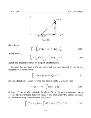
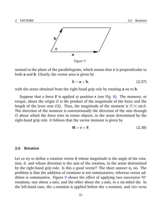
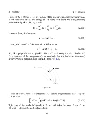
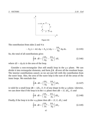
![2 VECTORS 2.15 Gradient
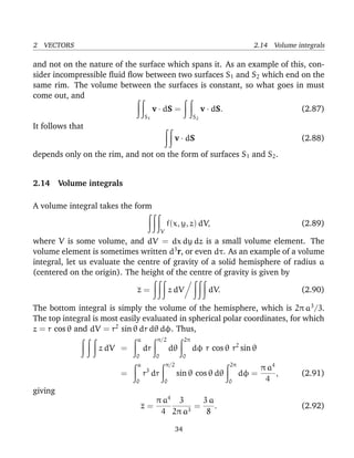
2.15 Gradient
A one-dimensional function f(x) has a gradient df/dx which is defined as the
slope of the tangent to the curve at x. We wish to extend this idea to cover scalar
fields in two and three dimensions.
x
y
P
θ
contours of h(x, y)
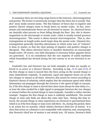
Figure 16:
Consider a two-dimensional scalar field h(x, y), which is (say) the height of
a hill. Let dl = (dx, dy) be an element of horizontal distance. Consider dh/dl,
where dh is the change in height after moving an infinitesimal distance dl. This
quantity is somewhat like the one-dimensional gradient, except that dh depends
on the direction of dl, as well as its magnitude. In the immediate vicinity of some
point P, the slope reduces to an inclined plane (see Fig. 16). The largest value of
dh/dl is straight up the slope. For any other direction
dh
dl
=
dh
dl max
cos θ. (2.93)
Let us define a two-dimensional vector, grad h, called the gradient of h, whose
magnitude is (dh/dl)max, and whose direction is the direction up the steepest
slope. Because of the cos θ property, the component of grad h in any direction
equals dh/dl for that direction. [The argument, here, is analogous to that used
for vector areas in Sect. 2.3. See, in particular, Eq. (2.13). ]
The component of dh/dl in the x-direction can be obtained by plotting out the
profile of h at constant y, and then finding the slope of the tangent to the curve
at given x. This quantity is known as the partial derivative of h with respect to x
35](https://image.slidesharecdn.com/fitzpatrick-140618223522-phpapp01/85/Fitzpatrick-r-classical-electromagnetism-35-320.jpg)
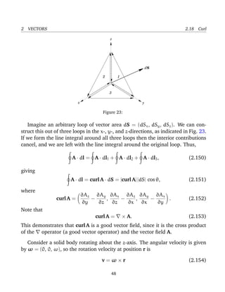
![2 VECTORS 2.18 Curl
[see Eq. (2.43) ]. Let us evaluate curl v on the axis of rotation. The x-component
is proportional to the integral v · dl around a loop in the y-z plane. This is
plainly zero. Likewise, the y-component is also zero. The z-component is v ·
dl/dS around some loop in the x-y plane. Consider a circular loop. We have
v · dl = 2π r ω r with dS = π r2
. Here, r is the radial distance from the rotation
axis. It follows that (curl v)z = 2 ω, which is independent of r. So, on the axis,
curl v = (0 , 0 , 2 ω). Off the axis, at position r0, we can write
v = ω × (r − r0) + ω × r0. (2.155)
The first part has the same curl as the velocity field on the axis, and the second
part has zero curl, since it is constant. Thus, curl v = (0, 0, 2 ω) everywhere in
the body. This allows us to form a physical picture of curl A. If we imagine A as
the velocity field of some fluid, then curl A at any given point is equal to twice
the local angular rotation velocity: i.e., 2 ω. Hence, a vector field with curl A = 0
everywhere is said to be irrotational.
Another important result of vector field theory is the curl theorem or Stokes’
theorem,
C
A · dl =
S
curl A · dS, (2.156)
for some (non-planar) surface S bounded by a rim C. This theorem can easily be
proved by splitting the loop up into many small rectangular loops, and forming
the integral around all of the resultant loops. All of the contributions from the
interior loops cancel, leaving just the contribution from the outer rim. Making
use of Eq. (2.151) for each of the small loops, we can see that the contribution
from all of the loops is also equal to the integral of curl A · dS across the whole
surface. This proves the theorem.
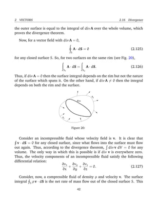
One immediate consequence of Stokes’ theorem is that curl A is “incompress-
ible.” Consider two surfaces, S1 and S2, which share the same rim. It is clear
from Stokes’ theorem that curl A · dS is the same for both surfaces. Thus, it
follows that curl A · dS = 0 for any closed surface. However, we have from the
divergence theorem that curl A · dS = div (curl A) dV = 0 for any volume.
Hence,
div (curl A) ≡ 0. (2.157)
49](https://image.slidesharecdn.com/fitzpatrick-140618223522-phpapp01/85/Fitzpatrick-r-classical-electromagnetism-49-320.jpg)
![3 TIME-INDEPENDENT MAXWELL EQUATIONS 3.3 The electric scalar potential
3.3 The electric scalar potential
Suppose that r = (x, y, z) and r = (x , y , z ) in Cartesian coordinates. The x
component of (r − r )/|r − r |3
is written
x − x
[(x − x )2 + (y − y )2 + (z − z )2]3/2
. (3.13)
However, it is easily demonstrated that
x − x
[(x − x )2 + (y − y )2 + (z − z )2]3/2
= (3.14)
−
∂
∂x
1
[(x − x )2 + (y − y )2 + (z − z )2] 1/2
.
Since there is nothing special about the x-axis, we can write
r − r
|r − r |3
= −
1
|r − r |
, (3.15)
where ≡ (∂/∂x, ∂/∂y, ∂/∂z) is a differential operator which involves the com-
ponents of r but not those of r . It follows from Eq. (3.12) that
E = − φ, (3.16)
where
φ(r) =
1
4π 0
ρ(r )
|r − r |
d3
r . (3.17)
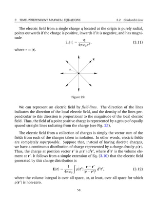
Thus, the electric field generated by a collection of fixed charges can be written as
the gradient of a scalar potential, and this potential can be expressed as a simple
volume integral involving the charge distribution.
The scalar potential generated by a charge q located at the origin is
φ(r) =
q
4π 0 r
. (3.18)
According to Eq. (3.10), the scalar potential generated by a set of N discrete
charges qi, located at ri, is
φ(r) =
N
i=1
φi(r), (3.19)
59](https://image.slidesharecdn.com/fitzpatrick-140618223522-phpapp01/85/Fitzpatrick-r-classical-electromagnetism-59-320.jpg)
![3 TIME-INDEPENDENT MAXWELL EQUATIONS 3.3 The electric scalar potential
where
φi(r) =
qi
4π 0 |r − ri|
. (3.20)
Thus, the scalar potential is just the sum of the potentials generated by each of
the charges taken in isolation.
Suppose that a particle of charge q is taken along some path from point P to
point Q. The net work done on the particle by electrical forces is
W =
Q
P
f · dl, (3.21)
where f is the electrical force, and dl is a line element along the path. Making
use of Eqs. (3.9) and (3.16), we obtain
W = q
Q
P
E · dl = −q
Q
P
φ · dl = −q [ φ(Q) − φ(P) ] . (3.22)
Thus, the work done on the particle is simply minus its charge times the differ-
ence in electric potential between the end point and the beginning point. This
quantity is clearly independent of the path taken between P and Q. So, an elec-
tric field generated by stationary charges is an example of a conservative field. In
fact, this result follows immediately from vector field theory once we are told, in
Eq. (3.16), that the electric field is the gradient of a scalar potential. The work
done on the particle when it is taken around a closed loop is zero, so
C
E · dl = 0 (3.23)
for any closed loop C. This implies from Stokes’ theorem that
× E = 0 (3.24)
for any electric field generated by stationary charges. Equation (3.24) also fol-
lows directly from Eq. (3.16), since × φ = 0 for any scalar potential φ.
The SI unit of electric potential is the volt, which is equivalent to a joule per
coulomb. Thus, according to Eq. (3.22), the electrical work done on a particle
when it is taken between two points is the product of its charge and the voltage
difference between the points.
60](https://image.slidesharecdn.com/fitzpatrick-140618223522-phpapp01/85/Fitzpatrick-r-classical-electromagnetism-60-320.jpg)
![3 TIME-INDEPENDENT MAXWELL EQUATIONS 3.4 Gauss’ law
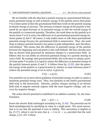
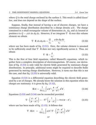
for a spherical volume V centered on the origin. These two facts imply that
· E =
q
0
δ(r), (3.48)
where use has been made of Eq. (3.43).
At this stage, vector field theory has yet to show its worth.. After all, we have
just spent an inordinately long time proving something using vector field theory
which we previously proved in one line [see Eq. (3.27) ] using conventional anal-
ysis. It is time to demonstrate the power of vector field theory. Consider, again,
a charge q at the origin surrounded by a spherical surface S which is centered on
the origin. Suppose that we now displace the surface S, so that it is no longer
centered on the origin. What is the flux of the electric field out of S? This is not
a simple problem for conventional analysis, because the normal to the surface is
no longer parallel to the local electric field. However, using vector field theory
this problem is no more difficult than the previous one. We have
S
E · dS =
V
· E d3
r (3.49)
from Gauss’ theorem, plus Eq. (3.48). From these equations, it is clear that the
flux of E out of S is q/ 0 for a spherical surface displaced from the origin. How-
ever, the flux becomes zero when the displacement is sufficiently large that the
origin is no longer enclosed by the sphere. It is possible to prove this via con-
ventional analysis, but it is certainly not easy. Suppose that the surface S is not
spherical but is instead highly distorted. What now is the flux of E out of S? This
is a virtually impossible problem in conventional analysis, but it is still easy using
vector field theory. Gauss’ theorem and Eq. (3.48) tell us that the flux is q/ 0
provided that the surface contains the origin, and that the flux is zero otherwise.
This result is completely independent of the shape of S.
Consider N charges qi located at ri. A simple generalization of Eq. (3.48) gives
· E =
N
i=1
qi
0
δ(r − ri). (3.50)
Thus, Gauss’ theorem (3.49) implies that
S
E · dS =
V
· E d3
r =
Q
0
, (3.51)
66](https://image.slidesharecdn.com/fitzpatrick-140618223522-phpapp01/85/Fitzpatrick-r-classical-electromagnetism-66-320.jpg)
![3 TIME-INDEPENDENT MAXWELL EQUATIONS 3.6 Amp`ere’s experiments
as a Green’s function. The solution generated by a general source function v(r) is
simply the appropriately weighted sum of all of the Green’s function solutions:
u(r) = G(r, r ) v(r ) d3
r . (3.64)
We can easily demonstrate that this is the correct solution:
2
u(r) = 2
G(r, r ) v(r ) d3
r = δ(r − r ) v(r ) d3
r = v(r). (3.65)
Let us return to Eq. (3.59):
2
φ = −
ρ
0
. (3.66)
The Green’s function for this equation satisfies Eq. (3.63) with |G| → ∞ as |r| → 0.
It follows from Eq. (3.55) that
G(r, r ) = −
1
4π
1
|r − r |
. (3.67)
Note, from Eq. (3.20), that the Green’s function has the same form as the poten-
tial generated by a point charge. This is hardly surprising, given the definition of
a Green’s function. It follows from Eq. (3.64) and (3.67) that the general solution
to Poisson’s equation, (3.66), is written
φ(r) =
1
4π 0
ρ(r )
|r − r |
d3
r . (3.68)
In fact, we have already obtained this solution by another method [see Eq. (3.17) ].
3.6 Amp`ere’s experiments
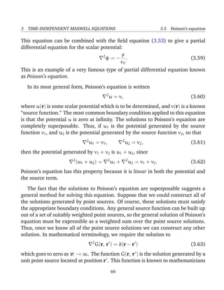
As legend has it, in 1820 the Danish physicist Hans Christian Ørsted was giving
a lecture demonstration of various electrical and magnetic effects. Suddenly,
much to his surprise, he noticed that the needle of a compass he was hold-
ing was deflected when he moved it close to a current carrying wire. Up until
70](https://image.slidesharecdn.com/fitzpatrick-140618223522-phpapp01/85/Fitzpatrick-r-classical-electromagnetism-70-320.jpg)
![3 TIME-INDEPENDENT MAXWELL EQUATIONS 3.8 Amp`ere’s law
Note that a charged particle can gain (or lose) energy from an electric field, but
not from a magnetic field. This is because the magnetic force is always perpen-
dicular to the particle’s direction of motion, and, therefore, does no work on the
particle [see Eq. (3.90) ]. Thus, in particle accelerators, magnetic fields are of-
ten used to guide particle motion (e.g., in a circle) but the actual acceleration is
performed by electric fields.
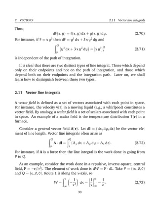
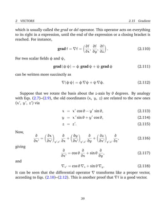
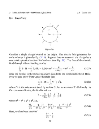
3.8 Amp`ere’s law
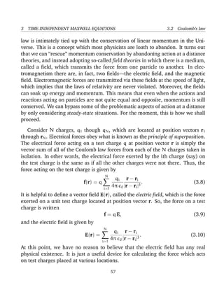
Magnetic fields, like electric fields, are completely superposable. So, if a field B1 is
generated by a current I1 flowing through some circuit, and a field B2 is generated
by a current I2 flowing through another circuit, then when the currents I1 and I2
flow through both circuits simultaneously the generated magnetic field is B1 +B2.
B
I I1 2
2
1
B
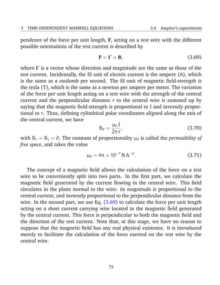
Figure 30:
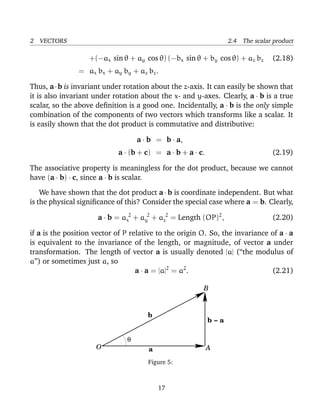
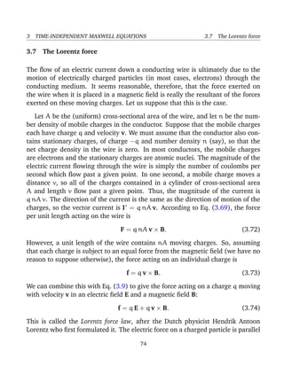
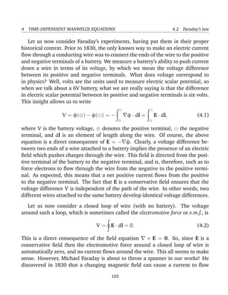
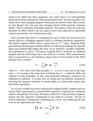
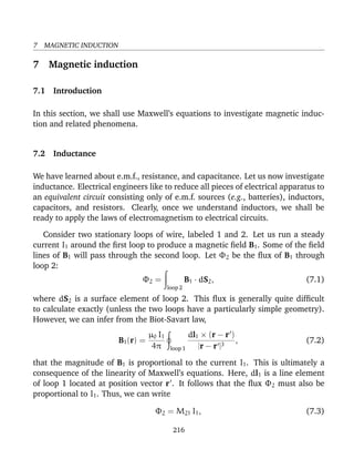
Consider two parallel wires separated by a perpendicular distance r and car-
rying electric currents I1 and I2, respectively (see Fig. 30). The magnetic field
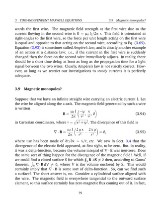
strength at the second wire due to the current flowing in the first wire is B =
µ0 I1/2π r. This field is orientated at right-angles to the second wire, so the force
per unit length exerted on the second wire is
F =
µ0 I1 I2
2π r
. (3.93)
This follows from Eq. (3.69), which is valid for continuous wires as well as short
test wires. The force acting on the second wire is directed radially inwards to-
78](https://image.slidesharecdn.com/fitzpatrick-140618223522-phpapp01/85/Fitzpatrick-r-classical-electromagnetism-78-320.jpg)
![3 TIME-INDEPENDENT MAXWELL EQUATIONS 3.10 Amp`ere’s circuital law
But, we have just demonstrated that ×B = 0. This problem is very reminiscent
of the difficulty we had earlier with · E. Recall that V · E dV = q/ 0 for a
volume V containing a discrete charge q, but that ·E = 0 at a general point. We
got around this problem by saying that ·E is a three-dimensional delta-function
whose spike is coincident with the location of the charge. Likewise, we can get
around our present difficulty by saying that × B is a two-dimensional delta-
function. A three-dimensional delta-function is a singular (but integrable) point
in space, whereas a two-dimensional delta-function is a singular line in space. It
is clear from an examination of Eqs. (3.100)–(3.102) that the only component of
×B which can be singular is the z-component, and that this can only be singular
on the z-axis (i.e., r = 0). Thus, the singularity coincides with the location of the
current, and we can write
× B = µ0 I δ(x) δ(y) ^z. (3.104)
The above equation certainly gives ( × B)x = ( × B)y = 0, and ( × B)z =
0 everywhere apart from the z-axis, in accordance with Eqs. (3.100)–(3.102).
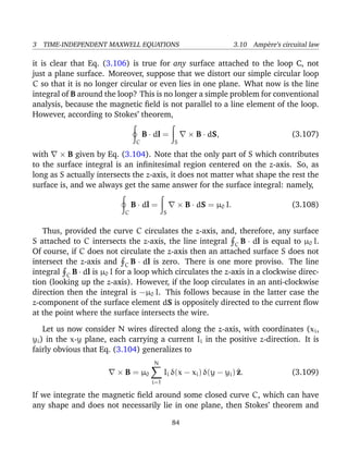
Suppose that we integrate over a plane surface S connected to the loop C. The
surface element is dS = dx dy ^z, so
S
× B · dS = µ0 I δ(x) δ(y) dx dy (3.105)
where the integration is performed over the region x2 + y2 ≤ r. However, since
the only part of S which actually contributes to the surface integral is the bit
which lies infinitesimally close to the z-axis, we can integrate over all x and y
without changing the result. Thus, we obtain
S
× B · dS = µ0 I
∞
−∞
δ(x) dx
∞
−∞
δ(y) dy = µ0 I, (3.106)
which is in agreement with Eq. (3.103).
But, why have we gone to so much trouble to prove something using vector
field theory which can be demonstrated in one line via conventional analysis
[see Eq. (3.98) ]? The answer, of course, is that the vector field result is easily
generalized, whereas the conventional result is just a special case. For instance,
83](https://image.slidesharecdn.com/fitzpatrick-140618223522-phpapp01/85/Fitzpatrick-r-classical-electromagnetism-83-320.jpg)
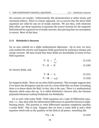
![3 TIME-INDEPENDENT MAXWELL EQUATIONS 3.11 Helmholtz’s theorem
The last three equations can be combined to form a single vector equation:
W(r) =
1
4π
C(r )
|r − r |
d3
r . (3.140)
We assumed earlier that · W = 0. Let us check to see if this is true. Note that
∂
∂x
1
|r − r |
= −
x − x
|r − r |3
=
x − x
|r − r |3
= −
∂
∂x
1
|r − r |
, (3.141)
which implies that
1
|r − r |
= −
1
|r − r |
, (3.142)
where is the operator (∂/∂x , ∂/∂y , ∂/∂z ). Taking the divergence of Eq. (3.140),
and making use of the above relation, we obtain
· W =
1
4π
C(r ) ·
1
|r − r |
d3
r = −
1
4π
C(r ) ·
1
|r − r |
d3
r . (3.143)
Now ∞
−∞
g
∂f
∂x
dx = [gf]∞
−∞ −
∞
−∞
f
∂g
∂x
dx. (3.144)
However, if g f → 0 as x → ±∞ then we can neglect the first term on the right-
hand side of the above equation and write
∞
−∞
g
∂f
∂x
dx = −
∞
−∞
f
∂g
∂x
dx. (3.145)
A simple generalization of this result yields
g · f d3
r = − f · g d3
r, (3.146)
provided that gx f → 0 as |r| → ∞, etc. Thus, we can deduce that
· W =
1
4π
·C(r )
|r − r |
d3
r (3.147)
from Eq. (3.143), provided |C(r)| is bounded as |r| → ∞. However, we have
already shown that · C = 0 from self-consistency arguments, so the above
equation implies that · W = 0, which is the desired result.
91](https://image.slidesharecdn.com/fitzpatrick-140618223522-phpapp01/85/Fitzpatrick-r-classical-electromagnetism-91-320.jpg)
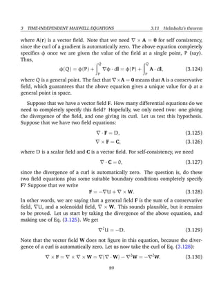
![3 TIME-INDEPENDENT MAXWELL EQUATIONS 3.11 Helmholtz’s theorem
of a conservative field and a solenoidal field. Thus, we ought to be able to write
electric and magnetic fields in this form. Second, a general vector field which is
zero at infinity is completely specified once its divergence and its curl are given.
Thus, we can guess that the laws of electromagnetism can be written as four field
equations,
· E = something, (3.151)
× E = something, (3.152)
· B = something, (3.153)
× B = something, (3.154)
without knowing the first thing about electromagnetism (other than the fact that
it deals with two vector fields). Of course, Eqs. (3.119)–(3.122) are of exactly
this form. We also know that there are only four field equations, since the above
equations are sufficient to completely reconstruct both E and B. Furthermore, we
know that we can solve the field equations without even knowing what the right-
hand sides look like. After all, we solved Eqs. (3.125)–(3.126) for completely
general right-hand sides. [Actually, the right-hand sides have to go to zero at in-
finity, otherwise integrals like Eq. (3.136) blow up.] We also know that any solu-
tions we find are unique. In other words, there is only one possible steady electric
and magnetic field which can be generated by a given set of stationary charges
and steady currents. The third thing which we proved was that if the right-hand
sides of the above field equations are all zero then the only physical solution is
E = B = 0. This implies that steady electric and magnetic fields cannot generate
themselves. Instead, they have to be generated by stationary charges and steady
currents. So, if we come across a steady electric field we know that if we trace
the field-lines back we shall eventually find a charge. Likewise, a steady mag-
netic field implies that there is a steady current flowing somewhere. All of these
results follow from vector field theory (i.e., from the general properties of fields
in three-dimensional space), prior to any investigation of electromagnetism.
93](https://image.slidesharecdn.com/fitzpatrick-140618223522-phpapp01/85/Fitzpatrick-r-classical-electromagnetism-93-320.jpg)
![3 TIME-INDEPENDENT MAXWELL EQUATIONS 3.12 The magnetic vector potential
We wish to find a vector potential A whose curl is equal to the above magnetic
field, and whose divergence is zero. It is not difficult to see that
A = −
µ0 I
4π
0, 0, ln[x2
+ y2
] (3.165)
fits the bill. Note that the vector potential is parallel to the direction of the cur-
rent. This would seem to suggest that there is a more direct relationship between
the vector potential and the current than there is between the magnetic field and
the current. The potential is not very well-behaved on the z-axis, but this is just
because we are dealing with an infinitely thin current.
Let us take the curl of Eq. (3.158). We find that
× B = × × A = ( · A) − 2
A = − 2
A, (3.166)
where use has been made of the Coulomb gauge condition (3.161). We can
combine the above relation with the field equation (3.114) to give
2
A = −µ0 j. (3.167)
Writing this in component form, we obtain
2
Ax = −µ0 jx, (3.168)
2
Ay = −µ0 jy, (3.169)
2
Az = −µ0 jz. (3.170)
But, this is just Poisson’s equation three times over. We can immediately write the
unique solutions to the above equations:
Ax(r) =
µ0
4π
jx(r )
|r − r |
d3
r , (3.171)
Ay(r) =
µ0
4π
jy(r )
|r − r |
d3
r , (3.172)
Az(r) =
µ0
4π
jz(r )
|r − r |
d3
r . (3.173)
These solutions can be recombined to form a single vector solution
A(r) =
µ0
4π
j(r )
|r − r |
d3
r . (3.174)
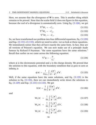
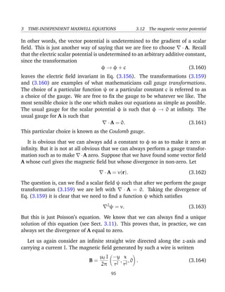
96](https://image.slidesharecdn.com/fitzpatrick-140618223522-phpapp01/85/Fitzpatrick-r-classical-electromagnetism-96-320.jpg)
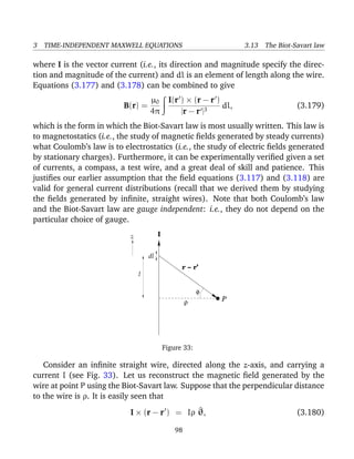
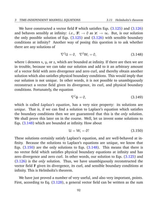
![3 TIME-INDEPENDENT MAXWELL EQUATIONS 3.14 Electrostatics and magnetostatics
l = ρ tan φ, (3.181)
dl =
ρ
cos2 φ
dφ, (3.182)
|r − r | =
ρ
cos φ
. (3.183)
Thus, according to Eq. (3.179), we have
Bθ =
µ0
4π
π/2
−π/2
I ρ
ρ3 (cos φ)−3
ρ
cos2 φ
dφ
=
µ0 I
4π ρ
π/2
−π/2
cos φ dφ =
µ0 I
4π ρ
[sin φ]
π/2
−π/2 , (3.184)
which gives the familiar result
Bθ =
µ0 I
2π ρ
. (3.185)
So, we have come full circle in our investigation of magnetic fields. Note that
the simple result (3.185) can only be obtained from the Biot-Savart law after
some non-trivial algebra. Examination of more complicated current distributions
using this law invariably leads to lengthy, involved, and extremely unpleasant
calculations.
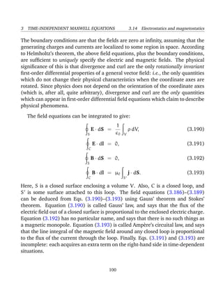
3.14 Electrostatics and magnetostatics
We have now completed our theoretical investigation of electrostatics and mag-
netostatics. Our next task is to incorporate time variation into our analysis. How-
ever, before we start this, let us briefly review our progress so far. We have found
that the electric fields generated by stationary charges, and the magnetic fields
generated by steady currents, are describable in terms of four field equations:
· E =
ρ
0
, (3.186)
× E = 0, (3.187)
· B = 0, (3.188)
× B = µ0 j. (3.189)
99](https://image.slidesharecdn.com/fitzpatrick-140618223522-phpapp01/85/Fitzpatrick-r-classical-electromagnetism-99-320.jpg)
![4 TIME-DEPENDENT MAXWELL’S EQUATIONS 4.4 Gauge transformations
be reconciled? The crucial point is that the scalar potential cannot be measured
directly, it can only be inferred from the electric field. In the time-dependent case,
there are two parts to the electric field: that part which comes from the scalar
potential, and that part which comes from the vector potential [see Eq. (4.24) ].
So, if the scalar potential responds immediately to some distance rearrangement
of charge density it does not necessarily follow that the electric field also has an
immediate response. What actually happens is that the change in the part of the
electric field which comes from the scalar potential is balanced by an equal and
opposite change in the part which comes from the vector potential, so that the
overall electric field remains unchanged. This state of affairs persists at least until
sufficient time has elapsed for a light signal to travel from the distant charges to
the region in question. Thus, relativity is not violated, since it is the electric field,
and not the scalar potential, which carries physically accessible information.
It is clear that the apparent action at a distance nature of Eq. (4.28) is highly
misleading. This suggests, very strongly, that the Coulomb gauge is not the opti-
mum gauge in the time-dependent case. A more sensible choice is the so called
Lorentz gauge:
· A = − 0µ0
∂φ
∂t
. (4.29)
It can be shown, by analogy with earlier arguments (see Sect. 3.12), that it is
always possible to make a gauge transformation, at a given instance in time, such
that the above equation is satisfied. Substituting the Lorentz gauge condition into
Eq. (4.26), we obtain
0µ0
∂2
φ
∂t2
− 2
φ =
ρ
0
. (4.30)
It turns out that this is a three-dimensional wave equation in which information
propagates at the speed of light. But, more of this later. Note that the magnet-
ically induced part of the electric field (i.e., −∂A/∂t) is not purely solenoidal in
the Lorentz gauge. This is a slight disadvantage of the Lorentz gauge with respect
to the Coulomb gauge. However, this disadvantage is more than offset by other
advantages which will become apparent presently. Incidentally, the fact that the
part of the electric field which we ascribe to magnetic induction changes when we
change the gauge suggests that the separation of the field into magnetically in-
duced and charge induced components is not unique in the general time-varying
112](https://image.slidesharecdn.com/fitzpatrick-140618223522-phpapp01/85/Fitzpatrick-r-classical-electromagnetism-112-320.jpg)
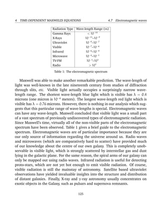
![4 TIME-DEPENDENT MAXWELL’S EQUATIONS 4.7 Electromagnetic waves
where use has been made of Eq. (4.87). A similar equation can obtained for the
electric field by taking the curl of Eq. (4.63):
2
−
1
c2
∂2
∂t2
E = 0, (4.93)
We have found that electric and magnetic fields both satisfy equations of the
form
2
−
1
c2
∂2
∂t2
A = 0 (4.94)
in free space. As is easily verified, the most general solution to this equation (with
a positive frequency) is
Ax = Fx(k · r − k c t), (4.95)
Ay = Fy(k · r − k c t), (4.96)
Az = Fz(k · r − k c t), (4.97)
where Fx(φ), Fy(φ), and Fz(φ) are one-dimensional scalar functions. Looking
along the direction of the wave-vector, so that r = (k/k) r, we find that
Ax = Fx[ k (r − c t) ], (4.98)
Ay = Fy[ k (r − c t) ], (4.99)
Az = Fz[ k (r − c t) ]. (4.100)
The x-component of this solution is shown schematically in Fig. 36. It clearly
propagates in r with velocity c. If we look along a direction which is perpendic-
ular to k then k · r = 0, and there is no propagation. Thus, the components of
A are arbitrarily shaped pulses which propagate, without changing shape, along
the direction of k with velocity c. These pulses can be related to the sinusoidal
plane-wave solutions which we found earlier by Fourier transformation. Thus,
any arbitrary shaped pulse propagating in the direction of k with velocity c can
be broken down into lots of sinusoidal oscillations propagating in the same direc-
tion with the same velocity.
The operator
2
−
1
c2
∂2
∂t2
(4.101)
127](https://image.slidesharecdn.com/fitzpatrick-140618223522-phpapp01/85/Fitzpatrick-r-classical-electromagnetism-127-320.jpg)
![4 TIME-DEPENDENT MAXWELL’S EQUATIONS 4.9 Retarded potentials
the former. According to Eqs. (4.140) and (4.141), if we want to work out the
potentials at position r and time t then we have to perform integrals of the charge
density and current density over all space (just like in the steady-state situation).
However, when we calculate the contribution of charges and currents at position
r to these integrals we do not use the values at time t, instead we use the values
at some earlier time t − |r − r |/c. What is this earlier time? It is simply the latest
time at which a light signal emitted from position r would be received at position
r before time t. This is called the retarded time. Likewise, the potentials (4.140)
and (4.141) are called retarded potentials. It is often useful to adopt the following
notation
A(r , t − |r − r |/c) ≡ [A(r , t)] . (4.142)
The square brackets denote retardation (i.e., using the retarded time instead of
the real time). Using this notation Eqs. (4.140) and (4.141), become
φ(r) =
1
4π 0
[ρ(r )]
|r − r |
d3
r , (4.143)
A(r) =
µ0
4π
[j(r )]
|r − r |
d3
r . (4.144)
The time dependence in the above equations is taken as read.
We are now in a position to understand electromagnetism at its most funda-
mental level. A charge distribution ρ(r, t) can be thought of as built up out of
a collection, or series, of charges which instantaneously come into existence, at
some point r and some time t , and then disappear again. Mathematically, this
is written
ρ(r, t) = δ(r − r )δ(t − t ) ρ(r , t ) d3
r dt . (4.145)
Likewise, we can think of a current distribution j(r, t) as built up out of a collec-
tion or series of currents which instantaneously appear and then disappear:
j(r, t) = δ(r − r )δ(t − t ) j(r , t ) d3
r dt . (4.146)
Each of these ephemeral charges and currents excites a spherical wave in the
appropriate potential. Thus, the charge density at r and t sends out a wave in
134](https://image.slidesharecdn.com/fitzpatrick-140618223522-phpapp01/85/Fitzpatrick-r-classical-electromagnetism-134-320.jpg)
![4 TIME-DEPENDENT MAXWELL’S EQUATIONS 4.9 Retarded potentials
the scalar potential:
φ(r, t) =
ρ(r , t )
4π 0
δ(t − t − |r − r |/c)
|r − r |
. (4.147)
Likewise, the current density at r and t sends out a wave in the vector potential:
A(r, t) =
µ0 j(r , t )
4π
δ(t − t − |r − r |/c)
|r − r |
. (4.148)
These waves can be thought of as messengers which inform other charges and
currents about the charges and currents present at position r and time t . How-
ever, these messengers travel at a finite speed: i.e., the speed of light. So, by the
time they reach other charges and currents their message is a little out of date. Ev-
ery charge and every current in the Universe emits these spherical waves. The re-
sultant scalar and vector potential fields are given by Eqs. (4.143) and (4.144). Of
course, we can turn these fields into electric and magnetic fields using Eqs. (4.52)
and (4.53). We can then evaluate the force exerted on charges using the Lorentz
formula. We can see that we have now escaped from the apparent action at a
distance nature of Coulomb’s law and the Biot-Savart law. Electromagnetic in-
formation is carried by spherical waves in the vector and scalar potentials, and,
therefore, travels at the velocity of light. Thus, if we change the position of a
charge then a distant charge can only respond after a time delay sufficient for a
spherical wave to propagate from the former to the latter charge.
Let us compare the steady-state law
φ(r) =
1
4π 0
ρ(r )
|r − r |
d3
r (4.149)
with the corresponding time-dependent law
φ(r) =
1
4π 0
[ρ(r )]
|r − r |
d3
r (4.150)
These two formulae look very similar indeed, but there is an important differ-
ence. We can imagine (rather pictorially) that every charge in the Universe is
continuously performing the integral (4.150), and is also performing a similar
integral to find the vector potential. After evaluating both potentials, the charge
135](https://image.slidesharecdn.com/fitzpatrick-140618223522-phpapp01/85/Fitzpatrick-r-classical-electromagnetism-135-320.jpg)
![4 TIME-DEPENDENT MAXWELL’S EQUATIONS 4.9 Retarded potentials
can calculate the fields, and, using the Lorentz force law, it can then work out
its equation of motion. The problem is that the information the charge receives
from the rest of the Universe is carried by our spherical waves, and is always
slightly out of date (because the waves travel at a finite speed). As the charge
considers more and more distant charges or currents, its information gets more
and more out of date. (Similarly, when astronomers look out to more and more
distant galaxies in the Universe, they are also looking backwards in time. In fact,
the light we receive from the most distant observable galaxies was emitted when
the Universe was only about one third of its present age.) So, what does our
electron do? It simply uses the most up to date information about distant charges
and currents which it possesses. So, instead of incorporating the charge density
ρ(r, t) in its integral, the electron uses the retarded charge density [ρ(r, t)] (i.e.,
the density evaluated at the retarded time). This is effectively what Eq. (4.150)
says.
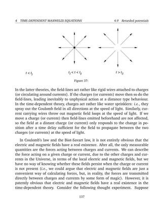
Consider a thought experiment in which a charge q appears at position r0 at
time t1, persists for a while, and then disappears at time t2. What is the electric
field generated by such a charge? Using Eq. (4.150), we find that
φ(r) =
q
4π 0
1
|r − r0|
for t1 ≤ t − |r − r0|/c ≤ t2
= 0 otherwise. (4.151)
Now, E = − φ (since there are no currents, and therefore no vector potential is
generated), so
E(r) =
q
4π 0
r − r0
|r − r0|3
for t1 ≤ t − |r − r0|/c ≤ t2
= 0 otherwise. (4.152)
This solution is shown pictorially in Fig. 37. We can see that the charge effectively
emits a Coulomb electric field which propagates radially away from the charge
at the speed of light. Likewise, it is easy to show that a current carrying wire
effectively emits an Amp`erian magnetic field at the speed of light.
We can now appreciate the essential difference between time-dependent elec-
tromagnetism and the action at a distance laws of Coulomb and Biot & Savart.
136](https://image.slidesharecdn.com/fitzpatrick-140618223522-phpapp01/85/Fitzpatrick-r-classical-electromagnetism-136-320.jpg)
![4 TIME-DEPENDENT MAXWELL’S EQUATIONS 4.11 Retarded fields
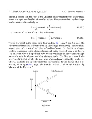
If we add the waves emitted by the charge to the response of “the rest of the
Universe” we obtain
F = F + R = (retarded). (4.163)
Thus, charges appear to emit only retarded waves, which agrees with our every-
day experience. Clearly, in this model we have side-stepped the problem of a
time asymmetric Green’s function by adopting time asymmetric boundary condi-
tions to the Universe: i.e., the distant charges in the Universe absorb retarded
waves and reflect advanced waves. This is possible because the absorption takes
place at the end of the Universe (i.e., at the “big crunch,” or whatever) and the
reflection takes place at the beginning of the Universe (i.e., at the “big bang”). It
is quite plausible that the state of the Universe (and, hence, its interaction with
electromagnetic waves) is completely different at these two times. It should be
pointed out that the Feynman-Wheeler model runs into trouble when one tries to
combine electromagnetism with quantum mechanics. These difficulties have yet
to be resolved, so at present the status of this model is that it is “an interesting
idea,” but it is still not fully accepted into the canon of physics.
4.11 Retarded fields
We know the solution to Maxwell’s equations in terms of retarded potentials. Let
us now construct the associated electric and magnetic fields using
E = − φ −
∂A
∂t
, (4.164)
B = × A. (4.165)
It is helpful to write
R = r − r , (4.166)
where R = |r−r |. The retarded time becomes tr = t−R/c, and a general retarded
quantity is written [F(r, t)] ≡ F(r, tr). Thus, we can write the retarded potential
solutions of Maxwell’s equations in the especially compact form:
φ =
1
4π 0
[ρ]
R
dV , (4.167)
143](https://image.slidesharecdn.com/fitzpatrick-140618223522-phpapp01/85/Fitzpatrick-r-classical-electromagnetism-143-320.jpg)
![4 TIME-DEPENDENT MAXWELL’S EQUATIONS 4.11 Retarded fields
A =
µ0
4π
[j]
R
dV , (4.168)
where dV ≡ d3
r .
It is easily seen that
φ =
1
4π 0
[ρ] (R−1
) +
[∂ρ/∂t]
R
tr
dV
= −
1
4π 0
[ρ]
R3
R +
[∂ρ/∂t]
cR2
R
dV , (4.169)
where use has been made of
R =
R
R
, (R−1
) = −
R
R3
, tr = −
R
cR
. (4.170)
Likewise,
× A =
µ0
4π
(R−1
) × [j] +
tr × [∂j/∂t]
R
dV
= −
µ0
4π
R × [j]
R3
+
R × [∂j/∂t]
cR2
dV . (4.171)
Equations (4.164), (4.165), (4.169), and (4.171) can be combined to give
E =
1
4π 0
[ρ]
R
R3
+
∂ρ
∂t
R
cR2
−
[∂j/∂t]
c2R
dV , (4.172)
which is the time-dependent generalization of Coulomb’s law, and
B =
µ0
4π
[j] × R
R3
+
[∂j/∂t] × R
cR2
dV , (4.173)
which is the time-dependent generalization of the Biot-Savart law.
Suppose that the typical variation time-scale of our charges and currents is t0.
Let us define R0 = c t0, which is the distance a light ray travels in time t0. We can
evaluate Eqs. (4.172) and (4.173) in two asymptotic limits: the near field region
R R0, and the far field region R R0. In the near field region
|t − tr|
t0
=
R
R0
1, (4.174)
144](https://image.slidesharecdn.com/fitzpatrick-140618223522-phpapp01/85/Fitzpatrick-r-classical-electromagnetism-144-320.jpg)
![4 TIME-DEPENDENT MAXWELL’S EQUATIONS 4.11 Retarded fields
so the difference between retarded time and standard time is relatively small.
This allows us to expand retarded quantities in a Taylor series. Thus,
[ρ] ρ +
∂ρ
∂t
(tr − t) +
1
2
∂2
ρ
∂t2
(tr − t)2
+ · · · , (4.175)
giving
[ρ] ρ −
∂ρ
∂t
R
c
+
1
2
∂2
ρ
∂t2
R2
c2
+ · · · . (4.176)
Expansion of the retarded quantities in the near field region yields
E
1
4π 0
ρ R
R3
−
1
2
∂2
ρ
∂t2
R
c2R
−
∂j/∂t
c2R
+ · · ·
dV , (4.177)
B
µ0
4π
j × R
R3
−
1
2
(∂2
j/∂t2
) × R
c2R
+ · · ·
dV . (4.178)
In Eq. (4.177), the first term on the right-hand side corresponds to Coulomb’s law,
the second term is the correction due to retardation effects, and the third term
corresponds to Faraday induction. In Eq. (4.178), the first term on the right-hand
side is the Biot-Savart law, and the second term is the correction due to retarda-
tion effects. Note that the retardation corrections are only of order (R/R0)2
. We
might suppose, from looking at Eqs. (4.172) and (4.173), that the corrections
should be of order R/R0. However, all of the order R/R0 terms canceled out in
the previous expansion. Suppose, then, that we have a d.c. circuit sitting on a
laboratory benchtop. Let the currents in the circuit change on a typical time-scale
of one tenth of a second. In this time, light can travel about 3 × 10⁷
meters, so
R0 ∼ 30, 000 kilometers. The length-scale of the experiment is about one meter,
so R = 1 meter. Thus, the retardation corrections are of order (3 × 10⁷
)−2
∼ 10−15
.
It is clear that we are fairly safe just using Coulomb’s law, Faraday’s law, and the
Biot-Savart law to analyze the fields generated by this type of circuit.
In the far field region, R R0, Eqs. (4.172) and (4.173) are dominated by the
terms which vary like R−1
, so
E −
1
4π 0
[∂j⊥/∂t]
c2 R
dV , (4.179)
B
µ0
4π
[∂j⊥/∂t] × R
c R2
dV , (4.180)
145](https://image.slidesharecdn.com/fitzpatrick-140618223522-phpapp01/85/Fitzpatrick-r-classical-electromagnetism-145-320.jpg)
![4 TIME-DEPENDENT MAXWELL’S EQUATIONS 4.11 Retarded fields
where
j⊥ = j −
(j · R)
R2
R. (4.181)
Here, use has been made of [∂ρ/∂t] = −[ · j] and [ · j] = −[∂j/∂t] · R/cR +
O(1/R2
). Suppose that our charges and currents are localized to some region in
the vicinity of r = r∗. Let R∗ = r − r∗, with R∗ = |r − r∗|. Suppose that the extent
of the current and charge containing region is much less than R∗. It follows that
retarded quantities can be written
[ρ(r, t)] ρ(r, t − R∗/c), (4.182)
etc. Thus, the electric field reduces to
E −
1
4π 0
∂j⊥/∂t dV
c2R∗
, (4.183)
whereas the magnetic field is given by
B
1
4π 0
∂j⊥/∂t dV × R∗
c3R 2
∗
. (4.184)
Note that
E
B
= c, (4.185)
and
E · B = 0. (4.186)
This configuration of electric and magnetic fields is characteristic of an electro-
magnetic wave (see Sect. 4.7). Thus, Eqs. (4.183) and (4.184) describe an elec-
tromagnetic wave propagating radially away from the charge and current con-
taining region. Note that the wave is driven by time-varying electric currents.
Now, charges moving with a constant velocity constitute a steady current, so a
non-steady current is associated with accelerating charges. We conclude that ac-
celerating electric charges emit electromagnetic waves. The wave fields, (4.183)
and (4.184), fall off like the inverse of the distance from the wave source. This
behaviour should be contrasted with that of Coulomb or Biot-Savart fields, which
fall off like the inverse square of the distance from the source. The fact that wave
fields attenuate fairly gently with increasing distance from the source is what
146](https://image.slidesharecdn.com/fitzpatrick-140618223522-phpapp01/85/Fitzpatrick-r-classical-electromagnetism-146-320.jpg)
![4 TIME-DEPENDENT MAXWELL’S EQUATIONS 4.12 Summary
B = × A. (4.196)
This prescription is not unique (there are many choices of φ and A which gen-
erate the same fields) but we can make it unique by adopting the following con-
ventions:
φ(r) → 0 as |r| → ∞, (4.197)
and
1
c2
∂φ
∂t
+ · A = 0. (4.198)
Equations (4.187) and (4.190) reduce to
22
φ = −
ρ
0
, (4.199)
22
A = −µ0 j. (4.200)
These are driven wave equations of the general form
22
u ≡
2
−
1
c2
∂2
∂t2
u = v. (4.201)
The Green’s function for this equation which satisfies the boundary conditions
and is consistent with causality is
G(r, r ; t, t ) = −
1
4π
δ(t − t − |r − r |/c)
|r − r |
. (4.202)
Thus, the solutions to Eqs. (4.199) and (4.200) are
φ(r, t) =
1
4π 0
[ρ]
R
dV , (4.203)
A(r, t) =
µ0
4π
[j]
R
dV , (4.204)
where R = |r − r |, and dV = d3
r , with [A] ≡ A(r , t − R/c). These solutions can
be combined with Eqs. (4.195) and (4.196) to give
E(r, t) =
1
4π 0
[ρ]
R
R3
+
∂ρ
∂t
R
c R2
−
[∂j/∂t]
c2 R
dV , (4.205)
B(r, t) =
µ0
4π
[j] × R
R3
+
[∂j/∂t] × R
c R2
dV . (4.206)
148](https://image.slidesharecdn.com/fitzpatrick-140618223522-phpapp01/85/Fitzpatrick-r-classical-electromagnetism-148-320.jpg)
![4 TIME-DEPENDENT MAXWELL’S EQUATIONS 4.12 Summary
Equations (4.187)–(4.206) constitute the complete theory of classical electro-
magnetism. We can express the same information in terms of field equations
[Eqs. (4.187)–(4.190)], integrated field equations [Eqs. (4.191)–(4.194)], re-
tarded electromagnetic potentials [Eqs. (4.203) and (4.204)], and retarded elec-
tromagnetic fields [Eqs. (4.205) and (4.206)]. Let us now consider the applica-
tions of this theory.
149](https://image.slidesharecdn.com/fitzpatrick-140618223522-phpapp01/85/Fitzpatrick-r-classical-electromagnetism-149-320.jpg)
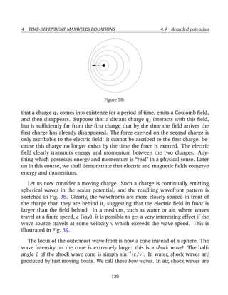
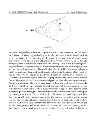
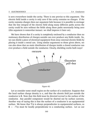
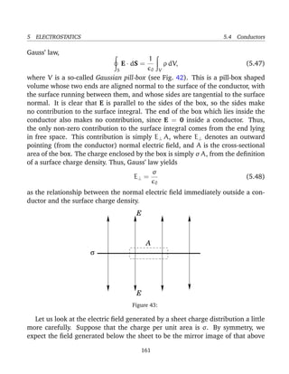
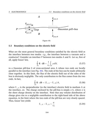
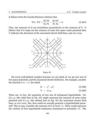
![5 ELECTROSTATICS
5 Electrostatics
5.1 Introduction
In this section, we shall use Maxwell’s equations to investigate the electric fields
generated by stationary charge distributions.
5.2 Electrostatic energy
Consider a collection of N static point charges qi located at position vectors ri
(where i runs from 1 to N). What is the electrostatic energy stored in such a
collection? Another way of asking this is, how much work would we have to do
in order to assemble the charges, starting from an initial state in which they are
all at rest and very widely separated?
We know that a static electric field is conservative, and can consequently be
written in terms of a scalar potential:
E = − φ. (5.1)
We also know that the electric force on a charge q is written
f = q E. (5.2)
The work we would have to do against electrical forces in order to move the
charge from point P to point Q is simply
W = −
Q
P
f · dl = −q
Q
P
E · dl = q
Q
P
φ · dl = q [φ(Q) − φ(P)] . (5.3)
The negative sign in the above expression comes about because we would have
to exert a force −f on the charge, in order to counteract the force exerted by the
electric field. Recall that the scalar potential generated by a point charge q at
position r is
φ(r) =
1
4π 0
q
|r − r |
. (5.4)
150](https://image.slidesharecdn.com/fitzpatrick-140618223522-phpapp01/85/Fitzpatrick-r-classical-electromagnetism-150-320.jpg)
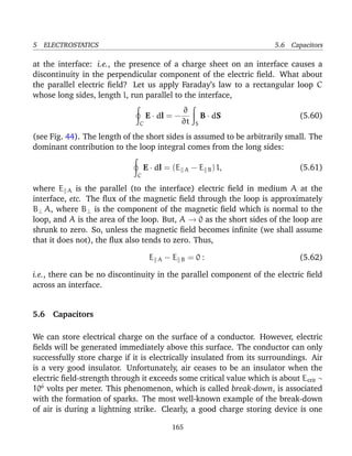
![5 ELECTROSTATICS 5.10 The method of images
Note, however, that
φanalogue(z = 0) = 0, (5.138)
and
φanalogue → 0 (5.139)
as x2
+y2
+z2
→ ∞. In addition, φanalogue satisfies Poisson’s equation for a charge
at (0, 0, d), in the region z > 0. Thus, φanalogue is a solution to the problem posed
earlier, in the region z > 0. Now, the uniqueness theorem tells us that there is
only one solution to Poisson’s equation which satisfies a given, well-posed set of
boundary conditions. So, φanalogue must be the correct potential in the region
z > 0. Of course, φanalogue is completely wrong in the region z < 0. We know
this because the grounded plate shields the region z < 0 from the point charge,
so that φ = 0 in this region. Note that we are leaning pretty heavily on the
uniqueness theorem here! Without this theorem, it would be hard to convince a
skeptical person that φ = φanalogue is the correct solution in the region z > 0.
Now that we know the potential in the region z > 0, we can easily work out the
distribution of charges induced on the conducting plate. We already know that
the relation between the electric field immediately above a conducting surface
and the density of charge on the surface is
E⊥ =
σ
0
. (5.140)
In this case,
E⊥ = Ez(z = 0+) = −
∂φ(z = 0+)
∂z
= −
∂φanalogue(z = 0+)
∂z
, (5.141)
so
σ = − 0
∂φanalogue(z = 0+)
∂z
. (5.142)
It follows from Eq. (5.137) that
∂φ
∂z
=
q
4π 0
−(z − d)
[x2 + y2 + (z − d)2]3/2
+
(z + d)
[x2 + y2 + (z + d)2]3/2
, (5.143)
so
σ(x, y) = −
q d
2π (x2 + y2 + d2)3/2
. (5.144)
179](https://image.slidesharecdn.com/fitzpatrick-140618223522-phpapp01/85/Fitzpatrick-r-classical-electromagnetism-179-320.jpg)
![5 ELECTROSTATICS 5.10 The method of images
Of course, this work is equivalent to the potential energy we evaluated earlier,
and is, in turn, the same as the energy contained in the electric field.
As a second example of the method of images, consider a grounded spherical
conductor of radius a placed at the origin. Suppose that a charge q is placed
outside the sphere at (b, 0, 0), where b > a. What is the force of attraction
between the sphere and the charge? In this case, we proceed by considering an
analogue problem in which the sphere is replaced by an image charge −q placed
somewhere on the x-axis at (c, 0, 0). The electric potential throughout space in
the analogue problem is simply
φ =
q
4π 0
1
[(x − b)2 + y2 + z2]1/2
−
q
4π 0
1
[(x − c)2 + y2 + z2]1/2
. (5.159)
The image charge is chosen so as to make the surface φ = 0 correspond to the
surface of the sphere. Setting the above expresion to zero, and performing a little
algebra, we find that the φ = 0 surface satisfies
x2
+
2 (c − λ b)
λ − 1
x + y2
+ z2
=
c2
− λ b2
λ − 1
, (5.160)
where λ = q 2
/q2
. Of course, the surface of the sphere satisfies
x2
+ y2
+ z2
= a2
. (5.161)
The above two equations can be made identical by setting λ = c/b and a2
= λ b2
,
or
q =
a
b
q, (5.162)
and
c =
a2
b
. (5.163)
According to the uniqueness theorem, the potential in the analogue problem is
now identical with that in the real problem, outside the sphere. (Of course, in
the real problem, the potential inside the sphere is zero.) Hence, the force of
attraction between the sphere and the original charge in the real problem is the
same as the force of attraction between the two charges in the analogue problem.
It follows that
f =
q q
4π 0 (b − c)2
=
q2
4π 0
a b
(b2 − a2)2
. (5.164)
182](https://image.slidesharecdn.com/fitzpatrick-140618223522-phpapp01/85/Fitzpatrick-r-classical-electromagnetism-182-320.jpg)
![5 ELECTROSTATICS 5.12 Separation of variables
This equation has the form
f(x) = g(y), (5.204)
where f and g are general functions. The only way in which the above equa-
tion can be satisfied, for general x and y, is if both sides are equal to the same
constant. Thus,
1
X
d2
X
dx2
= k2
= −
1
Y
d2
Y
dy2
. (5.205)
The reason why we write k2
, rather than −k2
, will become apparent later on.
Equation (5.205) separates into two ordinary differential equations:
d2
X
dx2
= k2
X, (5.206)
d2
Y
dy2
= −k2
Y. (5.207)
We know the general solution to these equations:
X = A exp(k x) + B exp(−k x), (5.208)
Y = C sin(k y) + D cos(k y), (5.209)
giving
φ = [ A exp(k x) + B exp(−k x) ] [C sin(k y) + D cos(k y)]. (5.210)
Here, A, B, C, and D are arbitrary constants. The boundary condition (5.200)
is automatically satisfied if A = 0 and k > 0. Note that the choice k2
, instead of
−k2
, in Eq. (5.205) facilitates this by making φ either grow or decay monoton-
ically in the x-direction instead of oscillating. The boundary condition (5.197)
is automatically satisfied if D = 0. The boundary condition (5.198) is satisfied
provided that
sin(k π) = 0, (5.211)
which implies that k is a positive integer, n (say). So, our solution reduces to
φ(x, y) = C exp(−n x) sin(n y), (5.212)
where B has been absorbed into C. Note that this solution is only able to satisfy
the final boundary condition (5.199) provided φ0(y) is proportional to sin(n y).
190](https://image.slidesharecdn.com/fitzpatrick-140618223522-phpapp01/85/Fitzpatrick-r-classical-electromagnetism-190-320.jpg)
![5 ELECTROSTATICS 5.12 Separation of variables
so
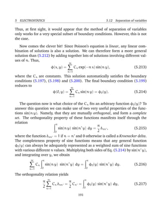
Cn =
2
π
π
0
φ0(y) sin(n y) dy. (5.218)
Thus, we now have a general solution to the problem for any driving potential
φ0(y).
If the potential φ0(y) is constant then
Cn =
2 φ0
π
π
0
sin(n y) dy =
2 φ0
n π
[1 − cos(n π)], (5.219)
giving
Cn = 0 (5.220)
for even n, and
Cn =
4 φ0
n π
(5.221)
for odd n. Thus,
φ(x, y) =
4 φ0
π n=1,3,5
exp(−n x) sin(n y)
n
. (5.222)
In the above problem, we write the potential as the product of one-dimensional
functions. Some of these functions grow and decay monotonically (i.e., the ex-
ponential functions), and the others oscillate (i.e., the sinusoidal functions). The
success of the method depends crucially on the orthogonality and completeness
of the oscillatory functions. A set of functions fn(x) is orthogonal if the integral of
the product of two different members of the set over some range is always zero:
i.e.,
b
a
fn(x) fm(x) dx = 0, (5.223)
for n = m. A set of functions is complete if any other function can be expanded
as a weighted sum of them. It turns out that the scheme set out above can be
generalized to more complicated geometries. For instance, in spherical geome-
try, the monotonic functions are power law functions of the radial variable, and
the oscillatory functions are Legendre polynomials. The latter are both mutually
192](https://image.slidesharecdn.com/fitzpatrick-140618223522-phpapp01/85/Fitzpatrick-r-classical-electromagnetism-192-320.jpg)
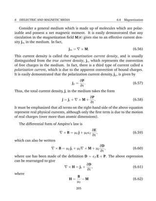
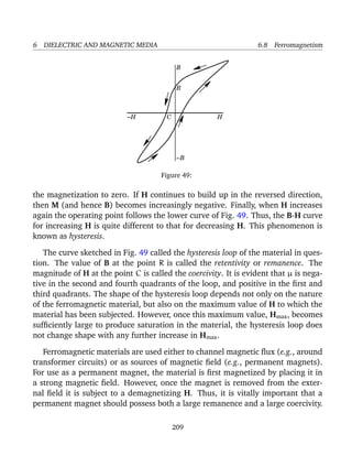
![6 DIELECTRIC AND MAGNETIC MEDIA 6.2 Polarization
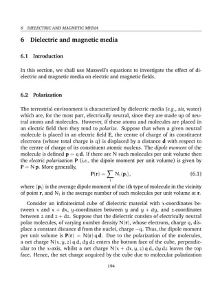
in the x-direction is dq = −N(x + dx, y, z) q dx dy dz + N(x, y, z) q dx dy dz =
−[∂N(x, y, z)/∂x] q dx dx dy dz = −[∂Px(x, y, z)/∂x] dx dy dz. There are analo-
gous contributions due to polarization in the y- and z-directions. Hence, the net
charge acquired by the cube due to molecular polarization is dq = −[∂Px(x, y, z)/∂x+
∂Py(x, y, z)/∂y+∂Pz(x, y, z)/∂z] dx dy dz = −( ·P) dx dy dz. Thus, it follows that
the charge density acquired by the cube due to molecular polarization is simply
− ·P.
As explained above, it is easily demonstrated that any divergence of the polar-
ization field P(r) of a dielectric medium gives rise to an effective charge density
ρb in the medium, where
ρb = − ·P. (6.2)
This charge density is attributable to bound charges (i.e., charges which arise from
the polarization of neutral atoms), and is usually distinguished from the charge
density ρf due to free charges, which represents a net surplus or deficit of electrons
in the medium. Thus, the total charge density ρ in the medium is
ρ = ρf + ρb. (6.3)
It must be emphasized that both terms in this equation represent real physical
charge. Nevertheless, it is useful to make the distinction between bound and
free charges, especially when it comes to working out the energy associated with
electric fields in dielectric media.
Gauss’ law takes the differential form
·E =
ρ
0
=
ρf + ρb
0
. (6.4)
This expression can be rearranged to give
·D = ρf, (6.5)
where
D = 0 E + P (6.6)
is termed the electric displacement, and has the same dimensions as P (dipole
moment per unit volume). Gauss’ theorem tells us that
S
D·dS =
V
ρf dV. (6.7)
195](https://image.slidesharecdn.com/fitzpatrick-140618223522-phpapp01/85/Fitzpatrick-r-classical-electromagnetism-195-320.jpg)
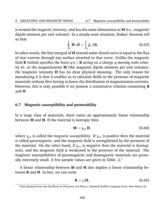
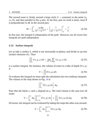
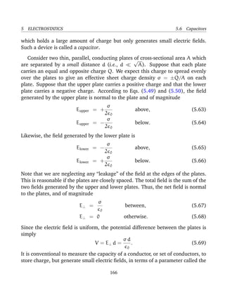
![7 MAGNETIC INDUCTION 7.3 Self-inductance
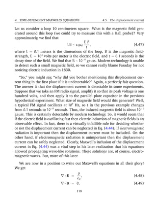
V
I
L
R
Figure 51:
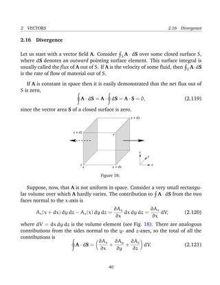
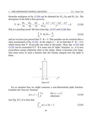
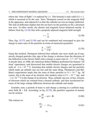
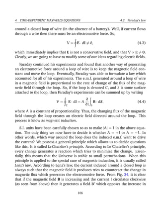
The general solution is
I(t) =
V
R
+ k exp(−R t/L). (7.18)
The constant k is fixed by the boundary conditions. Suppose that the battery is
connected at time t = 0, when I = 0. It follows that k = −V/R, so that
I(t) =
V
R
[1 − exp(−R t/L) ] . (7.19)
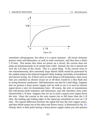
This curve is sketched in Fig. 52. It can be seen that, after the battery is con-
nected, the current ramps up, and attains its steady-state value V/R (which comes
from Ohm’s law), on the characteristic time-scale
τ =
L
R
. (7.20)
This time-scale is sometimes called the time constant of the circuit, or, somewhat
unimaginatively, the L over R time of the circuit.
We can now appreciate the significance of self-inductance. The back e.m.f.
generated in an inductor, as the current tries to change, effectively prevents the
current from rising (or falling) much faster than the L/R time. This effect is
220](https://image.slidesharecdn.com/fitzpatrick-140618223522-phpapp01/85/Fitzpatrick-r-classical-electromagnetism-220-320.jpg)
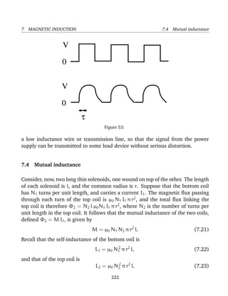
![7 MAGNETIC INDUCTION 7.4 Mutual inductance
a voltmeter of very high internal resistance, so that I2 = 0. What is the e.m.f.
generated in the top coil? Since I2 = 0, the circuit equation for the bottom coil is
V1 = R1 I1 + L1
dI1
dt
, (7.30)
where V1 is constant, and I1(t = 0) = 0. We have already seen the solution to
this equation:
I1 =
V1
R1
[1 − exp(−R1 t/L1) ] . (7.31)
The circuit equation for the top coil is
V2 = M
dI1
dt
, (7.32)
giving
V2 = V1
M
L1
exp(−R1 t/L1). (7.33)
It follows from Eq. (7.25) that
V2 = V1 k
L2
L1
exp(−R1 t/L1). (7.34)
Since L1/L2 = N2
1 /N2
2 , we obtain
V2 = V1 k
N2
N1
exp(−R1 t/L1). (7.35)
Note that V2(t) is discontinuous at t = 0. This is not a problem, since the resis-
tance of the top circuit is infinite, so there is no discontinuity in the current (and,
hence, in the magnetic field). But, what about the displacement current, which
is proportional to ∂E/∂t? Surely, this is discontinuous at t = 0 (which is clearly
unphysical)? The crucial point, here, is that we have specifically neglected the
displacement current in all of our previous analysis, so it does not make much
sense to start worrying about it now. If we had retained the displacement cur-
rent in our calculations, then we would have found that the voltage in the top
circuit jumps up, at t = 0, on a time-scale similar to the light traverse time across
the circuit (i.e., the jump is instantaneous to all intents and purposes, but the
displacement current remains finite).
224](https://image.slidesharecdn.com/fitzpatrick-140618223522-phpapp01/85/Fitzpatrick-r-classical-electromagnetism-224-320.jpg)
![7 MAGNETIC INDUCTION 7.5 Magnetic energy
I = n q, so the power output is V I.] The total work done by the battery in raising
the current in the circuit from zero at time t = 0 to IT at time t = T is
W =
T
0
VI dt. (7.38)
Using the circuit equation (7.37), we obtain
W = L
T
0
I
dI
dt
dt + R
T
0
I2
dt, (7.39)
giving
W =
1
2
L I2
T + R
T
0
I2
dt. (7.40)
The second term on the right-hand side represents the irreversible conversion of
electrical energy into heat energy in the resistor. The first term is the amount of
energy stored in the inductor at time T. This energy can be recovered after the in-
ductor is disconnected from the battery. Suppose that the battery is disconnected
at time T. The circuit equation is now
0 = L
dI
dt
+ RI, (7.41)
giving
I = IT exp −
R
L
(t − T) , (7.42)
where we have made use of the boundary condition I(T) = IT . Thus, the current
decays away exponentially. The energy stored in the inductor is dissipated as heat
in the resistor. The total heat energy appearing in the resistor after the battery is
disconnected is ∞
T
I2
R dt =
1
2
L I2
T , (7.43)
where use has been made of Eq. (7.42). Thus, the heat energy appearing in the
resistor is equal to the energy stored in the inductor. This energy is actually stored
in the magnetic field generated around the inductor.
Consider, again, our circuit with two coils wound on top of one another. Sup-
pose that each coil is connected to its own battery. The circuit equations are
226](https://image.slidesharecdn.com/fitzpatrick-140618223522-phpapp01/85/Fitzpatrick-r-classical-electromagnetism-226-320.jpg)
![7 MAGNETIC INDUCTION 7.5 Magnetic energy
Let us now examine a more general proof of the above formula. Consider a
system of N circuits (labeled i = 1 to N), each carrying a current Ii. The magnetic
flux through the ith circuit is written [cf., Eq. (7.5) ]
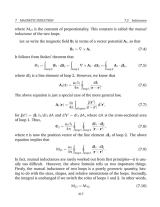
Φi = B · dSi = A · dli, (7.56)
where B = × A, and dSi and dli denote a surface element and a line element
of this circuit, respectively. The back e.m.f. induced in the ith circuit follows from
Faraday’s law:
Vi = −
dΦi
dt
. (7.57)
The rate of work of the battery which maintains the current Ii in the ith circuit
against this back e.m.f. is
Pi = Ii
dΦi
dt
. (7.58)
Thus, the total work required to raise the currents in the N circuits from zero at
time 0, to I0 i at time T, is
W =
N
i=1
T
0
Ii
dΦi
dt
dt. (7.59)
The above expression for the work done is, of course, equivalent to the total
energy stored in the magnetic field surrounding the various circuits. This energy
is independent of the manner in which the currents are set up. Suppose, for the
sake of simplicity, that the currents are ramped up linearly, so that
Ii = I0 i
t
T
. (7.60)
The fluxes are proportional to the currents, so they must also ramp up linearly:
Φi = Φ0 i
t
T
. (7.61)
It follows that
W =
N
i=1
T
0
I0 i Φ0 i
t
T2
dt, (7.62)
229](https://image.slidesharecdn.com/fitzpatrick-140618223522-phpapp01/85/Fitzpatrick-r-classical-electromagnetism-229-320.jpg)
![7 MAGNETIC INDUCTION 7.5 Magnetic energy
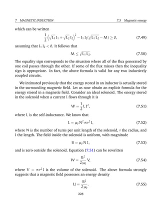
giving
W =
1
2
N
i=1
I0 i Φ0 i. (7.63)
So, if instantaneous currents Ii flow in the the N circuits, which link instanta-
neous fluxes Φi, then the instantaneous stored energy is
W =
1
2
N
i=1
Ii Φi. (7.64)
Equations (7.56) and (7.64) imply that
W =
1
2
N
i=1
Ii A · dli. (7.65)
It is convenient, at this stage, to replace our N line currents by N current dis-
tributions of small, but finite, cross-sectional area. Equation (7.65) transforms
to
W =
1
2 V
A · j dV, (7.66)
where V is a volume which contains all of the circuits. Note that for an element
of the ith circuit j = Ii dli/dli Ai and dV = dli Ai, where Ai is the cross-sectional
area of the circuit. Now, µ0 j = ×B (we are neglecting the displacement current
in this calculation), so
W =
1
2 µ0 V
A · × B dV. (7.67)
According to vector field theory,
· (A × B) ≡ B · × A − A · × B, (7.68)
which implies that
W =
1
2 µ0 V
[− · (A × B) + B · × A] dV. (7.69)
Using Gauss’ theorem, and B = × A, we obtain
W = −
1
2 µ0 S
A × B · dS +
1
2 µ0 V
B2
dV, (7.70)
230](https://image.slidesharecdn.com/fitzpatrick-140618223522-phpapp01/85/Fitzpatrick-r-classical-electromagnetism-230-320.jpg)
![7 MAGNETIC INDUCTION 7.6 Alternating current circuits
where the average is taken over one period of the oscillation. Let us, first of all,
calculate the power using real (rather than complex) voltages and currents. We
can write
V(t) = |V0| cos(ω t), (7.83)
I(t) = |I0| cos(ω t − θ), (7.84)
where θ is the phase-lag of the current with respect to the voltage. It follows that
P = |V0| |I0|
ωt=2π
ωt=0
cos(ω t) cos(ω t − θ)
d(ω t)
2π
= |V0| |I0|
ωt=2π
ωt=0
cos(ω t) [cos(ω t) cos θ + sin(ω t) sin θ]
d(ω t)
2π
,(7.85)
giving
P =
1
2
|V0| |I0| cos θ, (7.86)
since cos(ω t) sin(ω t) = 0 and cos(ω t) cos(ω t) = 1/2. In complex repre-
sentation, the voltage and the current are written
V(t) = |V0| exp(i ω t), (7.87)
I(t) = |I0| exp[i (ω t − θ)]. (7.88)
Note that
1
2
(V I∗
+ V∗
I) = |V0| |I0| cos θ. (7.89)
It follows that
P =
1
4
(V I∗
+ V∗
I) =
1
2
Re(V I∗
). (7.90)
Making use of Eq. (7.81), we find that
P =
1
2
Re(Z) |I|2
=
1
2
Re(Z) |V|2
|Z|2
. (7.91)
Note that power dissipation is associated with the real part of the impedance. For
the special case of an LCR circuit,
P =
1
2
R |I0|2
. (7.92)
233](https://image.slidesharecdn.com/fitzpatrick-140618223522-phpapp01/85/Fitzpatrick-r-classical-electromagnetism-233-320.jpg)
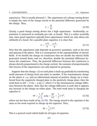
![7 MAGNETIC INDUCTION 7.7 Transmission lines
ω, is sufficiently high, then this assumption becomes invalid. The assumption of
a constant phase throughout the circuit is reasonable if the wave-length of the
oscillation, λ = 2π c/ω, is much larger than the dimensions of the circuit. (Here,
we assume that signals propagate around electrical circuits at about the velocity
of light. This assumption will be justified later on.) This is generally not the case
in electrical circuits which are associated with communication. The frequencies in
such circuits tend to be very high, and the dimensions are, almost by definition,
large. For instance, leased telephone lines (the type you attach computers to) run
at 56 kHz. The corresponding wave-length is about 5 km, so the constant-phase
approximation clearly breaks down for long-distance calls. Computer networks
generally run at about 100 MHz, corresponding to λ ∼ 3 m. Thus, the constant-
phase approximation also breaks down for most computer networks, since such
networks are generally significantly larger than 3 m. It turns out that you need
a special sort of wire, called a transmission line, to propagate signals around
circuits whose dimensions greatly exceed the wave-length, λ. Let us investigate
transmission lines.
An idealized transmission line consists of two parallel conductors of uniform
cross-sectional area. The conductors possess a capacitance per unit length, C,
and an inductance per unit length, L. Suppose that x measures the position along
the line.
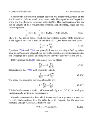
Consider the voltage difference between two neighbouring points on the line,
located at positions x and x + δx, respectively. The self-inductance of the portion
of the line lying between these two points is L δx. This small section of the line can
be thought of as a conventional inductor, and, therefore, obeys the well-known
equation
V(x, t) − V(x + δx, t) = L δx
∂I(x, t)
∂t
, (7.95)
where V(x, t) is the voltage difference between the two conductors at position x
and time t, and I(x, t) is the current flowing in one of the conductors at position
x and time t [the current flowing in the other conductor is −I(x, t) ]. In the limit
δx → 0, the above equation reduces to
∂V
∂x
= −L
∂I
∂t
. (7.96)
235](https://image.slidesharecdn.com/fitzpatrick-140618223522-phpapp01/85/Fitzpatrick-r-classical-electromagnetism-235-320.jpg)
![7 MAGNETIC INDUCTION 7.7 Transmission lines
down the line is absorbed by the resistor. What happens if R = Z0? The answer
is that some of the power is reflected back down the line. Suppose that the
beginning of the line lies at x = −l, and the end of the line is at x = 0. Let us
consider a solution
V(x, t) = V0 exp[i (ω t − k x)] + K V0 exp[i (ω t + k x)]. (7.115)
This corresponds to a voltage wave of amplitude V0 which travels down the line,
and is reflected at the end of the line, with reflection coefficient K. It is easily
demonstrated from the telegrapher’s equations that the corresponding current
waveform is
I(x, t) =
V0
Z0
exp[i (ω t − k x)] −
K V0
Z0
exp[i (ω t + k x)]. (7.116)
Since the line is terminated by a resistance R at x = 0, we have, from Ohm’s law,
V(0, t)
I(0, t)
= R. (7.117)
This yields an expression for the coefficient of reflection,
K =
R − Z0
R + Z0
. (7.118)
The input impedance of the line is given by
Zin =
V(−l, t)
I(−l, t)
= Z0
R cos(k l) + i Z0 sin(k l)
Z0 cos(k l) + i R sin(k l)
. (7.119)
Clearly, if the resistor at the end of the line is properly matched, so that R = Z0,
then there is no reflection (i.e., K = 0), and the input impedance of the line is Z0.
If the line is short-circuited, so that R = 0, then there is total reflection at the end
of the line (i.e., K = −1), and the input impedance becomes
Zin = i Z0 tan(k l). (7.120)
This impedance is purely imaginary, implying that the transmission line absorbs
no net power from the generator circuit. In fact, the line acts rather like a pure
inductor or capacitor in the generator circuit (i.e., it can store, but cannot absorb,
239](https://image.slidesharecdn.com/fitzpatrick-140618223522-phpapp01/85/Fitzpatrick-r-classical-electromagnetism-239-320.jpg)
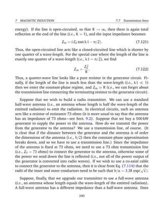
![8 ELECTROMAGNETIC ENERGY AND MOMENTUM
8 Electromagnetic energy and momentum
8.1 Introduction
In this section, we shall demonstrate that Maxwell’s equations conserve both en-
ergy and momentum.
8.2 Energy conservation
We have seen that the energy density of an electric field is given by [see Eq. (5.20)]
UE =
0 E2
2
, (8.1)
whereas the energy density of a magnetic field satisfies [see Eq. (7.55)]
UB =
B2
2 µ0
. (8.2)
This suggests that the energy density of a general electromagnetic field is
U =
0 E2
2
+
B2
2 µ0
. (8.3)
We are now in a position to demonstrate that the classical theory of electromag-
netism conserves energy. We have already come across one conservation law in
electromagnetism:
∂ρ
∂t
+ · j = 0. (8.4)
This is the equation of charge conservation. Integrating over some volume V,
bounded by a surface S, and making use of Gauss’ theorem, we obtain
−
∂
∂t V
ρ dV =
S
j · dS. (8.5)
In other words, the rate of decrease of the charge contained in volume V equals
the net flux of charge across surface S. This suggests that an energy conservation
242](https://image.slidesharecdn.com/fitzpatrick-140618223522-phpapp01/85/Fitzpatrick-r-classical-electromagnetism-242-320.jpg)
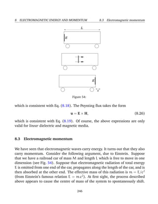
![8 ELECTROMAGNETIC ENERGY AND MOMENTUM 8.4 Momentum conservation
if the local direction of the solar wind is not radially outward from the Sun (which
is quite often the case).
The radiation pressure from sunlight is very weak. However, that produced by
laser beams can be enormous (far higher than any conventional pressure which
has ever been produced in a laboratory). For instance, the lasers used in Inertial
Confinement Fusion (e.g., the NOVA experiment in Lawrence Livermore National
Laboratory) typically have energy fluxes of 1018
W m−2
. This translates to a radi-
ation pressure of about 104
atmospheres!
8.4 Momentum conservation
It follows from Eqs. (8.19) and (8.33) that the momentum density of electromag-
netic fields can be written
g = 0 E × B. (8.41)
Now, a momentum conservation equation for electromagnetic fields should take
the integral form
−
∂
∂t V
gi dV =
S
Gij dSj +
V
[ρ E + j × B]i dV. (8.42)
Here, i and j run from 1 to 3 (1 corresponds to the x-direction, 2 to the y-
direction, and 3 to the z-direction). Moreover, the Einstein summation conven-
tion is employed for repeated indices (e.g., aj aj ≡ a · a). Furthermore, the tensor
Gij represents the flux of the ith component of electromagnetic momentum in the
j-direction. This tensor (a tensor is a direct generalization of a vector with two
indices instead of one) is called the momentum flux density. Hence, the above
equation states that the rate of loss of electromagnetic momentum in some vol-
ume V is equal to the flux of electromagnetic momentum across the bounding
surface S plus the rate at which momentum is transferred to matter inside V. The
latter rate is, of course, just the net electromagnetic force acting on matter inside
V: i.e., the volume integral of the electromagnetic force density, ρ E + j × B. Now,
a direct generalization of the divergence theorem states that
S
Gij dSj ≡
V
∂Gij
∂xj
dV, (8.43)
250](https://image.slidesharecdn.com/fitzpatrick-140618223522-phpapp01/85/Fitzpatrick-r-classical-electromagnetism-250-320.jpg)
![8 ELECTROMAGNETIC ENERGY AND MOMENTUM 8.4 Momentum conservation
where x1 ≡ x, x2 ≡ y, etc. Hence, in differential form, our momentum conserva-
tion equation for electromagnetic fields is written
−
∂
∂t
[ 0 E × B]i =
∂Gij
∂xj
+ [ρ E + j × B]i. (8.44)
Let us now attempt to derive an equation of this form from Maxwell’s equations.
Maxwell’s equations are written:
· E =
ρ
0
, (8.45)
· B = 0, (8.46)
× E = −
∂B
∂t
, (8.47)
× B = µ0 j + 0µ0
∂E
∂t
. (8.48)
We can cross Eq. (8.48) divided by µ0 with B, and rearrange, to give
− 0
∂E
∂t
× B =
B × ( × B)
µ0
+ j × B. (8.49)
Next, let us cross E with Eq. (8.47) times 0, rearrange, and add the result to the
above equation. We obtain
− 0
∂E
∂t
× B − 0 E ×
∂B
∂t
= 0 E × ( × E) +
B × ( × B)
µ0
+ j × B. (8.50)
Next, making use of Eqs. (8.45) and (8.46), we get
−
∂
∂t
[ 0 E × B] = 0 E × ( × E) +
B × ( × B)
µ0
− 0 ( · E) E −
1
µ0
( · B) B + ρ E + j × B. (8.51)
Now, from vector field theory,
(E2
/2) ≡ E × ( × E) + (E · )E, (8.52)
251](https://image.slidesharecdn.com/fitzpatrick-140618223522-phpapp01/85/Fitzpatrick-r-classical-electromagnetism-251-320.jpg)
![8 ELECTROMAGNETIC ENERGY AND MOMENTUM 8.4 Momentum conservation
with a similar equation for B. Hence, Eq. (8.51) takes the form
−
∂
∂t
[ 0 E × B] = 0 (E2
/2) − ( · E) E − (E · )E
+
1
µ0
(B2
/2) − ( · B) B − (B · )B
+ρ E + j × B. (8.53)
Finally, when written in terms of components, the above equation becomes
−
∂
∂t
[ 0 E × B]i =
∂
∂xj
0 E2
δij/2 − 0 Ei Ej + B2
δij/2 µ0 − Bi Bj/µ0
+ [ρ E + j × B]i , (8.54)
since [( · E) E]i = (∂Ej/∂xj) Ei, and [(E · )E]i = Ej (∂Ei/∂xj). Here, δij is a
Kronecker delta symbol (i.e., δij = 1 if i = j, and δij = 0 otherwise). Comparing
the above equation with Eq. (8.44), we conclude that the momentum flux density
tensor of electromagnetic fields takes the form
Gij = 0 (E2
δij/2 − Ei Ej) + (B2
δij/2 − Bi Bj)/µ0. (8.55)
The momentum conservation equation (8.44) is sometimes written
[ρ E + j × B]i =
∂Tij
∂xj
−
∂
∂t
[ 0 E × B]i , (8.56)
where
Tij = −Gij = 0 (Ei Ej − E2
δij/2) + (Bi Bj − B2
δij/2)/µ0 (8.57)
is called the Maxwell stress tensor.
252](https://image.slidesharecdn.com/fitzpatrick-140618223522-phpapp01/85/Fitzpatrick-r-classical-electromagnetism-252-320.jpg)
![9 ELECTROMAGNETIC RADIATION
9 Electromagnetic radiation
9.1 Introduction
In this section, we shall use Maxwell’s equations to investigate electromagnetic
waves.
9.2 The Hertzian dipole
Consider two small spherical conductors connected by a wire. Suppose that elec-
tric charge flows periodically back and forth between the spheres. Let q(t) be the
instantaneous charge on one of the conductors. The system has zero net charge,
so the charge on the other conductor is −q(t). Let
q(t) = q0 sin (ω t). (9.1)
We expect the oscillating current flowing in the wire connecting the two spheres
to generate electromagnetic radiation (see Sect. 4.11). Let us consider the simple
case in which the length of the wire is small compared to the wave-length of
the emitted radiation. If this is the case, then the current I flowing between the
conductors has the same phase along the whole length of the wire. It follows that
I(t) =
dq
dt
= I0 cos(ω t), (9.2)
where I0 = ω q0. This type of antenna is called a Hertzian dipole, after the
German physicist Heinrich Hertz.
The magnetic vector potential generated by a current distribution j(r) is given
by the well-known formula (see Sect. 4.12)
A(r, t) =
µ0
4π
[j]
|r − r |
d3
r , (9.3)
where
[f] = f(r , t − |r − r |/c). (9.4)
253](https://image.slidesharecdn.com/fitzpatrick-140618223522-phpapp01/85/Fitzpatrick-r-classical-electromagnetism-253-320.jpg)
![9 ELECTROMAGNETIC RADIATION 9.2 The Hertzian dipole
to leading order in r−1
. Thus,
φ(r, t)
l
4π 0 c
z
r
I(t − r/c)
r
. (9.13)
Given the vector and scalar potentials, Eqs. (9.10) and (9.13), respectively, we
can evaluate the associated electric and magnetic fields using (see Sect. 4.12)
E = −
∂A
∂t
− φ, (9.14)
B = × A. (9.15)
Note that we are only interested in radiation fields, which fall off like r−1
with
increasing distance from the source. It is easily demonstrated that
E −
ω l I0
4π 0 c2
sin θ
sin[ω(t − r/c)]
r
^θ, (9.16)
and
B −
ω l I0
4π 0 c3
sin θ
sin[ω(t − r/c)]
r
^ϕ. (9.17)
Here, (r, θ, ϕ) are standard spherical polar coordinates aligned along the z-axis.
The above expressions for the far field (i.e., r λ) electromagnetic fields gen-
erated by a localized oscillating current are also easily derived from Eqs. (4.183)
and (4.184). Note that the fields are symmetric in the azimuthal angle ϕ. There
is no radiation along the axis of the oscillating dipole (i.e., θ = 0), and the maxi-
mum emission is in the plane perpendicular to this axis (i.e., θ = π/2).
The average power crossing a spherical surface S (whose radius is much greater
than λ) is
Prad =
S
u · dS, (9.18)
where the average is over a single period of oscillation of the wave, and the
Poynting flux is given by (see Sect. 8.2)
u =
E × B
µ0
=
ω2
l2
I2
0
16π2
0 c3
sin2
[ω(t − r/c)]
sin2
θ
r2
^r. (9.19)
255](https://image.slidesharecdn.com/fitzpatrick-140618223522-phpapp01/85/Fitzpatrick-r-classical-electromagnetism-255-320.jpg)
![9 ELECTROMAGNETIC RADIATION 9.2 The Hertzian dipole
The power transferred to the load is
Pload = I2
Rload =
Rload V 2
0
2 (Rrad + Rload)2
. (9.30)
The power re-radiated by the antenna is
Prad = I2
Rrad =
Rrad V 2
0
2 (Rrad + Rload)2
. (9.31)
Note that Pin = Pload + Prad. The maximum power transfer to the load occurs
when
∂Pload
∂Rload
=
V 2
0
2
Rrad − Rload
(Rrad + Rload)3
= 0. (9.32)
Thus, the maximum transfer rate corresponds to
Rload = Rrad. (9.33)
In other words, the resistance of the load circuit must match the radiation resis-
tance of the antenna. For this optimum case,
Pload = Prad =
V 2
0
8 Rrad
=
Pin
2
. (9.34)
So, in the optimum case half of the power absorbed by the antenna is immediately
re-radiated. Clearly, an antenna which is receiving electromagnetic radiation is
also emitting it. This is how the BBC catch people who do not pay their television
license fee in England. They have vans which can detect the radiation emitted by
a TV aerial whilst it is in use (they can even tell which channel you are watching!).
For a Hertzian dipole antenna interacting with an incoming wave whose elec-
tric field has an amplitude E0, we expect
V0 = E0 l. (9.35)
Here, we have used the fact that the wave-length of the radiation is much longer
than the length of the antenna. We have also assumed that the antenna is prop-
erly aligned (i.e., the radiation is incident perpendicular to the axis of the an-
tenna). The Poynting flux of the incoming wave is [see Eq. (8.35)]
uin =
0 c E2
0
2
, (9.36)
258](https://image.slidesharecdn.com/fitzpatrick-140618223522-phpapp01/85/Fitzpatrick-r-classical-electromagnetism-258-320.jpg)
![9 ELECTROMAGNETIC RADIATION 9.4 Thompson scattering
where p0 = q0 l = I0 l/ω. We found that, in the far field, the mean electromag-
netic energy flux takes the form [see Eq. (9.20)]
u =
ω4
p2
0
32π2
0 c3
sin2
θ
r2
^r, (9.43)
assuming that the dipole is centered on the origin of our spherical polar coor-
dinate system. The mean power radiated into the element of solid angle dΩ =
sin θ dθ dϕ, centered on the angular coordinates (θ, ϕ), is
dP = u(r, θ, ϕ) ·^r r2
dΩ. (9.44)
Hence, the differential power radiated into this element of solid angle is simply
dP
dΩ
=
ω4
p2
0
32π2
0 c3
sin2
θ. (9.45)
This formula completely specifies the radiation pattern of an oscillating electric
dipole (provided that the dipole is much shorter in length than the wave-length
of the emitted radiation). Of course, the power radiated into a given element of
solid angle is independent of r, otherwise energy would not be conserved. Finally,
the total radiated power is the integral of dP/dΩ over all solid angles.
9.4 Thompson scattering
Consider a plane electromagnetic wave of angular frequency ω interacting with
a free electron of mass me and charge −e. Suppose that the wave is polarized
such that its associated electric field is parallel to the z-axis: i.e.,
E = E0 sin(ω t) ^z. (9.46)
Recall, from Sect. 4.7, that as long as the electron remains non-relativistic, the
force exerted on it by the electromagnetic wave comes predominantly from the
associated electric field. Hence, the electron’s equation of motion can be written
me
d2
z
dt2
= −e E0 sin(ω t), (9.47)
260](https://image.slidesharecdn.com/fitzpatrick-140618223522-phpapp01/85/Fitzpatrick-r-classical-electromagnetism-260-320.jpg)
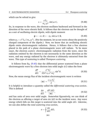
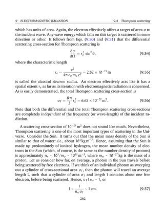
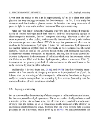
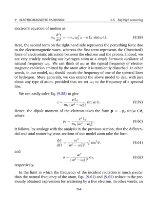
![9 ELECTROMAGNETIC RADIATION 9.8 Dielectric constant of a plasma
which is indeed greater than c. However, the theory of relativity does not forbid
this. What the theory of relativity says is that information cannot travel at a
velocity greater than c. And the peaks and troughs of an infinite plane-wave,
such as (9.78), do not carry any information.
We now need to consider how we could transmit information through a plasma
(or any other dielectric medium) by means of electromagnetic waves. The easiest
way would be to send a series of short discrete wave-pulses through the plasma,
so that we could encode information in a sort of Morse code. We can build up
a wave-pulse from a suitable superposition of infinite plane-waves of different
frequencies and wave-lengths: e.g.,
Ez(x, t) = F(k) ei φ(k)
dk, (9.83)
where φ(k) = k x − ω(k) t, and ω(k) is determined from the dispersion relation
(9.81). Now, it turns out that a relatively short wave-pulse can only be built up
from a superposition of plane-waves with a relatively wide range of different k
values. Hence, for a short wave-pulse, the integrand in the above formula consists
of the product of a fairly slowly varying function, F(k), and a rapidly oscillating
function, exp[i φ(k)]. The latter function is rapidly oscillating because the phase
φ(k) varies very rapidly with k, relative to F(k). We expect the net result of inte-
grating the product of a slowly varying function and rapidly oscillating function
to be small, since the oscillations will generally average to zero. It follows that
the integral (9.83) is dominated by those regions of k-space for which φ(k) varies
least rapidly with k. Hence, the peak of the wave-pulse most likely corresponds
to a maximum or minimum of φ(k): i.e.,
dφ
dk
= x −
dω
dk
t = 0. (9.84)
Thus, we infer that the velocity of the wave-pulse (which corresponds to the
velocity of the peak) is given by
vg =
dω
dk
. (9.85)
This velocity is called the group velocity, and is different to the phase velocity
in dispersive media, for which ω is not directly proportional to k. (Of course,
270](https://image.slidesharecdn.com/fitzpatrick-140618223522-phpapp01/85/Fitzpatrick-r-classical-electromagnetism-270-320.jpg)
![9 ELECTROMAGNETIC RADIATION 9.9 Faraday rotation
respectively. In the limit ω ωp, Ω, we obtain
k± k ± ∆k, (9.104)
where k = ω [1 − (1/2) ω2
p/ω2
]/c and ∆k = (1/2) (ω2
p/ω2
) Ω/c. In other words,
in a magnetized plasma, right- and left-hand circularly polarized waves of the
same frequency have slightly different wave-numbers
Let us now consider the propagation of a linearly polarized electromagnetic
wave through the plasma. Such a wave can be constructed via a superposition of
right- and left-hand circularly polarized waves of equal amplitudes. So, the wave
electric field can be written
E = E0 ei (k+ z−ω t)
e+ + ei (k− z−ω t)
e− . (9.105)
It can easily be seen that at z = 0 the wave electric field is aligned along the x-
axis. If right- and left-hand circularly polarized waves of the same frequency have
the same wave-number (i.e., if k+ = k−) then the wave electric field will continue
to be aligned along the x-axis as the wave propagates in the +z-direction: i.e.,
we will have a standard linearly polarized wave. However, we have just demon-
strated that, in the presence of a longitudinal magnetic field, the wave-numbers
k+ and k− are slightly different. What effect does this have on the polarization of
the wave?
Taking the real part of Eq. (9.105), and making use of Eq. (9.104), and some
standard trigonometrical identities, we obtain
E = E0 [cos(k z − ω t) cos(∆k z), cos(k z − ω t) sin(∆k z), 0] . (9.106)
The polarization angle of the wave (which is a convenient measure of its plane
of polarization) is given by
ϕ = tan−1
(Ey/Ex) = ∆k z. (9.107)
Thus, we conclude that in the presence of a longitudinal magnetic field the polar-
ization angle rotates as as the wave propagates through the plasma. This effect is
known as Faraday rotation. It is clear, from the above expression, that the rate of
advance of the polarization angle with distance travelled by the wave is given by
dϕ
dz
= ∆k =
ω2
p Ω
2 ω2 c
=
e3
2 0 m2
e c
ne B0
ω2
. (9.108)
275](https://image.slidesharecdn.com/fitzpatrick-140618223522-phpapp01/85/Fitzpatrick-r-classical-electromagnetism-275-320.jpg)
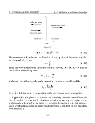
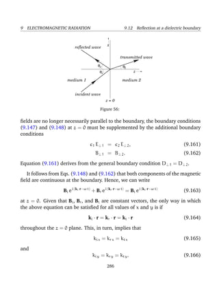
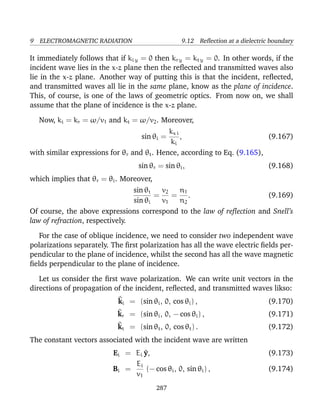
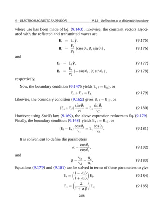
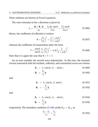
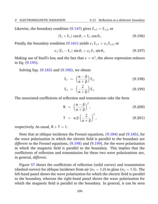
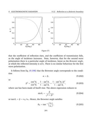
![10 RELATIVITY AND ELECTROMAGNETISM 10.3 The Lorentz transformation
observer in S will find that
dx2
+ dy2
+ dz2
− c2
dt2
= 0 (10.6)
for dt > 0, and an observer in S will find that
dx 2
+ dy 2
+ dz 2
− c2
dt 2
= 0 (10.7)
for dt > 0. Any event near P whose coordinates satisfy either (10.6) or (10.7) is
illuminated by the flash from P, and, therefore, its coordinates must satisfy both
(10.6) and (10.7). Now, no matter what form the transformation between coor-
dinates in the two inertial frames takes, the transformation between differentials
at any fixed event P is linear and homogeneous. In other words, if
x = F(x, y, z, t), (10.8)
where F is a general function, then
dx =
∂F
∂x
dx +
∂F
∂y
dy +
∂F
∂z
dz +
∂F
∂t
dt. (10.9)
It follows that
dx 2
+ dy 2
+ dz 2
− c2
dt 2
= a dx2
+ b dy2
+ c dz2
+ d dt2
+ g dx dt + h dy dt
+k dz dt + l dy dz + m dx dz + n dx dy, (10.10)
where a, b, c, etc. are functions of x, y, z, and t. We know that the right-hand
side of the above expression vanishes for all real values of the differentials which
satisfy Eq. (10.6). It follows that the right-hand side is a multiple of the quadratic
in Eq. (10.6): i.e.,
dx 2
+ dy 2
+ dz 2
− c2
dt 2
= K (dx2
+ dy2
+ dz2
− c2
dt2
), (10.11)
where K is a function of x, y, z, and t. [We can prove this by substituting into
Eq. (10.10) the following obvious zeros of the quadratic in Eq. (10.6): (±1, 0, 0, 1),
(0, ±1, 0, 1), (0, 0, ±1, 1), (0, 1/
√
2, 1/
√
2, 1), (1/
√
2, 0, 1/
√
2, 1), (1/
√
2, 1/
√
2, 0, 1):
and solving the resulting conditions on the coefficients.] Note that K at P is also
independent of the choice of standard coordinates in S and S . Since the frames
are Euclidian, the values of dx2
+ dy2
+ dz2
and dx 2
+ dy 2
+ dz 2
relevant to P
301](https://image.slidesharecdn.com/fitzpatrick-140618223522-phpapp01/85/Fitzpatrick-r-classical-electromagnetism-301-320.jpg)
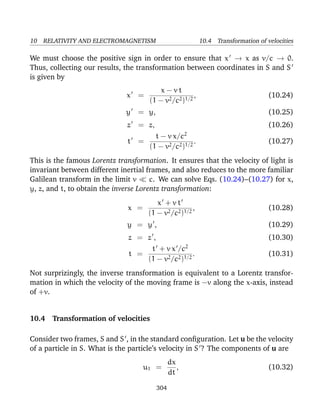
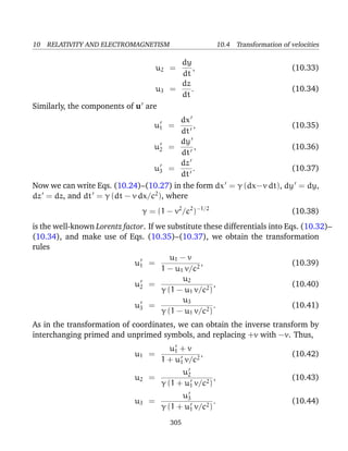
![10 RELATIVITY AND ELECTROMAGNETISM 10.4 Transformation of velocities
Equations (10.42)–(10.44) can be regarded as giving the resultant, u = (u1, u2, u3),
of two velocities, v = (v, 0, 0) and u = (u1, u2, u3), and are therefore usually
referred to as the relativistic velocity addition formulae. The following relation
between the magnitudes u = (u 2
1 + u 2
2 + u 2
3 )1/2
and u = (u1
2
+ u2
2
+ u3
2
)1/2
of
the velocities is easily demonstrated:
c2
− u2
=
c2
(c2
− u 2
) (c2
− v2
)
(c2 + u1 v)2
. (10.45)
If u < c and v < c then the right-hand side is positive, implying that u < c.
In other words, the resultant of two subluminal velocities is another subluminal
velocity. It is evident that a particle can never attain the velocity of light relative
to a given inertial frame, no matter how many subluminal velocity increments it
is given. It follows that no inertial frame can ever appear to propagate with a
superluminal velocity with respect to any other inertial frame (since we can track
a given inertial frame using a particle which remains at rest at the origin of that
frame).
According to Eq. (10.45), if u = c then u = c, no matter what value v takes:
i.e., the velocity of light is invariant between different inertial frames. Note that
the Lorentz transform only allows one such invariant velocity [i.e., the velocity
c which appears in Eqs. (10.24)–(10.27)]. Einstein’s relativity principle tells us
that any disturbance which propagates through a vacuum must appear to prop-
agate at the same velocity in all inertial frames. It is now evident that all such
disturbances must propagate at the velocity c. It follows immediately that all
electromagnetic waves must propagate through the vacuum with this velocity,
irrespective of their wavelength. In other words, it is impossible for there to be
any dispersion of electromagnetic waves propagating through a vacuum. Fur-
thermore, gravity waves must also propagate with the velocity c.
The Lorentz transformation implies that the velocities of propagation of all
physical effects are limited by c in deterministic physics. Consider a general
process by which an event P causes an event Q at a velocity U > c in some frame
S. In other words, information about the event P appears to propagate to the
event Q with a superluminal velocity. Let us choose coordinates such that these
two events occur on the x-axis with (finite) time and distance separations ∆t > 0
306](https://image.slidesharecdn.com/fitzpatrick-140618223522-phpapp01/85/Fitzpatrick-r-classical-electromagnetism-306-320.jpg)
![10 RELATIVITY AND ELECTROMAGNETISM 10.5 Tensors
and ∆x > 0, respectively. The time separation in some other inertial frame S is
given by [see Eq. (10.27)]
∆t = γ (∆t − v ∆x/c2
) = γ ∆t (1 − v U/c2
). (10.46)
Thus, for sufficiently large v < c we obtain ∆t < 0: i.e., there exist inertial frames
in which cause and effect appear to be reversed. Of course, this is impossible in
deterministic physics. It follows, therefore, that information can never appear to
propagate with a superluminal velocity in any inertial frame, otherwise causality
would be violated.
10.5 Tensors
It is now convenient to briefly review the mathematics of tensors. Tensors are
of primary importance in connection with coordinate transforms. They serve to
isolate intrinsic geometric and physical properties from those that merely depend
on coordinates.
A tensor of rank r in an n-dimensional space possesses nr
components which
are, in general, functions of position in that space. A tensor of rank zero has one
component, A, and is called a scalar. A tensor of rank one has n components,
(A1, A2, · · · , An), and is called a vector. A tensor of rank two has n2
components,
which can be exhibited in matrix format. Unfortunately, there is no convenient
way of exhibiting a higher rank tensor. Consequently, tensors are usually repre-
sented by a typical component: e.g., the tensor Aijk (rank 3), or the tensor Aijkl
(rank 4), etc. The suffixes i, j, k, · · · are always understood to range from 1 to n.
For reasons which will become apparent later on, we shall represent tensor
components using both superscripts and subscripts. Thus, a typical tensor might
look like Aij
(rank 2), or Bi
j (rank 2), etc. It is convenient to adopt the Einstein
summation convention. Namely, if any suffix appears twice in a given term, once
as a subscript and once as a superscript, a summation over that suffix (from 1 to
n) is implied.
To distinguish between various different coordinate systems, we shall use primed
and multiply primed suffixes. A first system of coordinates (x1
, x2
, · · · , xn
) can
307](https://image.slidesharecdn.com/fitzpatrick-140618223522-phpapp01/85/Fitzpatrick-r-classical-electromagnetism-307-320.jpg)
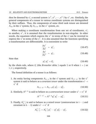
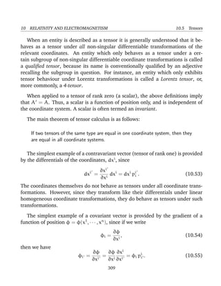
![10 RELATIVITY AND ELECTROMAGNETISM 10.8 Proper time
It is clear that dt = dτ in the particle’s rest frame. Thus, dτ corresponds to the
time difference between two neighbouring events on the particle’s world-line,
as measured by a clock attached to the particle (hence, the name proper time).
According to Eq. (10.100), the particle’s clock appears to run slow, by a factor
γ(u), in an inertial frame in which the particle is moving with velocity u. This is
the celebrated time dilation effect.
Let us consider how a small 4-dimensional volume element in space-time
transforms under a general Lorentz transformation. We have
d4
x = J d4
x, (10.101)
where
J =
∂(x1
, x2
, x3
, x4
)
∂(x1, x2, x3, x4)
(10.102)
is the Jacobian of the transformation: i.e., the determinant of the transformation
matrix pµ
µ . A general Lorentz transformation is made up of a standard Lorentz
transformation plus a displacement and a rotation. Thus, the transformation ma-
trix is the product of that for a standard Lorentz transformation, a translation,
and a rotation. It follows that the Jacobian of a general Lorentz transformation
is the product of that for a standard Lorentz transformation, a translation, and a
rotation. It is well-known that the Jacobian of the latter two transformations is
unity, since they are both volume preserving transformations which do not affect
time. Likewise, it is easily seen [e.g., by taking the determinant of the transfor-
mation matrix (10.79)] that the Jacobian of a standard Lorentz transformation is
also unity. It follows that
d4
x = d4
x (10.103)
for a general Lorentz transformation. In other words, a general Lorentz transfor-
mation preserves the volume of space-time. Since time is dilated by a factor γ in
a moving frame, the volume of space-time can only be preserved if the volume of
ordinary 3-space is reduced by the same factor. As is well-known, this is achieved
by length contraction along the direction of motion by a factor γ.
320](https://image.slidesharecdn.com/fitzpatrick-140618223522-phpapp01/85/Fitzpatrick-r-classical-electromagnetism-320-320.jpg)
![10 RELATIVITY AND ELECTROMAGNETISM 10.9 4-velocity and 4-acceleration
10.9 4-velocity and 4-acceleration
We have seen that the quantity dxµ
/ds transforms as a 4-vector under a general
Lorentz transformation [see Eq. (10.67)]. Since ds ∝ dτ it follows that
Uµ
=
dxµ
dτ
(10.104)
also transforms as a 4-vector. This quantity is known as the 4-velocity. Likewise,
the quantity
Aµ
=
d2
xµ
dτ2
=
dUµ
dτ
(10.105)
is a 4-vector, and is called the 4-acceleration.
For events along the world-line of a particle traveling with 3-velocity u, we
have
Uµ
=
dxµ
dτ
=
dxµ
dt
dt
dτ
= γ(u) (u, c), (10.106)
where use has been made of Eq. (10.100). This gives the relationship between a
particle’s 3-velocity and its 4-velocity. The relationship between the 3-acceleration
and the 4-acceleration is less straightforward. We have
Aµ
=
dUµ
dτ
= γ
dUµ
dt
= γ
d
dt
(γ u, γ c) = γ
dγ
dt
u + γ a, c
dγ
dt
, (10.107)
where a = du/dt is the 3-acceleration. In the rest frame of the particle, Uµ
=
(0, c) and Aµ
= (a, 0). It follows that
UµAµ
= 0 (10.108)
(note that UµAµ
is an invariant quantity). In other words, the 4-acceleration of a
particle is always orthogonal to its 4-velocity.
10.10 The current density 4-vector
Let us now consider the laws of electromagnetism. We wish to demonstrate that
these laws are compatible with the relativity principle. In order to achieve this, it
321](https://image.slidesharecdn.com/fitzpatrick-140618223522-phpapp01/85/Fitzpatrick-r-classical-electromagnetism-321-320.jpg)
![10 RELATIVITY AND ELECTROMAGNETISM 10.13 Retarded potentials
Note that even after the Lorentz gauge has been adopted, the potentials are un-
determined to a gauge transformation using a scalar field, ψ, which satisfies the
sourceless wave equation
2ψ = 0. (10.128)
However, if we adopt sensible boundary conditions in both space and time then
the only solution to the above equation is ψ = 0.
10.13 Retarded potentials
We already know the solutions to Eqs. (10.117) and (10.118). They take the
form (see Sect. 4.9)
φ(r, t) =
1
4π 0
[ρ(r )]
|r − r |
dV , (10.129)
A(r, t) =
µ0
4π
[j(r )]
|r − r |
dV . (10.130)
The above equations can be combined to form the solution of the 4-vector wave
equation (10.120),
Φµ
=
1
4π 0 c
[Jµ
]
r
dV. (10.131)
Here, the components of the 4-potential are evaluated at some event P in space-
time, r is the distance of the volume element dV from P, and the square brackets
indicate that the 4-current is to be evaluated at the retarded time: i.e., at a time
r/c before P.
But, does the right-hand side of Eq. (10.131) really transform as a contravari-
ant 4-vector? This is not a trivial question, since volume integrals in 3-space are
not, in general, Lorentz invariant due to the length contraction effect. However,
the integral in Eq. (10.131) is not a straightforward volume integral, because the
integrand is evaluated at the retarded time. In fact, the integral is best regarded
as an integral over events in space-time. The events which enter the integral
are those which intersect a spherical light wave launched from the event P and
evolved backwards in time. In other words, the events occur before the event P,
325](https://image.slidesharecdn.com/fitzpatrick-140618223522-phpapp01/85/Fitzpatrick-r-classical-electromagnetism-325-320.jpg)
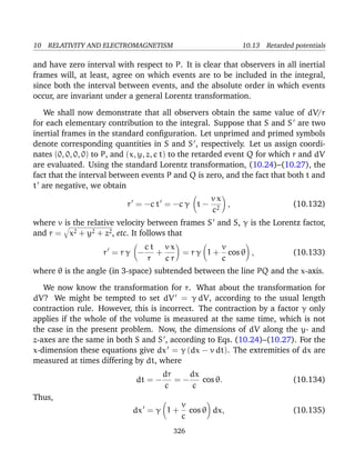
![10 RELATIVITY AND ELECTROMAGNETISM 10.14 Tensors and pseudo-tensors
giving
dV = γ 1 +
v
c
cos θ dV. (10.136)
It follows from Eqs. (10.133) and (10.136) that dV /r = dV/r. This result will
clearly remain valid even when S and S are not in the standard configuration.
Thus, dV/r is an invariant and, therefore, [Jµ
] dV/r is a contravariant 4-vector.
For linear transformations, such as a general Lorentz transformation, the result
of adding 4-tensors evaluated at different 4-points is itself a 4-tensor. It follows
that the right-hand side of Eq. (10.131) is indeed a contravariant 4-vector. Thus,
this 4-vector equation can be properly regarded as the solution to the 4-vector
wave equation (10.120).
10.14 Tensors and pseudo-tensors
The totally antisymmetric fourth rank tensor is defined
αβγδ
=
+1 for α, β, γ, δ any even permutation of 1, 2, 3, 4
−1 for α, β, γ, δ any odd permutation of 1, 2, 3, 4
0 otherwise
(10.137)
The components of this tensor are invariant under a general Lorentz transforma-
tion, since
αβγδ
pα
α pβ
β pγ
γ pδ
δ = α β γ δ
|pµ
µ | = α β γ δ
, (10.138)
where |pµ
µ | denotes the determinant of the transformation matrix, or the Jacobian
of the transformation, which we have already established is unity for a general
Lorentz transformation. We can also define a totally antisymmetric third rank
tensor ijk
which stands in the same relation to 3-space as αβγδ
does to space-
time. It is easily demonstrated that the elements of ijk
are invariant under a
general translation or rotation of the coordinate axes. The totally antisymmetric
third rank tensor is used to define the cross product of two 3-vectors,
(a × b)i
= ijk
aj bk, (10.139)
327](https://image.slidesharecdn.com/fitzpatrick-140618223522-phpapp01/85/Fitzpatrick-r-classical-electromagnetism-327-320.jpg)
![10 RELATIVITY AND ELECTROMAGNETISM 10.18 Potential due to a moving charge
is (permanently) at rest at (say) the point (x , y , z ). In S , the potential at P is
the usual potential due to a stationary charge,
A = 0, (10.196)
φ =
e
4π 0 r
, (10.197)
where r = x 2 + y 2 + z 2. Let us now transform these equations directly into
the frame S. Since Aµ
= (c A, φ) is a contravariant 4-vector, its components
transform according to the standard rules (10.75)–(10.78). Thus,
c A1 = γ c A1 +
u
c
φ =
γ u e
4π 0 c r
, (10.198)
c A2 = c A2 = 0, (10.199)
c A3 = c A3 = 0, (10.200)
φ = γ φ +
u
c
c A1 =
γ e
4π 0 r
, (10.201)
since β = −u/c in this case. It remains to express the quantity r in terms of
quantities measured in S. The most physically meaningful way of doing this is
to express r in terms of retarded values in S. Consider the retarded event at the
charge for which, by definition, r = −c t and r = −c t. Using the standard
Lorentz transformation, (10.24)–(10.27), we find that
r = −c t = −c γ (t − u x/c2
) = r γ (1 + ur/c), (10.202)
where ur = u x/r = r·u/r denotes the radial velocity of the change in S. We can
now rewrite Eqs. (10.198)–(10.201) in the form
A =
µ0 e
4π
[u]
[r + r·u/c]
, (10.203)
φ =
e
4π 0
1
[r + r·u/c]
, (10.204)
where the square brackets, as usual, indicate that the enclosed quantities must
be retarded. For a uniformly moving charge, the retardation of u is, of course,
superfluous. However, since
Φµ
=
1
4π 0 c
[Jµ
]
r
dV, (10.205)
338](https://image.slidesharecdn.com/fitzpatrick-140618223522-phpapp01/85/Fitzpatrick-r-classical-electromagnetism-338-320.jpg)
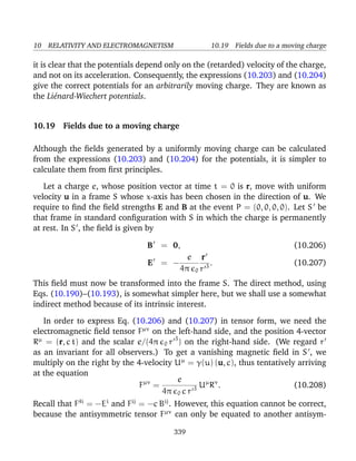
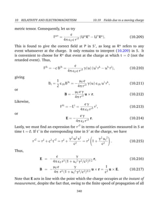
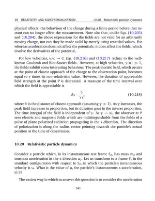
![10 RELATIVITY AND ELECTROMAGNETISM 10.20 Relativistic particle dynamics
4-vector [see Eq. (10.107)]
Aµ
= γ
dγ
dt
u + γ a, c
dγ
dt
. (10.219)
Using the standard transformation, (10.75)–(10.78), for 4-vectors, we obtain
a0 = γ3
a, (10.220)
dγ
dt
=
u a0
c2
. (10.221)
Equation (10.220) can be written
f = m0 γ3 du
dt
, (10.222)
where f = m0 a0 is the constant force (in the x-direction) acting on the particle
in S0.
Equation (10.222) is equivalent to
f =
d(m u)
dt
, (10.223)
where
m = γ m0. (10.224)
Thus, we can account for the ever decreasing acceleration of a particle subject
to a constant force [see Eq. (10.220)] by supposing that the inertial mass of the
particle increases with its velocity according to the rule (10.224). Henceforth,
m0 is termed the rest mass, and m the inertial mass.
The rate of increase of the particle’s energy E satisfies
dE
dt
= f u = m0 γ3
u
du
dt
. (10.225)
This equation can be written
dE
dt
=
d(m c2
)
dt
, (10.226)
342](https://image.slidesharecdn.com/fitzpatrick-140618223522-phpapp01/85/Fitzpatrick-r-classical-electromagnetism-342-320.jpg)
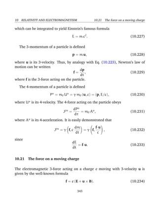
![10 RELATIVITY AND ELECTROMAGNETISM 10.22 The electromagnetic energy tensor
where Fµν
is the electromagnetic field tensor, and Gµν
is its dual. As is easily
verified, Eq. (10.249) can also be written in the form
∂µFνσ + ∂νFσµ + ∂σFµν = 0. (10.250)
Equations (10.246) and (10.248) can be combined to give
fν = 0 Fνσ ∂µFµσ
. (10.251)
This expression can also be written
fν = 0 [∂µ(Fµσ
Fνσ) − Fµσ
∂µFνσ] . (10.252)
Now,
Fµσ
∂µFνσ =
1
2
Fµσ
(∂µFνσ + ∂σFµν), (10.253)
where use has been made of the antisymmetry of the electromagnetic field tensor.
It follows from Eq. (10.250) that
Fµσ
∂µFνσ = −
1
2
Fµσ
∂νFσµ =
1
4
∂ν(Fµσ
Fµσ). (10.254)
Thus,
fν = 0 ∂µ(Fµσ
Fνσ) −
1
4
∂ν(Fµσ
Fµσ) . (10.255)
The above expression can also be written
fν = −∂µTµ
ν, (10.256)
where
Tµ
ν = 0 Fµσ
Fσν +
1
4
δµ
ν (Fρσ
Fρσ) (10.257)
is called the electromagnetic energy tensor. Note that Tµ
ν is a proper-4-tensor. It
follows from Eqs. (10.159), (10.162), and (10.194) that
Ti
j = 0 Ei
Ej +
Bi
Bj
µ0
− δi
j
1
2
0 Ek
Ek +
Bk
Bk
µ0
, (10.258)
Ti
4 = −T4
i =
ijk
EjBk
µ0 c
, (10.259)
T4
4 =
1
2
0 Ek
Ek +
Bk
Bk
µ0
. (10.260)
346](https://image.slidesharecdn.com/fitzpatrick-140618223522-phpapp01/85/Fitzpatrick-r-classical-electromagnetism-346-320.jpg)
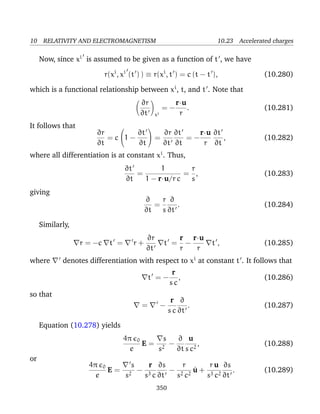
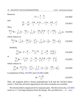
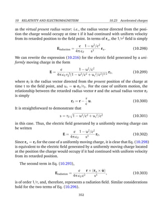
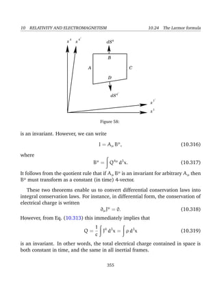
![10 RELATIVITY AND ELECTROMAGNETISM 10.25 Radiation losses
Thus, in a linear accelerator, the radiated power depends on the external force
acting on the particle, and not on the actual energy or momentum of the particle.
It is obvious, from the above formula, that light particles, such as electrons, are
going to radiate a lot more than heavier particles, such as protons. The ratio of
the power radiated to the power supplied by the external sources is
P
dE/dt
=
e2
6π 0 m2
0 c3
1
u
dE
dx
e2
6π 0 m0 c2
1
m0 c2
dE
dx
, (10.331)
since u c for a highly relativistic particle. It is clear, from the above ex-
pression, that the radiation losses in an electron linear accelerator are negligi-
ble unless the gain in energy is of order me c2
= 0.511 MeV in a distance of
e2
/(6π 0 me c2
) = 1.28 × 10⁻¹⁵
meters. That is 3 × 10¹⁴
MeV/meter. Typical
energy gains are less that 10 MeV/meter. It follows, therefore, that radiation
losses are completely negligible in linear accelerators, whether for electrons, or
for other heavier particles.
The situation is quite different in circular accelerator devices, such as the syn-
chrotron and the betatron. In such machines, the momentum p changes rapidly
in direction as the particle rotates, but the change in energy per revolution is
small. Furthermore, the direction of acceleration is always perpendicular to the
direction of motion. It follows from Eq. (10.327) that
P =
e2
6π 0 c3
γ4
˙u2
=
e2
6π 0 c3
γ4
u4
ρ2
, (10.332)
where ρ is the orbit radius. Here, use has been made of the standard result
˙u = u2
/ρ for circular motion. The radiative energy loss per revolution is given by
δE =
2π ρ
u
P =
e2
3 0 c3
γ4
u3
ρ
. (10.333)
For highly relativistic (u c) electrons, this expression yields
δE(MeV) = 8.85 × 10⁻² [E(GeV)]4
ρ(meters)
. (10.334)
In the first electron synchrotrons, ρ ∼ 1 meter, Emax ∼ 0.3 GeV. Hence, δEmax ∼ 1
keV per revolution. This was less than, but not negligible compared to, the en-
ergy gain of a few keV per turn. For modern electron synchrotrons, the limitation
358](https://image.slidesharecdn.com/fitzpatrick-140618223522-phpapp01/85/Fitzpatrick-r-classical-electromagnetism-358-320.jpg)
![10 RELATIVITY AND ELECTROMAGNETISM 10.26 Angular distribution of radiation
on the available radio-frequency power needed to overcome radiation losses be-
comes a major consideration, as is clear from the E4
dependence of the radiated
power per turn.
10.26 Angular distribution of radiation
In order to calculate the angular distribution of the energy radiated by an acceler-
ated charge, we must think carefully about what is meant by the rate of radiation
of the charge. This quantity is actually the amount of energy lost by the charge
in a retarded time interval dt during the emission of the signal. Thus,
P(t ) = −
dE
dt
, (10.335)
where E is the energy of the charge. The Poynting vector
Erad × Brad
µ0
= 0 c E2
rad
r
r
, (10.336)
where use has been made of Brad = (r × Erad)/r c [see Eq. (10.297)], represents
the energy flux per unit actual time, t. Thus, the energy loss rate of the charge
into a given element of solid angle dΩ is
dP(t )
dΩ
dΩ = −
dE(θ, ϕ)
dt
dΩ =
dE(θ, ϕ)
dt
dt
dt
r2
dΩ = 0 c E2
rad
s
r
r2
dΩ, (10.337)
where use has been made of Eq. (10.283). Here, θ and ϕ are angular coordinates
used to locate the element of solid angle. It follows from Eq. (10.303) that
dP(t )
dΩ
=
e2
r
16π2
0 c3
[r × (ru × ˙u)]2
s5
. (10.338)
Consider the special case in which the direction of acceleration coincides with
the direction of motion. Let us define spherical polar coordinates whose axis
points along this common direction. It is easily demonstrated that, in this case,
the above expression reduces to
dP(t )
dΩ
=
e2
˙u2
16π2
0 c3
sin2
θ
[1 − (u/c) cos θ]5
. (10.339)
359](https://image.slidesharecdn.com/fitzpatrick-140618223522-phpapp01/85/Fitzpatrick-r-classical-electromagnetism-359-320.jpg)
![10 RELATIVITY AND ELECTROMAGNETISM 10.27 Synchrotron radiation
In the non-relativistic limit, u/c → 0, the radiation pattern has the familiar sin2
θ
dependence of dipole radiation. In particular, the pattern is symmetric in the
forward (θ < π/2) and backward (θ > π/2) directions. However, as u/c → 1, the
radiation pattern becomes more and more concentrated in the forward direction.
The angle θmax for which the intensity is a maximum is
θmax = cos−1
1
3 u/c
( 1 + 15 u2/c2 − 1)
. (10.340)
This expression yields θmax → π/2 as u/c → 0, and θmax → 1/(2 γ) as u/c → 1.
Thus, for a highly relativistic charge, the radiation is emitted in a narrow cone
whose axis is aligned along the direction of motion. In this case, the angular
distribution (10.339) reduces to
dP(t )
dΩ
2 e2
˙u2
π2
0c3
γ8 (γ θ)2
[1 + (γ θ)2]5
. (10.341)
The total power radiated by the charge is obtained by integrating Eq. (10.339)
over all solid angles. We obtain
P(t ) =
e2
˙u2
8π 0 c3
π
0
sin3
θ dθ
[1 − (u/c) cos θ]5
=
e2
˙u2
8π 0 c3
+1
−1
(1 − µ2
) dµ
[1 − (u/c) µ]5
. (10.342)
It is easily verified that
+1
−1
(1 − µ2
) dµ
[1 − (u/c) µ]5
=
4
3
γ6
. (10.343)
Hence,
P(t ) =
e2
6π 0 c3
γ6
˙u2
, (10.344)
which agrees with Eq. (10.327), provided that u × ˙u = 0.
10.27 Synchrotron radiation
Synchrotron radiation (i.e., radiation emitted by a charged particle constrained
to follow a circular orbit by a magnetic field) is of particular importance in as-
trophysics, since much of the observed radio frequency emission from supernova
remnants and active galactic nuclei is thought to be of this type.
360](https://image.slidesharecdn.com/fitzpatrick-140618223522-phpapp01/85/Fitzpatrick-r-classical-electromagnetism-360-320.jpg)
![10 RELATIVITY AND ELECTROMAGNETISM 10.27 Synchrotron radiation
Consider a charged particle moving in a circle of radius a with constant angu-
lar velocity ω0. Suppose that the orbit lies in the x-y plane. The radius vector
pointing from the centre of the orbit to the retarded position of the charge is
defined
ρ = a (cos φ, sin φ, 0), (10.345)
where φ = ω0 t is the angle subtended between this vector and the x-axis. The
retarded velocity and acceleration of the charge take the form
u =
dρ
dt
= u (− sin φ, cos φ, 0), (10.346)
˙u =
du
dt
= −˙u (cos φ, sin φ, 0), (10.347)
where u = a ω0 and ˙u = a ω 2
0 . The observation point is chosen such that the ra-
dius vector r, pointing from the retarded position of the charge to the observation
point, is parallel to the y-z plane. Thus, we can write
r = r (0, sin α, cos α), (10.348)
where α is the angle subtended between this vector and the z-axis. As usual, we
define θ as the angle subtended between the retarded radius vector r and the
retarded direction of motion of the charge u. It follows that
cos θ =
u·r
u r
= sin α cos φ. (10.349)
It is easily seen that
˙u·r = −˙u r sin α sin φ. (10.350)
A little vector algebra shows that
[r × (ru × ˙u)]2
= −(r·˙u)2
r2
(1 − u2
/c2
) + ˙u2
r4
(1 − r·u/r c)2
, (10.351)
giving
[r × (ru × ˙u)]2
= ˙u2
r4
1 −
u
c
cos θ
2
−
1 −
u2
c2
tan2
φ cos2
θ
. (10.352)
361](https://image.slidesharecdn.com/fitzpatrick-140618223522-phpapp01/85/Fitzpatrick-r-classical-electromagnetism-361-320.jpg)
![10 RELATIVITY AND ELECTROMAGNETISM 10.27 Synchrotron radiation
Making use of Eq. (10.337), we obtain
dP(t )
dΩ
=
e2
˙u2
16π2
0 c3
[1 − (u/c) cos θ)]2
− (1 − u2
/c2
) tan2
φ cos2
θ
[1 − (u/c) cos θ]5
. (10.353)
It is convenient to write this result in terms of the angles α and φ, instead of θ
and φ. After a little algebra we obtain
dP(t )
dΩ
=
e2
˙u2
16π2
0 c3
[1 − (u2
/c2
)] cos2
α + [(u/c) − sin α cos φ]2
[1 − (u/c) sin α cos φ]5
. (10.354)
Let us consider the radiation pattern emitted in the plane of the orbit: i.e.,
α = π/2, with cos φ = cos θ . It is easily seen that
dP(t )
dΩ
=
e2
˙u2
16π2
0 c3
[(u/c) − cos θ]2
[1 − (u/c) cos θ]5
. (10.355)
In the non-relativistic limit, the radiation pattern has a cos2
θ dependence. Thus,
the pattern is like that of dipole radiation where the axis is aligned along the
instantaneous direction of acceleration. As the charge becomes more relativistic,
the radiation lobe in the forward direction (i.e., 0 < θ < π/2) becomes more
more focused and more intense. Likewise, the radiation lobe in the backward
direction (i.e., π/2 < θ < π) becomes more diffuse. The radiation pattern has
zero intensity at the angles
θ0 = cos−1
(u/c). (10.356)
These angles demark the boundaries between the two radiation lobes. In the
non-relativistic limit, θ0 = ±π/2, so the two lobes are of equal angular extents.
In the highly relativistic limit, θ0 → ±1/γ, so the forward lobe becomes highly
concentrated about the forward direction (θ = 0). In the latter limit, Eq. (10.355)
reduces to
dP(t )
dΩ
e2
˙u2
2π2
0 c3
γ6 [1 − (γ θ)2
]2
[1 + (γ θ)2]5
. (10.357)
Thus, the radiation emitted by a highly relativistic charge is focused into an in-
tense beam, of angular extent 1/γ, pointing in the instantaneous direction of
motion. The maximum intensity of the beam scales like γ6
.
362](https://image.slidesharecdn.com/fitzpatrick-140618223522-phpapp01/85/Fitzpatrick-r-classical-electromagnetism-362-320.jpg)

This document is the contents page and introduction to an intermediate level course on classical electromagnetism taught by Richard Fitzpatrick at the University of Texas at Austin. The course covers topics such as vector algebra, Maxwell's equations, electrostatics, magnetic induction, electromagnetic energy and momentum, electromagnetic radiation, and relativity and electromagnetism. It is divided into 10 chapters that progress from basic vector concepts to more advanced topics involving dielectrics, radiation, and relativity.