This document is a dissertation presented by Alexandre Colmant for the degree of Doctor of Philosophy in engineering at Stellenbosch University. It presents a generic decision support system (DSS) designed to assist operators in maritime law enforcement (MLE) response selection and resource routing decisions.
The DSS uses kinematic vessel data from threat detection and evaluation systems as well as subjective operator input to make semi-automated decisions about dispatching MLE resources like patrol vessels, military vessels, and helicopters. The goal is to employ resources effectively and efficiently rather than fully automate decision making.
The DSS accommodates multiple response selection objectives in a generic manner so users can configure their own goals. Models capable of the DSS


![CHAPTER 1
Introduction
Contents
1.1 Background . . . . . . . . . . . . . . . . . . . . . . . . . . . . . . . . . . . . . . 1
1.1.1 The law of the seas . . . . . . . . . . . . . . . . . . . . . . . . . . . . . . 2
1.1.2 Activities of vessels at sea . . . . . . . . . . . . . . . . . . . . . . . . . . 2
1.2 Informal problem description . . . . . . . . . . . . . . . . . . . . . . . . . . . . 4
1.3 Dissertation aim and scope . . . . . . . . . . . . . . . . . . . . . . . . . . . . . 9
1.4 Dissertation objectives . . . . . . . . . . . . . . . . . . . . . . . . . . . . . . . . 9
1.5 Dissertation organisation . . . . . . . . . . . . . . . . . . . . . . . . . . . . . . . 11
Following the raid of an al-Qa’ida intelligence base in May 2011, evidence was uncovered suggest-
ing that the terrorist organisation planned to blow up an unknown number of oil tankers within
the US maritime transportation system [146]. Due to the strengths of their hulls, these tankers
either have to be blown up from the inside (as the result of an inside-job) or, more likely, have to
be intercepted by a terrorist vessel while in transit (and then blown up). The large quantity of
tankers transiting these waters, combined with the vastness of the US maritime transportation
system and the limited security resources available, however, has made it impossible for the US
maritime defense authorities to achieve constant coverage of potentially threatening activities
occurring in the vicinity of these terrorist targets. In addition, it was believed that the adversary
had had the opportunity to observe security patrol patterns in order to better plan its attacking
strategy. This alarming situation, coupled with challenging economic times, has forced the US
maritime defense authorities to deploy its resources as effectively as possible so as to minimise
the risk of allowing potentially threatening activities to progress towards the destruction of one
or more targets, while simultaneously attempting to maintain operating costs at a minimum
level [148].
1.1 Background
The obligations and privileges of coastal nations form part of a global legislation process to
create an efficient international framework defining their rights and responsibilities in respect of
seabeds and ocean floors. The establishment of such a framework is, however, a very complex
process, and has for centuries been a frustrating and unfulfilled idealistic notion [151]. It is
instructive to review certain laws pertaining to activities at sea in order to establish a context
for the complex challenges faced by coastal nations.
1](https://image.slidesharecdn.com/6cd1ebf5-5cfe-4d40-998c-99cbe17b08f1-170109122537/85/PhD-dissertation-33-320.jpg)
![2 Chapter 1. Introduction
1.1.1 The law of the seas
In 1982, the United Nations Convention on the Law of the Sea (UNCLOS) at last settled on
a legal order for the seas and oceans with the aim of promoting international communication,
peaceful uses of the seas, equitable and efficient utilisation of maritime resources, jurisdiction
demarcation over waters, and conservation of maritime ecosystems [49, 124, 151]. In addition,
this order clearly defines the nature of crimes committed at sea and provides coastal nations
with the appropriate responses to enforce a variety of laws aimed at curbing these crimes. Under
the UNCLOS, every coastal nation is given the rights and responsibilities to establish territorial
waters over which they exercise various controls, as follows:
• The outer limit of the territorial sea of a coastal nation is the line consisting of every point
at a distance of twelve nautical miles from the nearest point along the coastline [151].
The standard baseline for measuring the width of the territorial sea is the low-water line
along the coast, as marked on large-scale maps officially recognized by the coastal nation1.
Within this territory, the coastal state may exercise all sovereign rights over the seabed,
water and associated airspace, but is obliged to afford the right of innocent passage to
vessels of any state.
• The waters contiguous to the territorial sea, known as the contiguous zone, extends for
twenty four nautical miles from the same baseline from which the extent of the territorial
sea is measured. Here, the coastal state may exercise the rights to prevent violations of
its fiscal, customs, immigration and waste disposal laws [151]. Additionally, the coastal
state may also take actions within this zone to punish violations of these laws previously
committed within its land territory or territorial sea.
• The exclusive economic zone (EEZ) stretches out to sea for a further 188 miles from
the seaward boundary of the territorial sea. Here, the coastal state has the sovereign
rights to explore, exploit, conserve and manage living and nonliving natural resources; to
establish and use artificial islands, installations, and structures; to conduct marine scientific
research; and to protect and preserve the marine environment [151]. The UNCLOS is,
however, in the process of allowing certain coastal nations to extend specific zones within
their EEZ beyond 200 nautical miles from the low-water line along the coast, based on
certain physical characteristics of the continental shelf [124].
Lastly, the waters beyond the EEZ (which are not considered archipelagic waters) are defined as
the high seas. The sense of liberty enjoyed by seafarers in these waters is applicable to all states,
whether coastal or not. Subject to certain rules and regulations laid down by the UNCLOS and
other entities, navigators of the high seas have the right to freedom of navigation; the freedom
to lay underwater infrastructure; the freedom to construct artificial islands, installations and
structures; the freedom of fishing; and the freedom to perform scientific research [151]. It is,
nevertheless, imperative that these waters remain crime-free and that activities in these regions
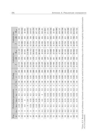
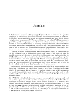
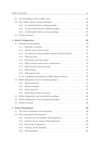
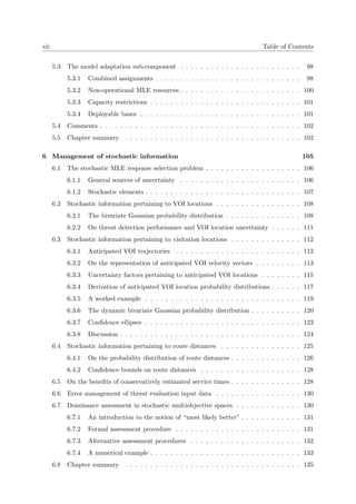
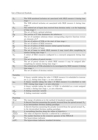
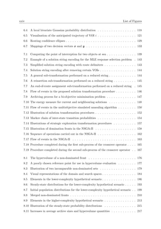
are only aimed toward peaceful ends. The four general maritime zones described above are
illustrated in Figure 1.1.
1.1.2 Activities of vessels at sea
Maritime activities by seafearing vessels embody a very important part of global society; the
globally connected economy relies on the seas and adjoined littorals for fishing, access to natural
1
In the case of islands situated on atolls or of islands having fringing reefs, the baseline for measuring the
extent of the territorial sea is the seaward low-water line of the reef.](https://image.slidesharecdn.com/6cd1ebf5-5cfe-4d40-998c-99cbe17b08f1-170109122537/85/PhD-dissertation-34-320.jpg)
![1.1. Background 3
Land
Sea
Territorial sea
(12 nm)
Contiguous zone
(12 nm)
EEZ
(188 nm)
High seas
Baseline
Figure 1.1: The four maritime zones defined by the UNCLOS [151].
resources and the transportation of most of the world’s import and export commodities. These
maritime activities today contribute, inter alia, to over 90 percent of global trade [8] and are
directly responsible for 91 million tons of food for human consumption annually [39]. Effective
governance of these maritime regions is therefore essential for both the economic growth and the
national security of coastal nations. Indeed, according to the Maritime Security Sector Reform
[124], “the maritime sector is fundamental, directly or indirectly, to the national defense, law
enforcement, social, and economic goals and objectives of nearly every country. It is a crucial
source of livelihood for many in developing nations, a platform for trade, and a theater for
potential conflict or crime.”
A sizable portion of maritime activities are unfortunately responsible for a wide variety of
problems, ranging from being detrimental to only a few individuals to harming society on a global
scale. These maritime problems are typically caused by lawless vessels that choose to disrupt the
harmony at sea for personal gain. Such activities, or threats, typically include piracy acts, illegal
or unregulated fishing, narcotics trafficking, illegal immigration, environmental degradation,
human trafficking, proliferation of weapons of mass destruction, and terrorism.
For instance, it is estimated that five to fifteen percent of all large vessels (that is, 5 000 to
7 500 vessels) break the law each year by discharging waste into the high seas, including 70 to
210 million gallons of illegal oil waste disposal [92]. Such negligence and inconsideration can
potentially devastate the marine environment on a local or even global scale. It is also estimated
that a third of all fish populations are over-exploited or have collapsed because of illegal fishing
[39]. As a result, some of these species face a constant danger of extinction, and over-exploitation
is estimated to generate an indirect annual cost of US $50 billion in lost fishing opportunities
[111], which accounts for approximately half of the value of the global seafood trade. Moreover,
the global economic cost resulting from acts of piracy is estimated to lie between US $7 and
US $12 billion per annum [10].](https://image.slidesharecdn.com/6cd1ebf5-5cfe-4d40-998c-99cbe17b08f1-170109122537/85/PhD-dissertation-35-320.jpg)
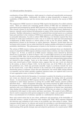
![4 Chapter 1. Introduction
1.2 Informal problem description
Pursuing the goal of effective Maritime Law Enforcement (MLE) requires coastal nations to
establish suitable monitoring procedures aimed at vessels within their jurisdictions. These pro-
cedures are underpinned by a so-called response selection process, where, following the detection
and evaluation of potentially threatening events involving vessels of interest (VOIs) at sea, MLE
resources, such as high-speed interception boats, military vessels, helicopters, and/or seaplanes,
are dispatched by coast guards and related authorities to intercept and investigate these threats.
MLE resources are generally either allocated for the purpose of intercepting VOIs at sea (such
resources are said to be in an active state), or are strategically allocated to certain patrol circuits
or bases until needed for future law enforcement purposes (such resources are said to be in an
idle state). Additionally, MLE resources may temporally be unavailable for law enforcement
operations over certain periods of time due to routine maintenance, infrastructure damage, un-
availability of crew or depleted autonomy prerequisites. MLE resources which are both idle
and assigned to a patrol circuit are said to be on stand-by. In this dissertation, the MLE re-
sponse selection operations considered focus almost exclusively on the management of active
MLE resources.
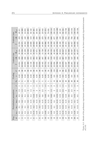
Shortages of law enforcement infrastructure, large jurisdiction coverage areas, high operating
costs of MLE resources, the requirement of using complex threat detection and evaluation sys-
tems, scarce maritime intelligence and a lack of adequately trained operators are examples of
factors contributing to the difficulty of effective MLE by coastal nations, inevitably affecting
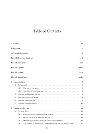
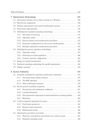
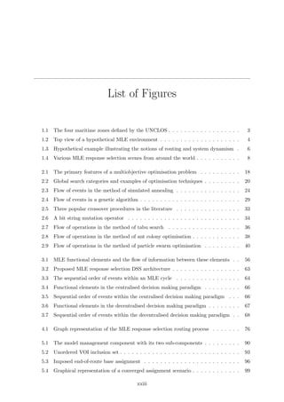
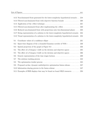
their overall ability to achieve effective counter-threat performance at sea. A simplified hypo-
thetical MLE scenario, depicting the kind of visual information that an MLE response selection
operator may be observing on a human-computer interface in order to assist him in making
MLE response selection decisions, is portrayed in Figure 1.2.
Active MLE Resources
Idle MLE Resources
VOIs
Bases
Patrol Circuits
MLE Boundaries
LandSea
Figure 1.2: Top view of a hypothetical MLE environment.
MLE operations often comprise complex tasks, typically involving a number of explicitly or
implicitly identified subtasks, each with specific resource capability requirements that need to
be matched with the capabilities of available MLE resources in order to ensure successful VOI
interception [54]. These tasks are stochastically distributed in both time and space, making the](https://image.slidesharecdn.com/6cd1ebf5-5cfe-4d40-998c-99cbe17b08f1-170109122537/85/PhD-dissertation-36-320.jpg)
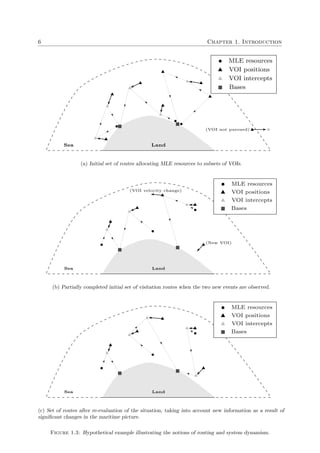
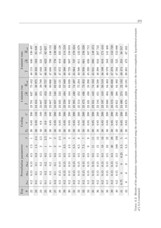
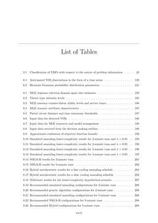
![8 Chapter 1. Introduction
(a) Light, high-speed patrol vessel used in waters
around Cape Town [22].
(b) Various types of MLE resources available to
the Canadian Coast Guard [57].
(c) US coast guards in the process of setting up
several MLE resources prior to dispatch [94].
(d) Seaplanes are effective scouts when deployed
in parallel with long-range MLE resources [94].
(e) Unmanned airplanes are popular for acquiring
threat evaluation information [70].
(f) Interception of a suspicious boat thought to
carry ammunition off the coast of Somalia [59].
(g) Preventative measures against a potential oil
spill situation off the Panama coast [99].
(h) Combined assignment of MLE resources onto
a high-alert VOI in the East-China sea [63].
Figure 1.4: Various MLE response selection scenes from around the world.](https://image.slidesharecdn.com/6cd1ebf5-5cfe-4d40-998c-99cbe17b08f1-170109122537/85/PhD-dissertation-40-320.jpg)
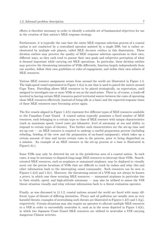
![1.3. Dissertation aim and scope 9
1.3 Dissertation aim and scope
The aim in this dissertation is to contribute on an advanced research level to coastal MLE re-
sponse selection and routing decision infrastructure in the form of the design of a semi-automated
DSS capable of assisting human operators in spatio-temporal resource dispatch decision making
so that MLE resources may be employed effectively and efficiently. As explained in §1.2, these
decisions are made based on input data (which are assumed throughout this dissertation to
be complete and accurate) obtained from the threat detection and threat evaluation systems
employed with a view to analyse the potentially threatening behaviour of vessels observed at
sea at any given time, as well as subjective input data contributed by MLE response selection
operators2. Automated decision making is therefore not pursued as the aim of this study is to
provide a support tool to a human operator.
The multiple objectives component of the proposed DSS will be incorporated in the system in a
generic manner, so as to provide users of the system with the freedom of configuring their own,
preferred goals. This generic DSS design will be populated with examples of models capable of
performing the functions of the various constituent parts of the system, and their workability
will be tested and demonstrated by solving the MLE response selection problem in the context
of realistic, but simulated, practical scenarios, employing multiple solution search techniques.
These examples may, of course, be replaced with more desirable or better performing features,
were such a DSS to be implemented in a realistic environment in the future.
Although difficult to measure against a simple MLE response selection human operator in terms
of performance, this system may be used in the future to assist such an operator in his decision
making process. In particular, the operator may use it as a guideline to validate and/or justify
his decisions when the level of uncertainty pertaining to the observed maritime scenario is high
and/or if only parts of the problem may be solved with the sole use of his competence and
expertise in the field. Overall, usage of this system in a real-world context may reduce operator
stress levels typically associated with difficult decisions, while improving the overall performance
of MLE operations in an integrated fashion across multiple decision entities.
The research hypothesis of this dissertation is therefore as follows: Semi-automated decision
support based on mathematical modelling principles may be used to assist in making better deci-
sions in an MLE response selection context than those based purely on subjective human operator
judgment.
1.4 Dissertation objectives
The following objectives are pursued in this dissertation:
I To compile a literature survey of the theoretical concepts underlying the design of an MLE
response selection and routing DSS, by
(a) discussing the nature of decision making procedures in general,
(b) presenting an array of popular stochastic search techniques used to solve complex
discrete optimisation problems,
(c) elaborating on the workings of two such techniques in the context of multiobjective
optimisation,
2
This process is better known as a “human in the loop” approach to decision making [49].](https://image.slidesharecdn.com/6cd1ebf5-5cfe-4d40-998c-99cbe17b08f1-170109122537/85/PhD-dissertation-41-320.jpg)

![CHAPTER 2
Literature Review
Contents
2.1 Decision theory . . . . . . . . . . . . . . . . . . . . . . . . . . . . . . . . . . . . 13
2.2 Optimisation techniques . . . . . . . . . . . . . . . . . . . . . . . . . . . . . . . 19
2.3 The method of simulated annealing . . . . . . . . . . . . . . . . . . . . . . . . . 22
2.4 Evolutionary algorithms . . . . . . . . . . . . . . . . . . . . . . . . . . . . . . . 27
2.5 Other popular metaheuristics . . . . . . . . . . . . . . . . . . . . . . . . . . . . 34
2.6 The vehicle routing problem . . . . . . . . . . . . . . . . . . . . . . . . . . . . . 39
2.7 Dynamic multiobjective optimisation approaches . . . . . . . . . . . . . . . . . 46
2.8 MLE DSSs in existence . . . . . . . . . . . . . . . . . . . . . . . . . . . . . . . 49
2.9 Chapter Summary . . . . . . . . . . . . . . . . . . . . . . . . . . . . . . . . . . 53
This chapter contains a review of the literature on topics related to the design of a DSS for as-
sisting operators in their complex MLE response selection decisions. The purpose of the chapter
is to provide the reader with the necessary background in order to facilitate an understanding
of the material presented in the remainder of this dissertation.
In §2.1, a discussion is conducted on the philosophy and fundamental concepts behind decision
making, while an overview of solution techniques for optimisation problems is provided in §2.2,
with particular emphasis on the use of metaheuristics. The methods of simulated annealing and
evolutionary algorithms are then presented in more detail in §2.3 and §2.4, respectively, and this
is followed by a general description of three other innovative metaheuristic search techniques in
§2.5. A review of routing problems with emphasis on dynamic and stochastic routing problems
may be found in §2.6. In §2.7, a closer look is taken at various approaches used in the literature
toward solving multiobjective dynamic optimisation problems, while the focus turns in §2.8 to
a review of MLE semi or fully automated DSSs in existence. The chapter finally closes with a
brief summary in §2.9.
2.1 Decision theory
The etymology of the term decision derives from the Latin word decidere, which means to decide
or to determine. This word consists of the words de, which means “off”, and caedere, which
means “to cut” [30]. According to this description, decision making is the process whereby
plausible alternatives with respect to the course of actions to be taken when exposed to a
13](https://image.slidesharecdn.com/6cd1ebf5-5cfe-4d40-998c-99cbe17b08f1-170109122537/85/PhD-dissertation-45-320.jpg)
![14 Chapter 2. Literature Review
certain situation are rejected from a finite set of choices (i.e. cut-off) until all that remains is
a most desirable alternative to be executed as a response to the situation. This definition is
particularly applicable in the field of operations research, in which the feasible decision space of
a problem is traditionally analysed, or “searched”, and alternative solutions to the problem are
rejected according to a certain sequence of rules until a single (i.e. most preferred) alternative
(or set of alternatives) remains. Decision making is a critical component in almost any situation.
Although most decisions take place on the subconscious level, the ability to make high-quality
choices under uncertainty may usually only be realisable with the use of some complex analytical
process.
2.1.1 Elementary concepts of decision making
In decision making, a goal may be thought of as a purpose towards which an endeavor is directed,
while an objective may be thought of as a specific result or results that a person or system aims
to achieve within a certain time frame and with available resources. Whereas goals do not
necessarily have to be measurable or tangible, objectives are expected to be so [46]. The choice
of alternatives in a decision making situation should be measurable in terms of evaluative criteria.
A criterion is a principle or standard which provides a means to compare a set of alternatives
on the basis of some particular aspect that is relevant or meaningful to the decision maker(s)
[27]; they help define, on the most fundamental level, what “best” really means. Objectives are
measured on suitable attribute scales, which provide a means to evaluate the quality of each
alternative with respect to every criterion relevant to the decision problem.
In order to identify these criteria, it is critical to first determine and assess the basic values of
the decision maker with respect to the situation at hand (i.e. what really matters to him) [27].
Values underlie decision making in a fundamental manner; if a decision maker does not care
about the criteria, there would be no reason for him to make a decision in the first place, as he
would be completely indifferent with respect to assessing the desirability of alternative solutions.
Objectives are therefore necessary in order to establish a direct relationship with one or more
particular criteria in terms that relate directly to the basic values of the decision maker. In the
field of operations research, analysts and consultants unfortunately often neglect such values,
instead tending to solve a decision making problem with respect to what they think is deemed
important, and thereby disregarding certain critical aspects associated with the psychological
needs and preferences of their clients1 [61].
In general, the goal in any decision making process is to seek the best alternative by considering
all decision-impacting criteria simultaneously whilst acknowledging decision space delimitations.
Incorporating these criteria, as well as the values of the decision maker, in the process is achieved
by configuring the objective(s) accordingly. As hinted at previously, every decision making
situation is relevant within a specific context, which calls for specific objectives to be considered.
A criterion may either be advantageous or disadvantageous with respect to the preferences
of the decision makers; alternatives simultaneously minimising or maximising each criterion,
respectively, are therefore sought.
2.1.2 On the decision structuring process
According to Clemen & Reilly [27], modelling a decision making problem consists of three
fundamental steps: (1) identifying the values of the decision maker with respect to the problem
1
This discrepancy has given rise to the field of behavioural operational research over the last decade.](https://image.slidesharecdn.com/6cd1ebf5-5cfe-4d40-998c-99cbe17b08f1-170109122537/85/PhD-dissertation-46-320.jpg)
![2.1. Decision theory 15
at hand and defining all objectives so as to correctly integrate the decision model, (2) structuring
the elements of the decision making problem into a logical framework, and (3) defining and fully
refining all the elements of the model.
Furthermore, the set of objectives should include all relevant aspects of the underlying decision
yet be as small as possible (so as to avoid unnecessary computational complexity). The set
of objectives should therefore not contain redundant elements and should be decomposable2.
Finally, the objectives should be clearly distinguishable and the relevant attribute scales should
provide a simple way of measuring the performance of alternatives with respect to the objectives.
Generally speaking, objectives may either be categorised as fundamental or mean [27]. Fun-
damental objectives are the basis on which various alternatives may be measured (the type
of objectives discussed in the previous section). Mean objectives, on the other hand, are of a
purely intermediate nature, and are used to help achieve other objectives. While fundamental
objectives are organised into hierarchies, which are crucial for the development of a multiobjec-
tive decision model, mean objectives are usually organised in the form of networks (similar to a
brainstorming configuration).
Influence diagrams and decision trees are examples of techniques often used to structure the
decision making process into a logical framework [27]. An influence diagram captures the decision
maker’s current state of knowledge by providing a simple graphical representation of the decision
situation. In such a diagram, the decision process is represented as various shapes, interlinked
by directed arcs in specific ways so as to reflect the relationship among the decision components
in a relevant, sequential order. Although appropriate for displaying a decision’s basic structure,
influence diagrams tend to hide details. A decision tree, on the other hand, expands in size
and level of detail in a time sequence as the decision process evolves. Such a tree represents all
possible paths that the decision maker might follow throughout the decision making process,
depicting all alternative choices, as well as consequences resulting from uncertain events. The
alternatives, represented by branches leaving a decision node, must be such that only one option
can be chosen, while the branches leaving uncertain event nodes must correspond to a set of
mutually exclusive and collectively exhaustive outcomes (that is, at most one outcome may
occur from a finite set of outcomes with specific probabilities, and at least one of these outcomes
has to occur). Overall, both influence diagrams and decision trees have their own advantages
for structuring the decision making process. Their combined use in parallel during the decision
making process, however, provides a complete model of the decision framework. One may
therefore think of them as complementary rather than competitors in structuring a decision
making process.
2.1.3 Decision making with multiple conflicting objectives
Multiobjective decision making problems occur in most disciplines. Despite the considerable va-
riety of techniques that have been developed in the field of operations research since the 1950s,
solving such problems has presented a non-trivial challenge to researchers. Indeed, the earli-
est theoretical work on multiobjective problems dates back to 1895, when the mathematicians
Cantor and Hausdorff laid the foundations of infinitely dimensional ordered spaces [72]. Cantor
also introduced equivalence classes and utility functions a few years later [29], while Hausdorff
published the first example of a complete ordering set [29].
In most decision making situations, the decision maker is required to consider more than one
2
A set of objectives is decomposable if the decision maker is able to think about each objective easily without
having to consider the others simultaneously.](https://image.slidesharecdn.com/6cd1ebf5-5cfe-4d40-998c-99cbe17b08f1-170109122537/85/PhD-dissertation-47-320.jpg)
![16 Chapter 2. Literature Review
criterion simultaneously in order to build a complete, accurate decision making model. These
criteria, however, typically conflict with one another as informed by the values of the decision
maker. Objectives are said to be conflicting if trading an alternative with a higher achievement
measure in terms of a certain criterion comes at a cost (i.e. a decrease in the levels of achievement
of some of the other criteria for that alternative). A crucial problem in multiobjective decision
making therefore lies in analysing how to best perform trade-offs between the values projected
by these conflicting objectives.
There exist multiple techniques for determining the quality of an alternative in a decision making
process [27]. An appropriate technique should be selected based on factors such as the complexity
of the problem, the nature of the decision maker, the time frame for solving the problem or the
minimum quality level of the best alternative. The additive preference model, for example, is a
popular method in the literature [43, 117], in which the decision maker is required to construct
a so-called additive utility function for comparing the attribute levels of available alternatives,
as well as the fundamental objectives, in terms of their relative importance, using weight ratios.
This decision making model approach is, however, incomplete, as it ignores certain fundamental
characteristics of choice theory amongst multiatribute alternatives [27]. In order to resolve this
discrepancy, slightly more complex methods such as multiattribute utility models were designed
[104]. Here, the decision maker considers attribute interactions by establishing sub-functions
for all pairwise combinations of individual utility functions, in contrast to utilising an additive
combination of preferences for individual attributes.
In general, the approach adopted toward solving a multiobjective decision making problem may
be classified into two paradigms [27, 81]. The first involves combining the individual objective
functions into a single composite function, or to move all except one objective to the set of
constraints. This is typically the case in utility theory and weighted sum methods. The additive
utility function and multiattribute utility models mentioned above, are examples of decision
making techniques in this paradigm. Optimisation methods in this paradigm therefore return
a single “optimal” solution to a multiobjective decision making problem. This procedure of
handling multiobjective optimisation problems is a relatively simple one. Due to the subjective
nature of the decision making problem in terms that depend purely on the decision maker’s pref-
erences, however, it may often be very difficult to determine all the necessary utility functions
and weight ratio parameters accurately, particularly when the number of attributes to be consid-
ered is large. Perhaps more importantly, parts of the front are inaccessible when adopting fixed
weights in the case of non-convex problems [42]. This optimisation procedure may be enhanced
to some extent by considering multiple a priori weight vectors; this is particularly useful in
cases where choosing a single appropriate set of weight ratio parameters is not obvious. In most
non-linear multiobjective problems, however, it has been shown that a uniformly distributed set
of weight vectors need not necessarily result in a uniformly distributed set of Pareto-optimal
solutions [42]. Once again, since the nature of this mapping is not usually known, it is often
difficult to select weight vectors which are expected to result in a Pareto-optimal solution located
within some desired region of the objective space.
Alternatively, the second paradigm, referred to as multiobjective optimisation, aims to enumer-
ate and filter the set of all alternatives into a suggested decision set in such a way that the
decision maker is indifferent between any two alternatives within the set and so that there exists
no alternative outside the set which is preferred to any alternatives within the set. Due to the
conflicting nature of the objectives, no single solution typically exists that minimises or max-
imises all objectives simultaneously. In other words, each alternative in the suggested decision
set yields objective achievement measures at an acceptable level without being outperformed by
any other alternatives [81]. Decision making techniques within this paradigm therefore aim to](https://image.slidesharecdn.com/6cd1ebf5-5cfe-4d40-998c-99cbe17b08f1-170109122537/85/PhD-dissertation-48-320.jpg)
![2.1. Decision theory 17
identify a set of alternative solutions which represent acceptable inter-attribute compromises.
This approach is elucidated in the following section. One of the principal advantages of multiob-
jective optimisation is that the relative importance of the objectives can be decided a posteriori
with the Pareto front on hand.
2.1.4 The notions of dominance, Pareto optimality and the Pareto front
In contrast to single objective optimisation problems, in which a single, optimal solution is
sought, multiobjective problems induce a set of alternative solutions in the decision space of
the problem which, when evaluated, produce vectors whose components represent trade-offs in
the multidimensional objective space of the problem. As described in the previous section, the
objectives being optimised in a multiobjective optimisation problem usually always conflict with
one another, placing a partial, rather than total, ordering on the search space [29].
Consider a multiobjective optimisation model consisting of n decision variables x1, . . . , xn with
respective restricting lower and upper bound values (x
(L)
1 , x
(U)
1 ), . . . , (x
(L)
n , x
(U)
n ), m constraints
with standardised evaluative functions g1, . . . , gm, k objectives with evaluative functions f1, . . . , fk
mapping the n-dimensional vector x = (x1, . . . , xn) in decision space (or solution space) to the
k-dimensional vector f(x) = (f1(x), . . . , fk(x)) in objective space. This mapping may or may
not be surjective, depending on the evaluative functions and constraint configurations [42]. The
multiobjective optimisation problem in its general form may be stated as:
Minimise/Maximise fo(x), o ∈ 1, 2, . . . , k,
subject to gc(x) ≤ 0, c ∈ 1, 2, . . . , m,
x
(L)
i ≤ xi ≤ x
(U)
i , i ∈ 1, 2, . . . , n.
Let Ψ ⊆ n be a compact set representing the feasible decision space of the maximisation
problem described above, and let Φi ⊆ represent the feasible objective space with respect to
the ith objective function; i.e. fi : Ψ → Φi. Then, x∗ ∈ Ψ is a global maximum with respect to
fi if and only if fi(x∗) ≥ fi(x) for all x ∈ Ψ.
The notion of a global optimum for the ith objective function may be extended to the full
multiobjective optimisation problem in the following way. A decision vector x ∈ Ψ is said to
dominate a decision vector y ∈ Ψ, denoted here by x y, if fi(x) ≥ fi(y) for all i ∈ {1, . . . , k}
and if there exists at least one i∗ ∈ {1, . . . , k} such that fi∗ (x) > fi∗ (y). It follows that any two
candidate solutions to the mulitobjective problem described above are related to each other in
two possible ways only: (1) either one dominates the other, or (2) neither one is dominated by
the other. Moreover, x is said to be non-dominated with respect to the set Ψ ⊆ Ψ if there exist
no vectors y ∈ Ψ such that y x. Finally, a candidate solution x is said to be Pareto optimal
if it is non-dominated with respect to the entire decision space Ψ.
According to the above definition, Pareto optimal solution vectors therefore represent trade-off
solutions which, when evaluated, produce vectors whose performance measure in one dimension
cannot be improved without detrimentally affecting at least some subset of the other k − 1
dimensions. The Pareto optimal set P is, henceforth, defined as the set of candidate solutions
containing all Pareto optimal solutions in Ψ. That is,
P = {x ∈ Ψ | y ∈ Ψ such that y x}.
Pareto optimal solutions may have no obvious apparent relationship besides their membership
of the Pareto optimal set; such solutions are purely classified as such on the basis of their values](https://image.slidesharecdn.com/6cd1ebf5-5cfe-4d40-998c-99cbe17b08f1-170109122537/85/PhD-dissertation-49-320.jpg)
![18 Chapter 2. Literature Review
in objective space. These values produce a set of objective function vectors, known as the Pareto
front F, whose corresponding decision vectors are elements of P. That is,
F = {f(x) | x ∈ P}.
A graphical illustration of certain concepts discussed above is provided in Figure 2.1 for a
multiobjective problem for which n = 3, k = 2 and m = 6. Here, elements from the cubic
feasible solution space Ψ ⊂ 3 (delimited by the dashed planes), are mapped to the pentagonal
objective space Φ ⊂ 2. The Pareto front is denoted by the bold curve in objective space.
Moreover, all objectives are here assumed to be computable functions available in closed form
which have to be maximised.
x1
x3
x2
x
Ψ
(a) Solution space (b) Objective space
f1
f2 f(x)
Φ
f
Figure 2.1: Graphical example of the primary features of a multiobjective problem with n = 3 deci-
sion variables constrained by m = 6 constraints, k = 2 and objective functions f1, f2 which are to be
maximised. The Pareto front is denoted by the bold curve in objective space.
2.1.5 Multiperson decision making
In most decision making situations, the outcome of the decision directly or indirectly affects
more than just the decision maker; although he might be the only one responsible for ultimately
making the decision, regardless of the impact of the decision outcome on other individuals. In
certain cases, however, the decision maker may wish to analyse how the outcome of a particu-
lar decision affects a group of individuals, or he may consider individual preferences as part of
the decision making process. Alternatively, several decision makers may carry out the decision
making process together, with the aim of reaching some form of consensus or agreement. De-
cisions involving the contribution of multiple members or parties in a decision making process
are defined in the literature as multiperson decision making problems [65].
Examples of two well-known techniques (from opposite ends of the methodological spectrum) for
solving multiperson decision making problems are majority voting and consensus attainment.
Whereas in majority voting, agreement by a set majority of members is sufficient to reach a
final decision, most or all members must reach a certain level of mutual agreement in order for
the decision process to move forward in a consensus attainment process.
Consensus attainment therefore deals with the cooperative process of obtaining the maximum
degree of agreement between a number of decision makers with respect to selecting and sup-](https://image.slidesharecdn.com/6cd1ebf5-5cfe-4d40-998c-99cbe17b08f1-170109122537/85/PhD-dissertation-50-320.jpg)
![2.2. Optimisation techniques 19
porting a solution from a given set of alternatives, for the greater good of the situation at hand.
In practice, the consensus process is typically a dynamic and iterative group discussion process,
usually coordinated by a moderator, responsible for helping the members to bring their opinions
closer to one another [65]. During each step of the process, the moderator keeps track of the ac-
tual level of consensus between the decision makers, typically by means of some pre-determined
consensus measure establishing the distance from the current consensus level to the ideal state
of consensus (i.e. full and unanimous agreement of all members with respect to a specific alter-
native). If the current consensus level is deemed unacceptable, that is, if it is lower than some
pre-determined threshold level, indicating that there exists a considerable degree of discrepancy
between the decision makers’ opinions, then the moderator asks the members to discuss their
opinions further in an effort to bring them closer to consensus. The consensus attainment deci-
sion making process is also sometimes able to function without the use of a moderator, whose
inclusion in the process may be too time-consuming, but is rather controlled automatically by
the group, receiving input from the various decision makers, assessing the consensus level at
each step of the process, and providing feedback (output) on the current state and progress of
the process back to the decision makers.
According to Bressen [14], while majority voting typically leads to a (technically) much simpler
and faster decision making process than does consensus attainment, consensus attainment offers
three major advantages over majority voting. First, consensus attainment leads to more effective
implementation (when all decision makers’ ideas and concerns are accounted for, they are more
likely to participate actively towards making something happen). In majority voting, on the
other hand, members with a minority position are usually overruled and are naturally unwilling
to participate in the decision process with much eagerness. Secondly, consensus attainment
builds connections amongst decision makers (using consensus attainment suggests that some
time is taken to achieve a certain level of agreement amongst the members on how to proceed
with the decision making process before actually moving forward). Majority voting, on the other
hand, creates winners and losers, which has a dividing effect amongst the decision makers [14].
Lastly, consensus attainment usually leads to higher quality decisions (integrating the wisdom
and experience of all members into the decision making process typically generates better and
smarter decisions than majority voting does, particularly when the decision makers are assumed
to be rational).
2.2 Optimisation techniques
In this section, an overview is provided of general search techniques aimed at finding exact or
approximate solutions to optimisation problems. This is followed by a more elaborate discussion
on the class of stochastic search techniques, members of which are later implemented in this
dissertation. There does, however, not seem to be full consensus on a standard classification for
optimisation search methods in the literature.
According to Coello et al. [29], one way to differentiating between different types of solution
search and optimisation techniques is to classify them as enumerative, deterministic or stochastic.
Such techniques may further be classified as exact, heuristic or metaheuristic [153]. Examples of
popular search techniques in these categories are listed in Figure 2.2. Other classifications of op-
timisation techniques may also include partitions according to traditional versus non-traditional,
local versus global or sequential versus parallel techniques.
Full enumeration techniques evaluate every possible solution in the solution space of the op-
timisation problem, either explicitly or implicitly. If the problem complexity is relatively low](https://image.slidesharecdn.com/6cd1ebf5-5cfe-4d40-998c-99cbe17b08f1-170109122537/85/PhD-dissertation-51-320.jpg)
![20 Chapter 2. Literature Review
StochasticDeterministicEnumerative
Exact
Heuristic
Metaheuristic
Full Depth First Search
Full Breadth First Search
Full Branch-and-Bound
The Simplex Algorithm Full Simulated Annealing
Rule-Based
Partial Enumeration
Greedy Heuristics
Gradient Methods
Random Walk
Monte Carlo Simulation
Intelligent
Partial Enumeration
Tabu Search
Truncated Simulated Annealing
Particle Swarm Optimisation
Ant Colony Optimisation
Evolutionary Algorithms
Figure 2.2: Global search categories and examples of techniques.
and the search can be performed within a reasonable amount of time, then these techniques are
guaranteed to find a global optimum. Adopting this kind of approach when solving an optimisa-
tion problem is typically extremely straightforward and easy to apply. Enumeration approaches
may, however, be entirely insufficient when dealing with large optimisation problems.
Deterministic search techniques overcome the problem of a large search space, by incorporating
the notion of problem domain knowledge to reduce the size of the search space. Here, the aim is to
implement some means of guiding or restricting the search space in order to find good solutions
within an acceptable time. Although proven to be successful methods for solving a wide variety
of problems, the complex features associated with many real-world optimisation problems, such
as multimodality3, highly dimensionality, discontinuous and/or NP-completeness, often cause
deterministic methods to be ineffective for solving problems of this kind4 over large search
spaces, due to their dependence on problem domain knowledge for guiding the search process
[29].
Stochastic search techniques were developed as an alternative for solving such irregular problems.
Here, the subsequent state of the search process is induced probabilistically (i.e. randomly)
instead of deterministically. These techniques are based on probabilistic sampling of a set of
possible solutions and, throughout the search, maintain some form of record of good solutions
found. A predetermined function assigning performance values to candidate/partial solutions as
well as a mapping mechanism linking the problem domain to the algorithm is required. Given
3
A problem is said to be multimodal if it contains an objective function with more than one optimum (i.e. one
or more global optimum in addition to one or more local optimum of inferior quality) [162].
4
Problems exhibiting one or more of these characteristics are sometimes called irregular [29].](https://image.slidesharecdn.com/6cd1ebf5-5cfe-4d40-998c-99cbe17b08f1-170109122537/85/PhD-dissertation-52-320.jpg)
![2.2. Optimisation techniques 21
the level of complexity of some irregular multiobjective problems, stochastic methods are often
able to yield satisfactory solutions to such problems for which the search space is not chaotic5.
Metaheuristics have recently become very popular for solving multiobjective optimisation prob-
lems. A metaheuristic is a state-of-the-art search technique which may be defined as a higher-
level procedure designed to strategically guide one or more lower-level procedures or heuristics to
search for feasible solutions in spaces where the search task is hard [31]. Metaheuristics are char-
acterised by their typically approximate, stochastic and non problem-specific nature. According
to Suman and Kumar [138], the increasing acceptance of these search techniques is a result of
their ability to: (1) find multiple candidate solutions in a single run, (2) function without the
use of derivatives, (3) converge with great speed and accuracy towards Pareto optimal solutions,
(4) accommodate both continuous and combinatorial optimisation problems with relative ease
and (5) be less affected by the shape or continuity of the Pareto front.
One way of classifying metaheuristics is to refer to their search strategies, which, according to
Blum and Roli [7], is either trajectory-based or population-based. These categories are typically
characterised by the number of candidate solutions generated during every iteration of the search
process. Trajectory-based metaheuristics start with a single initial candidate solution and, at
every iteration, replace the current solution by a different, single candidate solution in its neigh-
bourhood (examples of such metaheuristics include simulated annealing [138], tabu search [48]
and variable neighbourhood search [123]). Population-based metaheuristics, on the other hand,
start with an initial population of multiple candidate solutions, which are enhanced through
an iterative process by replacing part of the population with carefully selected new solutions
(examples of such metaheuristics include genetic algorithms [29], ant colony optimisation [47]
and particle swarm optimisation [114]). Trajectory-based approaches are usually able to find
locally optimal solutions quickly, and are thus often referred to as exploitation-oriented meth-
ods. Population-based approaches, on the other hand, strongly promote diversification within
the search space, and are thus often referred to as exploration-oriented methods. Additionally,
population-based approaches often incorporate a learning component.
Other classes of stochastic search techniques include hybrid metaheuristics, parallel metaheuris-
tics and hyperheuristics. A hybrid metaheuristic typically combines several optimisation ap-
proaches (such as other metaheuristics, artificial intelligence, or mathematical programming
techniques) with a standard metaheuristic. These approaches run concurrently with one an-
other, and exchange information, in order to guide the search process. Parallel metaheuristics,
on the other hand, use the techniques of parallel programming to implement multiple meta-
heuristic searches in parallel so as to guide the search process more effectively. Hyperheuristics
were initially introduced to devise new algorithms for solving problems by combining known
search techniques in ways that allow each of them to compensate, to some extent, for the weak-
nesses of others [17]. Their goal is to be generally applicable to a large range of problems by
performing well in terms of computational speed, solution quality, repeatability and favourable
worst-case behaviours, in cases where standard metaheuristic techniques fail to perform well on
some of these counts.
In the following three sections, five metaheuristics are presented in varying amounts of detail.
For reasons that will later become apparent, simulated annealing and evolutionary algorithm
techniques are discussed in more detail and are reviewed in the context of both single- and
multiobjective optimisation problems, while the remaining algorithms are only briefly discussed
in the context of single-objective optimisation problems.
5
A problem is said to be chaotic if small differences in initial conditions yield widely diverging outcomes in
the long run, rendering long-term predictions near-impossible [149].](https://image.slidesharecdn.com/6cd1ebf5-5cfe-4d40-998c-99cbe17b08f1-170109122537/85/PhD-dissertation-53-320.jpg)
![22 Chapter 2. Literature Review
2.3 The method of simulated annealing
The method of simulated annealing is a metaheuristic that exploits the deep and useful con-
nection between statistical mechanics and large combinatorial optimisation problems. It was
initially developed for use in the context of highly non-linear optimisation problems [18, 78].
Statistical mechanics may be described as the central discipline of condensed matter physics,
embodying methods for analysing aggregate properties of the large number of molecules to be
found in samples of liquid or solid matter.
The notion of simulating the evolution of the state of a system towards its thermodynamic
equilibrium at a certain temperature dates back to the work of Metropolis et al. [100] in 1953.
In their paper, they present an algorithm (now called the Metropolis algorithm) which simulates
the behaviour of a collection of molecules in thermodynamic equilibrium at a given temperature.
Each iteration of this process consists of moving an atom by a small random displacement,
consequently generating a certain change ∆E in the energy state of the system. If the move
results in a decrease in the energy of the system, it is accepted. If the move results in an increase
in the energy of the system, it is accepted with a probability exp(−∆E
T ), where T represents the
current temperature of the system. This occasional increase in objective function value prevents
the system from becoming trapped at a local optimum. Repeating this process generates a
sequence of configurations which may be modelled as a Markov chain, in which a certain state
of the chain represents a state of energy corresponding to its respective system configuration,
eventually causing the system to reach a thermodynamic equilibrium6. Once a thermodynamic
equilibrium at a particular temperature is reached, the temperature is lowered according to a
cooling schedule and a new Markov chain of energy states is configured for that new temperature.
2.3.1 The notion of annealing
A fundamental question in statistical mechanics, evolves around the behaviour of a system as
the temperature decreases (for example, whether the molecules remain fluid or solidify). From
a practical point of view, low temperature is not a sufficient condition for seeking ground states
of matter such as crystalline solids [78]. Experiments that determine such states are conducted
according to the process of annealing.
Annealing involves the heating and cooling of a material to alter its physical properties as a
result of the changes in its internal structure [71]. It is initiated by heating a material to a
certain temperature in order to convey a certain level of thermal energy to it. The material is
then cooled in stages according to a specific schedule. During this process, the temperature of
the material is carefully controlled so that the material spends a significant amount of time close
to its freezing point. In doing so, the particles of a solid first randomly rearrange themselves
once a liquid stage is reached during the melting phase, and then form a crystalised solid state as
the temperature is slowly lowered during the cooling phase. The annealing process is terminated
when the system reaches a solidified state.
At high temperatures, a material in liquid form allows the molecules to rearrange themselves
with more freedom, hence increasing the potential combination of inter-molecular moves. Low
temperatures, on the other hand, cause the molecules to become more confined due to high
energy costs of movement, therefore only allowing a limited amount of possible moves to be
conducted in the system. Every time a molecule is moved while a system is in equilibrium,
6
This research later on allowed for the population of the so-called Boltzman distribution of the energy states
at a specific temperature to be extracted [48].](https://image.slidesharecdn.com/6cd1ebf5-5cfe-4d40-998c-99cbe17b08f1-170109122537/85/PhD-dissertation-54-320.jpg)
![2.3. The method of simulated annealing 23
a certain amount of energy is released, causing the energy level of the system to change in
accordance with the motion of that molecule. A sudden change in the energy state of a system
is known as a perturbation.
In solidified form, the material is uniformly dense and contains almost no structural flaws. In
order for the crystal lattices to form in a suitably organised manner, however, the energy level
released in the system during the cooling process has to be as small as possible as it approaches
this state. Quickly lowering the temperature, known as quenching, causes the material to be
out of equilibrium as it reaches the state, resulting in low crystalline order or locally optimal
structure which ultimately causes defects in the formation of the crystals [78].
2.3.2 Algorithm outline
The annealing process discussed in the previous section exhibits analogies with the solution
of combinatorial optimisation problems. Here, a control parameter mimicking the role of the
temperature is introduced in the optimisation process. This parameter must have the same
effect as the temperature of the physical system in statistical mechanics, namely conditioning the
accessibility of energy states (i.e. objective function achievement measures), and lead towards a
globally optimal state of the system (i.e. a globally optimal solution), provided that it is lowered
in a carefully controlled manner. The final solution obtained is analogous to a solidified form of
the system.
Under the Metropolis acceptance rule, the role of the temperature in simulated annealing is now
more clear. Assuming a minimisation problem, exp(−∆E
T ) → 1 as T → ∞, suggesting that many
solutions are accepted while the temperature is high7. The algorithm therefore performs similarly
to a simple random walk search during these early stages, which greatly favours exploration of
the search space. On the other hand, the probability of accepting non-improving moves decreases
as the temperature decreases, suggesting that solutions degrading the objective function are less
likely to be accepted as the next configuration state in the system, but nevertheless giving
the system a small chance to be perturbed out of a local optimum. Non-improving moves are
accepted according to a so-called probability acceptance function, which may or may not be the
Metropolis acceptance rule.
Lowering the temperature is controlled according to a so-called cooling schedule. Careful con-
sideration must be given to the nature of the cooling schedule; lowering the temperature too
quickly lowers the chances of accepting solutions too quickly which may cause large parts of the
solution space to remain unexplored, while lowering the temperature too slowly may result in the
consideration of many redundant solutions which do not lead to a high-quality non-dominated
front in objective space.
Therefore, as the temperature is reduced, only perturbations leading to small decreases in energy
are accepted, so that the search is limited to a smaller subset of the solution space (i.e so that
exploitation of good regions of the solution space occurs) as the system hopefully settles on a
global minimum. The analogy of simulated annealing therefore evolves around the assumption
that if the move probability decreases slowly enough, a global optimum may be found. If
quenching occurs, however, the search is more likely to lead to a local minimum.
A flowchart of the process of simulated annealing is presented in Figure 2.3. Here, the outer
loop controls the temperature schedule, while the inner loop attempts to reach a thermodynamic
equilibrium according to the Metropolis algorithm. In addition, a pseudo-code description of the
basic working of the method of simulated annealing is given in Algorithm 2.1. In the outlined
7
In a maximisation problem, moves are accepted with probability 1 if they increase the energy of the system.](https://image.slidesharecdn.com/6cd1ebf5-5cfe-4d40-998c-99cbe17b08f1-170109122537/85/PhD-dissertation-55-320.jpg)
![24 Chapter 2. Literature Review
simulated annealing algorithm, a move refers to a modification made to the current solution. The
algorithm keeps track of the best solution found thus far during the search, called the incumbent
solution. Once the system reaches a solidified state, the incumbent solution is reported as an
approximate solution to the optimisation problem.
Generate initial solution
Set initial temperature
Perturb current solution
∆E ≤ 0 ? Accept move
TrueAccept move with
probability e
−∆E
T
False
Thermodynamic
equilibrium?
False
True
System
solidified?
Lower temperature
according to
cooling schedule
False Report
incumbent solution
True
Figure 2.3: Flow of events in the simulated annealing algorithm for a minimisation problem.
2.3.3 Multiobjective simulated annealing
It is possible to compare the relative quality of two vector solutions with the dominance
relation, but note that it gives, essentially only three values of quality — better, worse,
equal — in contrast to the energy difference in uni-objective problems which usually
give a continuum. — K. Smith [130]
The method of simmulated annealing may also be used to solve multiobjective problems in which
the decision maker is eventually presented with an acceptable set of non-dominated solutions.](https://image.slidesharecdn.com/6cd1ebf5-5cfe-4d40-998c-99cbe17b08f1-170109122537/85/PhD-dissertation-56-320.jpg)
![2.3. The method of simulated annealing 25
Algorithm 2.1: Simulated annealing algorithm outline (for a minimisation problem)
Generate initial feasible solution1
while System not solidified (i.e. T > 0) do2
while Thermodynamic equilibrium not reached do3
Generate neighbouring solution (i.e. perturb current solution)4
Evaluate the change in energy ∆E resulting from the perturbation5
if ∆E ≤ 0 then6
Accept the move and make the neighbouring solution the current solution7
else8
Accept the move with probability e
−∆E
T9
Lower temperature according to the cooling schedule10
Report incumbent solution11
Just like in single-objective optimisation problems, most multiobjective simulated annealing
algorithms have the advantage that they allow for a broad search of the solution space at first,
before gradually restricting the search so as to decrease the acceptance of non-improving moves
later on during the search.
In multiobjective problems, generating neighbouring moves via simulated annealing can result
in one of three different outcomes: (1) An improving move with respect to all objectives (i.e. the
current solution is dominated by the neighbouring solution); or (2) simultaneous improvement
and deterioration with respect to different objectives (i.e. neither solution dominates the other);
or (3) a deteriorating move with respect to all objectives (i.e. the neighbouring solution is
dominated by the current solution). While outcomes (1) and (3) above may also occur in single-
objective optimisation problems, outcome (2) only manifests itself in multiobjective optimisation
problems.
Because simulated annealing only generates a single solution at every iteration and does not
involve a learning component, an archive may be employed to record all non-dominated solutions
found during the course of the search. All generated moves are candidates for archiving, and are
each tested for dominance with respect to every solution in the archive. If a candidate solution
dominates any solutions in the archive, these now dominated solutions are permanently removed
from the archive and the candidate solution is added instead. If, on the other hand, a candidate
solution is dominated by any solutions in the archive, it is not archived, and the archive remains
unchanged. Finally, if a candidate solution neither dominates nor is dominated by any solutions
in the archive, it is added to the archive without removing any other archived solutions.
The remainder of this section is dedicated to a brief discussion of certain popular multiobjective
simulated annealing implementations from the literature. The reader is referred to [138] for a
more in-depth discussion on these multiobjective simulated annealing implementations.
The first multiobjective version of the method of simulated annealing was presented by Ser-
afini [127] in 1994, who examined various rules associated with the probability of accepting a
neighbouring solution, namely scalar ordering, Pareto ordering and cone ordering. A special rule
which aims to concentrate the search exclusively on the non-dominated solutions, and consists of
a combination of the above-mentioned rules, was also proposed. Following this pioneering study
on multiobjective simulated annealing, many papers proposed unique techniques for tackling
various types of multiobjective optimisation problems with the aim of improving algorithmic
performance.](https://image.slidesharecdn.com/6cd1ebf5-5cfe-4d40-998c-99cbe17b08f1-170109122537/85/PhD-dissertation-57-320.jpg)
![26 Chapter 2. Literature Review
In 1998, the so-called Ulungu multiobjective simulated annealing algorithm was proposed [138].
The algorithm was designed to accommodate the simultaneous improvement and deterioration of
different objectives when transforming candidate solutions. The probability of accepting a move
was calculated by taking the distance between the two solutions into account using a criteria
scalarising approach. According to this approach, a solution in multidimensional objective space
is projected to a unidimensional space using a pre-defined, diversified set of uniformly generated
random weight vectors. During the process, a list of solutions is constructed which are not
dominated by any other solutions evaluated throughout the search (i.e. the archive).
Czyz˙zak and Jaszkiewicz [35] undertook to modify the Ulungu multiobjective simulated anneal-
ing algorithm by proposing a method for combining unicriterion simulated annealing with a
genetic algorithm, together called the Pareto simulated annealing algorithm. According to this
approach, the concept of neighbourhood acceptance of new solutions was based on a cooling
schedule (obtained from the method of simulated annealing) combined with a population sam-
ple of solutions (obtained from the genetic algorithm). At each iteration, the objective weights
used in the acceptance probability of neighbouring solutions were tuned in a certain manner to
ensure that the solutions generated cover the entire non-dominated front. In other words, the
higher the weight associated with a certain objective, the lower the probability of accepting a
move that decreases the value of this objective and, therefore, the greater the probability of
improving that objective from one generation to another. The use of a population exploring the
search space configured by the annealing procedure ensured that a large and diversified set of
good solutions was uncovered by the time the system reached a solidified state.
In 2000, Suppapitnarm et al. [139] combined the notion of archiving with a new systematic tech-
nique for periodically restarting the search from a carefully selected archived solution according
to a subprocess called the return-to-base period strategy. The return-to-base period refers to
a pre-determined, fixed number of iterations during which the search process is calibrated in-
dependently of the cooling schedule and independently of the acceptance probability function.
The aim of this technique is to expose trade-offs between objectives as much as possible. Solu-
tions that are isolated from other archived solutions are favoured as return-to-base candidates.
In addition, extremal solutions are also favoured as candidates, as these reside most probably
at the limits of feasibility, making the search space around them difficult to access otherwise.
The return-to-base strategy is only activated once the basic elements of the trade-offs between
objectives have developed sufficiently (a good rule of thumb is as soon as the temperatures are
first lowered). Thereafter, the return-to-base rate is increased in order to intensify the search
around the archived solutions. A new acceptance probability formulation based on an annealing
schedule with multiple temperatures (one for each objective) was also proposed in this approach:
if a generated solution is dominated by an archived solution, it is accepted based on the product
of changes in all objectives combined.
According to Smith et al. [130], however, adapting simulated annealing algorithms to multiob-
jective optimisation problems by combining the objectives into a single objective function either
damages the rate of convergence, or causes the search to potentially restrict its ability severely
with respect to fully exploring the non-dominated front. Consequently, Smith et al. [130, 131]
proposed a dominance-based multiobjective simulated annealing approach which utilises the
relative dominance of a solution as part of the acceptance probability function, thereby elimi-
nating the problems associated with composite objective functions. This approach promotes the
search towards and across the Pareto front, maintaining the convergence properties of a single-
objective annealer, while encouraging exploration of the full trade-off surface, by incorporating
the archiving and return-to-base strategies of [139].](https://image.slidesharecdn.com/6cd1ebf5-5cfe-4d40-998c-99cbe17b08f1-170109122537/85/PhD-dissertation-58-320.jpg)
![2.4. Evolutionary algorithms 27
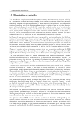
2.4 Evolutionary algorithms
The original mechanisms of evolution of the living beings rest on the competition
which selects the most well adapted individuals to their environment while ensuring
a descent, as in the transmission of the useful characteristics to the children which
allowed the survival of the parents. — C. Darwin [19]
Evolutionary computations are stochastic search techniques that imitate the genetic evolutionary
process of species based on the Darwinian concepts of natural selection and survival of the fittest.
That is, in nature, evolution occurs as a result of the competition among individuals for scarce
resources, resulting in the fittest individuals dominating the weaker ones. Those individuals
best adapted for survival are selected for reproduction in order to ensure that strong, useful
genetic material is transmitted to their offspring, thus promoting the continuation of the species
[24, 48]. A genetic algorithm is a population-based metaheuristic in the class of evolutionary
algorithms which operates analogously to the concept of evolution via natural selection. This
algorithm was first introduced by Holland [68] in 1975 in an attempt to understand the (then
not-so-popular) mechanisms of self-adaptive systems.
2.4.1 Algorithm outline
In a genetic algorithm, a population of individuals representing candidate solutions to an op-
timisation problem is iteratively evolved toward better solutions. A fitness function measures
the performance of a candidate solution or individual, and is a quantisation of its desirability of
being selected for propagation. Each individual is genetically represented by a set of chromo-
somes (or a genome) made up of genes which may take on a certain range of values from some
genetic domain, known as alleles. The position of a gene within its chromosome is identified by
means of a locus. The population evolves in an iterative manner over a certain number of gen-
erations until a stopping criterion is met. Individuals are represented as strings corresponding
to a biological genotype (encoded), which defines an individual organism when it is expressed as
a phenotype (decoded).
Inspired by nature, genetic algorithms attempt to improve the population of individuals at
every generation through repetitive application of a range of genetic operators. During every
generation, a proportion of parent solutions from the current population is chosen to produce
a new generation of offspring solutions. Parent solutions are selected for reproduction through
a fitness-based process called selection in such a manner that fitter solutions have a higher
probability of being selected to reproduce. Offspring solutions are generated via a combination
of two operators, namely a crossover operator, which exchanges genetic material in the form of
chromosome sub-strings of a pair of parent solutions to produce one or more offspring solutions
(analogous to the process of species reproduction in nature), and a mutation operator, which
alters a gene in the chromosome string of an offspring solution with a certain probability so
as to form a mutated individual. In addition, a replacement operator filters the individuals to
move on to the next generation so as to maintain a certain population size, after which the
entire process is repeated. Record is kept of the fittest individual found throughout the search,
which is again called the incumbent solution (similarly to the incumbent solution recorded in
the method of simulated annealing).
Populating the next generation mostly by means of new offspring solutions can, however, cause
the loss of the best individual(s) from the previous generation. To remedy to this disadvantage,
an elitism operator may be introduced, which ensures that at least one best solution from the](https://image.slidesharecdn.com/6cd1ebf5-5cfe-4d40-998c-99cbe17b08f1-170109122537/85/PhD-dissertation-59-320.jpg)
![28 Chapter 2. Literature Review
current parent population is retained (without changes) to the next generation, so that the
best solution(s) found throughout the algorithm can survive until the end. Examples of other
genetic operators include immigration, where one or more randomly generated solutions are
introduced into the population during every generation; education, where a local transformation
is intentionally conducted in respect of certain offspring solutions to try improve their fitness
prior to initiation of the selection process or to cure possible infeasibilities; and inbreeding, where
two highly fit offspring solutions generated from the same pair of parent solutions intentionally
reproduce with one another during the following generation.
Although genetic algorithms typically use a subset or variation of genetic operators, the general
concept nevertheless remains the same in all cases: genetic algorithms are motivated by the basic
idea that populations improve in a way that the average fitness of the population of solutions
generally increases during every generation, which consequently increases the chances of finding
a global optimum to the optimisation problem at hand after a large number of generations. A
flowchart of the general working of a genetic algorithm is presented in Figure 2.4, where only
the fundamental genetic operators are considered, and a pseudo-code description of the basic
steps featured in this kind of search is given in Algorithm 2.2.
Algorithm 2.2: Genetic algorithm outline
Generate initial population of individuals1
Evaluate the fitness of each individual2
while Stopping criterion not met do3
Select parent solutions for reproduction4
Generate offspring population5
Apply mutation operator to offspring solutions6
Evaluate fitness of offspring solutions7
Select individuals to be carried over to the next generation8
Update incumbent solution (if necessary)9
Report incumbent solution10
2.4.2 Multiobjective evolutionary algorithms
Like numerous other search techniques, multiobjective evolutionary algorithms were initially
designed as a means to find trade-offs between the objective performance measures of candidate
solutions. The overall benefits that evolutionary algorithms bring to multiobjective decision
making problems are today the reason for the growing interest of researchers in this field, in
particular with regard to their ability to generate several elements of the Pareto optimal set in a
single run [81]. It is believed that evolutionary algorithms and, in particular, genetic algorithms,
are so well suited for these types of problems as a result of their analogous connection to biological
processes exhibiting multiobjective features in nature. According to Zitzler et al. [167], two major
problems must be addressed when solving a multiobjective optimisation problem by means of a
genetic algorithm. One is to configure the fitness assignment and selection processes effectively
in order to guide the search towards the Pareto front, and the other is to maintain a diverse
population in order to prevent premature convergence and generate a good spread of solutions
along the approximate Pareto front.
During the period 1993–1995, researchers began in earnest to investigate the possibility of using
evolutionary algorithmic techniques for solving multiobjective optimisation problems. Among
these early approaches, the multiobjective genetic algorithm [105], the non-dominated sorting](https://image.slidesharecdn.com/6cd1ebf5-5cfe-4d40-998c-99cbe17b08f1-170109122537/85/PhD-dissertation-60-320.jpg)
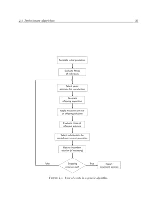
![30 Chapter 2. Literature Review
genetic algorithm (NSGA-I) [134] and the niched Pareto genetic algorithm [69] received partic-
ular attention. These algorithms were designed with the necessary additional components to
convert single objective evolutionary algorithms to multiobjective counterparts without the use
of weighting techniques, which often induce inconsistencies. Moreover, they are able to solve
problems in multidimentional objective space and generate multiple non-dominated solutions
near/along the Pareto front in a single run for a wide variety of optimisation problems. In gen-
eral, two fundamental features are found in such techniques: (1) the assignment of fitness values
to population individuals based on non-dominated sorting and (2) the preservation of diversity
among solutions located on the same non-dominated front.
Researchers have, however, realised that, although the above-mentioned approaches are per-
haps surprisingly effective in finding non-dominated solutions for many test problems, a wider
variety of operators than mere crossover and mutation are required to improve computational
performance. For example, elitism was introduced in an attempt to improve the convergence
properties of the algorithms and to prevent the extinction of good solutions once they have been
uncovered. The suggestion to include elitism was indeed a good one, as it has been shown that
multiobjective evolutionary algorithms are subsequently able to achieve better converging prop-
erties [167], and are generally able to find non-dominated solutions faster. The strength Pareto
evolutionary algorithm [169] and the Pareto archived evolution strategy [79], in particular, are
popular multiobjective genetic algorithm techniques which make use of the notion of elitism.
The NSGA-I mentioned above was one of the very first multiobjective evolutionary algorithms to
function without the use of user-defined objective preference weights (which amounts to solving a
multiobjective problem in uni-dimensional objective space). In other words, the non-dominated
population of the last generation represents an approximation of the Pareto-optimal set, from
which a compromise solution may be chosen at the discretion of the decision maker. During the
1990s, the performance level of this algorithm was very high relative to the alternative, more
traditional methods then available. Continual research in the field of multiobjective evolutionary
algorithms over time, however, allowed for the discovery of shortcomings in the method. More
specifically, three important criticisms were raised. The first had to do with the high computa-
tional complexity of the NSGA-I. Implementation of the algorithm is computationally expensive
for large population sizes, particularly due to the complexity associated with its non-dominated
sorting procedure, which has to be performed at every generation. Secondly, the NSGA-I lacked
the incorporation of elitism. As mentioned earlier, not only does elitism improve the convergence
rate of the algorithm, it also prevents the loss of good solutions once they have been uncovered.
Lastly, it was argued that the NSGA-I requires an additional parameter for a more effective
diversity-preservation mechanism. In particular, the NSGA-I incorporated a so-called sharing
parameter to this effect, which may be thought of as the distance metric chosen to calculate a
proximity measure between two individuals in the current population. However, the addition of
such a parameter raises two main complications. First, the performance of the sharing function
in terms of maintaining a good spread of solutions relies too heavily on the parameter value
chosen (which is user-defined). Secondly, according to this diversity preservation mechanism,
every solution in the current population must be compared with every other solution, which
may dramatically increase the problem complexity when the size of the population is large (in
addition to the complexity associated with the non-dominated sorting procedure pointed out
above).
Seven years later, Deb et al. [41] developed an improved version of the original NSGA-I, and
called it the NSGA-II. Their method incorporates a better sorting algorithm, allows for elitism,
and does not require the user to define a sharing parameter a priori, hence addressing all of the
disadvantages raised in respect of the original NSGA-I. Perhaps the main difference between](https://image.slidesharecdn.com/6cd1ebf5-5cfe-4d40-998c-99cbe17b08f1-170109122537/85/PhD-dissertation-62-320.jpg)
![2.4. Evolutionary algorithms 31
the two algorithm versions is that, while the fitness of a candidate solution in the NSGA-
I is evaluated using non-dominated sorting only, the NSGA-II makes use of non-dominated
sorting as well as diversity preservation in order to assess the fitness of individuals. Moreover,
it has been demonstrated that the NSGA-II outperforms two other successful multiobjective
evolutionary algorithms (namely the Strength Pareto Evolutionary Algorithm and the Pareto
Archived Evolution Strategy) on the grounds of not only finding a more diverse set of candidate
solutions but also in achieving convergence in close proximity to the true Pareto-optimal set for
a wide variety of problems.
Overall, multiobjective evolutionary algorithms generally share certain fundamental common
features. Their differences are not as complex as one might expect; they are often just individ-
ually designed incarnations of the same basic principle achieved in a unique, creative manner.
According to Coello et al. [29], the generic goals and operator design of all these algorithmic
variations are (1) to preserve non-dominated points in objective space and respective solution
points in decision space, (2) to continue to make algorithmic progress toward the Pareto front in
objective space, (3) to maintain diversity among the points on or near the Pareto front, and (4)
to provide the decision maker with a sufficient, but not overwhelming number of non-dominated
points for alternative selection.
2.4.3 Fitness assignment and diversity preservation
As previously discussed, one goal in multiobjective evolutionary optimisation is to ensure that
higher quality individuals have a greater chance of being selected to pass their genetic material
on to the next generation. Moreover, it was mentioned in §2.4.1 that the quality of a solution
in a genetic algorithm is assessed by its fitness level. In single-objective optimisation problems,
the fitness values of individuals are typically assessed on a uni-dimensional continuum, where
individuals with higher fitness values are deemed more desirable. In multiobjective optimisation
problems, however, the notion of dominance (see §2.1.4) is typically used to assess the fitness
of individuals (such fitness measures are thus represented as cardinal numbers), in contrast to
single-objective optimisation problems, where the fitness of a solution is purely based on its
objective function value along the real number line. Perhaps the two most popular dominance
criteria used in the design of a fitness measure in multiobjective genetic algorithms are dominance
strength, which represents the number of solutions that a particular individual dominates in a
population, and dominance count, which is the number of solutions in the population that
dominate a particular individual solution [120].
Another goal in multiobjective evolutionary optimisation is to maintain diversity among pop-
ulation members. This may be achieved by considering the density of individual solutions in
objective space, in the sense that solutions in less crowded regions are favoured to be selected for
reproduction and/or carried over to the next generation in an attempt to stimulate exploration
of unexplored regions of the search space. Restricted mating, crowding distance and relaxed
domination are examples of popular diversity preservation measures [120].
2.4.4 Genetic operators
A brief overview of some fundamental genetic algorithm operators, namely selection, crossover
and mutation, is presented in this section. Because these operators are applicable to both single
and multiobjective problems, no differentiation is made between these two classes of optimisation
problems in this section.](https://image.slidesharecdn.com/6cd1ebf5-5cfe-4d40-998c-99cbe17b08f1-170109122537/85/PhD-dissertation-63-320.jpg)
![32 Chapter 2. Literature Review
Selection operators
Selection refers to the process of selecting parent solutions from a population based primarily on
their fitness values and, secondarily on their relative density values, to form a mating pool from
which offspring solutions are created. In evolutionary algorithms, selective pressure is a term
widely used to characterise the high emphasis on selection of the best individuals [3]. Selection
pressure may be interpreted as the driving force behind improving the average population fitness
over the course of generations which, in turn, has an impact on the convergence properties of the
algorithm. Because selection is completely independent of the remaining operators applied in
the algorithm, it may be characterised as a universal, problem-independent, operator. According
to Back [3], the impact of the control parameters on the selection pressure should be simple and
predictable to some extent. Additionally, a single parameter is preferred for the implementation
of selective pressure, and the range of selective pressure that may be achieved by varying this
control parameter should be as large as possible.
Many types of selection operators are described in the literature, all essentially with the single
collective purpose of selecting individuals from the population in a probabilistic manner and
inserting them in the mating pool. Examples of selection operators which may be employed
in evolutionary algorithms include fitness proportion selection (also known as roulette wheel
selection), where the probability of an individual being selected is simply assessed as the quotient
of its fitness level and the sum of the fitness levels of all individuals in the population; stochastic
universal sampling, where weaker individuals are given a fairer chance of being selected than in
fitness proportion selection; tournament selection, where a certain number of individuals chosen
at random from the population compete with one another in terms of fitness levels from whence
a victor is selected8; and truncation selection, where the population members are ranked by
fitness, and a certain proportion of the fittest individuals are all selected, each to reproduce
a certain number of times. The interested reader is referred to [81] for a description on the
workings of these selection procedures.
Crossover operators
The crossover genetic operator combines the chromosomes of two parent solutions in order to
produce one or more offspring solutions. The motivation behind the use of this operator is that
an offspring solution might turn out better than both of its parents if it acquires good sets of
genes from each of them. There exist many types of crossover operators in the literature, and
the type of operator to be implemented depends mostly on the type of optimisation problem at
hand and, in particular, on the nature of the solution representation scheme adopted.
Examples of crossover operators which may be employed include single point crossover, in which
all genetic data beyond the crossover point in each chromosome string is swapped between the
two strings; two-point crossover, in which all genetic material between two crossover points in
each chromosome string is swapped between the two strings; cut-and-splice crossover, in which
each parent solution has a separate crossover point, causing the resulting offspring chromosome
strings to vary in size; and uniform crossover, which may be viewed as a multipoint crossover in
which the number of crossover points is unspecified a priori. The interested reader is referred to
[81] for a more thorough description on the workings of these crossover procedures. Graphical
illustrations of the first three crossover operators listed above may be found in Figure 2.5 for
the case where the chromosome strings are represented as binary coded genotypes.
8
With tournament selection, selection pressure is adjusted by altering the tournament size, where a larger
tournament size affords weaker individuals a lower chance of being selected.](https://image.slidesharecdn.com/6cd1ebf5-5cfe-4d40-998c-99cbe17b08f1-170109122537/85/PhD-dissertation-64-320.jpg)
![2.4. Evolutionary algorithms 33
1 1 0 0 1 0 1 1
Parent 1 genotype
0 1 1 0 1 0 1 0
Parent 2 genotype
1 1 0 0 1 0 1 0
Offspring 1 genotype
0 1 1 0 1 0 1 1
Offspring 2 genotype
(a) Single point crossover.
1 1 0 0 1 0 1 1
Parent 1 genotype
0 1 1 0 1 0 1 0
Parent 2 genotype
1 1 1 0 1 0 1 1
Offspring 1 genotype
0 1 0 0 1 0 1 0
Offspring 2 genotype
(b) Two-point crossover.
1 1 0 0 1 0 1 1
Parent 1 genotype
0 1 1 0 1 0 1 0
Parent 2 genotype
1 1 0 0 1 1 0
Offspring 1 genotype
0 1 1 0 1 0 0 1 1
Offspring 2 genotype
(c) Cut-and-splice crossover.
Figure 2.5: Illustration of three popular crossover procedures in the literature.
Mutation operators
The individuals having the best fitnesses are reproduced more often than the others
and replace the worst ones. If the variation operators are inhibited, the best individual
should reproduce more quickly than the others, until its copies completely take over
the population. — J. Dr´eo [48]
Mutation is often considered a minor operator in genetic algorithms. It is aimed at maintaining
a minimum level of diversity among population individuals, which the crossover operator may
perhaps not be able to ensure at all times, in an attempt to move the search toward unexplored
regions of the search space with the hope of finding high-quality solutions there. A mutation
operator typically modifies an offspring solution stochastically in such a way that the result of
the transformation is close to its original chromosome form (i.e. a local search is performed). The
proportion of mutated individuals in the offspring population is controlled using a mutation rate
parameter. A mutation operator with a significantly high mutation rate is expected to produce
the desired results in terms of preservation of diversity, particularly in respect of preventing
population individuals from becoming too similar to one another. As a result, it is expected to
slow down the evolution progress to a certain extent. Moreover, according to Dr´eo [48], mutations
may be particularly useful for significantly improving the quality of solutions discovered when
most of the population is located in the neighbourhood of a global optimum or Pareto front
(whereas the importance of the crossover operator diminishes once the population reaches that
stage in the algorithm), provided that the mutation rate is high enough. Setting the mutation](https://image.slidesharecdn.com/6cd1ebf5-5cfe-4d40-998c-99cbe17b08f1-170109122537/85/PhD-dissertation-65-320.jpg)
![34 Chapter 2. Literature Review
rate too high, however, may result in individuals being produced almost independently from
the genetic material passed on to them from their parents, which may cause the algorithmic
progress to mimic a collection of primitive random walks in the solution space.
Mutation is typically performed by altering the state of a gene in a chromosome string according
to a certain probability, which is obtained from the mutation rate parameter. As with crossover
operators, the type of mutation operator to be implemented depends mostly on the type of opti-
misation problem at hand. Examples of mutation operators which may be employed include bit
string mutation, where alleles of binary coded genotypes are each altered according to a certain
probability based on the length of the chromosome string and the mutation rate; boundary mu-
tation, where alleles are replaced by either one of user-defined upper or lower bounds according
to a certain probability; uniform mutation, where alleles are replaced by a uniform random
value selected between user-defined bounds according to a certain probability; and non-uniform
mutation, where the mutation rate is altered throughout the algorithm in order to prevent the
population from stagnating during the early stages of evolution while increasing the expected
number of mutated offspring solutions during later stages of the process. An example of bit
string mutation is shown in Figure 2.6. The interested reader is referred to [81] for a more
detailed description of the workings of the mutation operators mentioned above.
1 1 0 0 1 1 0 1
Pre-mutated genotype
1 1 0 0 1 0 0 1
Post-mutated genotype
Figure 2.6: Illustration of a bit string mutation operator.
2.5 Other popular metaheuristics
In this section, three other popular metaheuristics are briefly discussed for single objective
optimisation problems, namely the methods of tabu search, ant colony optimisation and particle
swarm optimisation. Unlike the previous two sections, in which detailed algorithmic descriptions
were provided, the purpose of this section is rather to describe the conceptual ideas behind
these innovative search techniques in order to provide more insight into three modern, high-
performance metaheuristics.
2.5.1 The method of tabu search
Tabu search is primarily a deterministic local search method which is based on the idea that
a short-term memory component should be used during the exploration of the neighbourhood
around a candidate solution in an optimisation problem. The goal of incorporating such a
memory component in the search is to prohibit it from periodically returning to recently visited
solutions and, in particular, to avoid the search from revisiting local optima [48].
The local search process conducted in a tabu search evolves around the neighbourhood set N(x)
of a solution x. This set contains all feasible solutions obtainable from x by applying a move
from a so-called move set. This move set traditionally consists of a finite number of solution
transformation methods. In general, however, a tabu search does not need to evaluate the full
neighbourhood set of a solution when this set is large9, but is rather expected to make an
9
In contrast, the method of simulated annealing only considers one neighbouring solution at every iteration.](https://image.slidesharecdn.com/6cd1ebf5-5cfe-4d40-998c-99cbe17b08f1-170109122537/85/PhD-dissertation-66-320.jpg)
![2.5. Other popular metaheuristics 35
intelligent choice with respect to the nature of the generated neighbourhood set. Hence, the
purpose of a move set is to reduce the size of the neighbourhood around a solution in order
to prevent the search from visiting neighbouring solutions not worth visiting. Alternatively,
restrictions may be imposed on move instances, rather than specific solutions, whose reversals
are thereby forbidden. A strong tabu search is therefore required to include, amongst other
aspects, an effective local search mechanism. In particular, the relationship between the quality
of the move set, the types of moves and the computational budget necessary for their evaluation
in objective space, ought to be configured in the correct manner.
Following the creation of a neighbourhood set around a current solution, the best solution within
that set is then selected as the new current solution. To prevent the search from revisiting a
recent solution, a tabu list T is maintained which keeps track of the |T | previously visited
solutions, called tabu solutions. These solutions are excluded from the neighbourhood set of the
current solution as long as they remain members of the tabu list. This list is usually managed to
maintain a fixed length in a first-in-first-out fashion, after which tabu solutions removed from
the list are relabelled as non-tabu. There exist several stopping criteria that may be employed
to terminate the algorithm.
A flowchart of the working of the method of tabu search is presented in Figure 2.7. In addition,
a pseudo-code description of the basic steps featured in a tabu search is given in Algorithm 2.3.
In line 8 of the pseudo-code, the previous solution is added to the head of the tabu list, while
the solution at the tail of the list is reclassified as being non-tabu, provided that the list has
already reached its full capacity (if that is not the case, then the tail in this list may be thought
of as an empty slot).
Algorithm 2.3: Tabu search algorithm outline
Generate initial feasible solution1
Set tabu list T ← ∅2
while Stopping criterion not met do3
Generate current solution neighbourhood N(x)4
Evaluate the performance of non-tabu solutions in N(x)5
Select best neighbour solution x∗6
Update incumbent solution (if necessary)7
Update tabu list T ← {T T (|T |)} ∪ x8
Set new current solution x ← x∗9
Report incumbent solution10
2.5.2 Ant colony optimisation
The method of ant colony optimisation is a so-called self-organisation metaheuristic naturally
inspired by the collective behaviour of ants whilst seeking food sources. In nature, a colony of
ants communicate indirectly with one another via ground trails of odorous volatile substances,
known as pheromones [48]. The ants collectively use these trails to indicate desired channels
between their nest and a food source for exploitation, enabling the colony to ultimately assess
an optimal path towards the source without requiring individual ants to have a global pattern
overview (i.e. only local information is utilised by the ants). These indirect social interactions
by means of modifications of the environment is better known as stigmergy in biological studies.
A trail containing a higher concentration of pheromones is deemed more desirable and has](https://image.slidesharecdn.com/6cd1ebf5-5cfe-4d40-998c-99cbe17b08f1-170109122537/85/PhD-dissertation-67-320.jpg)
![36 Chapter 2. Literature Review
Generate initial solution
Set tabu list T ← ∅
Generate current
solution neighbourhood
Evaluate the performance
of non-tabu solutions in the
generated neighbourhood
Select best
neighbouring solution
Update incumbent
solution (if necessary)
Stopping
criterion met?
Update tabu list
False
Set new
current solution
Report
incumbent solution
True
Figure 2.7: Flow of operations in the method of tabu search.
a higher probability of being traversed by any given ant. In addition, the natural chemical
constitution of pheromone levels causes these trails to evaporate over time, unless other ants
re-traverse the trails and deposit more pheromones onto them. This is a necessary phenomenon
in the process as it allows the system to “forget poor solutions” and avoid being trapped at
local optima. The concentration of pheromones along a certain trail is therefore an indication
of the volume of ant traffic on that trail. As a result, the path with the highest concentration of
pheromones (typically the shortest path) will be chosen by the majority of ants in the long run
until the food source expires. This method has proven to be very popular for solving variants
of the travelling salesman problem (which initially motivated the design of the method of ant
colony optimisation by Dorigo and Gambardella [47] in 1997), as well as routing and graph
colouring problems later on.
An ant colony system may be modelled as a complete graph G(V, E) with a set V of nodes and
a set E of edges inter-linking all pairs of these nodes, where each ant a in a set of ants traverses
the graph and builds a pheromone trail at every iteration t ∈ {1, . . . , tmax} of the process. Each
edge is initially assigned a certain pheromone concentration. For each ant at any given node
i ∈ V, the selection of the edge between node i and node j is determined by three factors, namely
the list Jai of remaining nodes to be visited by ant a provided that it is currently at node i,](https://image.slidesharecdn.com/6cd1ebf5-5cfe-4d40-998c-99cbe17b08f1-170109122537/85/PhD-dissertation-68-320.jpg)
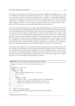
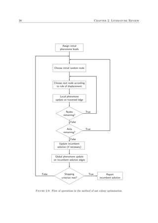
![2.6. The vehicle routing problem 39
2.5.3 Particle swarm optimisation
The method of partical swarm optimisation is a population-based metaheuristic which was orig-
inally based on the socio-psychological principles emanating from the collective behaviour of
decentralised, self-organised agents [76, 114]. Unlike evolutionary algorithms, particle swarm
optimisation does not make use of selection and reproduction operators. Instead, all popula-
tion members survive throughout the algorithm (as is the case in ant colony optimisation) and
their interactions mainly evolve around the iterative improvement of solutions over time. The
initial idea behind swarm intelligence was presented by Eberhart and Kennedy [50] in 1995,
who attempted to produce computational intelligence by exploiting certain analogues of so-
cial interaction, rather than purely being individual-based like most other metaheuristic search
techniques.
In the method of particle swarm optimisation, a population of particles is initially individually
placed at random locations in the solution space of some optimisation problem, and are evaluated
in objective space. Each particle in the swarm S then follows a path through the solution space.
This path is determined by combining its current and historically best locations (“best” with
respect to the performance of that location in objective space) with those of one or more other
particles in the swarm, as well as allowing for random perturbations.
At every iteration, each particle p is moved one step further from its current location p according
to a certain velocity vector pv. The coordinates of pv are added to the coordinates of p to
determine the new location of the particle. The best location p ∗ found thus far during the
search for a specific particle is updated at every iteration. In addition, the best location N(p) ∗
found thus during the search in the neighbourhood of a specific particle is tracked by the particle
swarm optimiser. Finally, an incumbent solution representing the best location found thus far
by the entire swarm is also archived (i.e. the best location found when any particle takes all
swarm particles as its topological neighbours). The particle swarm optimisation concept consists
of tuning the velocity vector of each particle toward N(p) ∗ and toward the incumbent solution
at every iteration. This sudden change in velocity is magnified by random terms generated for
accelerating particles toward these locations [165].
The swarm is more than just a collection of particle solutions. A particle by itself has almost
no power to influence the search direction; improvement in the search only occurs when the
particles interact with one another. The idea is that, similarly to a flock of birds seeking food
sources, the swarm will eventually approach a global optimum of the optimisation problem at
hand. A flowchart of the working of the method of particle swarm optimisation is presented in
Figure 2.9 and a pseudo-code description of the basic steps featured in this method is given in
Algorithm 2.5.
2.6 The vehicle routing problem
The VRP is considered one of the most important and complex combinatorial optimisation
problems in the operations research literature. It is easy to describe, but very difficult to solve
[135], and is itself a combination of two other celebrated combinatorial optimisation problems,
namely the bin packing problem in which, given the capacity of a bin and a finite set of items
of specific sizes, the minimum number of bins required to contain all the items is sought, and
the travelling salesman problem in which, given a weighted complete graph, a shortest closed
tour including every node in the graph is sought. Perhaps the most appealing feature of the
VRP is that its original formulation, known as the capacitated VRP, may be extended to nu-](https://image.slidesharecdn.com/6cd1ebf5-5cfe-4d40-998c-99cbe17b08f1-170109122537/85/PhD-dissertation-71-320.jpg)
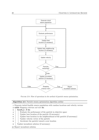
![2.6. The vehicle routing problem 41
merous variations for solving a variety of real-world routing problems. This section contains a
brief review on the origin and variation of VRPs, and this is followed by a discussion on the
nature of specific problem information associated with VRPs. In this discussion, dynamic and
stochastic VRPs are afforded special attention. Additionally, a specialised review of solution
search methodologies for VRPs related to the MLE response selection problem is conducted.
2.6.1 The origin and variations of the problem
The first description of the VRP was given by Dantzig and Ramser [37] in 1959 in a paper called
the Truck dispatching problem. The reason for investigating this type of problem was to propose
a generalisation of the travelling salesman problem in which the salesman is required to return
to his starting point after visiting a certain number of customers. In generic terms, the problem
was to find a shortest set of tours which together pass through all vertices of a weighted complete
graph such that all tours contain a pre-defined, single point (called the depot) in common and
the total tour length is a minimum. A real-life problem involving the optimal routing of a fleet of
fuel delivery trucks between a fuel depot and a large number of petrol service stations supplied
by the depot was then formulated in the 1959 paper of Dantzig and Ramser [37], in which it was
assumed that information related to the shortest path between any two nodes in the set of petrol
service stations and the fuel demand of each station are known a priori. In this scenario, each
petrol station was required to be visited exactly once by a single delivery truck, and no truck’s
cargo was allowed to exceed its pre-determined capacity. Moreover, the routing was to occur in
such a way that the fuel demand quantities are all met and such that the total distance covered
by the fleet of trucks is a minimum. A procedure based on a linear programming formulation
for obtaining a near-optimal solution was proposed as an approximate approach toward solving
this problem.
This method, however, has a significant shortcoming with respect to satisfying the minimisation
of total routing costs. Indeed, according to this procedure, the distribution routes are prioritised
based on the combined demands of a set of customers relative to a certain fraction expressed in
terms of the capacity of the vehicle in use and the total number of customers to be served in
the system. In other words, the procedure places more emphasis on filling the trucks as close
to their full capacities as possible rather than on minimising the overall distance covered by the
fleet10. As a result, it is possible for customers located far from each other to be assigned to the
same route without any form of penalties.
In 1964, Clarke and Wright [26] published a paper introducing an effective greedy heuristic for
solving capacitated VRPs, which later became known as the Clarke-Wright algorithm. This
method iteratively forms routes by creating links between pairs of vertices, ranked according
to their savings in distance travelled, while maintaining feasibility. The real-life problem in
[37] was then solved using this heuristic in order to demonstrate its reasoning and evaluate its
performance. Despite consisting of only 30 customers, the Clarke-Wright algorithm generated
a 17% improvement in the objective function value of the problem over the former method by
Dantzig and Ramser [37].
Numerous algorithms and greedy heuristics have subsequently been published during the fifty
years following the publications of these two seminal papers, as the applications of the VRP
to real-life problems grew significantly during that period. Modifications to the capacitated
VRP model are routinely introduced in the literature in order to incorporate new, fundamental
aspects of some practical problem, such as VRPs with customer time windows, split deliveries,
10
In multiobjective VRPs, however, one might be interested in minimising the total distance travelled by the
fleet and to minimise the size of the fleet in service.](https://image.slidesharecdn.com/6cd1ebf5-5cfe-4d40-998c-99cbe17b08f1-170109122537/85/PhD-dissertation-73-320.jpg)
![42 Chapter 2. Literature Review
multiple depots, heterogeneous fleets of vehicles, customer profits, asymmetric travel arcs, demand
ranges, etc. The interested reader is referred to the authoritative book by Toth and Vigo [150]
for generic formulations of these VRP variants. Many papers also focus on in-depth theoretical
analyses of these problems, often putting forward effective search techniques for solving them.
Smaller studies have also focused on niched practical aspects of variations on the VRP, such
as simulating the impact of service lead time on the costs of deliveries from a centralised fuel
depot with a homogeneous fleet of vehicles in a medium-scale, semi-rural environment [34]. In
most real-life VRP applications, the problem to be solved is very specific. It is therefore critical
to achieve a good understanding of the specifics of the problem at hand, and also of the VRP
variants and associated optimisation techniques available in the literature, in order to describe,
model and solve the problem in an appropriate and effective manner.
2.6.2 The nature of specific problem information
According to Psaraftis [118], real-world applications of VRP formulations may be classified ac-
cording to four attributes of the nature of information required to specify problem instances,
namely the evolution, quality, availability and processing of information. The nature of infor-
mation in a VRP plays a critical role in the characterisation, modelling and solution search
methodology that should be adopted. These attributes, together with their respective values,
are shown in Table 2.1.
In the above discussion, the evolution of information refers to the information available to the
decision maker during the execution of vehicle routes, which may either be classified as static
(where the input data are known for the entire duration of the routing process and are not subject
to any updates), or dynamic (where the input data are not known for the entire duration of the
routing process, but are generally revealed or updated as time passes). The quality of information
refers to possible uncertainty in respect of the available input data, which may either be classified
as deterministic (where the input data are known with certainty once made available), forecasts
(where the input data are subject to revisions as the process evolves), stochastic (where certain
input data are prescribed as probability distributions or evolve according to certain stochastic
processes), or unknown. The availability of information may either be classified as local (where
only certain role players in the routing process are immediately made aware of changes in input
data), or global (where changes in input data are updated continuously to most or all role
players). Finally, the processing of information refers to two main paradigms in respect of the
processes followed once new information is made available, which may be classified as either
centralised (where all information is collected and processed by a central unit), or decentralised
(where some of the information is processed separately from the central unit).
Evolution Quality Availability Processing
Static Deterministic Local Centralised
Dynamic Forecasts Global Decentralised
Stochastic
Unknown
Table 2.1: Classification of VRPs with respect to the nature of specific problem information [118].](https://image.slidesharecdn.com/6cd1ebf5-5cfe-4d40-998c-99cbe17b08f1-170109122537/85/PhD-dissertation-74-320.jpg)
![2.6. The vehicle routing problem 43
2.6.3 Dynamic VRPs
As mentioned in the previous section, a VRP is said to be dynamic if input data to the problem
are made known to the decision maker in a continual fashion and are updated concurrently
with the determination of the set of routes. The decision maker is therefore required to solve
the problem in a sequential fashion; that is, to solve part of the problem on the basis of the
information already available, and then to resolve parts of the problem as new input data are
revealed. What distinguishes most modern VRP variants today (particularly in the context of
commodity distribution) from their past counterparts is that information used to determine the
nature of the routes is today typically continually revealed to the decision maker as a result of
revolutionary advances in information and communication technologies [118]. This advancement
in the role that information plays in VRP-related systems, together with the significant increase
in computing power at relatively low costs, makes it possible for large amounts of input data to
be updated in real time.
In contrast to their static counterparts, dynamic VRPs introduce new model aspects and chal-
lenges that increase the complexity of the decision making process as well as the assessment of
the overall performance of a given routing strategy. It is, for example, more likely that certain
customer requests may be rejected at any given time in a dynamic VRP because of the compli-
cation and costs associated with serving them on short notice, particularly with respect to the
locations of the vehicles in space at that time. Moreover, the ability to redirect an active vehicle
to a new route generally allows for cost savings. Dynamic VRPs are also known to increase the
set size of the objective functions in a model. For example, whereas the common objective in
static VRPs is to minimise routing costs, dynamic VRPs are more likely to introduce subsidiary
objectives such as service levels, throughput achievement, revenue maximisation or minimisation
of the overall delay between the placements and servicing of new orders [113].
Dynamic VRPs require making decisions in which a compromise or trade-off is sought between
the speed of generating a solution and the overall solution quality; that is, the time invested
in searching for good decisions comes at the price of less reactiveness to changes in the input
data [118]. This aspect is of particular importance in cases where customers are expected to be
serviced shortly after placing an order, and where a good decision must consequently be made as
fast as possible. In terms of performance, it is therefore critical to design a model and identify an
appropriate search technique that produces satisfactory solutions shortly after having received
a significant update in input data.
Some dynamic VRP methodologies also account for simplifying the complexity associated with
revisiting the decision making process at deterministic points in time by making use of pre-
defined time frames to bound the time dedicated to each problem instance in the form of a
sequence of static VRPs [113]. This approach may significantly reduce stress levels on the
decision maker as he is only required to perform a decision making process at known, evenly (or
appropriately) spread, points in time. Additionally, it potentially allows more time for finding a
better solution to each problem instance (provided that the time frames are large enough). This
kind of dynamic VRP methodology is therefore effective for solving VRPs in which customer
orders are not subject to a high degree of urgency straight after they have been placed (i.e.
where a long lead time is allowed), or where there exists no objective function for minimising
the combined customer service delay time. The solution strategy proposed in [101], for example,
divides a working day into a fixed number of time slices of equal lengths. The input data
associated with the processing of new orders (which are generated stochastically in time) which
fall within a specific time slice are postponed to the beginning of the following time slice. The
decision maker then resolves the problem at the beginning of every time slice by computing a](https://image.slidesharecdn.com/6cd1ebf5-5cfe-4d40-998c-99cbe17b08f1-170109122537/85/PhD-dissertation-75-320.jpg)
![44 Chapter 2. Literature Review
new set of routes using the input data accumulated during the course of the previous time slice
in addition to the (known and still applicable) data gathered prior to that time slice over the
course of the working day.
2.6.4 Stochastic VRPs
As mentioned earlier, VRPs in which certain input data are prescribed as probability distribu-
tions (i.e. whenever one or more of the model parameters take the form of random variables), or
evolve with respect to certain stochastic processes, are said to be stochastic. In the literature,
VRPs of this type often tend to focus on the management of stochastic input data in such a way
as to minimise expected costs of routing operations (in the case of VRPs with stochastic travel
distances and/or travel times [83]), minimise expected delivery shortages (in the case of VRPs
with stochastic customer demands [64]) and preventing vehicle autonomy route failures11. Such
planning therefore typically involves designing routes in an economical fashion before actual
customer demands become known while minimising the overall probability of route failures.
In stochastic VRPs, unforeseen consequences manifested in real time typically lead to an increase
in expenses, both directly and indirectly. In particular, a trade-off exists between the savings in
travel costs due to larger routes and the frequency of route failures [136]. These expenses are
typically triggered in the form of additional vehicles dispatched to complete unfinished routes,
extra-time remuneration of drivers as a result of autonomy failures, customer dissatisfaction due
to poor service (where certain customers were never serviced or only partially serviced), waste
of time associated with loading and unloading vehicle shipments which were not delivered and
waste of fuel caused by vehicles travelling with undelivered (and thus unnecessary) loads.
Two general mathematical modelling approaches are found in the literature of stochastic VRPs
(and, in fact, in any stochastic programming problems). The first of these approaches is chance
constrained programming, where the objective function is to minimise planned route costs while
ensuring that having a route duration/distance in excess of the assigned vehicle’s time/distance
autonomy does not exceed a predetermined threshold. The second approach is stochastic pro-
gramming with recourse, where the cost of repairing a violated constrained to feasibility is
directly considered in the problem formulation, and where the objective function consists in
minimising the expected routing costs as well as the penalty costs associated with violated con-
straints. While chance constrained programming is relatively more appealing and easier to use,
stochastic programming with recourse is able to take the expected costs related to excess route
durations into account as well as in proportion to the extent of excess. In one of the recourse
models proposed for the VRP with stochastic travel times by Laporte et al. [83], for example, the
vehicles incur a routing penalty which is directly proportional to the duration of their respective
routes in excess of a (preset) fixed time parameter.
2.6.5 VRP solution methodologies in the literature
Due to their simplicity and fast computations, VRP heuristics are very popular for obtaining sat-
isfactory, though only approximately Pareto-optimal, solutions to small-scale problem instances.
Solving large-scale VRP instances with multiple complex objectives is, however, very difficult
using only heuristic techniques if the goal is to attain a good approximation of the Pareto front.
VRPs of this nature call for the use of alternative, more powerful solution search techniques.
11
A route failure is said to occur whenever the travel time and/or travel distance associated with a route
exceeds the assigned vehicle’s distance and/or time autonomy levels. Such a route is then said to be incomplete
or unfinished.](https://image.slidesharecdn.com/6cd1ebf5-5cfe-4d40-998c-99cbe17b08f1-170109122537/85/PhD-dissertation-76-320.jpg)
![2.6. The vehicle routing problem 45
There is consensus in the literature that VRPs are computationally very hard to solve, to the
point where instances of the capacitated, single-objective VRP (the most basic VRP formulation)
with 10 vehicles and more than 30–40 customers can only be solved approximately with the use of
metaheuristics [119]. Of course, this computational complexity typically increases when solving
more specialised VRP variants, such as solving VRPs with multiple depots in multiobjective
space. Moreover, VRPs with a heterogeneous fleet of vehicles are considered much harder to
solve than those with a homogeneous fleet [109].
The multi-depot VRP is a variant of the capacitated VRP in which routes are simultaneously
sought for several vehicles originating from multiple depots, serving a fixed set of customers
and then returning to their original depots. Compared to simpler VRPs and their variants, for
which abundant literature exists, only a relatively small volume of research has been done on
multi-depot VRPs. A small number of good optimisation techniques have nevertheless appeared
in the literature for this problem. Most of these techniques tend to break down an instance of
the problem into a series of single-depot sub-instances and/or only solve it for a single objective
and/or for a homogeneous fleet of vehicles [66, 67, 109, 140, 157]. Because vehicles always start
and complete their routes at the same depots, it is easy to merge the set of customer vertices
with that of the depot vertices in such simplified model formulations.
In [66] and [140], for example, the solution process for a single-objective, multi-depot VRP with
a homogeneous vehicle fleet is decomposed into a three-phase heuristic approach. The first phase
involves grouping the set of customers to be served by each depot (a clustering sub-problem),
while the second phase entails assigning customers served from the same depot to several routes
so that the capacity constraint associated with the vehicles is not violated (a routing sub-
problem). The third phase consists of determining the visitation sequence of customers located
on the same route (a scheduling sub-problem). The chief difference between considering multiple
depots simultaneously and solving multiple single-depot sub-problems separately is that the local
search operators in metaheuristics tailored to these approaches differ significantly in nature [157].
According to Salhi et al. [123], however, the decomposition of a multi-depot VRP into several
single-depot sub-problems by (naively) assigning the customers to the depots closest to them
(distance-wise), and solving these sub-problems individually, using a suitable approach, is easy
to carry out, but usually leads to poor, significantly sub-optimal solutions. As a result, the
mathematical modelling approach proposed in [123] is perhaps best suited to solving instances of
the MLE response selection problem in a centralised or intermediate decision making paradigm
(where the problem is solved globally). Salhi et al. [123] propose a complete mixed-integer,
linear formulation for a generic multi-depot VRP with a heterogeneous vehicle fleet. Moreover,
formulation variants are also offered for alternative VRP scenarios. For instance, multi-depot
VRP variants are considered in which the number of vehicles of a given type is known (i.e. a
heterogeneous fleet with defined classes of vehicles); in which certain types of vehicles cannot
be accommodated at certain depots; in which a vehicle is not required to return to the same
depot from whence it originated; or in which a maximum route length constraint associated
with each class of vehicle is imposed (i.e. a distance-constrained VRP). Salhi et al. [123] then
solve the problem (approximately) using a variable neighbourhood search applied to the notion
of borderline customers, using six different local search operators. Unfortunately, the model
formulation and search technique presented in [123] is applicable to single-objective optimisation
only. Consequently, it is unlikely that this variable neighbourhood search heuristic may be as
effective for solving similar problems in multiobjective space.
Many studies favour the use of genetic algorithms for solving the above-mentioned multiobjec-
tive VRP variants, often suggesting specific or unique genetic operators [66, 67, 88, 140, 157].
Moreover, due to the high complexity level associated with problems of this kind, many stud-](https://image.slidesharecdn.com/6cd1ebf5-5cfe-4d40-998c-99cbe17b08f1-170109122537/85/PhD-dissertation-77-320.jpg)
![46 Chapter 2. Literature Review
ies favour the use of hybrids over more traditional evolutionary computation approaches in an
attempt to improve algorithmic performance. The innovative hybrid genetic search with adap-
tive control proposed by Vidal et al. [157], for example, offers an optimisation methodology for
solving (among other problems), the multi-depot, periodic VRP with capacitated vehicles and
time windows. This hybrid includes a number of advanced features in terms of chromosome
fitness evaluation, offspring generation and improvement, and effective population management.
Two sub-populations are managed in [157] (one containing feasible individuals and the other
infeasible ones), and the mating pool is populated using parents from both sub-populations.
Furthermore, the selection operator mechanism takes into account both the fitness of individ-
uals and the level of contribution they provide to the diversity of the population. Offspring
solutions are enhanced fitness-wise using so-called education and repair local search procedures.
In [66], another hybrid genetic algorithm is proposed for solving difficult multi-depot VRPs.
Here, three external heuristics are combined with a traditional genetic algorithm to design a
hybrid between the Clarke-Wright algorithm [26], the nearest neighbour heuristic [145] and the
iterated swap procedure [86]. While the former two heuristics are solely used for generating
high-quality initial populations, the iterated swap procedure is applied to offspring solutions
which, if found to have better fitness values than one (or both) of their parents, replace that (or
those) parent solution(s) in the next generation of candidate solutions.
Although not as popular for solving complex multiobjective VRPs, certain authors have also
adopted traditional, sequential simulated annealing techniques as a means to finding solutions
to less complex VRPs [80, 87, 156, 164]. In these approaches, the very popular inter-route
and intra-route solution transformation techniques [156] are often used to provide the necessary
exploration and exploitation features to this metaheuristic for the purpose of generating a good
non-dominated front when tuned appropriately. Harnessing the processing power of parallel
computing has also been proposed for solving complex multiobjective VRPs [4].
Combining genetic algorithms with simulated annealing is not an uncommon strategy in the
literature for both single-objective and multiobjective optimisation VRPs [25, 108, 115, 128].
The hybrid proposed by Chen and Xu [25], for example, first employs the crossover and mutation
operations of genetic algorithms to produce offspring solutions, after which the fitness values
of the offspring solutions are evaluated, accepting offspring solutions in the next generation of
candidate solutions according to the Metropolis acceptance rule of simulated annealing.
Other metaheursitics employed in the literature for solving multiobjective VRPs include tabu
search, ant colony optimisation and particle swarm optimisation (see §2.5). Szymon and Dominik
[141], for instance, emphasise the value of using a parallel tabu search algorithm for solving a
multiobjective distance-constrained VRP. In [5], an ant colony system is put forward for solving a
tri-objective VRP in which it is required to minimise the number of vehicles used, the total travel
time and the overall delivery time. Finally, in [23], a particle swarm algorithm incorporating
certain features from multiobjective optimisation is used to allow particle solutions to conduct
a dynamic inter-objective trade-off in order to evolve seemingly poor infeasible routes to very
good ones using the benefits of swarm intelligence.
2.7 Dynamic multiobjective optimisation approaches
As discussed in §2.6.3, significant changes in one or more input parameters in a dynamic op-
timisation problem may cause the currently implemented solution to deteriorate significantly
in terms of quality and reliability. A decision maker must therefore solve part of the problem
on the basis of the information currently available, and then re-solve part of the problem as](https://image.slidesharecdn.com/6cd1ebf5-5cfe-4d40-998c-99cbe17b08f1-170109122537/85/PhD-dissertation-78-320.jpg)
![2.7. Dynamic multiobjective optimisation approaches 47
certain new input data are revealed and as fragments of the solution might no longer be feasible
or preferred. In this section, various approaches from the literature adopted in the context of
solving dynamic multiobjective optimisation problems are discussed in varying amount of detail.
2.7.1 On-line versus off-line optimisation
According to Deb et al. [40], one of two computational procedures is typically adopted for solv-
ing dynamic optimisation problems in general. In one procedure, optimal control laws or rules
are transformed over time by solving a so-called off-line optimisation problem, configured by
evaluating a given solution on a number of potential feasible scenarios to the dynamic problem.
The alternative procedure is known as on-line optimisation, where the (dynamic) problem is
considered stationary over a fixed period of time, and during which a solution search technique
is expected to seek an approximation set of the Pareto front. Thereafter, a new problem is con-
structed based on the current situation, following which a new optimisation process is conducted
during the new time period. Dynamic on-line optimisation problems can be classified further
into two subproblems in which the problem re-initialisation and optimisation procedures may
either occur at known, regular intervals in time, or may occur stochastically in time whenever a
significant change in the input data environment occurs.
While the off-line optimisation approach is typically useful in dynamic problems that are com-
putationally too complex for any algorithm to be applied in an on-line fashion, constructing and
finding appropriate control laws can, however, be a complex task and is very problem specific.
On the other hand, although much easier to implement than its off-line counterpart, the on-
line optimisation procedure may significantly be handicapped by the static consideration of the
problem during which the period of problem re-initialisation and optimisation procedures take
place, as the theoretical model upon which the domain space is defined may no longer be a true
and accurate representation of the present reality.
2.7.2 The notion of jump-start optimisation
It is often the case in many real-life dynamic problems that a certain level of urgency for
finding high-quality alternatives to high-complexity problem instances at certain points in time is
present. Although well adapted for static, once-off or sequential independent problem instances,
the various metaheuristics discussed so far in this chapter ultimately fail to capitalise on the
hidden benefits of domain space memory in the context of dynamic multiobjective optimisation
problems. In other words, these search techniques are only configured to treat every new problem
instance independently from the previous ones.
Unless changes in the domain space brought upon by input data alterations are very strong,
it has been demonstrated that significant computational effort may often be saved, and better
solution quality achieved, by reusing information gained in past problem instances when solving
dynamic multiobjective optimisation problems [20, 21, 40, 56]. In particular, it may often be
the case that any two consecutive feasible decision spaces in a dynamic multiobjective optimisa-
tion problem both contain identical subsets of solutions (provided that such solutions from the
previous problem instance are evolved in time accordingly). More importantly, it may be the
case that the intersection of any two consecutive Pareto optimal sets of solutions is significantly
large.
The notion of jump-start optimisation12 is the implementation of intelligent solution search
12
For lack of a unified term pertaining to this concept in the literature.](https://image.slidesharecdn.com/6cd1ebf5-5cfe-4d40-998c-99cbe17b08f1-170109122537/85/PhD-dissertation-79-320.jpg)
![48 Chapter 2. Literature Review
techniques that consider (to varying extents) a posteriori knowledge on the nature of the decision
and objective spaces configured during the previous problem instance at the start of the decision
making process accompanying a new problem instance. Additionally, jump-start optimisation
techniques may also be configured to track the shift in Pareto optimal solutions along the time
continuum of a dynamic multiobjective optimisation problem.
2.7.3 Adaptive evolutionary mechanisms
It is reasonable to expect that evolutionary algorithms may prove to be useful in dynamic
multiobjective problems, as they are inspired by a natural process that is subject to continu-
ous adaptation. In particular, the occurrences of major input data changes on a high-quality,
highly-diverse population of solutions in a dynamic multiobjective optimisation problem may,
analogously, be compared to the effect that local and global events have on the individuals of a
certain species (examples of such events include climatic changes, food sources depletion, natural
cataclysms, diseases and predators upsurge), and how these individuals are able to cope and
adapt to these events. Many studies therefore primarily focus on evolutionary techniques as a
means of adapting a solution search process to dynamic multiobjective optimisation problems
[12, 13, 20, 40, 74, 166].
In [40], for instance, various changes are performed on the original NSGA-II in order to adapt it
to dynamic multiobjective optimisation problems. This adaptive evolutionary algorithm was re-
named DNSGA-II. Due to a practical lack of consensus as to what level of input data variations
are deemed “significant”, this metaheuristic is not explicitly informed of all input data changes
that take place. Instead, a sub-loop is required to test whether a significant change has occurred
in the problem by selecting a few solutions at random from the current population and reevaluat-
ing them in both decision and objective space. If at least one change is observed amongst these
random individuals, all parent solutions in the current population undergo full reevaluation,
following which a new offspring population is generated. These two-subpopulations are then
merged into a new, more representative population. Moreover, two versions of the DNSGA-II
are presented in [40]. In the first version, a certain percentage of the newly adapted population
is replaced with random immigrants, which supposedly works better whenever changes in de-
cision and objective space are generally large. In the second version, instead of being replaced
by random immigrants, the selected percentage of population members undergo mutation, so
that the new solutions introduced into the new population are related to existing members of
the population. It is claimed that this approach generally works better for dynamic problems
in which small changes in input data generally take place.
According to C´amara et al. [21], an adaptive evolutionary optimisation tracking mechanism is
required to continuously maintain diversity and generate uniformly distributed solutions along
the non-dominated front as changes in the nature of the non-dominated objective space take
place. In addition, solution transformation procedures (such as mutation and crossover) should
ideally be set similarly to static problems, where an efficient trade-off is pursued between the
exploration of solutions in new areas and the general convergence toward better solutions in the
vicinity of the already good ones found.
In addition, Jin et al. [74] have stated in their research that diversity after the changes and di-
versity along the runtime are two very important notions that must be addressed in evolutionary
dynamic multiobjective optimisation problems. On the one hand, the notion of diversity after
the changes suggests that, as soon as a change in input data has been detected, diversity among
population members should temporary be increased in order to access new regions of the search
space and reassess the nature of the resulting new Pareto front. This is easily achievable using](https://image.slidesharecdn.com/6cd1ebf5-5cfe-4d40-998c-99cbe17b08f1-170109122537/85/PhD-dissertation-80-320.jpg)
![2.8. MLE DSSs in existence 49
a so-called hypermutation operator, where a sudden increment in the mutation rate is triggered
over a fixed computational period as soon as an observable change in input data has taken place.
On the other hand, the notion of diversity along the runtime suggests that close Pareto front
convergence throughout the execution of the algorithm (particularly during the early stages of
execution) should be avoided, so as to allow the algorithm to self-adapt and respond to the
changes more effectively. This adaptation process may be achieved by inserting random im-
migrants in the population once a certain number of generations has occurred. An even more
effective, yet more complicated, way to achieve this is to immigrate individuals exclusively to
the newly available feasible subregions of the search space.
Moreover, according to Cobb and Grefenstette [28], there exist two basic strategies for modifying
genetic algorithms to accommodate changing environments. The first strategy evolves around
expanding the memory space of the algorithm in order to build up a repertoire of ready responses
for pre-defined environmental conditions. The second strategy, similarly to that followed in [74],
is to employ some method for increasing diversity in the population (such as hypermutation) as
a means of compensating for changes encountered in the environment.
Finally, in the process of seeking non-dominated fronts throughout their adaptive evolutionary
algorithm, Farina et al. [56] have suggested that there exist four fundamental ways in which a
problem can demonstrate time-varying changes, namely (1) changes in Pareto optimal decision
variables (P) but not in the objective function mappings of Pareto optimal solutions (F), (2)
changes in both P and F, (3) changes in P but no changes in F and (4) no changes in either P
or F.
2.8 MLE DSSs in existence
Complex decisions made by system operators are usually supported to some extent by certain
automated assistance tools, better known in the literature as decision support systems (DSSs).
These tools aim to provide the operators with a set of high-quality alternatives in a limited time
for solving specific problem instances, particularly when dealing with decisions that are complex
and which are subject to a high level of uncertainty. This output may then be used in conjunction
with operator judgment (based on extensive knowledge, experience in the field and training) so
as to select a single, most preferred alternative for solving the problem at hand. A DSS does
not usually have the power to override operator decisions; the operator normally has the final
say in the outcome of the decision making process, although in extreme cases, the operator
may choose to implement one of the alternatives proposed by the DSS without contributing any
personal input to the decision process himself. On the other hand, if the problem complexity
is relatively low, the operator may simply prefer to make a subjective decision regardless of
the information provided by the DSS. In any case, alternatives proposed by a DSS should not
surprise an experienced operator, but rather confirm what he intuitively believes to be good
solutions to the problem at hand, as well as ease his conscience were he to experience some form
of doubt.
It is instructive to review some of the material presented in previous MLE-related research in
order to gain an understanding of certain aspects relevant to the scope of this dissertation.
Information related to the detection, evaluation and tracking of VOIs at sea provides most
of the essential input data for the MLE response selection process. These input data play a
critical role in the design of models for assessing the potentially threatening behaviour of VOIs
at sea and, as a result, many studies have been devoted to the processes of data collection, and
understanding and documenting the processes of threat detection, threat evaluation and vessel](https://image.slidesharecdn.com/6cd1ebf5-5cfe-4d40-998c-99cbe17b08f1-170109122537/85/PhD-dissertation-81-320.jpg)
![50 Chapter 2. Literature Review
tracking [9, 49, 60, 62, 82, 85, 102, 116, 125, 158]. These publications often contain work by
groups of researchers from different nationalities who, together, possess a large set of diverse
skills and accumulated experience with respect to the design of high-performance DSSs.
2.8.1 MLE threat detection DSSs
The threat detection process should provide an MLE response selection operator with kinematic
information, such as the locations and velocities, of potentially threatening VOIs at sea, which
are, in turn, required for the assignment decision process underlying the MLE response selection
process.
The Integrated Maritime Surveillance System described by Ponsford et al. [116] is an example
of a shore-based system which detects, tracks, classifies and identifies surface and air targets
within the EEZ of a coastal nation. In general, the detection process is carried out using high-
performance radars13.
In [62], a so-called Automated Identification System is described, which is a large detection
infrastructure including infrared cameras, an airborne platform carrying a radar, and various
video cameras. The overall functions of this automated decision support system, however,
encompass the detection, tracking, identification and classification of multiple targets, as well
as the evaluation of their respective levels of threat and the selection of a course of intervention
with respect to these threats (i.e. MLE response selection for the interception of these targets).
2.8.2 MLE threat evaluation DSSs
In contrast to the threat detection process, in which the focus falls on being aware of the presence
of potentially threatening VOI locations in real time, the threat evaluation process should provide
the operator with expectations in respect of the nature of a potentially threatening event at
sea, the degree of “oddness” associated with its behaviour (such as deviation from standard
trajectories, suspect encounters between vessels at sea, quick in-and-out crossing of the EEZ
boundary or rapid pursuit of a commercial vessel by an unidentified vessel) as well as expectations
with respect to the levels of threats that these VOIs may induce.
Farina et al. [55], for example, categorise VOIs as being either “neutral,” “suspect” or “threaten-
ing” for objects heading towards a coastal-based structure. They mention that threat evaluation
depends on the target type, and is typically based on a deterministic comparison between the
target kinematic parameters (namely speed, distance from the coast and course) and certain
allowable values defined by tolerance thresholds.
In [116], part of the system includes the use of a broad range of sensors which provide target
information on an ad-hoc basis to distinguish non-cooperative from cooperative targets. The
basic idea behind their threat evaluation logic is to delay classification of threat levels when not
enough information is available to determine the nature of the object.
Furthermore, the innovative work of Dabrowski and de Villiers [36] contains a framework for
modelling maritime vessel behaviour, and in particular piracy situations, using simulated track
data. This framework is based on a dynamic Bayesian network modelling paradigm and is
applied to generate a hypothetical data set of pirate locations. The framework is evaluated by
comparing this data set to a real-world data set consisting of locations of pirate attacks that have
13
A radar’s performance is typically measured by its ability to detect and track targets at long ranges, and to
resolve targets in close proximity to one another [116].](https://image.slidesharecdn.com/6cd1ebf5-5cfe-4d40-998c-99cbe17b08f1-170109122537/85/PhD-dissertation-82-320.jpg)
![2.8. MLE DSSs in existence 51
occurred over the course of a year by employing cross validation techniques. It is demonstrated
that the framework has the ability to simulate data that are similar to real-world data sets. A
meta-framework for evaluating behavioural models is also introduced in [36].
2.8.3 MLE resource assignment DSSs
The decision making process involved in MLE response selection by developing coastal nations
is often exclusively conducted on the basis of human judgment, without the use of automated
DSSs [49]. These decisions are usually made by one or more individuals, based on intuition
and (often considerable) experience in the MLE domain, in contrast to being the result of
an automated, analytical process. Although many technical MLE-related papers have been
published in the past, relatively few primarily focus on resource assignment problems and, of
those, most primarily focus on the management of non-active (i.e. idle) resources14, rather than
on assigning resources to missions for intercepting VOIs in real time in a generic manner [38,
54, 91, 103, 129, 158]. A small niche of studies nevertheless consider the MLE response selection
process in significant detail. For example, in order to address the increase in pirate attacks
against shipping and oil field installations, Bouejla et al. [9] propose an innovative solution
search process to counter the problem of offshore piracy from the perspective of the entire MLE
flow of events (i.e. from the detection of a VOI to the implementation of a response). According
to this study, the response selection process must take into account multiple variables, such
as the characteristics of the threat, the potential target, the available protection resources,
as well as various environmental constraints. The use of Bayesian networks is employed as a
means of managing the large number of parameters associated with this process and identifying
appropriate counter-threat measures. The contents of two of the impact papers referred to above
are summarised in some detail in the remainder of this section.
Dynamic configuration and management of multiple MLE resources
Farahbod et al. [54] present an extensive Dynamic Resource Configuration & Management Ar-
chitecture DSS. The aim of this DSS is to address adaptability requirements with respect to
dynamic changes in the availability of mobile resources and the service they provide for surveil-
lance and rescue missions.
Here, the underlying architecture adopts a decentralised organisational structure which deals
with internal changes in resource requirements and external changes impacting on the availability
of resources. A hierarchical network of nodes representing mobile resources is assumed in this
structure. The reason for a decentralised approach is motivated by the scale of the system to
be managed, particularly with respect to the very large volume of input data and information
to be processed, the complexity of tasks and the dynamic nature of mission implementations.
Two fundamental components are considered in the design of this DSS, which are responsible
for controlling the logical and physical distribution of resources in both time and space, namely
resource assignment and task management. Resource assignment involves the orchestration
of the operational resources, such as resource clustering, migration policies and monitoring
capability changes. Task management, on the other hand, deals with complexities associated
with missions and their decomposition into tasks to be performed by available resources, such
as task allocation, task prioritisation and task scheduling.
14
A clear differentiation between active and idle MLE resources will be made at a later stage in this dissertation.](https://image.slidesharecdn.com/6cd1ebf5-5cfe-4d40-998c-99cbe17b08f1-170109122537/85/PhD-dissertation-83-320.jpg)
![52 Chapter 2. Literature Review
In line with the task management component, a model based on the concept of a task lifecycle is
presented, which is defined as an abstract operational framework for controlling and managing
the resource processing tasks in a local environment. The execution of these tasks is continued
over a series of temporal stages.
In line with the resource assignment component, two types of resource distribution processes are
identified, namely physical and logical distribution. Physical distribution involves the spatio-
temporal distribution of resources in a geographical environment. Logical distribution, on the
other hand, refers to the dynamic configuration of physical resources into clusters, which vary
according to changes in task management procedures, changes in resource capabilities (e.g.
breakdowns or previously unavailable resources becoming available) and changes in the envi-
ronment (e.g. weather conditions and oceanic currents). More specifically, certain resources
may be clustered into a higher resource level associated with augmented capabilities required
to perform more complex tasks. These clusters are configured to operate in a semi-autonomous
manner and to reduce control and communication costs by making local decisions in respect of
the task allocation of individual resources within the cluster. Overall, these two distribution
processes are required, inter alia, to maintain a desirable assignment workload balance within
and between the clusters of the network.
The cutter scheduling problem
Darby-Dowman et al. [38] present an automated DSS for producing a schedule for a fleet of
ships on a daily basis, over a one-year time frame. It is used for tactical and strategic purposes
as an investigative tool for the US Coast Guard.
The proposed DSS is fully integrated with a mathematical model responsible for schedule gener-
ation and optimisation. The operator is, however, able to make decisions without any specialised
mathematical knowledge. The purpose of the DSS is not to replace the operator, but rather
to provide him with a powerful automated tool to significantly enhance his decision making
effectiveness. It is stated in [38] that decision problems may be classified as either programmed
or non-programmed. Programmed decisions are characterised as structured, routine and repeti-
tive. They can be delegated to lower echelons of the organisation and do not require intensive
supervision. Non-programmed decisions, on the other hand, are characterised as unstructured,
complex and abstract; they cannot be established by well-defined procedures and solving them
typically requires creativity, subjective input and abstract thinking. Consequently, senior man-
agers usually deal with decisions of this type due to their considerable experience in the field.
The various missions undertaken by the US Coast Guard in its maritime jurisdiction areas
consist of search and rescue, law enforcement, response to maritime environmental incidents,
illegal and regulated fishing, customs regulation, and vessel safety. The jurisdiction area around
the US is partitioned into district areas. Each of these areas is managed by a district commander,
responsible for overseeing the operational and administrative matters occurring in his district.
In addition, an area commander is responsible for overseeing situations that concern multiple
district areas with regard to the geographical region, the scope or the resources.
Operations at sea are carried out by a heterogeneous fleet of vessels and aircraft, defined in
[38] as cutters. The primary task of these cutters evolves around patrolling in a number of
maritime areas until needed for a counter-threat or reconnaissance mission, but they are also
used for other types of assignments, such as planned maintenance, attendance at public events
and training exercises. Each cutter belongs to a certain class of MLE resources with specific
performance characteristics. Additionally, ports with unique attributes are located along the
coastline for the purpose of undertaking various types of maintenance and spending allowable](https://image.slidesharecdn.com/6cd1ebf5-5cfe-4d40-998c-99cbe17b08f1-170109122537/85/PhD-dissertation-84-320.jpg)
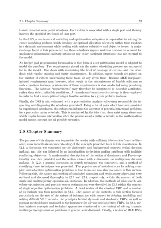

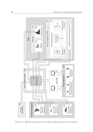
![3.1. Functional elements in an MLE environment 57
an MLE database and associated database manager. These functional elements, together with
the flow of information between them, are illustrated in Figure 3.1.
3.1.1 Overview of the proposed architecture
The first and most central functional element in Figure 3.1 is the MLE database manager and
its associated central database, denoted in the figure by (a) and (b), respectively. This database
is a storage and retrieval mechanism housing a large collection of data, and it also serves as
the communication hub of the system from where data are continually transmitted between
the functional elements of the system — all functional elements therefore communicate with one
another via this database. The associated database manager is responsible for managing updates
to or facilitating queries for MLE operations-related data as well as processing and converting
output data from one functional element to the correct input data format for another.
The HMI in Figure 3.1(c) is the link between man and machine; it enables a human operator to
communicate with the functional elements of the system by providing him with an interactive
graphic user interface which displays the situation at sea in real time together with the results
generated by the other functional elements on a series of computer screens. It is advocated that
this transfer of information should be implemented in the form of so-called data streams, which
are strings of bits associated with identifiers that allow an operator to request specific data in
real time. These streams may be fed live to the HMI and, depending on whether or not they
are activated by the operator, may be visualised on a display screen. For instance,
[VesselIdentifier; (Long,Lat); Course; Speed] = [0020; (−35.83, 18.90); 120.3; 18]
is an example of a snapshot from a data stream which may be visualised in a user-friendly
fashion via the HMI for the benefit of a threat detection operator, while
[VesselIdentifier; Status; FlagCode] = [0113; Flagged; ZoneInfraction]
is an example of a data stream snapshot which may be displayed similarly via the HMI for the
benefit of a threat evaluation operator. Here, the “VesselIdentifier” data field is used as a unique
identifier for attaching information to a particular VOI.
In this system architecture, it is proposed that, as the MLE threat detection and threat eval-
uation processes tend naturally to function closely together, so too should the MLE resource
assignment operators in Figure 3.1(d) work closely together with the MLE threat detection and
threat evaluation operators. In certain cases, however, where there are a very limited number of
MLE human resource operators, or if a certain human operator has considerable expertise in all
three MLE areas, one or a small number of operators may very well be responsible for decision
making in all aspects of MLE.
The external threat detection infrastructure functional elements in Figure 3.1(f) comprise all
devices used, directly or indirectly, for detecting and tracking maritime objects in specified areas
of the ocean as well as for gathering kinematic information associated with these objects, such as
their sizes, locations and velocities. Examples of such threat detection devices are land-based,
aerial or vessel-based radars, infrared cameras, video surveillance cameras and observations
reported from active naval, aerial or reconnaissance MLE resources.
These measured attributes of VOIs, obtained from the sensor systems, are fused together by
the attribute management system in Figure 3.1(e) to create so-called system tracks and derived
attributes associated with each of the VOIs within the jurisdiction area of the coastal nation [49].](https://image.slidesharecdn.com/6cd1ebf5-5cfe-4d40-998c-99cbe17b08f1-170109122537/85/PhD-dissertation-89-320.jpg)
![58 Chapter 3. System Architecture
A system track is a record of the historical displacement of a VOI in space from its detection
to the present time, while a derived attribute of a VOI is a parameter value that is computed
from the measured attributes of the VOI, such as its acceleration or rate of changing course.
Based on these attributes, the system also provides future VOI trajectory estimates to the DSSs.
Track stitching methods and Markov models are examples of techniques that may be employed
to assemble system tracks [49].
This fusion process is conducted by employing all data and knowledge associated with a VOI
and results in a combination of these elements into a single consistent, accurate, and useful data
representation for that VOI. Successfully implementing the fusion process is critical in cases
where VOI input data are obtained from multiple threat detection infrastructure sources which
may individually yield slightly or significantly different perspectives on information. The JDL
data fusion model, for example, is perhaps the most widely-used method for categorizing data
fusion-related functions [2]. This model has been shown to be useful across multiple application
areas and is typically intended to identify the processes, functions, categories of techniques, and
specific techniques applicable to data fusion.
In order to filter VOIs from the multitude of maritime objects tracked at sea within the jurisdic-
tion area of a coastal nation, threat detection operators are tasked with analysing these objects
in respect of the physical and kinematic information attached to them, and assessing whether
their behaviour is deemed unexplained, suspicious or threatening (to some extent). Following
this analysis, the status of a maritime object may be designated as either a VOI or a maritime
object of no interest. This procedure must be carried out on a continual basis as the situation
at sea unfolds, typically involves a large number of maritime objects and may therefore easily
overwhelm a human operator. The aim of the VOI flagging functional element in Figure 3.1(j)
is to assist human operators in their threat detection decisions by providing automated decision
support for identifying and tracking suspicious maritime activities.
An adaptive early-warning maritime surveillance DSS capable of supporting a maritime oper-
ator in his decision making process with regard to various threats and scenarios was proposed
by du Toit [49]. Here, so-called fusion, rule-based system, activity classifier and data mining
components are incorporated into the proposed DSS. Moreover, the HMI component in this DSS
provides the operator with relevant information as well as a mechanism by which the operator
may provide feedback to the system. The fusion component, for instance, processes the infor-
mation received from threat detection devices, such as radars or infrared cameras, in the form of
vessel track updates, which are stored in an operational database. This operational database is
directly utilised by the rule-based system component which processes the data as they become
available and aims to identify potentially threatening activities amongst the observed vessel
tracks according to certain pre-configured sets of rules, such as rules pertaining to zone infrac-
tions, proximity of vessels or anomalous activities. Data from the operational database are
migrated to a central database after being cleaned and transformed into the necessary format.
As tracks become available in the central database, they are processed by the activity classifier
component. The work in [49] is strictly limited to the maritime domain and the primary source
of data is spatio-temporal AIS data.
The input data provided by the external threat detection infrastructure functional elements may
not always provide all the information necessary to facilitate good inferences with respect to the
potentially threatening nature of a VOI. The external MLE threat evaluation infrastructure
functional elements in Figure 3.1(g) comprise a collection of physical devices which may be
used, when requested by an operator, to collect more detailed and/or accurate information
related to a particular VOI. Scouting resources (such as unmanned airplanes) dispatched to
specific maritime zones in order to establish line-of-sight contact with respect to targeted VOIs,](https://image.slidesharecdn.com/6cd1ebf5-5cfe-4d40-998c-99cbe17b08f1-170109122537/85/PhD-dissertation-90-320.jpg)
![3.1. Functional elements in an MLE environment 59
and advanced radar systems whose primary function is effectively to zoom in on particular VOI
locations, are examples of such devices.
The purpose of the VOI threat analysis DSS in Figure 3.1(i) is to assist a threat evaluation
operator in classifying and quantifying the potentially threatening nature of VOIs, by providing
automated decision support for analysing the behaviour of VOIs based on the information col-
lected during the threat detection process and making automated inferences with respect to the
nature and level of threat posed by VOIs. This process therefore only involves system tracks
of VOIs and not the tracks of maritime objects deemed of little or no interest. Ultimately, the
output of such a DSS consists of a vector associated with each VOI containing entries which
correspond to estimated probabilities with which the VOI in question belongs to a finite number
of pre-determined threat classes, an unknown threat class and a false alarm class. Various math-
ematical models may underlie this process of quantifying these probabilities. Bayes’ theorem
may, for example, be used as a framework for introducing newly observed information [9, 36].
The MLE resource assignment subsystem in Figure 3.1(l) is responsible for assisting human
operators with decisions related to the utilisation of MLE resources in both time and space.
These MLE resources are generally either allocated for the purpose of intercepting VOIs at sea
(such resources are said to be in an active state) or are otherwise strategically allocated to
certain patrol areas at sea or moved to bases until needed for future law enforcement purposes
(such resources are said to be in an idle state). Whereas the MLE response selection DSS
in Figure 3.1(m) deals with the allocation of active MLE resources, the idle MLE resources
management in DSS Figure 3.1(n) deals with the allocation of idle MLE resources. These two
functional elements should operate in perfect real-time synchronisation with one another.
Tasks performed within the idle MLE resources management DSS involve, inter alia, the config-
uration of patrol schedules, the planning of repair and maintenance of resources and the design
of effective scouting strategies. This DSS should combine the expertise and experience of human
operators with large amounts of historical data (e.g. probability distributions of specific threat-
ening activities occurring in specific zones of the jurisdiction area over specific time intervals)
and various mathematical models for scheduling idle MLE resources in both time and space.
Because occurrences of newly detected VOIs are stochastically distributed in space and time, it
is crucial to manage idle MLE resources in such a way that leaves them, a posteriori, in central
positions of relative readiness so that they may be dispatched rapidly when shifted into an active
state.
3.1.2 External MLE resource assignment infrastructure
As discussed earlier, all physical infrastructure elements dealing with the assignment of MLE
resources reside in the external MLE resource assignment infrastructure functional element class
in Figure 3.1(h). Five major components that are relevant to MLE response selection operations
have been identified. These are a geographical information system model of the jurisdiction area,
used to define clear boundaries at sea and to incorporate rules and regulations that are applicable
within these boundaries; a set of decision making entities comprising the various MLE resource
assignment role players of a coastal nation; an MLE fleet of resources comprising one or more
classes of units, each class possessing a clear, unique set of attributes and capabilities as well
as a parent decision entity; a set of MLE resource assignment bases providing various types of
essential services to idle MLE resources; and a set of pre-defined circuits used for patrol purposes.
These five components are described in more detail in this section.](https://image.slidesharecdn.com/6cd1ebf5-5cfe-4d40-998c-99cbe17b08f1-170109122537/85/PhD-dissertation-91-320.jpg)
![60 Chapter 3. System Architecture
The jurisdiction area
The set of the maritime zones, as defined in the UNCLOS [151], should be used as a guideline to
define the maritime law enforcement boundaries of a coastal nation. These boundaries should
therefore at the very least enclose the territorial seas, the contiguous zone and the exclusive
economic zone as jurisdiction areas, but these areas may be subdivided or refined further, as
required by the coastal nation in question in order to meet specific MLE goals. Farina et al.
[55], for example, simulate a maritime border control environment with an off-limit zone and
a warning zone, measured at 20 km and 50 km from the coastal baseline, respectively. The
jurisdiction area of a coastal nation may be modelled using shape-lines generated by standard
Geographic Information System software packages.
The decision entities
As mentioned in §1.2, it is typically the case that the entire MLE response selection process
of a coastal nation is not conducted by a centralised operator assisted by a single DSS, but
is rather orchestrated by multiple role players, called MLE decision entities. These decision
entities may perceive the quality of MLE response selection operations in their own, different
ways, as they each tend to pursue their own goals and subjective perceptions of what is deemed
important while carrying out MLE operations. In particular, these decision entities may perceive
the threatening intensity of VOIs differently, function largely independently from one another,
follow their own guidelines, and utilise their own subsets of MLE resources.
The South African Navy, the South African Maritime Safety Authority (SAMSA) and the De-
partment of Agriculture, Forestry and Fisheries (DAFF) are three examples of major decision
entities in the South African MLE environment [49]. While the South African Navy specialises
in investigating and neutralising acts of piracy, threats to sovereignty1 and terrorism threats,
SAMSA specialises in investigating and neutralising incidents of pollution, accidents at sea and
hazardous vessel threats, while DAFF resources specialise in investigating and neutralising illegal
fishing threats. Sometimes these decision entities function independently and sometimes they
collaborate. For example, the South African Navy and SAMSA often combine their resources
when investigating and neutralising smuggling and illegal immigration threats.
The MLE resources
MLE operations require law enforcement resources capable of neutralizing a variety of threats
at sea. These resources perform differently, depending on their physical characteristics (such
as size, maximum speed, manpower on board, weapon system infrastructure and other defense
mechanisms, autonomy at sea, and set-up time). Here, the speed of a resource influences its
ability to intercept VOIs effectively, while its weapon system infrastructure and other defense
mechanisms determine its effectiveness with respect to neutralising threats. The autonomy of a
resource refers to its ability to be self-sufficient at sea for an extended period of time while on a
mission, whilst its set-up time refers to the time required to prepare the resource for departure
on a mission.
The optimal resource fleet composition of MLE resources is not addressed as part of this MLE
resource assignment problem; the set of MLE resources at the disposal of a coastal nation is
normally assumed fixed and, consequently, the fixed costs associated with the acquisition of MLE
1
A foreign warship arriving unannounced in the jurisdiction area of a coastal nation constitutes a threat to
the sovereignty of the coastal nation.](https://image.slidesharecdn.com/6cd1ebf5-5cfe-4d40-998c-99cbe17b08f1-170109122537/85/PhD-dissertation-92-320.jpg)
![3.1. Functional elements in an MLE environment 61
resources are external to the problem. The variable (set-up and operating) costs associated with
these resources are, however, taken into consideration.
The simulator proposed by Farina et al. [55], for example, incorporates two types of resources,
namely a helicopter and a patrol boat. Here, the resource response time is calculated based on
the velocity of the target and the resource parameters. The system considers the current MLE
resources available in order to select an appropriate resource to be dispatched to intercept the
target. The resource parameters considered in [55] are availability, speed, inspection time and
departure time.
The MLE resource bases
A base may be defined as a facility providing the necessary re-supplying, stationing and main-
tenance services to MLE resources. Every base is typically unique with respect to certain
characteristics that are relevant to resource assignment operations, such as size, accessibility
or geographical location. These characteristics, combined with external factors, may have a
significant impact on the way MLE resource assignment operations are conducted. Bases may
be classified as either inland, coastal or deployable. Inland bases are usually accessible to only
certain types of MLE resources if connected to the maritime jurisdiction area via a network of
rivers, or only accessible to aerial MLE resources otherwise. Coastal bases are located at fixed
locations along a coastline and provide a vast range of services to a variety of MLE resource
types. Finally, deployable bases have the ability to be dispatched in both time and space, from
where they, themselves, may dispatch fixed sets of MLE resources associated with the particular
bases.
The work of Malik et al. [91], for example, deals with the optimal allocation of MLE resources
distributed amongst three stations (bases) to undertake assignments in the Great Lakes region
of North America. The study focused on determining the spatial and temporal distribution of
response cases and their assorted MLE resources for all search and rescue operations and how
closing any one of these three stations may affect the workload of the other stations that would
subsequently be required to absorb the additional tasks. It was concluded that the closure of
auxiliary stations would imply longer response times, which may potentially translate into the
loss of lives and property. Overall, the DSS in place allowed users to conduct a sensitivity
analysis by determining the change in risks associated with closing certain stations in terms of
the success rate of search and rescue operations in the medium and long run.
The patrol circuits
In an MLE environment, the notion of patrol may be described as the strategic allocation of
idle MLE resources in specific regions of the jurisdiction area. A patrol circuit may be any pre-
defined maritime zone boundary, route or singular point to which an idle MLE resources may
be assigned strategically. A patrolling MLE resource typically breaks away from its designated
patrol circuit as a result of one of the following occurrences: (a) the MLE resource has travelled
further than a certain maximum distance threshold and is re-allocated to performing a different
task, (b) the MLE resource has travelled for more than a pre-determined maximum amount of
time since it was last re-supplied and is therefore re-allocated to performing a different task, (c)
the MLE resource is assigned a mission to intercept one or more VOIs (i.e. the MLE resource
transits from an idle state to an active state) or (d) an operator decides to re-allocate the MLE
resource to a different patrol circuit or to a base for any reasons other than the occurrences (a)
and (b) above.](https://image.slidesharecdn.com/6cd1ebf5-5cfe-4d40-998c-99cbe17b08f1-170109122537/85/PhD-dissertation-93-320.jpg)
![62 Chapter 3. System Architecture
Shieh et al. [129], for example, introduce an interesting game theoretic DSS premised on an
attacker-defender Stackelberg game model, where the adversary is defined as an individual with
ties to al-Qa’ida. This DSS has been deployed by the US Coast Guard to schedule patrols
around the port of Boston. The DSS is currently in the process of being deployed around the
port of New York as well.
3.1.3 The MLE response selection DSS
The proposed core MLE response selection DSS consists of a model generation subsystem, a
model solution subsystem and an information management subsystem. The model genera-
tion subsystem comprises a model configuration component, which allows for the construction
and storage of fundamental mathematical structures and modelling components (such as ob-
jective functions, routing constraints and MLE resource parameters), and a model management
component, which accommodates dynamic features that are used to model the problem on a
temporal basis. The solution search subsystem is concerned with finding and presenting a set
of non-dominated trade-off solutions to the MLE response selection operator for every prob-
lem instance formulated in the mathematical modelling subsystem. The first component of the
information management subsystem is the problem instance reinitialisation component, which
is responsible for detecting significant changes in input data transferred from relevant external
sources, and to inform the operator of the extent and nature of these changes. The second
component is the optimisation tracker component, which acts as an independent, automated
solution search engine; its purpose is to track the (possibly approximate) Pareto-optimal set of
solutions in real time while considering all input data changes taking place. The last component
is the solution tracker component. Here, solution tracking may be thought of as an independent
process which continuously updates, filters and stores strategic solutions to the current real-time
situation for eventual use in MLE response selection-related decisions. This component is also
responsible for communicating minor changes observed in the currently implemented solution
to micro-management role players, following which the necessary adjustments in solution imple-
mentation can be made. These subsystems share input data via the centralised MLE database,
as illustrated schematically in Figure 3.2. Here, the external data sources node refers to input
data received from functional elements that are external to this DSS (see Figure 3.1).
The overall working of the proposed MLE response selection process is summarised as follows.
A new cycle of the DSS, or problem instance, is initiated whenever the problem instance reini-
tialisation component detects a significant change in input data. This event in time is called a
disturbance. Disturbances may cause the currently implemented solution no longer to be con-
sidered the most preferred MLE response selection alternative, as these are typically likely to
cause current solution changes on a macroscopic level. The rate of reinitialisation of problem
instances over time is therefore proportional to the rate of flow of events triggering disturbances.
Before the next problem instance may be initiated, however, it is advocated that the operator
be required to confirm that the detected changes in input data are indeed categorised as a
disturbance.
Following the advent of a disturbance, the new MLE situation is remodelled as a new MLE
response selection problem instance in the model configuration component. In addition, the
operator should be able to participate in the process by contributing input based on his expertise
in the field in respect of certain subjective conditions or preferences related to the current MLE
situation via the model management component.
Following the mathematical modelling process pertaining to a problem instance, the solution
search subsystem is required to find a high-quality, filtered set of so-called non-dominated solu-](https://image.slidesharecdn.com/6cd1ebf5-5cfe-4d40-998c-99cbe17b08f1-170109122537/85/PhD-dissertation-94-320.jpg)
![3.2. The chronological order of MLE events 63
Mathematical Modelling Model Solution
Model configuration
Model management
Optimisation methodology
Post-optimisation
solution analysis
MLE Database
External
Data Sources
Information management
Optimisation
tracker
Problem instance
reinitialisation
Solution
tracker
Figure 3.2: The MLE response selection DSS with its three subsystems and their components.
tions in multiobjective space using effective (metaheuristic) search techniques. Because the time
elapsed between the previously implemented solution and the new one causes a deterioration in
the effectiveness of MLE response selection operations, it is critical for these search techniques
to be able to find high-quality solutions to the new problem instance in a very limited time.
The operator is then required to select a single (most preferred) alternative from this set of
suggested trade-off solutions in the post-optimisation solution analysis component, which con-
sists in assigning a subset of MLE resources to intercept and investigate a subset of VOIs. This
solution should finally be communicated to the MLE database, from where the various MLE
response selection decision entities and other various role-players may immediately be notified
of the changes in routing implementations brought along by this new solution.
Meanwhile, the optimisation tracker and solution tracker components should operate in parallel
along a time continuum, tracking a high-quality, highly diverse set of non-dominates alterna-
tives and managing these alternatives as the MLE response selection situation changes in real
time and new input data are made available. These solutions should be made available to the
mathematical modelling and model solution subsystems at the start of a problem instance as a
means of speeding up the decision making process brought along by the start of a new problem
instance.
3.2 The chronological order of MLE events
The functional elements described in the previous section operate as part of a so-called MLE
cycle of events, inspired by the so-called Threat Evaluation Weapon Assignment cycle proposed
by L¨otter & van Vuuren [89] in the context of ground-based air defense. A trigger of such a
cycle initiates consecutive calls to these elements in an orderly fashion so as to provide updated
data to the operators in real time. It is assumed that an MLE cycle is triggered by a significant
change in any of the input data fields of the MLE database or by the natural continuation of an
implementation clock cycle. The sequential order in which the functional elements are utilised
within an MLE cycle is illustrated graphically in Figure 3.3.](https://image.slidesharecdn.com/6cd1ebf5-5cfe-4d40-998c-99cbe17b08f1-170109122537/85/PhD-dissertation-95-320.jpg)
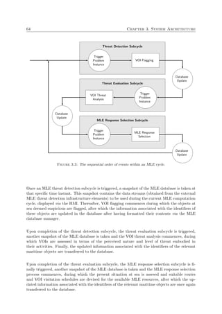
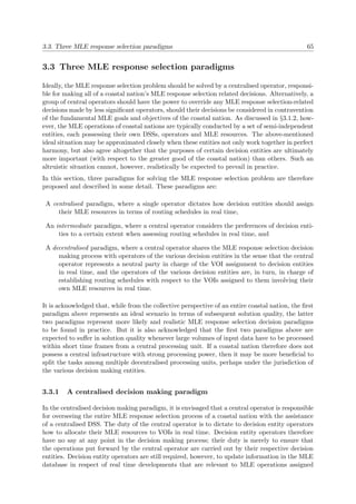
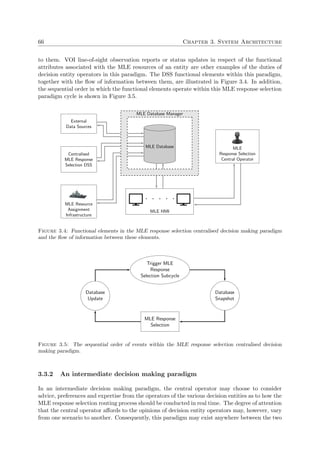
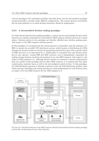
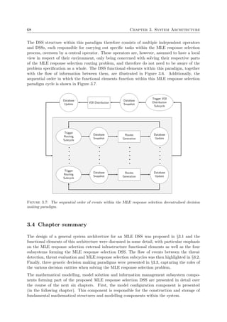
![4.1. Concepts and assumptions 71
There are two main reasons for suggesting the specification of decision entity preferences in such
a format, rather than requesting ideal subsets of VOIs preferred by each of the decision entities.
First, some of the VOIs in such ideal subsets may be more important to the respective decision
entity than the other VOIs in those subsets, and the VOI distribution process should account
for such relative importance measures. Secondly, it may be the case that VOIs outside the ideal
subset expressed by a decision entity are allocated to it, and because this decision entity also
has certain preferential levels with respect to those VOIs, the VOI distribution process must
also account for this possibility.
4.1.2 Vehicle routing characteristics
In this dissertation, it is proposed that instances of the MLE response selection problem be
modelled as a special type of VRP, described in detail in §2.6. In the MLE response selection
VRP, the depots represent the bases from whence MLE resources are dispatched, the fleet of
vehicles represents the fleet of MLE resources at the collective disposal of the decision entities
and the customers represent the VOIs tracked at sea within the territorial waters of the coastal
nation. The process of investigating and possibly neutralising VOIs is analogous to visiting and
servicing a customer in the context of a traditional VRP application. Moreover, the notion of
patrol circuits in an MLE response selection environment, described in §3.1.2, serves a similar
purpose to the repositioning-and-waiting strategies in anticipation of future events in the VRP
literature [150]. Here, idle vehicles currently situated in low-demand areas are relocated to cover
high-demand areas (preferably not too far from a base, depending on the autonomy levels of
these vehicles), also known as “areas of interest” or “fruitful regions,” based on known a priori
information in the form of historical data related to previous events.
The MLE response selection problem differs from standard capacitated VRP formulations in the
literature as a result of the following characteristics:
1. The fleet of vehicles is not necessarily homogeneous,
2. servicing a customer is optional,
3. assigning a vehicle a route is optional,
4. certain types of vehicles are not suitable to visit certain types of customers,
5. certain types of vehicles are favoured to visit certain types of customers,
6. vehicles are typically not subject to capacity restrictions in the classical sense,
7. the number of customers is not fixed and neither are their locations,
8. the distance between any two customers is not necessarily the same in both directions,
9. the length of a travel arc between any two customers is measured as the shortest possible
path linking them aquatically (except in the case of aerial MLE resources),
10. certain situations may require that more than one vehicle be assigned to visit a customer,
11. there may be more than one (inhomogeneous) depot,
12. a vehicle may start out along a route that does not originate or end at a depot,
13. idle vehicles do not have to be stationed at a depot,](https://image.slidesharecdn.com/6cd1ebf5-5cfe-4d40-998c-99cbe17b08f1-170109122537/85/PhD-dissertation-103-320.jpg)
![72 Chapter 4. Model Configuration
14. a vehicle route may start at a certain depot and end at a different one, and
15. certain depots may not necessarily have fixed locations.
In the above list, Characteristics 1–3 follow from the discussion in §2.6 on certain variants of
the VRP in the literature. VRPs of the kind mentioned in Characteristic 1 are known in the
literature as VRPs with a Heterogeneous Fleet [150], while VRPs of the kind mentioned in
Characteristic 2 are known in the literature as VRPs with Customer Profits [1].
Characteristic 4 places the restriction that certain types of MLE resources should preferably not
be scheduled to intercept VOIs that are suspected to be of a certain type, as their infrastruc-
ture characteristics may not be effective enough to successfully neutralise threats of that type.
Similarly, taking into account the unique properties that are regarded to be advantageous in
successfully neutralising threats of certain types, Characteristic 5 encourages certain kinds of
MLE resources to preferably intercept VOIs that are suspected to be threats of these types.
Characteristic 6 stresses that the MLE resources are typically not restricted to a capacity con-
straint (in terms of delivering commodities to customers, as is the case in most VRP problem
formulations in the literature), but are rather constrained in terms of maximum distances trav-
elled or lengths of time associated with the routes of the vehicles as a result of various practi-
calities, such as the need to refuel or resupply materials or ammunition, the need to perform
routine MLE resource maintenance and the need to allocate leave or periods of rest to crew
members. VRPs of this kind are known in the literature as Distance-Constrained VRPs and
Time-Constrained VRPs [150].
Characteristic 7 acknowledges the kinematic nature of VOIs at sea, calling for interception
points to be calculated, while Characteristic 8 allows for the possibility that MLE resource
travel directions are influenced by ocean currents and adverse meteorological conditions. VRPs
of this kind are known in the literature as Asymmetric VRPs [150]. Characteristic 9 refers to the
open spherical nature of an oceanic jurisdiction area (barring navigation movement constraints
such as land masses, shallows, weather and EEZ boundaries), while Characteristic 10 refers to
types of VOIs that do not only involve high threatening intensities, but where it is also deemed
necessary to allocate multiple MLE resources to them in order to successfully neutralise them.
VRPs of this kind are known in the literature as VRPs with Split Deliveries.
Characteristic 11 is applicable to coastal nations having more than one base from whence MLE
resources are dispatched. VRPs of this kind are known in the literature as Multi-Depot VRPs
[150]. In such a case, Characteristic 12 focuses attention on the fact that an MLE resource may
be diverted to a new route while out at sea or to a patrol circuit (i.e. it is not required that
an MLE resource should first return to the base prior to starting out along a new route), and
Characteristic 13 allows for the resources to be on stand-by at sea in strategic locations until
assigned to a specific interception route. Finally, Characteristic 14 states that certain MLE
resources may start out from certain bases and return to other bases, while Characteristic 15
refers to coastal nations possessing certain types of mobile bases which may be deployed at sea
to provide basic services to certain subsets of MLE resources.
4.1.3 The objectives informing MLE response selection decisions
As hinted previously, it is proposed that the MLE response selection problem should be modelled
as a multiobjective VRP. Coastal nations (and their various decision entities) typically have their
own values, preferences and perceptions of the desirability of trade-offs between objectives when
dealing with threats at sea. It is therefore expected that the MLE response selections of the](https://image.slidesharecdn.com/6cd1ebf5-5cfe-4d40-998c-99cbe17b08f1-170109122537/85/PhD-dissertation-104-320.jpg)
![74 Chapter 4. Model Configuration
In order to accommodate the dynamic nature of the MLE response selection problem, a distur-
bance is defined as a threshold phenomenon occurring stochastically in time which may cause
the currently implemented solution to suffer in terms of quality and/or feasibility, hence trigger-
ing the start of a new problem instance during which the current situation is re-evaluated (i.e.
the instance is re-solved under the original information combined with the data update which
brought along the disturbance, disregarding those VOIs of the previous solution that have al-
ready been intercepted). Henceforth, define the notion of a time stage as a finite temporal
interval that marks the start and finish of a problem instance. A disturbance therefore causes
the current time stage to end and the next one to begin.
4.1.6 MLE resources counter-threat performances
As a result of their unique infrastructure, size, crew expertise and speed, certain types of MLE
resources excel at countering VOIs embodying certain types of threats. This is particularly the
case if a VOI embodies a type of threat for which the decision entity in charge of the MLE
resource scheduled to intercept this VOI specialises in countering threats of that type. Ensuring
that the right MLE resources are dispatched to intercept VOIs is beneficial for many reasons.
For instance, the ability to counter certain threats effectively keeps the danger of retaliations,
material damage and possible human injuries to a minimum. Furthermore, effectively investigat-
ing and/or neutralising VOIs reduces the service time. This is a crucial factor to accommodate
whenever the MLE resource has one or more VOIs to investigate on its visitation route after
having intercepted the current customer1.
It may be the case that a certain type of MLE resource does not only have a low efficiency
value in respect of countering certain types of threats, but also does not have the capacity to
successfully neutralise VOIs embodying certain types of threats. An MLE resource is defined to
be strictly incapable of neutralising a certain VOI if it is forbidden to attempt to neutralise a
VOI or incapable of neutralising a VOI embodying a (known) specific type of threat. Situations
in which MLE resources are assigned to VOIs that they are strictly incapable of neutralising
are defined as infeasible encounters2. Infeasible encounters would never occur if the threat
associated with any VOI were known in advance (assuming that the MLE response selection
routing operator is competent). As discussed in §4.1.4, however, expectations with respect to
the nature of VOIs are subject to error and, although the nature of certain VOIs are easily
detected and evaluated in respect of the threat that they embody, others may carry a high level
of uncertainty, in turn increasing the risk of infeasible encounters. The degradation in MLE
response selection operations caused by infeasible encounters may be measured by a penalty
function.
4.1.7 MLE resources autonomy levels
As stated in Characteristic 6 of §4.1.2, it is suggested that the MLE response selection problem
is, inter alia, formulated as a distance and time constrained VRP. Define the autonomy level of
an MLE resource with respect to distance, called its distance autonomy level, as the maximum
distance that it may travel at sea before having to return to a designated base. Similarly, define
the autonomy level of an MLE resource with respect to time, called its time autonomy level, as
the maximum time that it may spend at sea before having to return to a designated base.
1
The VOIs tracked at any time should generally be dealt with as quickly as possible to lower the chances of
their escape from the territorial waters of the coastal nation or losing their tracks on the radar.
2
Infeasible encounters are analogous to so-called service failures in the VRP literature [150].](https://image.slidesharecdn.com/6cd1ebf5-5cfe-4d40-998c-99cbe17b08f1-170109122537/85/PhD-dissertation-106-320.jpg)
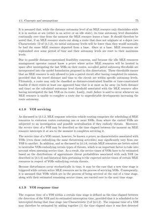
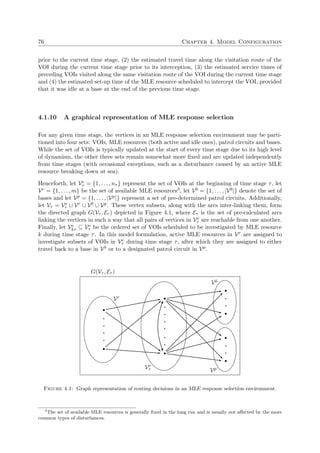
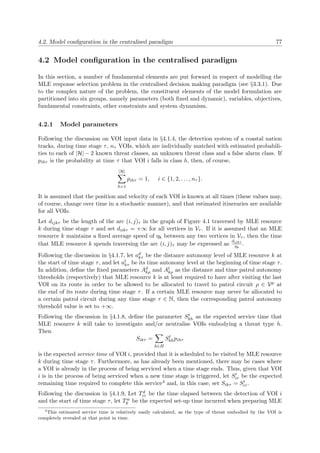
![78 Chapter 4. Model Configuration
resource k for a mission, and define the parameter
γkτ =
1, if MLE resource k is not on stand-by at the end of time stage τ − 1
0, otherwise.
Furthermore, let Tt
ikτ denote the expected transit times accumulated by MLE resource k along
its visitation route from the start of time stage τ until it reaches VOI i. Similarly, let Ts
ikτ denote
the expected VOI service times accumulated by MLE resource k along its visitation route from
the start of time stage τ until it services VOI i. Then
tiτ = Td
iτ + Tt
ikτ + Ts
ikτ + γkτ Tw
k
is the expected response time of VOI i during time stage τ, where
Tt
ikτ =
d0kτ ikτ
ηk
, if i = Ve
kτ (1)
d0kτ Ve
kτ
(1)kτ +
|Ve
kτ (i)|
j=2 dVe
kτ
(j−1)Ve
kτ
(j)kτ
ηk
, otherwise,
and
Ts
ikτ =
0, if i = Ve
kτ (1)
|Ve
kτ (i)|
=2 SVe
kτ ( −1)kτ , otherwise.
Here, the notation Ve
kτ (i) represents the ith VOI on the route of MLE resource k during time
stage τ while |Ve
kτ (i)| is a cardinal number representing the ordered position of that VOI on the
route. For example, if Ve
kτ = {5, 16, 9}, then Ve
kτ (3) = 9 and |Ve
kτ (9)| = 3. Furthermore, 0kτ
represents the initial position of MLE resource k at the beginning of the time stage. Finally, set
tiτ = 0 if VOI i was in the process of being serviced by a MLE resource when time stage τ − 1
ended. Of course, tiτ is set to 0 if it is not scheduled as part of any visitation route.
Next, the monetary cost associated with MLE resource k traversing the arc (i, j)τ in the graph
of Figure 4.1 during time stage τ is assumed to be estimated as Γkdijkτ , where Γk is the cost
per unit distance travelled associated with MLE resource k. Note that Γkdiikτ = +∞ holds for
all vertices in Vτ . In addition, define the set-up cost Cs
k incurred when preparing MLE resource
k for departure on a mission. Moreover, costs may be associated with trajectory deviations
from one route to another due to factors such as operational manoeuvres or disruption of the
original solution due to a disturbance. Hence, define the disruption cost Cd
k to be incurred if
MLE resource k was active at the end of time stage τ − 1 and was subsequently scheduled to a
new trajectory (i.e. sent on a different route) at the beginning of time stage τ (noting that such
a cost should not be fixed, but rather expressed as a function of the intensity of the disruption
for that particular situation). In relation to this last cost, let Jk(τ−1) ∈ Ve
τ be the next VOI that
was scheduled to be intercepted by MLE resource k at the end of time stage τ − 1 (provided
that the MLE resource was active then), or set Jk(τ−1) equal to the dummy value 0 otherwise
(noting that 0 /∈ Ve
τ for all τ ∈ N).
Following the discussion in §4.1.6 and Characteristics 4 and 5 of §4.1.2, it is furthermore necessary
to establish parametric values for the counter-threat performance of MLE resources. In this
respect, let Wkh ∈ [0, 1] be the score associated with the efficiency of MLE resource k in terms of
neutralising a class h threat. In addition, the nature and frequency of maritime threats detected
vary in different regions of the world, and different coastal nations typically face different types
of threats at different levels of harm or intensity. Thus, let the score Qh ∈ [0, 1] associated with
class h threats represent the priority level assigned by the coastal nation to neutralise threats](https://image.slidesharecdn.com/6cd1ebf5-5cfe-4d40-998c-99cbe17b08f1-170109122537/85/PhD-dissertation-110-320.jpg)
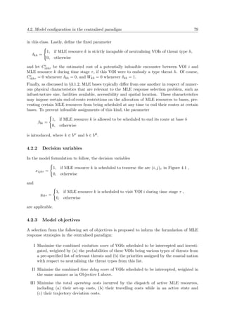
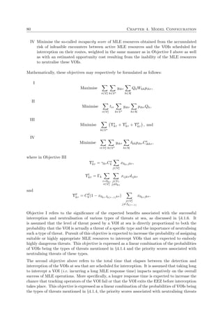
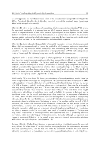
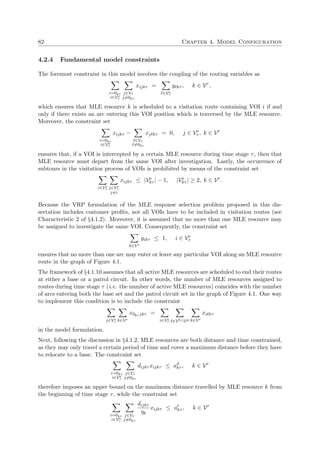
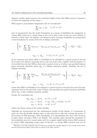
![84 Chapter 4. Model Configuration
allowed to operate inside certain maritime zones. Of course, this also includes the naive case
of attempting to service a VOI with a calculated intercept located on land. The mathematical
model of a given problem instance is therefore also expected to exclude solutions in which at
least one such infeasible interception point exists from the feasible decision space.
4.3 Model configuration in an intermediate paradigm
In this section, a number of constituent elements are put forward for modelling an MLE response
selection problem in an intermediate decision making paradigm (see §3.3.2). Because most of
the elements in this paradigm overlap with the ones presented for the centralised paradigm,
however, only previously unmentioned model elements are discussed in this section.
In addition to Objectives I–IV of the previous section, the following objective is proposed to
inform the formulation of MLE response strategies in an intermediate decision making paradigm:
V Maximise the combined consensus score obtained by aggregating the level of agreement of
each decision entity in respect of the set of VOIs assigned to it for MLE response selection
operations, weighted by (a) an individual VOI preferential ordered set associated with each
decision entity, (b) the deviation from the ideal quantity of VOIs assigned to each decision
entity and (c) the relative importance of each decision entity to the coastal nation.
Following the discussion in §4.1.1, this fifth objective deals with measuring the consensus level
achieved as a result of the assignment of VOIs to the various decision entities. It is assumed
that this consensus level is measured by the weighted sum of the deviation from the decision
entities’ ideal or preferred subsets of VOIs to those in the solution. These ideal subsets may be
constructed by selecting a certain number of elements from the preferential ordered set of VOIs
of each decision entity. This objective may be expressed in two parts. First, a linear combination
of the weighted scores of the level of VOI preference of decision entities and the VOIs distributed
to them may be calculated. Then, a linear combination of penalties may be derived based on the
deviation of the VOIs assigned to the decision entities from the ideal number of VOIs requested
by these entities.
It is suggested that the penalties be assessed as a certain fixed discrete function of the deviations
for three main reasons. First, a fixed function is necessary, in contrast to decision entity-based
subjective functions, so as to ensure that the level of consensus is measured neutrally with respect
to this objective, as there already exists a preferential weight associated with each decision entity
(i.e. some entities may be deemed more important than others with respect to achieving the
MLE goals of the coastal nation). Secondly, this function may be configured so as to reflect
the relative importance of distributing VOIs with respect to the preferential ordered sets of the
various decision entities to that of the deviation from the respective ideal subset sizes. Finally,
such a function allows for asymmetry where, for example, assigning more VOIs to a decision
entity than its ideal number is not penalised as strictly as assigning fewer VOIs.
Recall that Ve
τ = {1, . . . , nτ } is the set of VOIs observed at the beginning of time stage τ ∈ N,
and let Z represent the set of decision entities of the coastal nation. Let Zs ∈ [0, 1] be a weight
representing the relative importance of decision entity s ∈ Z to the coastal nation and define the
ordered set Osτ = {os1, . . . , osnτ } as the input data received from decision entity s with respect to
VOI distribution preferences, so that VOIs are ranked from most preferred (i.e. most desirable to
investigate) to least preferred, at the beginning of time stage τ. Also, define Nsτ ∈ {0, 1, . . . , nτ }
as the ideal number of VOIs that decision entity s would prefer to investigate during time stage](https://image.slidesharecdn.com/6cd1ebf5-5cfe-4d40-998c-99cbe17b08f1-170109122537/85/PhD-dissertation-116-320.jpg)
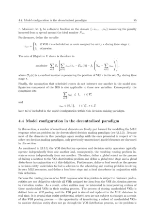
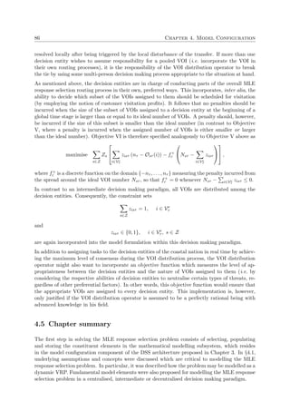


![CHAPTER 5
Model Management
Contents
5.1 The model management sub-components . . . . . . . . . . . . . . . . . . . . . . 90
5.2 The cutting plane sub-component . . . . . . . . . . . . . . . . . . . . . . . . . . 91
5.2.1 Exclusion sets for forbidden VOI assignments . . . . . . . . . . . . . . . 91
5.2.2 Inclusion sets for imposed VOI assignments . . . . . . . . . . . . . . . . 92
5.2.3 End-of-route assignments . . . . . . . . . . . . . . . . . . . . . . . . . . 94
5.2.4 Customer profit thresholds . . . . . . . . . . . . . . . . . . . . . . . . . 97
5.2.5 VOI distribution . . . . . . . . . . . . . . . . . . . . . . . . . . . . . . . 97
5.3 The model adaptation sub-component . . . . . . . . . . . . . . . . . . . . . . . 98
5.3.1 Combined assignments . . . . . . . . . . . . . . . . . . . . . . . . . . . . 98
5.3.2 Non-operational MLE resources . . . . . . . . . . . . . . . . . . . . . . . 100
5.3.3 Capacity restrictions . . . . . . . . . . . . . . . . . . . . . . . . . . . . . 101
5.3.4 Deployable bases . . . . . . . . . . . . . . . . . . . . . . . . . . . . . . . 101
5.4 Comments . . . . . . . . . . . . . . . . . . . . . . . . . . . . . . . . . . . . . . . 102
5.5 Chapter summary . . . . . . . . . . . . . . . . . . . . . . . . . . . . . . . . . . 102
In common with many routing and scheduling applications, the amount of informa-
tion needed to define the problem is large. This information is more than just a list of
rules and regulations and consists of both documented and undocumented knowledge,
subject to both soft and hard interpretation which may be objective or subjective. It
would appear at first sight that routing and scheduling is highly structured and well
defined but the problem in practice is usually less clearcut. — R. Fink [38]
In an MLE response selection environment, it may be very difficult to satisfy all constraints
and meet all goals when developing a set of routes, either manually or automatically, based
on mathematical programming. A number of important features demonstrating the dynamism
of the mathematical modelling process of the MLE response selection problem are presented
in this chapter as a way of improving model flexibility to adapt to certain situations. More
specifically, following a disturbance, or simply from a subjective preferential point of view, MLE
operators may wish to provide additional input information to a problem instance in order to
accommodate a variety of special requests into the model prior to launching the solution search
process for the next time stage. The model management component provides operators with a
89](https://image.slidesharecdn.com/6cd1ebf5-5cfe-4d40-998c-99cbe17b08f1-170109122537/85/PhD-dissertation-121-320.jpg)
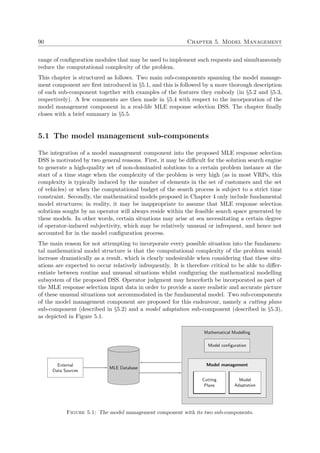
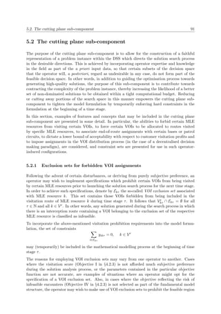
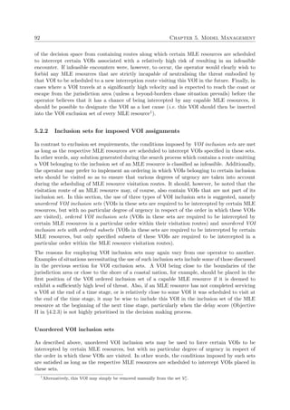
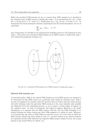
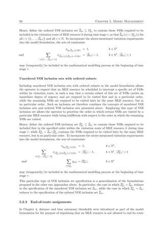
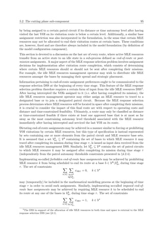
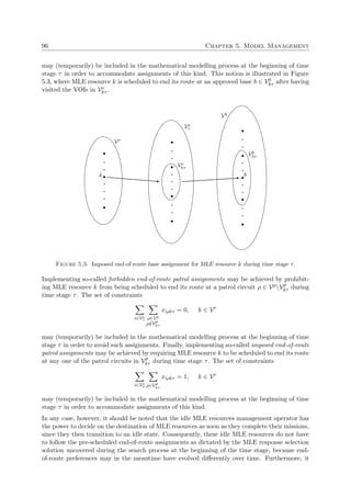
![5.2. The cutting plane sub-component 97
is critical for both resource assignment DSSs to work together when configuring these end-of-
route assignments; if the idle MLE resources manager is too strict with respect to end-of-route
destination decisions, it may prevent very good routes from being scheduled, as certain active
MLE resources may be restricted to travel within unnecessarily constrained zones. Hence, it is
the duty of the idle MLE resource manager to ensure that MLE response selection operations
do not suffer significantly as a result of poorly configured end-of-route assignment input data.
5.2.4 Customer profit thresholds
As was mentioned in Characteristic 2 of §4.1.2, any subset of VOIs may be serviced during any
time stage. The search process is therefore configured to explore a possibly large variety of
subsets in solution space in order to generate an acceptable spread of non-dominated solutions.
The operator may, however, be inclined to focus his preferences on solutions with high visitation
scores a priori (see Objective I in §4.2.3). Because a good upper bound on the visitation score
is known in advance, however, it may be impractical to reduce the search space according to a
pre-determined numerical score in this respect. Since the number of VOIs visited in a solution
positively correlates to its visitation score, and because the number of VOIs at the beginning of
a time stage is known, the operator may nevertheless be able to specify a threshold in the form
of a minimum proportion of all VOIs that should be intercepted during the current time stage3.
Such a threshold should ensure that the search process does not waste resources investigating
solutions in which the subset of intercepted VOIs is deemed too small.
Hence, define a so-called customer profits threshold parameter ∆τ ∈ [0, 1] as the minimum
proportion of VOIs that have to be intercepted during time stage τ; i.e. solutions that do not
satisfy the inequality
k∈Vr
Ve
kτ ≥ nτ ∆τ
are classified as infeasible. In order to implement this requirement, the set of constraints
i∈Ve
τ k∈Vr
yikτ ≥ nτ ∆τ
may (temporarily) be included in the mathematical modelling process at the beginning of time
stage τ.
5.2.5 VOI distribution
Only model management features for use in the MLE response selection routing process have
been proposed up to this point. Additionally, the VOI distribution model presented in §4.4 may
also be subject to dynamic elements, as requested by the VOI distribution operator (provided
that he has the power to do so). In particular, he may decide a priori to assign one or more
specific VOIs to certain decision entities4.
Hence, define the VOI distribution inclusion set Is
τ to contain those VOIs required to be allocated
to decision entity s during time stage τ, noting that Is
τ ⊆ Ve
τ for all τ ∈ N and all s ∈ Z. In
3
If the operator most often exhibits the same preferences, then these conditions may be incorporated as part
of the model configuration component.
4
The notion of prohibiting certain VOIs from being assigned to certain decision entities appears to be unrealistic
and is thus omitted from the discussion.](https://image.slidesharecdn.com/6cd1ebf5-5cfe-4d40-998c-99cbe17b08f1-170109122537/85/PhD-dissertation-129-320.jpg)
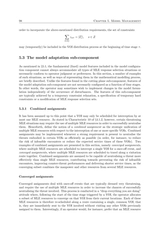
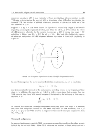
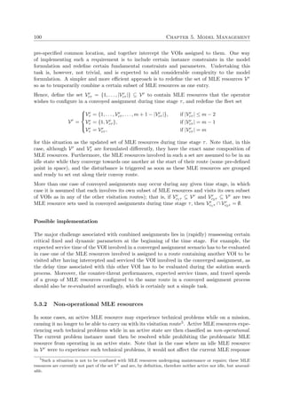


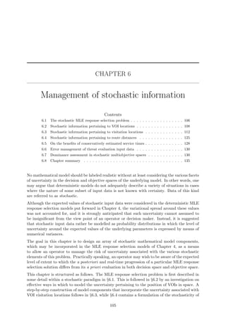
![106 Chapter 6. Management of stochastic information
route travel distances. In §6.5, a brief discussion on the uncertainty pertaining to VOI service
times is conducted, after which the management of uncertainty pertaining to the threatening
nature of VOIs is addressed in §6.6. The focus then shifts in §6.7 from the impact that stochastic
elements have on the feasible decision space to the impact they have on the evaluation of solution
performances in objective space. The chapter finally closes with a brief summary in §6.8.
6.1 The stochastic MLE response selection problem
All models are wrong, but some models are useful. — G. Box [11]
Although the mathematical models derived in Chapter 4 may seem potentially useful, it is
foreseen that the progression of the visitation routes over the course of a given time stage is very
unlikely to turn out almost exactly as planned a priori. In fact, it is critical to acknowledge,
for the sake of realism, that the level of unpredictability in the development of visitation routes
in most real-life scenarios may even be so high as to not give the MLE response selection DSS
presented in this dissertation any edge over human operators in addition to validating their
decisions.
For this reason, it is both advocated and stressed that the level of practicality and realism in the
a priori configuration of MLE response selection solutions will most often only be as strong as
the levels of uncertainty enveloping its stochastic constituents. In particular, it is important to
concede that the modelling and optimisation techniques designed for incorporation in the DSS
will only be useful and effective if the quality of information is able to meet a certain standard.
Realistically speaking, the aim of this DSS should therefore rather be redefined as follows: To
provide an MLE response selection operator with real-time guidance on the macro-assignment of
MLE resources with respect to the seemingly best course of action to be taken given the nature,
quantity and quality of relevant information available at present.
6.1.1 General sources of uncertainty
In order to better understand the inherent stochastic nature of the MLE response selection
problem, it is first necessary to discuss the general sources of uncertainty that the MLE response
selection DSS must accommodate. Three such sources particularly stand out. As is often the case
with dynamic semi-automated DSSs in general, the first and most important uncertainty factor
in the configuration and implementation of desired routing solutions deals with the quantity,
format, accuracy and timeliness of input information received from the external data sources.
As mentioned earlier, the performance of an MLE response selection DSS will only be as good
as the standard of information provided to it, and so the general level of performance of external
systems of a given coastal nation will therefore ultimately determine whether such a DSS is
worth implementing.
The second source of uncertainty has to do with human error, in which various role players (such
as decentralised operators or MLE resource operators) fail to implement the solution proposed
by the DSS and MLE response selection operator in the recommended manner. A differentiation
is, however, made between situations in which a human role player presumably unintentionally
operates in ways that lead to a deterioration of the currently implemented solution, and in
which a human role player deliberately takes actions in real time in order to adjust operations
in certain ways so as to best conform to the current solution being implemented. Rational,](https://image.slidesharecdn.com/6cd1ebf5-5cfe-4d40-998c-99cbe17b08f1-170109122537/85/PhD-dissertation-138-320.jpg)
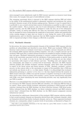
![108 Chapter 6. Management of stochastic information
In this diagram, a node succeeded by one or more other nodes indicates that its underlying
parameter estimators are (partially) derived from these preceding sources. In the remaining of
this chapter, the MLE response selection stochastic elements are considered and analysed in
greater detail.
Database
Snapshot
VOI
Location
VOI
Velocity
VOI
Intercept
VOI
Threat
Visitation
Score
VOI
Service
Time
Arc Travel
Distance
Arc Travel
Time
Delay
Score
Travel
Costs
Route
Feasibility
Status
Database
Update
Database
Update
Database
Update
Figure 6.1: Stochastic elements of the MLE response selection problem and the inter-computational
connections between them.
6.2 Stochastic information pertaining to VOI locations
Tracking and predicting the positions of VOIs in real time is probably the most crucial stochastic
feature of the MLE response selection problem, particularly because it provides the basis from
which most other MLE response selection stochastic elements are derived (see Figure 6.1). In
this section, an effective manner in which to model the uncertainty pertaining to the positions
of VOIs in space is pursued, after which the impact of threat detection systems performance on
the tracking of VOI locations is discussed.
6.2.1 The bivariate Gaussian probability distribution
In the remainder of this chapter, and with limited loss of generality, it is assumed that threat
detection systems are able to communicate the anticipated locations of VOIs in real time by
employing the bivariate Gaussian probability distribution [163] — a very popular case of elliptical
probability distributions for use in estimating the locations of objects in planar spaces [132, 137].
If the coordinates (Xi, Yi) represent random variables modelling the position of VOI i along the
axes of some two-dimensional global frame of reference, then (Xi, Yi) ∼ N(µiX, µiY , σ2
iX, σ2
iY , ρi)
with joint probability density function
fN (xi, yi) =
exp − 1
2(1−ρ2
i )
(xi−µiX )2
σ2
iX
+ (yi−µiY )2
σ2
iY
− 2ρi(xi−µiX )(yi−µiY )
σiX σiY
2πσiXσiY (1 − ρ2
i )
1
2
.](https://image.slidesharecdn.com/6cd1ebf5-5cfe-4d40-998c-99cbe17b08f1-170109122537/85/PhD-dissertation-140-320.jpg)
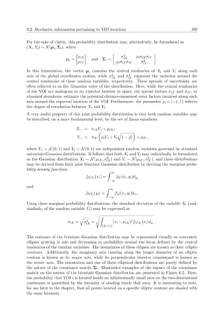
![110 Chapter 6. Management of stochastic information
xi
yi
(a) σ2
iX = 1 = σ2
iY t; ρi = 0
xi
yi
(b) σ2
iX = 1 = σ2
iY t; ρi = 0.25
xi
yi
(c) σ2
iX = 1 = σ2
iY t; ρi = −0.75
xi
yi
(d) σ2
iX = 1; σ2
iY t = 2; ρi = 0
xi
yi
(e) σ2
iX = 1; σ2
iY t = 2; ρi = 0.75
xi
yi
(f) σ2
iX = 2; σ2
iY t = 1; ρi = −0.25
Figure 6.2: Bivariate Gaussian probability distribution illustrations with different covariance matrices.
As ρi increases positively, the bivariate Gaussian distribution is stretched diagonally, forming
elliptical isopleths with positively sloped major axes. Conversely, as ρi increases negatively,
these isopleths are governed by negatively sloped major axes. Larger variance spreads stretch
the elliptic contours along their major and minor axes, and the smaller the variance of a random
variable is along its axis, the more “tightly peaked” the Gaussian bell in that dimension is.
The case in which these two random variables are uncorrelated or independent (i.e. whenever
ρi = 0) involves no apparent association between Xi and Yi. Intuitively, this is equivalent to
stating that no information is to be gained in investigating the “distance” from Xi to µiX by
knowing the value of Yi, and vice versa [163]. On the other hand, a strong correlation between
the two random variables suggests that the average “distance” of the pair (Xi, Yi) in the joint
probability distribution to the locus of central tendencies is expected to be rendered smaller by
this association. In other words, knowledge of one diminishes uncertainty in the other one for
cases in which these random variables are highly correlated.
Another benefit of adopting this probability distribution is that the isomorphism mapping points
from a real-life global coordinate system (e.g. a geodetic or polar coordinate system) to a more
simplified scale used for computing these probability distributions is both relatively simple and
one-to-one. For example, a coastal nation may wish to employ an isomorphism that converts
some real-life maritime coordinate system to a temporary, normalised, shifted local Cartesian
space for the purpose of efficiently computing response selection interception trajectories.
A significant drawback of adopting a bivariate Gaussian distribution to model the location of](https://image.slidesharecdn.com/6cd1ebf5-5cfe-4d40-998c-99cbe17b08f1-170109122537/85/PhD-dissertation-142-320.jpg)
![6.2. Stochastic information pertaining to VOI locations 111
objects in an MLE context, however, occurs in cases where VOIs are not cruising on the open
sea, but are rather moving close to land or other infeasible locations. In such cases, subsets of
the locations surrounding the expected location of a VOI will not be assigned zero probability
weights, although there really is a zero chance (with a few exceptions, such as amphibious
vehicles) that a VOI location will, at any point, be observed in such a subset. These cases
therefore require the implementation of alternative location modelling features.
6.2.2 On threat detection performance and VOI location uncertainty
As discussed in §3.1.1, threat detection systems are expected to transmit certain input data to
the MLE database in a specific format, and in a timely manner, via the attribute management
system. VOI coordinates at sea, VOI headings, VOI speeds and VOI predicted travel paths
are examples of such data. This information may then used as part of MLE response selection
operations in order, inter alia, to establish the feasible domain of a problem instance, detect
disturbances, and make necessary solution progression micro-adjustments. The reader is referred
to the work of du Toit [49] to gain some insight into the process of deriving threat detection
information related to location, movement and trajectory paths of VOIs.
This information transfer process may, however, significantly vary from one coastal nation to
another as a result of the different natures of MLE threat detection systems in place. Indeed,
as mentioned earlier, the ability of MLE response selection systems to receive adequate VOI
information in real time is significantly constrained by the ability of threat detection systems to
derive such information.
In order to achieve effective MLE response selection operations, real time VOI locations ought
to be pinpointed in space as accurately as possible with as little margin for error as possible, and
this is also critical when anticipating future VOI locations. The quality and level of resolution
of radars as well as their general distance from VOIs are examples of factors that may have an
impact on the level of uncertainty pertaining to VOI locations in real time. Examples of “weak”
and “competent” threat detection systems implemented toward modelling the probability dis-
tribution of the location of the same VOI at the same time is illustrated in Figure 6.3. Note
that this VOI location follows a bivariate Gaussian probability distribution. Here, it is easy to
see that the two univariate Gaussian bells are more stretched out in Figure 6.3 (a) as a result of
higher uncertainty around the corresponding marginal probability density function mean values,
µiX and µiY , which is an indication of lesser adequate threat detection systems.
Fortunately, there exist many effective techniques to consolidate the data obtained from obser-
vations made by various (independent) sources in order to predict the position of an object at
sea more accurately. This is particularly the case whenever a coastal nation has multiple radar
sources at its disposal that do not typically perform very well on their own (as illustrated in
Figure 6.3 (a)). The reader is referred to the work of Stroupe et al. [137] to gain insight into
how this is achieved. Here, object positions collected by multiple individually operated robots
are modelled as bivariate Gaussian distributions. A consolidation technique employed, called
the multi-distribution merging process, then merges these probability distributions as a means to
achieve greater effective sensor coverage of the environment, in turn improving the accuracy of
object position estimates. This technique is analogous to using multiple threat detection sources
as a way of assessing the estimated position of VOIs in real time. That is, information collected
from multiple points of view can reduce uncertainty, improve accuracy and tighten confidence
intervals. Another example of such a technique is the cooperative merging of several hundreds
of super-telescopes around Earth in order to improve the accuracy of images gathered in deep
outer space [155].](https://image.slidesharecdn.com/6cd1ebf5-5cfe-4d40-998c-99cbe17b08f1-170109122537/85/PhD-dissertation-143-320.jpg)
![112 Chapter 6. Management of stochastic information
E[(Xi, Yi)]
µiX µiY
fNXi
(xi)
fNYi
(yi)
yi xi
fN(xi,yi)
(a) Weak MLE threat detection systems result in
higher uncertainty with respect to the estimated
locations of VOIs in general.
E[(Xi, Yi)]
µiX µiY
fNXi
(xi)
fNYi
(yi)
yi xi
fN(xi,yi)
(b) Competent MLE threat detection systems re-
sult in higher accuracy with respect to the esti-
mated locations of VOIs in general.
Figure 6.3: An illustration of two different threat detection systems used to model the probability dis-
tribution of the location of (the same) VOI i along a two-dimensional coordinate system at a certain point
in time. Here, the joint probability density function fN (xi, yi) follows a bivariate Gaussian distribution
with corresponding univariate marginal probability density functions fN Xi
(xi) and fN Yi
(yi) projected
onto their respective planes.
6.3 Stochastic information pertaining to visitation locations
Although the information pertaining to VOI location tracking in real time discussed in the
previous section is important for use in MLE response selection operations, it is really only
important for trajectory adjustments on a micro-management level as well as for the detection
of sudden, unanticipated changes in VOI itineraries for use in problem instance reinitialisation
processes. For the purpose of configuring visitation routes, however, it is further required to
anticipate the locations of VOIs in the future, and this is unarguably of utmost importance.
Indeed, as described in Chapter 4, these anticipated locations are used in the mathematical
modelling process to compute visitation locations — points in space and time on the visitation
routes of active MLE resources where interception with the scheduled VOIs take place.
6.3.1 Anticipated VOI trajectories
Intuitively speaking, anticipated VOI locations may be thought of as 2-dimensional T-tuples
corresponding to the projections of the anticipated central tendencies of VOI i at specific time
instants, modelled as a time series {(Xi, Yi)t, t = 1, 2, . . . , T}, for all i ∈ Ve. This set is defined
here as an anticipated VOI trajectory — a time-ordered set of states of anticipated VOI locations
at various points in the future which are governed by bivariate Gaussian probability distributions.
Although the long term accuracy of predicting anticipated VOI locations is expected to be
relatively poor, it is nevertheless important that the pre-configured length of this time series
(i.e. the parameter T) be large enough to allow for MLE response selection operations involving
the estimation of interception points along MLE resource visitation routes. Trajectory micro-
adjustments may nevertheless be carried out accordingly by MLE resource operators in time
as the routes progress and the actual anticipated interception points with VOIs scheduled for](https://image.slidesharecdn.com/6cd1ebf5-5cfe-4d40-998c-99cbe17b08f1-170109122537/85/PhD-dissertation-144-320.jpg)
![6.3. Stochastic information pertaining to visitation locations 113
visitation become more pronounced (as these become progressively nearer in the future than
when they were assessed at the beginning of the time stage).
Anticipated VOI trajectories may typically be derived by various techniques that combine an
appropriate amount of relevant information for best predictability. Such information may in-
clude, for example, the estimated size, current location and current velocity of the VOI, together
with its historical trajectory and speculations in respect of its possible activities and intentions
at sea. As mentioned in §6.2, however, the level of accuracy of anticipated VOI trajectories
will, in general, greatly depend on the accuracy of threat detection systems and expertise of
operators to perform these tasks. This problem is often complicated in real life as the expected
future location of a VOI may typically only be known indirectly through a sequence of relative
frames of reference with increasing uncertainty [6].
Examples of techniques employed in the literature to derive anticipated VOI trajectories include
multi-modal Gaussian mixture models [6] and hidden Markov models [49]. An in-depth analysis
of anticipated VOI trajectories is outside the scope of this dissertation. Based on what was
uncovered in the literature, it is, nevertheless, necessary to acknowledge that this undertaking is
by no means a trivial task. It is therefore assumed in the remainder of this chapter that threat
detection systems are able to derive this information to a certain degree of predictability and
make it available to the MLE response selection DSS in real time.
6.3.2 On the representation of anticipated VOI velocity vectors
Similarly to predicting VOI locations in real time, deriving anticipated VOI velocities should
ideally be carried out by combining various techniques as a means to achieve maximum efficiency.
Such techniques include polynomial and spline interpolation [161], compound approximate trans-
formations [132], Bayesian time series analysis (for the evaluation of posterior probability dis-
tributions) [121] and dynamic time warping [49]. An in-depth analysis of these a processes
is, once again, beyond the scope of this dissertation. The focus in this section is rather on
the presentation of various useful formats in which MLE threat detection systems may model
anticipated VOI velocity vectors for use in MLE response selection operations.
Because these velocity vectors are not characterised with explicit sets of parameters (except for
the chronological progression of the object at points on a time line), their derivation resides in the
modelling realm of non-parametric modelling [132]. Perhaps the most appropriate mathematical
modelling approach towards determining the chronological progression of such objects in both
space and time involves the derivation of pairs of parametric expressions in terms of a time
parameter, such that each of these expressions represents the anticipated progression of a VOI
as a function of time with respect to one of two global axes. This is a useful representation, as
these expressions will simultaneously also express the anticipated locations of VOIs over time.
Three general styles of anticipated VOI velocity vector representations are presented in the
remainder of this section. If the anticipated rate of change of displacement of a VOI over
a pre-defined period of time is fixed, then its velocity vector representation is referred to as
static. On the other hand, a velocity vector representation is said to be dynamic if the VOI is
expected to change speed or direction at any point in the near-future. The choice of velocity
vector representation will typically vary based on subjective preference of operators, quantity
of historical locations data gathered, operators expertise and general prediction capabilities and
accuracy of the threat detection system models.](https://image.slidesharecdn.com/6cd1ebf5-5cfe-4d40-998c-99cbe17b08f1-170109122537/85/PhD-dissertation-145-320.jpg)
![114 Chapter 6. Management of stochastic information
Static representation of velocity vectors
Two methods of static anticipated VOI velocity vectors are presented here. The first involves
treating the rate of change of displacements along each of two global axes independently, that
is defining VOI i’s anticipated velocity vector ˜vi = [ςix ςiy], where ςix is the anticipated (fixed)
speed component along the x-axis and ςiy is the anticipated speed component along the y-axis.
The anticipated location of this VOI as a function of time with respect to the global frame of
reference is given by
(xi(t), yi(t)) = (xi(0) + tςix, yi(0) + tςiy).
The second method of static velocity vector representation involves assessing the estimated
heading θi of VOI i with respect to a global x-axis together with its estimated speed ςi relative
to the plane in order to form the vector ˜vi = [θi si]. This representation is particularly useful
from a visual point of view on operator screens, where a vector arrow may point out of the
VOI such that the direction of this arrow is governed by θi and such that its length is directly
proportional to ςi. In this representation, the anticipated location of the VOI as a function of
time with respect to the global frame of reference is given by
(xi(t), yi(t)) = (xi(0) + tςi cos θi, yi(0) + tςi sin θi).
Although static velocity vector representations are relatively easy to configure, they are most
likely not a very accurate representation of reality2, particularly if the time period over which
estimates of the velocity of the VOI is performed is long. This representation nevertheless works
best when few data points are available and linear interpolation is the best available option to
predict the movement of VOIs.
Dynamic representation of velocity vectors
Alternatively, it is advocated that parametric representations of the anticipated velocity vectors
of VOIs be configured more generically by means of higher-degree polynomials (i.e. preferably
such that at least one of the two vector components be at least quadratic). For example, let the
anticipated location of VOI i as a function of time be given by
(xi(t), yi(t)) = (ai0 + ai1t + ai2t2
+ . . . + aiNix tNix
, bi0 + bi1t + bi2t2
+ . . . + biNiy tNiy
),
where ai0, . . . , aiNx and bi0, . . . , biNy are real coefficients. In the case where Nix = 1 = Niy, the
representation conforms to the formulation of the first type of static velocity vector representa-
tion discussed above, where ai1 = six and bi1 = siy. Of course, the case where Nix = 0 = Niy
suggests the presence of an immobile VOI.
Given a set of parametric expressions in such a format, its corresponding anticipated VOI velocity
vector as a function of time is given by
˜vi(t) =
dxi(t)
dt
dyi(t)
dt
.
Moreover, one may also wish to derive the anticipated speed and acceleration vector of the VOI
as a function of time for use in MLE response selection operations. Its speed component at any
2
The level of accuracy of the VOI velocity prediction models can be measured retrospectively by comparing
the a priori anticipated VOI trajectory with its a posteriori trajectory path using appropriate metrics such as
measuring the sum of the areas enclosed between the two curves over a pre-defined finite period of time.](https://image.slidesharecdn.com/6cd1ebf5-5cfe-4d40-998c-99cbe17b08f1-170109122537/85/PhD-dissertation-146-320.jpg)
![6.3. Stochastic information pertaining to visitation locations 115
given time is then easily computed as
||˜vi(t)|| =
dxi(t)
dt
2
+
dyi(t)
dt
2
,
while its bearing component is derived using the arc tangent function
˜θi(t) = arctan
dyi(t)
dt
dxi(t)
dt
−1
∈ [−π, π]
and its acceleration vector is simply
˜ai(t) =
d2xi(t)
dt2
d2yi(t)
dt2
.
Step function representation
To avoid the difficulties that may accompany the evaluation of higher-degree polynomials, as well
as possibly improving prediction accuracy, an anticipated VOI velocity vector may, alternatively,
be broken down into a step function consisting of a time sequence of pre-defined lower-degree
polynomials. This is particularly useful in cases where the VOI is strongly expected to experience
sudden significant changes in direction and/or velocity at specific points in the future. Such
predictions may, for example, be the result of certain geographical or environmental features
crossing paths with the anticipated trajectory of the VOI, or of the known threatening activities
and intentions of the VOI that give away clear indications as to where it is expected to make
sudden dramatic changes in velocity.
Such an anticipated VOI velocity representation may be expressed as a continuous sequence of Ξ
consecutive anticipated VOI velocity vectors defined over specific time intervals [0, t1], [t1, t2], . . . ,
[tT−1, Ξ], that is
˜vi(t) =
˜v1
i (t) , if 0 ≤ t ≤ t1,
˜v2
i (t) , if t1 ≤ t ≤ t2,
...
...
˜vΞ
i (t) , if tΞ−1 ≤ tΞ.
6.3.3 Uncertainty factors pertaining to anticipated VOI locations
In this section, a discussion is conducted on the major factors impacting the estimated level
of uncertainty of anticipated VOI locations. Overall, a trade-off has to be found between the
extent to which these errors may be accounted for and the rate at which new problem instances
are triggered (i.e. time stage termination) due to unforeseen input data deviations caused by
these factors. In particular, it is required to assess the potential extent of influence of such
changes on the quality of a currently implemented solution. It is expected that the following six
factors may influence the intensity of noise whilst in the process of configuring the probability
distributions corresponding to the set of anticipated VOI locations {(Xi, Yi)t}:
1. The performance level of threat detection external infrastructure,
2. The performance level of threat detection systems in the derivation of anticipated VOI
velocity vectors,](https://image.slidesharecdn.com/6cd1ebf5-5cfe-4d40-998c-99cbe17b08f1-170109122537/85/PhD-dissertation-147-320.jpg)
![6.3. Stochastic information pertaining to visitation locations 117
and/or significant unpredicted rates of change of velocity along their historical tracks, or high
uncertainty with respect to the type of threat(s) that some VOIs are speculated to embody, in
turn causing its future whereabouts to be more speculative as well.
Finally, Factor 6 relates to the actual nature of the anticipated velocity vector assigned to a VOI
and, in particular, to its anticipated speed component. More specifically, slight unanticipated
bearing deviations from the anticipated bearing vector component (˜θi(t)) and, consequently,
from the anticipated VOI locations, are expected to have a larger impact on the margin of error
in anticipated VOI locations over a specific time frame whenever VOIs navigate at relatively
high speeds. As a result, there may exist a positive correlation between the anticipated speed
of a VOI and its anticipated location uncertainty in the future.
6.3.4 Derivation of anticipated VOI location probability distributions
For the purpose of enforcing the abstract link between MLE threat detection and MLE response
selection systems, it is important to step slightly outside the scope of this dissertation and
elaborate briefly on the process according to which threat detection systems may be able to derive
the probability distributions associated with the anticipated locations of VOIs. While the central
tendencies of these distributions may be derived with relative ease from the anticipated VOI
velocity vectors (or, analogously, from the anticipated VOI location parametric representations,
as discussed in §6.3.2), deriving the parameter estimators representing the degree of uncertainty
around these central tendencies forms another thick layer of complexity to the already highly-
stochastic nature of the MLE response selection problem. The focus in the remainder of this
section will therefore evolve around determining such estimators in a format that is both realistic
and adequate to the formulation of stochastic MLE response selection model components.
In §6.2.1, it was suggested that the stochastic representation of the real time locations of VOIs
may be modelled effectively according to a bivariate Gaussian probability distribution. Following
this suggestion, consider the pair of random variables (Xi, Yi)t ∼ N(µit, Σit) with probability
density function fN (xi, yi)t, for all t ∈ {1, 2, . . . , T}. It is important to note that the consoli-
dation µit = E[(Xi, Yi)t] = (xi(t), yi(t)) between the anticipated VOI locations and its future
(Gaussian) central tendencies follows as a result of this construction. Moreover, from Factor
3 in §6.3.3, it is agreed that the condition σix(t+1) > σixt and σiy(t+1) > σiyt must hold for
all t ∈ {0, . . . , T − 1} in general, where σixt and σiyt are the anticipated standard deviations
associated with the random variables (Xi, Yi)t.
The derivation of the associated distribution covariance matrix is conducted next. Perhaps
the most effective way in which threat detection systems are able to model the uncertainty
surrounding the location of a VOI at some point in the future according to a bivariate Gaussian
probability distribution is to orientate the major axes of its underlying elliptic contours in
alignment with the anticipated velocity of the VOI a that time. It follows that the bearing of
the VOI will always be aligned to the major axis of its Gaussian distribution at that time in
such a configuration.
Moreover, it may be convenient to model the anticipated central tendencies and Gaussian noise
of the VOI in respect of a strategic two-dimensional temporal local set of coordinate axes,
or local frame of reference. To this end, it is proposed that the local frame of reference be
modelled with the ordered basis {˘xit∗ , ˘yit∗ } configured in such a way as to have the local x-axis
and y-axis parallel and perpendicular to the bearing of the anticipated VOI velocity at time
t∗ ≥ 0, respectively. A visual representation of this construction is illustrated in Figure 6.4.
This particular choice of local axes has the benefit of avoiding any correlation between the
two random variables ˘Xit∗ and ˘Yit∗ , which is a difficult aspect of the distribution covariance](https://image.slidesharecdn.com/6cd1ebf5-5cfe-4d40-998c-99cbe17b08f1-170109122537/85/PhD-dissertation-149-320.jpg)
![118 Chapter 6. Management of stochastic information
that threat detection systems therefore need not concern themselves with. This local bivariate
Gaussian distribution may therefore be modelled as ( ˘Xit∗ , ˘Yit∗ ) ∼ N(˘µit∗ , ˘Σ), where ˘µit∗ = µit∗
and
˘Σit∗ =
˘σ2
iXt∗ 0
0 ˘σ2
iY t∗
. (6.1)
In (6.1), the values ˘σ2
iXt∗ and ˘σ2
iXt∗ represent the estimated error margins along the ˘xit∗ and ˘yit∗
axes (the major and minor axes of this distribution), respectively.
xi
yi
˘x
it∗
˘yit∗
E[(Xi, Yi)t∗] = (xi(t∗
), yi(t∗
))
E[vi(t∗
)]
θi(t∗
)
π
2
(xi(0), yi(0))
Figure 6.4: A bivariate Gaussian probability distribution relative to a local set of coordinates.
For use in MLE response selection operations, however, it is necessary to transform this proba-
bility distribution representation of anticipated VOI locations to the global frame of reference,
referred to here as its canonical form. In their research, Smith et al. [132] defined an uncer-
tainty transformation as an estimated mean relation of one local coordinate frame relative to
some defining global coordinate frame together with a covariance matrix that expresses the
uncertainty of such an estimate.
Transforming the probability distribution from this local frame to its canonical form may be
achieved via a linear isomorphism procedure. It is easy to see that such a transformation may
be achieved by performing a rotation of −θit∗ radians of all points around the central tendencies
of the distribution, which corresponds to an angular rotation of the covariance matrix in which
the parameter ρit allows for the major and minor axes of a Gaussian ellipse to be rotated. This
rotation isomorphism may be achieved by means of the two-by-two matrix
W =
cos θit∗ sin θit∗
− sin θit∗ cos θit∗
with transpose
WT
=
cos θit∗ − sin θit∗
sin θit∗ cos θit∗
.
By computing the Jacobian matrix of the transformation equations and employing the properties
of eigenvectors, the identity
[xi yi] Σ−1 xi
yi
= [xi yi] WT ˘Σ
−1
W
xi
yi](https://image.slidesharecdn.com/6cd1ebf5-5cfe-4d40-998c-99cbe17b08f1-170109122537/85/PhD-dissertation-150-320.jpg)
![6.3. Stochastic information pertaining to visitation locations 119
holds true for all transformations of this type [107, 132, 137], where (xi, yi) is a vector of random
variables governed by a bivariate Gaussian probability distribution3. It is a well-known fact that
WT
= W−1
[132]. The transformation of the local covariance matrix to its canonical form is therefore given
by
Σ = WT ˘Σ
−1
W
−1
= ˘Σ
−1
W
−1
(WT
)−1
= W−1 ˘Σ
−1 −1
WT −1
= W−1 ˘Σ WT −1
= WT ˘Σ W−1 −1
= WT ˘ΣW.
It follows that
Σ =
− cos θit∗ sin θit∗
− sin θit∗ − cos θit∗
˘σ2
iXt∗ 0
0 ˘σ2
iY t∗
− cos θit∗ − sin θit∗
sin θit∗ − cos θit∗
=
−˘σ2
iXt∗ cos θit∗ ˘σ2
iY t∗ sin θit∗
−˘σ2
iXt∗ sin θit∗ −˘σ2
iY t∗ cos θit∗
− cos θit∗ − sin θit∗
sin θit∗ − cos θit∗
=
˘σ2
iXt∗ cos2 θit∗ + ˘σ2
iY t∗ sin2
θit∗ (˘σ2
iXt∗ − ˘σ2
iY t∗ ) sin θit∗ cos θit∗
(˘σ2
iXt∗ − ˘σ2
iY t∗ ) sin θit∗ cos θit∗ ˘σ2
iXt∗ sin2
θit∗ + ˘σ2
iY t∗ cos2 θit∗
.
The variances of this distribution in respect of the global frame of reference are therefore given
by
σ2
iXt∗ = Σ11 = ˘σ2
iXt∗ cos2
θit∗ + ˘σ2
iY t∗ sin2
θit∗ , (6.2)
σ2
iY t∗ = Σ22 = ˘σ2
iXt∗ sin2
θit∗ + ˘σ2
iY t∗ cos2
θit∗ . (6.3)
Moreover, the correlation between the random variables Xit∗ and Yit∗ is given by the coefficient
ρit∗ =
Σ12
σiXt∗ σiY t∗
=
Σ21
σiXt∗ σiY t∗
=
(˘σ2
iXt∗ − ˘σ2
iY t∗ ) sin θit∗ cos θit∗
˘σ2
iXt∗ cos2 θit∗ + ˘σ2
iY t∗ sin2
θit∗ ˘σ2
iXt∗ sin2
θit∗ + ˘σ2
iY t∗ cos2 θit∗
.
(6.4)
6.3.5 A worked example
In order to validate the modelling approach described above for mapping the Gaussian noise
around the central tendencies of anticipated VOI locations, a numerical example representing a
hypothetical scenario is presented in this section.
3
Interestingly, a higher proportion of similar research endeavors focus on the converse of this problem, in which
the probability distribution of an object relative to a global frame of reference is required to be converted into a
local one in order to obtain a diagonal covariance matrix.](https://image.slidesharecdn.com/6cd1ebf5-5cfe-4d40-998c-99cbe17b08f1-170109122537/85/PhD-dissertation-151-320.jpg)
![120 Chapter 6. Management of stochastic information
Consider the ith VOI whose anticipated trajectory has to be mapped in time and space over a
three-hour period at regular half-hour intervals. Suppose that, based on historical information
associated with the VOI, threat detection systems are able to estimate its anticipated velocity
vector as
˜vi(t) = (5.4; −1.04t) ,
where each vector component is measured in nautical miles per hour or knots. If the estimated
position of the VOI with respect to the global frame of reference at time t = 0 is (535, 104.7),
the anticipated location of this VOI as a function of time is then given by
˜i(t) = 535 + 5.4t; 104.7 − 0.52t2
,
its anticipated speed as a function of time is given by
||˜vi(t)|| = 29.16 + 1.08t2,
and its anticipated acceleration vector by
˜ai(t) = (0, −1.04).
Although the acceleration is constant, it does not mean the VOI is expected to accelerate
constantly for three hours in a row. The parametric equation along the y-axis is nevertheless
quadratic, thus merely suggesting that the VOI’s rate of change of displacement along this axis
is not expected to be constant during the course of the three hour period, but rather “ever so
slightly” increasing over time. These data are tabulated in Table 6.1.
Time series ˜i(t) ˜vi(t) ||˜vi(t)|| ˜θi(t) ˜ai(t)
(Xi, Yi)0 (535, 104.70) (5.4; 0.00) 5.40 0 (0, −1.04)
(Xi, Yi)0.5 (537.7, 104.57) (5.4; −0.52) 5.42 −5.49 (0, −1.04)
(Xi, Yi)1 (540.4, 104.18) (5.4; −1.04) 5.50 −10.90 (0, −1.04)
(Xi, Yi)1.5 (543.1, 103.53) (5.4; −1.54) 5.62 −16.11 (0, −1.04)
(Xi, Yi)2 (545.8, 102.62) (5.4; −2.08) 5.79 −21.07 (0, −1.04)
(Xi, Yi)2.5 (458.5, 101.45) (5.4; −2.60) 6.00 −25.71 (0, −1.04)
(Xi, Yi)3 (551.2, 100.02) (5.4; −3.12) 6.24 −30.02 (0, −1.04)
Table 6.1: Anticipated VOI characteristics in the form of a time series {(Xi, Yi)t}.
Suppose that these anticipated VOI locations are each modelled as bivariate Gaussian probability
distributions with respect to some temporary local sets of axes, constructed as described in §6.3.4.
In addition, suppose that the threat detection systems are able to predict the Gaussian noise
with respect to the local frame of references (namely the parameters ˘σ2
iXt∗ and ˘σ2
iY t∗ ) around
the anticipated locations in the time series {(Xi, Yi)t} as shown in Table 6.2. The results of
applying (6.2)–(6.4) are also shown in Table 6.2. These results were computed in the software
package MATLAB [147]. A visualisation of the resulting time series of anticipated VOI locations
is provided in Figure 6.5.
6.3.6 The dynamic bivariate Gaussian probability distribution
While an effective procedure for modelling the anticipated locations of a VOI defined by the
elements of the discrete set {(Xi, Yi)t} was proposed in the previous section, it is duly acknowl-
edged that, given the nature of the routing models of Chapter 4, VOI interception trajectories](https://image.slidesharecdn.com/6cd1ebf5-5cfe-4d40-998c-99cbe17b08f1-170109122537/85/PhD-dissertation-152-320.jpg)
![6.3. Stochastic information pertaining to visitation locations 121
Time series µiX µiY ˘σ2
iXt ˘σ2
iY t ˘ρi σ2
iXt σ2
iY t ρi
(Xi, Yi)0 535.0 104.70 1.0 0.6 0 1.00 0.60 0.00
(Xi, Yi)0.5 537.7 104.57 2.0 1.0 0 1.99 1.01 −0.071
(Xi, Yi)1 540.4 104.18 2.2 1.1 0 2.16 1.14 −0.130
(Xi, Yi)1.5 543.1 103.53 2.4 1.2 0 2.31 1.29 −0.185
(Xi, Yi)2 545.8 102.62 2.6 1.3 0 2.43 1.47 −0.231
(Xi, Yi)2.5 548.5 101.45 2.8 1.4 0 2.54 1.66 −0.266
(Xi, Yi)3 551.2 100.02 3.0 1.5 0 2.62 1.88 −0.293
Table 6.2: Bivariate Gaussian probability distribution parameters (with respect to both the local and
global frames of reference) corresponding to the kinematic data in Table 6.1.
xi
yi
98
99
100
101
102
103
104
105
535 536 537 538 539 540 541 542 543 544 545 546 547 548 549 550 551 552 553
E[(Xi, Yi)3]
E[(Xi, Yi)2.5]
E[(Xi, Yi)2]
E[(Xi, Yi)1.5]
E[(Xi, Yi)1]
E[(Xi, Yi)0.5]E[(Xi, Yi)0]
˜i(t)
Figure 6.5: Visualisation of the anticipated trajectory of VOI i over the time series of an-
ticipated locations (Xi, Yi)0, . . . , (Xi, Yi)3 in Table 6.2 with respective probability distributions
N(µi0, Σi0), . . . , N(µi3, Σi3).
actually have to be calculated in the space-time continuum in the form of a shortest set of rout-
ing arcs. In other words, for the sake of practicality of MLE response selection computations,
the parameter 0 ≤ t ≤ T should rather be defined on R in the time series {(Xi, Yi)t}, because
MLE response selection computations are not possible based solely on the location distribution
of an estimated scheduled interception time.
In §6.3.2, it was hinted that an anticipated VOI velocity vector may be obtained from a contin-
uous mapping of anticipated VOI locations obtained from the anticipated trajectory (or antic-
ipated system tracks) of the VOI calculated by MLE threat detection systems. This function
of anticipated VOI locations is depicted in Figure 6.5 in the context of the worked example
and is denoted by a vector ˜i(t). It is thus assumed that the expected central tendencies
E[(Xi, Yi)t] = ˜i(t) are known for all t ∈ [0, T].
In order to address the issue of expressing the anticipated position of a VOI as well as the
level of uncertainty surrounding that anticipated position over a time continuum, however, de-
fine the dynamic bivariate Gaussian probability distribution of the random variables (Xi, Yi)t as
(Xi, Yi)t ∼ (µiX(t), µiY (t), σ2
iX(t), σ2
iY (t), ρi(t)) or (Xi, Yi)t ∼ N(µi(t), Σi(t)). Note the differ-
ence in notation from the discrete formulation N(µit, Σit), in the sense that this distribution](https://image.slidesharecdn.com/6cd1ebf5-5cfe-4d40-998c-99cbe17b08f1-170109122537/85/PhD-dissertation-153-320.jpg)
![122 Chapter 6. Management of stochastic information
is now defined as a continuous function of time and. Here, as discussed above, the anticipated
VOI location vector
˜i(t) = (xi(t), yi(t)) = E[(Xi, Yi)t] = µi(t) =
µiX(t)
µiY (t)
may be thought of as an adequate estimator of the function of the central tendencies of this
distribution. Moreover, the estimator functions ˘σ2
iX(t) and ˘σ2
iY (t) are defined similarly as in
§6.3.4 to model the expected growth in uncertainty relative to the anticipated velocity vector
of the VOI expressed in terms of temporary frames of reference, from where the distribution
uncertainty parameters may be derived in canonical form. It follows from (6.2)–(6.4) that
σ2
iX(t) = ˘σ2
iX(t) cos2
θi(t) + ˘σ2
iY (t) sin2
θi(t), (6.5)
σ2
iY (t) = ˘σ2
iX(t) sin2
θi(t) + ˘σ2
iY (t) cos2
θi(t) (6.6)
and
ρi(t) =
sin θi(t) cos θi(t)(˘σ2
iX(t) − ˘σ2
iY (t))
˘σ2
iX(t) cos2 θi(t) + ˘σ2
iY (t) sin2
θi(t) ˘σ2
iX(t) sin2
θi(t) + ˘σ2
iY (t) cos2 θi(t)
. (6.7)
To demonstrate the working of this parametric multivariate distribution, reconsider the example
of §6.3.5. Of course, by assumption,
µi(t) =
535 + 5.4t
104.7 − 0.52t2 .
The variance functions in terms of the global frame of reference can, in essence, be estimated in
two different ways. On the one hand, these noise functions may be expressed in the form of the
continuous step functions
˘σ2
iX(t) =
1 + 2t , if 0 ≤ t ≤ 0.5
1.8 + 0.4t , if 0.5 ≤ t ≤ 3
and
˘σ2
iX(t) =
0.6 + 0.8t , if 0 ≤ t ≤ 0.5
0.9 + 0.2t , if 0.5 ≤ t ≤ 3
in terms of the local frame of reference. The dynamic covariance function with respect to the
global frame of reference may then be computed according to (6.5)–(6.7). The second method
consists of using polynomial interpolation in order to find a continuous function that best fits the
estimated (global) variances derived in the discrete case. Using the values derived in Table 6.2,
the variance function over the time interval [0, 3] along the global x-axis may best be estimated
by the fifth-degree polynomial
σ2
iX(t) ≈ 0.1t5
− 0.92t4
+ 3.06t3
− 4.77t2
+ 3.69t + 1,
while the variance function over the time interval [0, 3] along the global y-axis may best be
estimated by the fourth-degree polynomial
σ2
iY (t) ≈ −0.05t4
+ 0.39t3
− 0.93t2
+ 1.15t + 0.6.](https://image.slidesharecdn.com/6cd1ebf5-5cfe-4d40-998c-99cbe17b08f1-170109122537/85/PhD-dissertation-154-320.jpg)
![6.3. Stochastic information pertaining to visitation locations 123
6.3.7 Confidence ellipses
As described earlier, a multivariate Gaussian probability distribution elliptic contour comprises
a region of random variable value combinations (defined within an infinitesimally small area)
so that each random variable has an identical chance of being observed. An elliptic contour is,
however, mostly thought of as bounding a measurable set (in this case a probabilistic subspace
measured in the interval (0, 1)) containing a specific subset of random variable value combina-
tions distributed around the central tendencies of the underlying Gaussian distribution. These
random variable values are then said to possess identical Mahalanobis distances [98] and, in cases
where the random variables are uncorrelated, this metric may be simplified to a normalised Eu-
clidean distance. These contours are often called confidence ellipsoids for practical reasons, or
confidence ellipses in the bivariate case.
Formally speaking, α-bounded confidence ellipsoids represent values for the population param-
eter vector µi for which the difference between these parameter values and the (a posteriori)
observed estimate is not statistically significant at the 1 − α % level [75], where α, typically
defined in the interval (0.80, 1), is the desired level of confidence prescribed by the decision
maker. This probability bound may therefore be thought of as an indicator of the reliability of
the estimation procedure rather than as some specific pre-calculated interval.
Without loss of generality, all time-related subscripts in this description of confidence ellipses are
omitted from the parameters. For the sake of lucidity, it is beneficial to first analyse confidence
ellipses mapped in the domain space of uncorrelated bivariate Gaussian random variables. In
this simplified case, the lengths of the principal axes of the confidence ellipse may be defined
solely in terms of the standard deviations σ2
iX and σ2
iY . The equation of the ellipse is given by
xi − µiX
σ2
iX
2
+
yi − µiY
σ2
iY
2
= Φi,
where the parameter Φi represents a positive real number defining the scale of the ellipse with
respect to the underlying Gaussian distribution. A question arises as to how this parameter
should be configured so that the resulting elliptic contour precisely matches a pre-established
confidence level α. Because the random variables Xi and Yi are uncorrelated, the sum of the left
hand side of the equation above represents the sum of squares of two independently Gaussian
distributed random variables. It is known that the sum of squared Gaussian random variables
is distributed according to the Chi-Square probability distribution [133], so it follows that the
parameter Φi may be assessed accordingly by calculating the corresponding Chi-Square likeli-
hood with two degrees of freedom (i.e. one for each unknown). Moreover, as suggested earlier,
confidence ellipses may be described as the accumulated probabilities of all infinitesimally small
regions contained inside this ellipse, and this is analogous to accumulating all points on these
infinitely many ellipses of monotonically decreasing scales that are bounded above by the confi-
dence ellipse of scale Φi. In other words, P Φi < χ2
α(2) = α, where χ2
α(2) represents the upper
critical value4 of the Chi-Square distribution with two degrees of freedom and a confidence ellipse
bounded by the parameter α. Informally speaking, an α% confidence interval may therefore be
thought of as related to the value χ2
α(2) in such a way that α% of the distribution density is
bounded inside the ellipse
xi − µiX
σ2
iX
2
+
yi − µiY
σ2
iY
2
= χ2
α(2).
Finally, by definition of the ellipse in the context of analytical geometry, the lengths of the
principal axes of a confidence ellipse are 2σiX χ2
α(2) and 2σiY χ2
α(2).
4
These values may be found in any Chi-Square probability tables [107].](https://image.slidesharecdn.com/6cd1ebf5-5cfe-4d40-998c-99cbe17b08f1-170109122537/85/PhD-dissertation-155-320.jpg)
![124 Chapter 6. Management of stochastic information
The case for which the random variables are correlated is now considered. Here, the resulting
confidence ellipses will not be axes-aligned with respect to the global reference coordinate frame.
The eigenvectors of the covariance matrix5 of a bivariate Gaussian distribution correspond to
the principal directions of the distribution, while its eigenvalues correspond to the degrees of
spread induced by the variances along the corresponding directions [107]. In other words, the
eigenvectors of the covariance matrix of the underlying Gaussian distribution represent the
direction of the error vectors along the largest spread of density points (namely along the major
and minor axes of the ellipse), while the eigenvalues represent the magnitude of error with
respect to the corresponding vectors. Numerically speaking, the lengths of the principal axes of
the rotated confidence ellipse are given by 2 χ2
α(2)λ1 and 2 χ2
α(2)λ2, where λ1 and λ2 are the
eigenvalues of the covariance matrix. For consolidation and validation purposes (with regard
to the local frames of reference derived in §6.3.4), it is useful to observe at this point that the
orientation of a correlated confidence ellipse with respect to the global x-axis is arctan(wλ1 w−1
λ2
),
where wλ1 is the eigenvector of the covariance matrix corresponding to the largest eigenvalue
(i.e. the eigenvalue associated with the major axis of the confidence ellipse) [133].
6.3.8 Discussion
The aim in this section was to propose a method for configuring stochastic input data pertaining
to anticipated VOI locations into a framework that is both feasibly tractable from the stand-
point of MLE threat detection systems and directly applicable to routing operations from the
standpoint of MLE response selection systems. This was achieved in such a way that the output
information of the former system forms a direct bridge with the input data of the latter. First, it
was argued in §6.2 that it would be unrealistic to model the calculated interception points with
VOIs in space deterministically. The bivariate Gaussian probability distribution was therefore
introduced as a means of capturing the stochastic aspect of this calculation, and its adequacy
to fulfill this task in the context of MLE response selection operations was motivated.
In §6.3.2 it was suggested that the central tendencies of the anticipated locations of a VOI at
future points in time may be modelled within the current time stage by considering the points
mapped by the anticipated trajectory derived from a pre-determined anticipated VOI velocity
vector. A discussion on various factors that may contribute to the magnitude of the VOI
locations Gaussian noise in an MLE environment was conducted in §6.3.3. Thereafter, it was
demonstrated in §6.3.4 and §6.3.5 that it may be possible to express the uncertainty surrounding
the expected location of a VOI at some point in the future by considering two perpendicular error
vectors aligned with the major and minor axes of this anticipated VOI location in such a way
as to consider the eigenvector corresponding to the major axis analogously to the (anticipated)
heading vector of the VOI at that point in time via a local frame of reference. Because MLE
response selection systems plan visitation routes along a time-continuum, discrete anticipated
VOI location probability distributions may not be appropriate, leading to the definition of the
dynamic bivariate Gaussian distribution in §6.3.6 in order to address this issue. The notion of
confidence ellipses was finally introduced in §6.3.7 as a means to bound these bivariate Gaussian
distributions from above. The concepts of the dynamic bivariate Gaussian distribution and
confidence ellipses will be brought together later in the dissertation for the purpose of defining so-
called hyper-dimensional Gaussian corridors. These corridors may be used to configure problem
instance reinitialisation protocols (disturbance triggering conditions) pertaining to “significant”
deviations in actual VOI velocity vectors relative to VOI velocity vectors anticipated a priori.
5
The eigenvalues of a covariance matrix may easily be calculated from the familiar characteristic equation
det(Σ − λI) = 0.](https://image.slidesharecdn.com/6cd1ebf5-5cfe-4d40-998c-99cbe17b08f1-170109122537/85/PhD-dissertation-156-320.jpg)
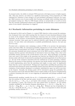
![126 Chapter 6. Management of stochastic information
6.4.1 On the probability distribution of route distances
Consider the characteristic function7
φz(ω) = E[e−ωιz] = e(ι ωT µ−ωT Σω)
of two random variables (X, Y ) ∼ N(µ, Σ), where ι is the imaginary unit
√
−1 and ω ∈ R2
is the so-called argument vector of the characteristic function. Moreover, consider the two
independent8 bivariate Gaussian random variables vectors zi = (Xi, Yi) ∼ N(µi, Σi) and zj =
(Xj, Yj) ∼ N(µj, Σj), where i, j ∈ {0, 1, . . . , n, n+1} and |i−j| = 1. Then, considering that the
sum of two independent random variables is, in fact, the product of their respective characteristic
functions and acknowledging that the random variable z has the same covariance as the random
variable −z, but with opposite means [95], it follows that
φ(zi−zj)(ω) = e(ι ωT µi−ωT Σiω)
e(−ι ωT µj−ωT Σjω)
= e(ι ωT µi−ωT Σiω−ι ωT µj−ωT Σjω)
= e(ι ωT (µi−µi)−ωT (Σi+Σj)ω)
,
and so (zi − zj) ∼ N(µi − µj, Σi + Σj). If d = (zi − zj) ∼ N(µd, Σd), then
µd =
µiX − µjX
µiY − µjY
and
Σd =
σ2
iX ρiσiXσiY
ρiσiXσiY σ2
iY
+
σ2
jX ρjσjXσjY
ρjσjXσjY σ2
jY
=
σ2
iX + σ2
jX ρiσiXσiY + ρjσjXσjY
ρiσiXσiY + ρjσjXσjY σ2
iY + σ2
jY
.
Moreover, the squared Euclidean distance between zi and zj is given by dT
d = (zi − zj)T (zi −
zj). But this also corresponds to the inner product d, d in R2 and, while the product of two
bivariate Gaussian distributions may not be normalised as a density of the underlying vector of
random variables [112], computing the probability distribution of this inner product is perfectly
plausible since both distributions are identical and thus of the same dimension. The interested
reader is referred to [77, 97, 112, 144] for discussions on the probability distributions of the
product of multivariate Gaussian probability distributions. Given these identical distributions,
the probability density functions may be expressed as
dT
d ∼ N(µd, Σd), N(µd, Σd)
∼ N(Σd(Σd + Σd)−1
µd + Σd(Σd + Σd)−1
µd, Σd(Σd + Σd)−1
Σd)
∼ N(2Σd(2Σd)−1
µd, Σd(2Σd)−1
Σd).
This result suggests that the square distance between two Gaussian distributed bivariate random
variables is itself, in fact, Gaussian (univariate, of course). Moreover, since there exists a one-to-
one correspondence between the characteristic function and cumulative distribution functions
7
A characteristic function provides an alternative way of describing a random variable. If a random variable is
governed by a density function, then the characteristic function is its dual in the sense that each of these functions
is a Fourier transformation of the other [75].
8
With respect to one another, that is, but not necessarily with respect to the correlation status of their
respective individual random variables.](https://image.slidesharecdn.com/6cd1ebf5-5cfe-4d40-998c-99cbe17b08f1-170109122537/85/PhD-dissertation-158-320.jpg)
![6.4. Stochastic information pertaining to route distances 127
of a random variable, it is always possible to derive one of these functions from the other one.
According to Kettani and Ostrouchov [77], the characteristic function of this probability density
function is given by
φdT
d(ω) =
exp tr{−ωι(I + 2ωιΣd)−1µT
d µd}
|I + 2ωιΣd|
,
where ω ∈ R is the argument of the characteristic function and the function tr{.} represents
the trace of a matrix (i.e. the sum of its main diagonal entries). Simplified probability density
functions for special cases of the bivariate normal distribution are also derived in [77]. The
random variable dT
d has, for example, been shown to assume a non-central Gamma distribution
in cases where Σd = σ2I, a Stacy distribution in cases where Σd is diagonal and µ = 0, and a
Chi-square distribution in cases where Σd = I and µ = 0. It is, unfortunately acknowledged
that the cumulative distribution functions of both random variables dT
d and
√
dT
d are most
probably not available in closed form, calling for a rapid numerical evaluation of these complex
expressions.
It would be unrealistic to assume that inter-arc distance random variables are independent (i.e.
to assume that the sum of the distances linking all points z0, z1, . . . , zn+1 is distributed according
to a linear combination of Gaussian distributions). The distance between two consecutive points
zi and zj will, in fact, most certainly influence the distance between the two consecutive points
zj and zk. Let Dij represent the squared Euclidean distance linking point zi to point zj.
Moreover, let the random variable Dk represent the total distance of the route travelled by
MLE resource k. The density function of the random variable Dk may then be expressed as
the joint probability density function fDk (Dk) = f(d01, d12, . . . , dnk(nk+1)) where, applying the
rule of prediction decomposition [53] directly to a linear combination of multiple continuous
conditional distributions,
fDk (dk
) = fD01 (d01) +
nk
c=1
f(dc(c+1)|d(c−1)c, . . . , d01)
= fD01 (d01) +
f(d01, d12)
fD01 (d01)
+
f(d01, d12, d23)
f(d12|d01)fD01 (d01)
+
f(d01, d12, d23, d34)
f(d23|d01, d12)f(d12|d01)fD01 (d01)
+ . . . +
f(d01, d12, . . . , dnk(nk+1))
nk
s=1 f(ds(s+1)|f(d01, d12, . . . , d(s−1)s) fD01 (d01)
= fD01 (d01) +
f(d01, d12)
fD01 (d01)
+
nk
c=2
f(d01, . . . , dc(c+1))(fD01 (d01))−1
c
s=2 f(d(s−1)s|f(d01, . . . , d(s−2)(s−1))
.
Note that the density function of the random variable D01 is known in advance since its nature
is not influenced by the natures of the distances of any other routing arcs. The cumulative
distribution may therefore be expressed in terms of the accumulated conditional density functions
as
FDk (dk
) = P(Dk
≤ dk
)
=
d01
0
fD01 (Λ01) dΛ01 +
d01
0
d12
0
f(Λ01, Λ12)
fD01 (Λ01)
dΛ12Λ01+
nk
c=2
d01
0
. . .
dnk(nk+1)
0
f(Λ01, . . . , Λc(c+1))(fD01 (Λ01))−1
c
s=2 f(Λ(s−1)s|f(Λ01, . . . , Λ(s−2)(s−1))
dΛnk(nk+1) . . . Λ01 .
Assessing the numerous joint probability density functions above is, unfortunately, another
tedious aspect of the MLE response selection problem considered in this dissertation. It is](https://image.slidesharecdn.com/6cd1ebf5-5cfe-4d40-998c-99cbe17b08f1-170109122537/85/PhD-dissertation-159-320.jpg)
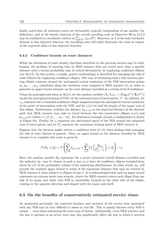
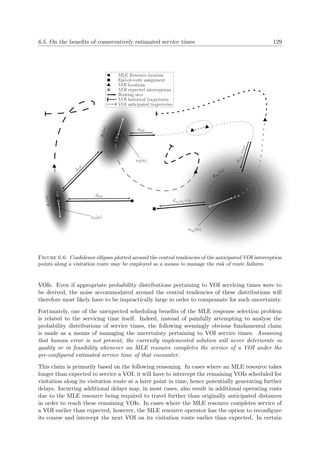
![130 Chapter 6. Management of stochastic information
cases where the operator deems additional delay to be less important than incurring additional
operating costs, the MLE resource always has the option of engaging in a wait-and-see strategy
after completing service earlier than expected. This approach may be considered in cases where
the remaining travel arcs are expected to be cumulatively shorter as a result of waiting on the
spot for some period of time. In closing, it is also acknowledged that the same reasoning may
be applied to MLE resource setup times in cases where these are not deterministic.
6.6 Error management of threat evaluation input data
A proposed alternative to the implementation of Objective IV in §4.2.3 in the mathematical
model formulation of the MLE response selection routing problem in respect of managing the risk
of infeasible encounters is to employ pre-defined threshold parameter values. Such parameters
will ensure that an MLE resource is forbidden to be scheduled to investigate a VOI associated
with a probability above a certain threshold of embodying a certain type of threat. Hence, define
the parameter θkh ∈ [0, 1] to be an (upper bound) threshold associated with MLE resource k
and threat type h. The constraint sets
pihτ − θkh ≤ 1 − ukhτ
and
yikτ ≤ ukhτ , i ∈ Ve
τ , k ∈ Vr
, h ∈ H
may then be incorporated into the model formulation as a means of implementing such an
alternative towards lowering the overall risk of infeasible encounters, where ukhτ ∈ {0, 1} is a
linking constraint variable. In the above constraint set formulation, MLE resource k is only
authorised to intercept VOI i during time stage τ if pihτ ≤ θkh for all h ∈ H. These constraints
are only applicable to strictly incapable assignments; that is, there is no need to incorporate
such constraints in respect of an MLE resource that it is not strictly incapable of handling a
type of threat on its own.
The above approach may reduce the risk of infeasible encounters significantly when strict enough
threshold parameters are established, and is easily implementable in the model formulation.
Defining these threshold parameters in a subjective manner, however, may be a tedious process,
and these parameters will most likely have to be reevaluated in the long run in order to accurately
reflect the preferences of the coastal nation in that regard (for example, due to changes in the
set of MLE resources, changes of operators, changes of threat intensity values and changes of
national policies).
6.7 Dominance assessment in stochastic multiobjective spaces
The focus in this section shifts from considering stochastic elements in the domain space of a
problem instance to its corresponding objective space. In the MLE response selection problem,
two objective functions essentially ought to be defined probabilistically, namely the operating
costs and the total delay times. On the one hand, operating costs mainly consist of the travelling
costs of MLE resources which, as acknowledged in §6.4, may be highly stochastic. On the
other hand, total delay times is even more highly stochastic, as it is itself determined by two
stochastic elements, namely travel times and service times. It is assumed that threat evaluation
systems already accommodate highly central probability distributions (i.e. small uncertainty in](https://image.slidesharecdn.com/6cd1ebf5-5cfe-4d40-998c-99cbe17b08f1-170109122537/85/PhD-dissertation-162-320.jpg)
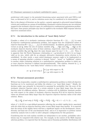
![132 Chapter 6. Management of stochastic information
be most suited to model the stochastic nature of the operating costs and delay times of visita-
tion routes. The following two identities may therefore prove to be useful in this problem: (1) if
Ox ∼ Γ(ax, θ) and Ox ∼ Γ(ay, θ), then (Ox−Oy) ∼ Γ(ax−ay, θ), and (2) if Ox ∼ N(µx, σ2
x)
and Ox ∼ N(µy, σ2
y), then (Ox − Oy) ∼ N(µx − µy, σ2
x + σ2
y). The computations may, how-
ever, become very tedious to carry out if the two random variables are governed by different
probability distributions or if the random variables are defined non-parametrically, particularly
considering that these calculations must be carried out rapidly during the course of a solution
search process.
6.7.3 Alternative assessment procedures
In cases where the probability P(Ox > Oy) is not easily assessed, a subset of the following three
proposed alternative stochastic dominance conditions may, alternatively, be employed:
1. Ox Oy if and only if P(Ox < E[Oy]) < β∗,
2. Ox Oy if and only if P(Oy > E[Ox]) < γ∗, and
3. Ox Oy if and only if 1 −
+∞
−∞ f(ox)f(oy)do < 1 − ζ∗.
In the first condition above, the probability that the objective function value ox is greater than
the central tendency (i.e. the expected value) of the objective function value oy, which must be
larger than a user-defined parameter β∗ ∈ (0, 0.5) for the random variable Ox to be considered
most likely larger than the random variable Oy. The probability P(Ox < E[Oy]) is indicated
graphically in Figure 6.7 by the shaded areas β.
Similarly, the second condition above evaluates the probability that the objective function value
oy is greater than the central tendency of the objective function value ox, which must be
smaller than a user-defined parameter γ∗ ∈ (0, 0.5) for the random variable Ox to be considered
most likely larger than the random variable Oy. The probability P(Oy > E[Ox]) is indicated
graphically in Figure 6.7 by the shaded areas γ.
While these conditional approaches are relatively easily computed, they should, however, not
be implemented on their own. Condition 1 does not take into consideration the magnitude of
the variance of the random variable Oy. As a result, although it may appear as if there ex-
ists a convincing case that Ox is larger than E[Oy], it may also very well be the case that a
large (unacknowledged) probability γ is present, in turn indicating that there exists a significant
counter-possibility that Oy is larger than E[Ox]. A similar reasoning is applicable to Condi-
tion 2. It is thus recommended that Conditions 1 and 2 be employed simultaneously rather than
on their own, noting, however, that such a union requires two user-defined parameters.
Lastly, although much more challenging to compute, one may also consider the so-called modified
Hellinger distance [98] underpinned by Condition 3 above. This metric is defined on the interval
(0, 1) and agrees with the triangle inequality. Moreover, it is indicative enough to be employed on
its own and only requires one user-defined parameter (namely ζ∗). A drawback of implementing
this measure, however, arises from the possibly high level of complexity involved in assessing the
product of the two underlying probability distributions. From a visual point of view, the (non-
modified) Hellinger distance of two probability distributions sharing the same domain space is,
in most cases, reflected by the surface area (in the univariate case) of the overlapping region
between these two distributions [96].](https://image.slidesharecdn.com/6cd1ebf5-5cfe-4d40-998c-99cbe17b08f1-170109122537/85/PhD-dissertation-164-320.jpg)
![6.7. Dominance assessment in stochastic multiobjective spaces 133
fN
∗x(o
∗
x)fN
∗y(o
∗
y)
E[O
∗
y ] E[O
∗
x ]
β γ
(a) Objective function mappings governed by Gaussian probability dis-
tributions.
fΓ
∗x(o
∗
x)
fΓ
∗y(o
∗
y)
E[O
∗
y ] E[O
∗
x ]
β
γ
(b) Objective function mappings governed by Gamma probability dis-
tributions.
Figure 6.7: Mappings of two decision vectors x and y by stochastic objective function ∗
according to
two types of probability distributions fN
and fΓ
.
6.7.4 A numerical example
To illustrate the workings of the stochastic dominance measures proposed above, a basic nu-
merical example is provided in this section9. Suppose that the operating costs Ocosts
x (noting
that this objective is to be minimised on the domain R+) associated with solution x may be
modelled probabilistically by a Gaussian distribution with mean $3 500 and standard deviation
$90, and suppose that the operating costs Ocosts
y associated with solution y may be modelled
probabilistically by a Gaussian distribution with mean $3 700 and standard deviation $125.
That is, let Ocosts
x ∼ N(3 500, 8 100) and Ocosts
y ∼ N(3 700, 15 625).
The formal assessment procedure of §6.7.2 is first considered. It follows directly from the ob-
servations made in §6.4 for the random variable Z = Ocosts
y − Ocosts
x that Z ∼ N(200, 23 725).
Using the software package MATLAB [147],
P(Ocosts
x < Ocosts
y ) = P(Z > 0) =
∞
0
fN (z)dz = 0.903.
By definition, Ocosts
x Ocosts
y provided that the rigidity factor satisfies η∗ > 0.097. The domi-
9
For the sake of clarity, some of the symbols in this example are simplified from their formal definitions.](https://image.slidesharecdn.com/6cd1ebf5-5cfe-4d40-998c-99cbe17b08f1-170109122537/85/PhD-dissertation-165-320.jpg)
![134 Chapter 6. Management of stochastic information
nance measure pertaining to Condition 1 in §6.7.3 is given by
P(Ocosts
x > E[Ocosts
y ]) =
∞
3 700
fN (ocosts
x )docosts ≈ 0.013,
while the dominance measure pertaining to Condition 2 in §6.7.3 is given by
P(Ocosts
y < E[Ocosts
x ]) =
3500
−∞
fN (ocosts
y )docosts ≈ 0.045.
Finally, the modified Hellinger distance of §6.7.3 is assessed. According to Bromiley [15], the
distribution of the product of two independent Gaussian random variables is given by
fNx(o)fNy(o) =
ψxy
2π
σ2
xσ2
y
σ2
x+σ2
y
exp
−
w −
µxσ2
y+µyσ2
x
σ2
x+σ2
y
2
2
σ2
xσ2
y
σ2
x+σ2
y
,
which is clearly governed by a scaled Gaussian probability density function, where
ψxy =
1
2π(σ2
x + σ2
y)
exp −
(µx − µy)2
2(σ2
x + σ2
y)
is itself a Gaussian probability density function modelling the random variable µx − µy with
mean 0 and standard deviation σ2
x + σ2
y. Letting fNx(o)fNy(o) = fW (w), the density func-
tion may be written as
fW (w) ≈
e− 4 000
47 450
√
2π
√
5 335
√
2π
√
23 725
exp −
(w − 3 568)2
2(5 335)
≈
0.919
√
2π 28 200
exp −
(w − 3 568)2
2(5 335)
≈
1
√
2π 30 685
exp −
(w − 3 568)2
2(5 335)
≈ 0.00238
1
√
2π
√
5 335
exp −
(w − 3 568)2
2(5 335)
,
so that W ∼ 0.00238 (N(3 568, 5 335)). Next, it is required to assess the density function of
the random variable V =
√
W. Before going any further, noting that V, W ∈ [0, ∞) and that
the mapping of this function is both bijective and monotonically increasing, it is anticipated
that FV (∞) = 0.00238(FW (∞)) = 0.00238. For the sakes of interest and validation, however,
observe that FV (v) = P(V ≤ v) = P(
√
W ≤ v) = P(W ≤ v2) = FW (v2). Applying the chain
rule for differentiation, the density function fV (v) may be formulated as
fV (v) =
d
dv
FV (v) = fW (v2
)
d
dv
v2
= 2vfW (v2
).
Using the software package MATLAB [147], it follows that
∞
0
fV (v) dv =
0.00238
√
2π
√
5 335
∞
0
2v exp −
(v2 − 3 568)2
10 670
dv
≈
0.00238
√
2π
√
5 335
(183.0868)
≈ 0.00238,](https://image.slidesharecdn.com/6cd1ebf5-5cfe-4d40-998c-99cbe17b08f1-170109122537/85/PhD-dissertation-166-320.jpg)


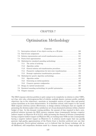
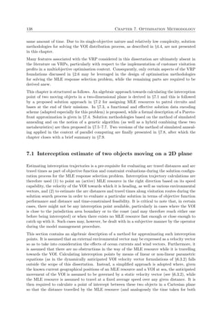
![7.1. Interception estimate of two objects moving on a 2D plane 139
objects to reach that point) is minimised. This problem can be solved in constant time (i.e. no
iterative steps are necessary).
As described in the previous chapter, the oceanic open plane staging the MLE response selection
operations of a coastal nation may be expressed as a bounded two-dimensional space with global
basis {bx, by}. Under the above-mentioned assumptions, let the position of the VOI at time t = 0
be denoted by P κ = [xκ yκ] and let its velocity vector be denoted by vκ = [sκx sκy], where sκx is
the velocity component of the VOI in the direction of the basis vector bx and sκy is the velocity
component of the VOI in the direction of the basis vector by. Furthermore, let η be the average
achievable speed of the scheduled MLE resource (which is assumed to be fixed over any distance),
let P ω = [xω yω] be the position of the MLE resource at time t = 0 and denote the (unknown)
velocity vector of the MLE resource by vω = [sωx sωy], where sωx is the velocity component of
the MLE resource in the direction of the basis vector bx and sωy is the velocity component of
the MLE resource in the direction of the basis vector by. Moreover, define the environmental
velocity vector vζ = [sζx sζy] to embody all outside forces impacting the motion of objects at sea,
such as current vectors and/or wind vectors. Finally, let the (unknown) coordinates P = [x y ]
represent the expected point of interception in space of these two objects and let t ≥ 0 be the
time at which these two objects are expected to reach each other. These vector components are
presented graphically in Figure 7.1.
Γ
sωy
sωx
sζy
sζx
sκy
sκx
sζy
−sζx
Pω
Pκ
P
MLE resource
VOI
Interception point
Figure 7.1: Computing the point of interception for two objects at sea.
In order to solve this interception problem, it is only necessary to solve for the unknowns sωx,
sωy and t . The interception coordinates of P are then given by
x = xκ + (sκx + sζx) t and y = yκ + (sκy + sζy) t . (7.1)
Additionally, the interaction between the norm of the velocity vector of the VOI and the speed
of the resource at the point of intersection, with respect to time, may be described as
||P κ + (vκ + vζ) t 2 = P ω + (vω + vζ) t 2, (7.2)
where || · ||2 denotes the well-known L2-norm. Applying the definition of the L2-norm in a
Cartesian plane, (7.2) may be rewritten as
(xκ + (sκx + sζx) t )2
+ (yκ + (sκy + sζy) t )2
= (xω + (sωx + sζx) t )2
+ (yω + (sωy + sζy t )2
. (7.3)](https://image.slidesharecdn.com/6cd1ebf5-5cfe-4d40-998c-99cbe17b08f1-170109122537/85/PhD-dissertation-171-320.jpg)
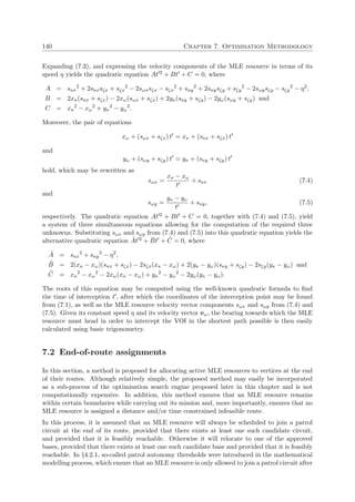
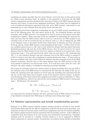

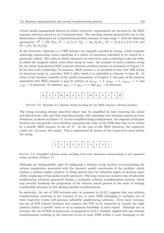
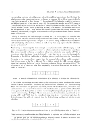

![146 Chapter 7. Optimisation Methodology
Fully formed solution
Refine the
solution string with
trip delimiters
Remove necessary model
management VOIs
from the string
Perform general sub-
transformation on
the reduced string
Perform reinsertion
sub-transformation
Perform end-of-route
assignment sub-
transformation
Figure 7.8: Flow of events in the proposed overall solution transformation procedure.
the computational resources available for solving the problem, such as the search time, processing
power or storage capacity, are tightly constrained). Moreover, finding a good approximation of
even a portion of the Pareto front is difficult when the structure of the underlying domain space
is not known or is very disjoint [44].
According to Zitzler et al. [167], a multiobjective search technique should always aim to achieve
three conflicting goals with respect to the nature of the resulting non-dominated front. First,
the non-dominated front should ideally be as close as possible to the true Pareto front. The non-
dominated set of solutions should, in fact, preferably be a subset of the true Pareto-optimal set
if possible. Secondly, solutions in the non-dominated set should ideally be uniformly distributed
and diverse with respect to their objective function values along the Pareto front so as to provide
the decision maker with the full picture of trade-off decisions. Lastly, the non-dominated front
should ideally capture the entire range of values along the true Pareto front.
Here, the first goal is best served by focusing the search on a particular region of the true Pareto
front — a process known in the literature as intensification (or exploitation). On the other
hand, the second goal requires the search technique to investigate solutions that are uniformly
distributed along the true Pareto front — a process known in the literature as diversification
(or exploration). Finally, the third goal aims to extend the non-dominated front at both ends
of the true Pareto front in order to explore new, extreme solutions.
In the next two sections, two familiar solution search methodologies which may be incorpo-
rated into the optimisation methodology component of the MLE response selection DSS of this
dissertation are presented, namely the archived multiobjective simulated annealing algorithm
(mentioned in §2.3.3) and the NSGA-II (mentioned in §2.4.2). These solution search techniques
have been documented extensively in the literature as being capable of achieving the above three
goals for a wide variety of problems, provided that their algorithmic configurations (parameter
values) are chosen carefully. Furthermore, a hybrid approach combining these two algorithms
and two multi-start simulated annealing algorithms adapted from the (single-start) algorithm
in [131] are also developed.
7.5 Multiobjective simulated annealing methodology
In §2.3.3, a brief review of key multiobjective simulated annealing techniques from the literature
was conducted and it was mentioned in §2.6.5 that certain of these techniques may be adapted
for solving multiobjective VRPs when tuned appropriately (in terms of parameter value choices).](https://image.slidesharecdn.com/6cd1ebf5-5cfe-4d40-998c-99cbe17b08f1-170109122537/85/PhD-dissertation-178-320.jpg)
![7.5. Multiobjective simulated annealing methodology 147
In this section, the innovative multiobjective simulated annealing algorithm proposed for this
purpose by Smith et al. [130, 131] is described in some detail, following which certain simulated
annealing solution transformation methods which comply with the unique nature of the MLE
response selection problem are proposed.
7.5.1 The notion of archiving
Because the method of simulated annealing only generates a single solution during each iteration
of the search process, an external set, known as the archive, is employed to record all non-
dominated solutions uncovered during the course of the search process. All solutions generated
during the course of the search are candidates for archiving, and are each tested for dominance
in respect of every solution in the archive. The archiving process is illustrated in Figure 7.9 for
a bi-objective minimisation problem with objective functions f1 and f2.
f1
f2
Solutions not archived
Existing solutions in the archive
New solution added to the archive
Archived solution removed
Figure 7.9: The archiving process for a bi-objective minimisation problem.
If the true Pareto front P were available a priori, it would be possible to express the energy
(i.e. the performance of a solution in objective space) of a solution x as some measure of the
portion of the front that dominates x. To this effect, let Px be the portion of P that dominates
x (i.e. Px = {y ∈ P | y x}), and define the energy of x as E(x) = M(Px), where M is a
measurable function defined on P. If P is continuous, M may be configured as the Lebesgue
measure; otherwise M may simply be configured as the cardinality of Px (i.e. the number of
solutions in P that dominate x). Of course, E(x) = 0 for all x ∈ P.
As the true Pareto front is typically unavailable during the course of the search, however, the
energy of a solution is instead measured based on the current estimate of the true Pareto
front, which corresponds to the set of non-dominated solutions uncovered thus far during the
search (that is, the solutions in the archive). The energy difference between two solutions is
measured as the quotient of the difference in their respective energies and the size of the archive.
According to Smith et al. [131], a simulated annealer that uses this energy measure encourages
both convergence to and coverage of the Pareto front in logarithmic computational time.](https://image.slidesharecdn.com/6cd1ebf5-5cfe-4d40-998c-99cbe17b08f1-170109122537/85/PhD-dissertation-179-320.jpg)
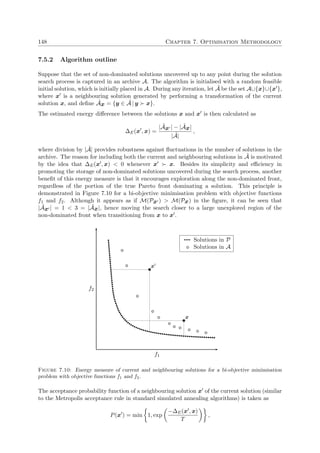
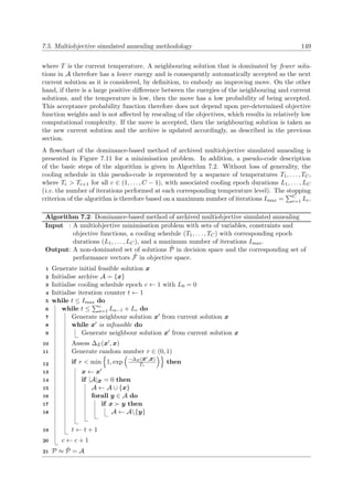
![150 Chapter 7. Optimisation Methodology
Generate initial solution x
Create archive A
Set initial temperature
Generate neighbour
solution x
∆E(x , x)
≤ 0 ?
Accept move
True
Accept move
with probabil-
ity e{
−∆E(x ,x)
Tc
}
False
Move
accepted?
False
True
Set x = x
x dominated
in A?
Add x to
the archive
FalseTrue
Remove solutions dominated
by x from the archive
Epoch
completion?
False
True
t > Imax ?
Report
non-dominated set
True
Lower temperature
according to
cooling schedule
False
Figure 7.11: Flow of events in the dominance-based, archived multiobjective simulated annealing algo-
rithm of Smith et al. [131].](https://image.slidesharecdn.com/6cd1ebf5-5cfe-4d40-998c-99cbe17b08f1-170109122537/85/PhD-dissertation-182-320.jpg)
![7.5. Multiobjective simulated annealing methodology 151
7.5.3 General solution sub-transformation procedures
Two general types of solution transformation methods are typically employed in the simulated
annealing literature for generating neighbouring solutions in a VRP, namely intra-route transfor-
mations and inter-route transformations [156]. An intra-route transformation technique changes
a route within the same solution string by altering one or more partial strings within that route
in an attempt to improve it. An inter-route transformation, on the other hand, exchanges
or relocates one or more partial strings between any routes of a VRP solution string. These
transformations are used to encourage exploitation and diversification of the search, respectively.
Researchers are often required to improvise their own solution transformation techniques in
order to better accommodate certain types of VRPs and/or try to improve the search process in
general. In [156], for example, three inter-route improvement methods are proposed. These are
the string exchange method, where two partial strings from two different routes are exchanged
with one another at specific locations within the routes, the string relocation method, where a
partial string containing one or more entries from one route is inserted into a specific location
within another route, and the string mix method, which attempts to relocate or exchange partial
strings.
More generic methods of transformation are the one-to-one exchange, delete-and-insert and
partial string reversal [80, 140, 156], which are applicable to both intra-route and inter-route
transformations. These techniques also allow for the zero delimiters in a string to be moved
around, so as to change the nature and size of the routes pre-assigned to the vehicles. The
first two methods are similar to the string exchange and string relocation methods, respectively,
as described in the previous paragraph. The partial reversal method consists of temporarily
removing part of the string, reversing the direction of that partial string, and either placing it
back where it was originally removed or inserting it somewhere else in the string.
In addition, however, the VRP customer visitation profits characteristic associated with the MLE
response selection problem requires transformations that alter the number of VOIs scheduled
to be intercepted by adding or removing partial strings to or from the current solution. Such
transformations are defined in this dissertation as inter-state transformations, where the state
of a solution is defined as the number of VOIs visited in a solution. More specifically, a string
expansion transformation is defined as one that increases the number of VOIs in the current
solution string by inserting one or more partial strings containing currently unvisited VOIs
stored from an external set into it. A string diminution transformation is similarly defined as
one that decreases the number of VOIs in the current solution string by removing one or more
partial strings from it.
Examples of some of the above solution transformation procedures for VRP solution strings are
illustrated in Figure 7.12. For the sake of clarity, note from §7.3 that these actually constitute
general sub-transformation procedures. Here, Figures 7.12 (a) and (b) represent intra-route
transformations, while Figures 7.12 (c) and (d) represent inter-route transformations. Figures
7.12 (e) and (f) finally represent inter-state transformations.
At every iteration, it is therefore proposed that a type of solution transformation move be selected
according to a pre-configured probability distribution, where the parameter PWR ∈ [0, 1] is the
probability of conducting an intra-route transformation, while the parameter PBR ∈ [0, 1] is
the probability of conducting an inter-route transformation and the parameter PS ∈ [0, 1] is
the probability of conducting an inter-state transformation. Of course, PWR + PBR + PS =
1. In addition, there may be several sub-types of moves within each of these transformation
classes, which are also triggered according to a certain probability distribution. For example,
the user may wish to conduct a delete-and-insert or a partial reversal move according to certain](https://image.slidesharecdn.com/6cd1ebf5-5cfe-4d40-998c-99cbe17b08f1-170109122537/85/PhD-dissertation-183-320.jpg)
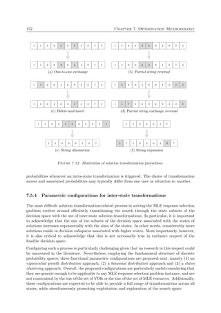
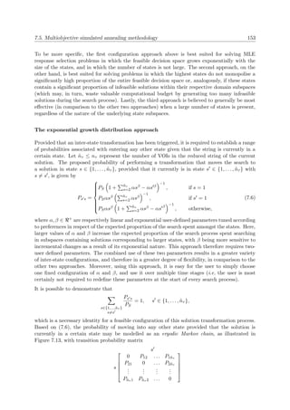
![154 Chapter 7. Optimisation Methodology
and steady-state probabilities
1
1 + ˜nτ
s=2 αsβ
α(2β)
1 + ˜nτ
s=2 αsβ
. . .
α(˜nβ
τ )
1 + ˜nτ
s=2 αsβ
.
According to the law of large numbers [52], the expected proportion of the search spent in each
state therefore approaches that of the entries in the vector above as the number of algorithmic
iterations approaches infinity. Again, it is possible to demonstrate that the sum of these entries
add up to 1. These steady-state probabilities may, however, not accurately reflect the desired
search repartition if the number of iterations performed by the algorithm is too small and the
number of states is too large.
1 2
P21
P12
. . . . . . . . . . . . . . . . . . . . . . . . . . . . . . ˜nτ
P˜nτ 1
P1˜nτ
P˜nτ 2
P2˜nτ
Figure 7.13: Markov chain of inter-state transition probabilities.
The binomial distribution approach
A random variable U ∼ (˜n, p) is governed by a binomial probability distribution based on ˜n trials
with success probability p if
P(U = u) =
˜n!
u!(˜n − u)!
pu
(1 − p)˜n−u
, u ∈ {0, 1, . . . , ˜n}.
Here, the distribution parameter ˜n once again represents the maximum number of VOIs that
may be visited in a reduced solution string, while the user-defined parameter p is responsible for
steering the expected proportion of the search spent in every state. This approach therefore only
requires one user-defined parameter, where the search process is expected to spend more time
investigating higher-state solutions whenever a higher success probability parameter is employed.
Furthermore, the probability of performing a transformation that moves the search to a solution
in state u ∈ {0, 1, . . . , ˜n}, provided that it currently is in state u ∈ {0, 1, . . . , ˜n} with u = u , is
given by
Pu u = PS
P(U = u)
1 − P(U = u )
,
where
u∈{0,1,...,˜n}
u=u
Pu u
PS
= 1, u ∈ {0, 1, . . . , ˜n}.
Because state 0 contains only one solution, which may easily be evaluated a priori, it is noted
that it would be impractical to allocate a computational budget to access this state. If P(U = 0)
is very small, this issue is trivial. If this probability is not insignificant, however (such as in](https://image.slidesharecdn.com/6cd1ebf5-5cfe-4d40-998c-99cbe17b08f1-170109122537/85/PhD-dissertation-186-320.jpg)
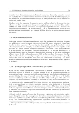
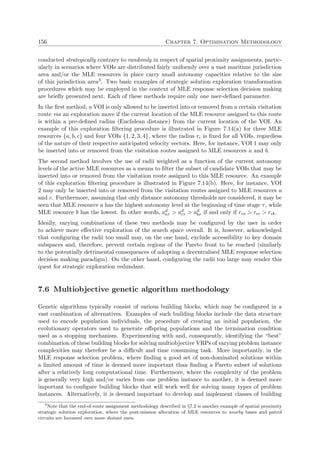
![7.6. Multiobjective genetic algorithm methodology 157
1
2
3
4
a
b
c
r
(a) Visitation route candidate allocations with fixed
VOI radii.
1
2
3
4
a
ra
b
r b
c
r c
(b) Visitation route candidate allocations
with weighted MLE resource radii.
Figure 7.14: Illustrations of strategic exploration transformation procedures with respect to spatial
proximity assignments.
blocks into the DSS that may be used for specific classes of problem instances, rather than
having to identify the best combination of building blocks at the start of a problem instance
prior to launching the solution search process.
In §2.4.2, a review was presented of key multiobjective genetic algorithm techniques from the
literature and it was mentioned in §2.6.5 that certain of these techniques may be used to solve
complex multiobjective VRPs. In this section, the working of the non-dominated sorting genetic
algorithm II (NSGA-II), proposed by Deb et al. [41], is described in some detail and ideas are
proposed for generating an initial population and designing unique genetic operators adapted
to accommodate the nature of the MLE response selection problem.
7.6.1 Algorithm outline
In this population-based NSGA-II, an initial population of candidate solutions of size N is first
randomly generated. These solutions are then ranked and sorted into sets, called non-dominated
fronts, using the so-called Fast Non-dominated Sorting Algorithm (FNSA) [41] as a means of
assessing the fitness levels of individuals4. The FNSA works as follows. For each individual p, the
domination count nc
p is defined as the number of solutions in the population dominating p, while
Dp is defined as the set of solutions dominated by p. All solutions with a dominance count value
nc
p = 0 are then placed in a set F1 called the first non-dominated front. Next, for each solution
p ∈ F1, each individual q ∈ Dp is visited and its domination count nc
q is reduced by one, thus
disregarding the dominance effect of solution p on solution q. The solutions with an updated
dominance count of 0 are then placed in the second non-dominated front, F2. The same process
is repeated to identify members of a third non-dominated front, and so forth, until all individuals
have been placed in some non-dominated front. An example illustrating the notion of domination
fronts for a bi-objective minimisation problem with N = 11 and objective functions f1 and f2
4
The terms “individuals” and “solutions” are used interchangeably throughout this section.](https://image.slidesharecdn.com/6cd1ebf5-5cfe-4d40-998c-99cbe17b08f1-170109122537/85/PhD-dissertation-189-320.jpg)
![158 Chapter 7. Optimisation Methodology
is shown in Figure 7.15. The non-domination rank prank ∈ N of individual p is then simply
defined as the cardinal number of its non-dominated front. A pseudo-code description of this
non-dominated sorting approach is presented in Algorithm 7.3. The worst-case computational
complexity of this sub-process is O(MN2), where M is the number of objective functions. In
contrast, the complexity of the non-dominated sorting mechanism used in the original NSGA-I
is O(MN3) [134].
f1
f2
Solutions in F1
Solutions in F2
Solutions in F3
Figure 7.15: Illustration of domination fronts in the NSGA-II for a bi-objective minimisation problem.
Relatively fast convergence to the Pareto-optimal set (i.e. elitism preservation) is one benefit of
employing the FNSA described above. However, it is also required to maintain a good spread of
solutions within the search space at every generation (i.e. maintain diversity preservation), as
described in §7.4. In order to achieve this, the algorithm incorporates a simple procedure taking
the density estimation of individuals into consideration (that is, an estimate of the density of
solutions surrounding an individual in a particular non-dominated front in objective space). The
density estimation of an individual pdist, called its crowding distance, is calculated by taking the
average distance of two solutions on either side of that individual along every objective. The so-
lutions are ranked from lowest to highest with respect to each objective function. The boundary
solutions (i.e. the solutions with the highest and lowest objective function scores) are assigned
an infinite crowding distance, while an intermediate solution is assigned a crowding distance
that is measured indirectly proportionally to the proximity of its two neighbours alongside each
objective function.
The purpose of the crowding distance operator is therefore to quantify the density of a solution,
where a lower value suggests that a solution is more “crowded” by other solutions. This approach
does not require the specification of any user-defined parameters for maintaining diversity. A
pseudo-code description of the crowding distance procedure is presented in Algorithm 7.4, where
P (i)|o represents the ith individual in the population ranked with respect to objective o, while
fmax
o and fmin
o are respectively the maximum and minimum values achieved by individuals along
the axis of the oth objective function. The worst-case computational complexity of this procedure
is O(MN log N) [41]. In contrast, the complexity of the diversity conservation mechanism used
in the NSGA-I is O(MN2) [41, 134].
In order to guide the selection process of the algorithm towards a uniformly spread approximately](https://image.slidesharecdn.com/6cd1ebf5-5cfe-4d40-998c-99cbe17b08f1-170109122537/85/PhD-dissertation-190-320.jpg)
![7.6. Multiobjective genetic algorithm methodology 159
Algorithm 7.3: Fast non-dominated sorting algorithm (FNSA) [41]
Input : A population P containing N solution vectors {p1, . . . , pN } in decision space
together with the corresponding vectors in objective space.
Output: The set of non-dominated fronts F1, . . . , FF partitioning the solutions in P .
F1 ← ∅1
forall p ∈ P do2
Dp ← ∅3
nc
p = 04
forall q ∈ P do5
if p q then6
Dp ← Dp ∪ {q}7
else if q p then8
nc
p ← nc
p + 19
if nc
p = 0 then10
prank ← 111
F1 ← F1 ∪ {p}12
← 113
while F = ∅ do14
G ← ∅15
forall p ∈ F do16
forall q ∈ Dp do17
nc
q ← nc
q − 118
if nc
q = 0 then19
qrank ← + 120
G ← G ∪ {q}21
← + 122
F ← G23
Algorithm 7.4: Crowding distance assignment algorithm [41]
Input : A population P of size N containing solution vectors {p1, . . . , pN } and the
corresponding performance vectors in the M-dimensional objective space.
Output: The crowding distance for each solution in P .
forall i ∈ N do1
pdist
i ← 02
forall o = 1, . . . , M do3
P ← sort(P , o)4
pdist
P (1)|o
← ∞5
pdist
P (N)|o
← ∞6
forall i = 2, . . . , N − 1 do7
pdist
i ← pdist
i + (P (i + 1)|o − P (i − 1)|o)/(fmax
o − fmin
o )8](https://image.slidesharecdn.com/6cd1ebf5-5cfe-4d40-998c-99cbe17b08f1-170109122537/85/PhD-dissertation-191-320.jpg)
![160 Chapter 7. Optimisation Methodology
Pareto optimal front, a so-called crowded-comparison operator C is employed. This operator
assesses the rank as well as the crowding distance, as described above, in order to determine
superiority between any two solutions, which is used as the selection operator of the algorithm.
The rank serves as the first assessment criterion, where a solution achieving a lower rank value
is considered superior. If two solutions achieve the same rank value, then the solution achieving
the higher crowding distance is considered superior. Mathematically,
p C q
if prank < qrank
or prank = qrank and pdist > qdist ,
and the computational complexity of sorting on the operator C is O(N log N) [41]. In this
way, the search will favour the exploration of solutions in less crowded regions of the solution
space which, in turn, leads to a more uniformly spaced non-dominated front.
Overall, the NSGA-II works as follows. The algorithm is initialised by randomly creating an
initial parent population P 0 of size N and is iterated until a pre-specified number of generations
is achieved. Generation t begins with an initial parent population P t of size N. The FNSA is
called, and each solution is assigned a fitness level proportional to its rank. The usual genetic
operators, such as tournament selection, crossover and mutation are then applied to create an
offspring population Qt of size N, after which the parent and child individuals are combined to
form a larger intermediate population Rt = P t ∪ Qt of size 2N. This intermediate population
is then sorted and ranked into non-dominated fronts again, after which the next population of
candidate solutions P t+1 is generated by first including the solutions in the first non-dominated
front F1, then the solutions in the second non-dominated front F2, and so on, until a population
of size N is reached. Because all individuals in the last included front most likely cannot all be
selected to add up to the pre-required population size N, they are ranked in descending order
with respect to their crowding distances and the best solutions are chosen one by one until
the desired size N is reached for the new population. An illustration of the operation of the
NSGA II is shown in Figure 7.16, a flowchart of the algorithm is presented in Figure 7.17 and
a pseudo-code description of the algorithm is given in Algorithm 7.5.
7.6.2 Generating an initial population
There is general consensus in the literature that an initial population which is too small has a
higher chance of guiding the search towards poor solutions, while an initial population which is
too large may incur an unrealistically large computational burden in order to find a good set
of non-dominated solutions [24, 79, 169]. According to Diaz-Gomez et al. [45], finding a good
initial population combined with the optimal population size is a difficult problem, and there
exists no general rule for this purpose which can be applied to every type of problem. They
acknowledge that the search space, fitness function, diversity, problem difficulty and selection
pressure are all factors that may and should also be considered in order to create a good initial
population.
The notion of subspecies is introduced to fulfil the role of a state, as described in §7.5.3. A
subspecies is a subpopulation containing all individuals in a specific state. The process of
creating an initial population for the MLE response selection problem primarily evolves around
the distribution of subspecies, which was found, after extensive numerical experimentation, to
have a significant impact on the nature and distribution of subspecies in future generations. A
subspecies is said to become extinct if the number of individuals in this subspecies is reduced
to zero from one generation to the next one. Extinctions are better avoided, particularly during](https://image.slidesharecdn.com/6cd1ebf5-5cfe-4d40-998c-99cbe17b08f1-170109122537/85/PhD-dissertation-192-320.jpg)
![7.6. Multiobjective genetic algorithm methodology 161
Algorithm 7.5: The Non-dominated Sorting Genetic Algorithm II (NSGA-II) [41, 90]
Input : A multiobjective optimisation problem with sets of variables, constraints and
objective functions, the size of the population N and the maximum number of
generations Gmax.
Output: A non-dominated set of solutions ˜P in decision space and the corresponding set of
performance vectors ˜F in objective space.
Generate a random feasible initial population P 0 of size N1
Sort the individuals in P 0 into their respective non-dominated fronts using Algorithm 7.32
and assign them a rank
Assess the crowding distance of each solution in P 0 using Algorithm 7.43
Generate an initial offspring population Q0 of size N using tournament selection; favour4
individuals competing for reproduction first based on their ranks and then on their
crowding distances
t ← 05
while t < Gmax do6
Rt ← P t ∪ Qt7
Sort Rt into non-dominated fronts F1, . . . , FF using Algorithm 7.38
P t+1 ← ∅9
← 110
while |P t+1| < N do11
if |P t+1| + |F | ≤ N then12
P t+1 ← P t+1 ∪ F13
else if |P t+1| + |F | > N then14
Assess the crowding distance of each solution in F similarly to Algorithm 7.415
F = sort(F , C)16
c ← 117
while |P t+1| + c ≤ N do18
P t+1 ← P t+1 ∪ F (c)19
c ← c + 120
← + 121
Assess the crowding distance of each solution in P t+122
Generate an offspring population Qt+123
t ← t + 124
P ≈ ˜P = F125](https://image.slidesharecdn.com/6cd1ebf5-5cfe-4d40-998c-99cbe17b08f1-170109122537/85/PhD-dissertation-193-320.jpg)
![162 Chapter 7. Optimisation Methodology
Pt
Qt
F1
F2
F3
F4
...
FF
Pt+1
Non-dominated
sorting
Crowding distance
sorting
Figure 7.16: Sequence of operations carried out in the NSGA-II.
early stages of the evolution process, as they may significantly affect the diversity status of the
final population and promote premature convergence.
The proposed crossover operator (presented later in this section) allows for inter-subspecies
reproduction, but does not allow for offspring solutions from different subspecies to that of
their parents to be generated. Indeed, not only does this idea go strongly against nature, but
may also create offspring solutions that differ too much from their parents, hence defeating the
purpose of passing on strong genetic material from the parent population through inheritance.
Three incentives are employed in an attempt to reduce the extent of the problem of extinction:
(1) a large initial population is generated with subspecies that are assigned large enough sizes;
(2) an immigration operator is introduced in which the immigrants are individuals which belong
to subspecies that have become extinct or are dangerously close to becoming so; and (3) the
mutation operator is configured to apply inter-state transformations.
In respect of solution transformations using genetic operators, individuals are represented by
means of chromosome strings composed of cells, as described in §7.3. If the size of the initial
population is deemed too small or if the subspecies vary too much in size from one another,
then the mutation operator in the proposed genetic algorithm methodology is configured to use
inter-state transformations (see §7.5.3) to mutate solutions according to a certain probability
in order to promote diversity throughout the evolution process, thereby addressing the problem
of extinction described above. Else, a simple intra-route transformation is configured for the
purpose of mutation. Furthermore, it is customary to use tournament selection for developing
the mating pool when applying the NSGA-II [41, 126], where a certain number of individuals
are selected stochastically from the current population, and the fittest ones (assessed using the
crowded comparison operator, as described in the previous section) are paired for reproduction.](https://image.slidesharecdn.com/6cd1ebf5-5cfe-4d40-998c-99cbe17b08f1-170109122537/85/PhD-dissertation-194-320.jpg)
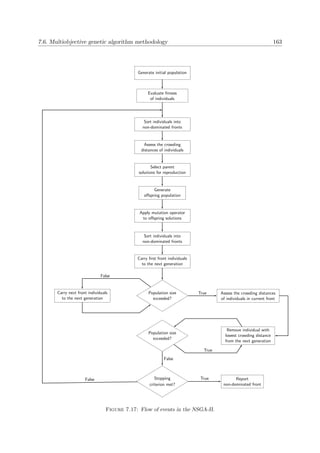
![164 Chapter 7. Optimisation Methodology
7.6.3 Crossover operator configuration
The main property rendering genetic solution representations convenient is that their parts are
easily aligned due to their fixed size which, in turn, facilitates simple crossover operations [81].
Variable solution length representations may also be used, but crossover implementation is more
complex in this case. Moreover, according to Nazif and Lee [106], it may often be necessary
with genetic algorithms not to generate the entire offspring population by means of crossover
operations. In their paper, for instance, they implement a crossover probability of 0.75 for
every pair of parents and a swap operator (i.e. one-to-one exchange) otherwise. In [119], eight
different crossover operators obtained from various previous publications are analysed in respect
of transforming solution strings for VRPs, none of which deal with variable chromosome string
lengths that are applicable to VRPs with customer profits, and this is the same in other, related
publications. Consequently, due to the lack of adequate crossover operators in the literature, a
functional crossover procedure for successfully creating feasible offspring solutions is proposed
in this section for solving the MLE response selection problem by means of the NSGA-II.
Given two selected parent solutions p1 and p2, let Rp1
= {r1(p1), . . . , r|Vr|(p1)}, where rk(p1)
represents the number of VOIs in route k ∈ Vr of the reduced string of parent solution p1.
Similarly, let Rp2
= {r1(p2), . . . , r|Vr|(p2)}. The proposed crossover procedure consists of two
sub-processes, where the second sub-process is only initiated if the first crossover sub-process
fails (with respect to feasibility) after a certain number of mating attempts.
The first crossover sub-process may be described as an adapted version of the traditional cut-
and-splice crossover operator (as described in §2.4.4), which attempts to swap genetic material
from both parents as follows. First, the delimiter cells are removed from their reduced solu-
tion strings to create two chromosome strings containing VOI cells only. A marker function
fM : (|p1|, |p2|) → [1, min{|p1|, |p2|}] is specified by the user, where |p1| refers to the number of
cells in the chromosome string of p1 and |p2| to the number of cells in the chromosome string of
p2. This user-defined step-function generates an integer, called the marker and denoted by M,
in the specified range. The nature of the marker depends on the size of the parent strings, |p1|
and |p2|, as well as on their difference in size. Two offspring solutions o1 and o2 are constructed
by swapping partial strings from the parents (similarly to a cut-and-splice crossover operator),
where the cut is defined by the marker M. A test is then carried out to ascertain whether any of
the two offspring solutions contain duplicate cells in their chromosomes. If one or both of them
do, then the marker value is reduced by one, and the cut-and-splice crossover process is repeated
for p1 and p2, using the updated marker value. This crossover sub-process is terminated when
two offspring chromosomes are formed which do not contain duplicate entries. Converting the
offspring chromosome strings back into a solution format is achieved by configuring Ro1 = Rp2
and Ro2 = Rp1
. These offspring solutions are then tested further for overall feasibility. If
the marker value reaches zero, however, or if one or two of the offspring solutions is classified
as infeasible with respect to overall feasibility (which includes the reinsertion and end-of-route
assignment sub-transformations performed on these reduced offspring solution strings), then the
first sub-process of this crossover procedure is aborted, and the second sub-process is initiated.
An illustrative description of a successful procedure conducted during the first sub-process of
this crossover operator is presented in Figure 7.18. Here, |p1| = 7 and Rp1
= {2, 3, 2}, while
|p2| = 5 and Rp2
= {1, 2, 2}. For demonstration purposes, assume that the original marker
value was specified as M = 3. Then, performing a cut-and-splice crossover procedure on the
two parent chromosomes using this marker clearly results in an infeasible offspring chromosome
(with respect to testing for duplicate entries), as the cell containing entry 5 is duplicated in the
chromosome of the second offspring. However, as depicted in this example, lowering the marker](https://image.slidesharecdn.com/6cd1ebf5-5cfe-4d40-998c-99cbe17b08f1-170109122537/85/PhD-dissertation-196-320.jpg)
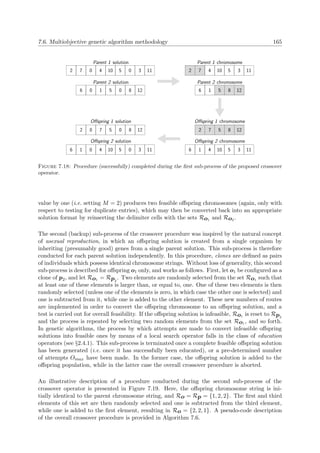
![166 Chapter 7. Optimisation Methodology
Algorithm 7.6: Crossover procedure outline
Input : Two parent solutions p1, p2 with respective route sizes Rp1
and Rp2
, a marker
function fM , and a maximum number of offspring generation attempts Omax.
Output: Possibly feasible offspring solutions o1 and o2.
M ← fM (|p1|, |p2|)1
p1 ← [p11 p12] with [p11] = [p1(1), . . . , p1(M)] and [p12] = [p1(M + 1), . . . , p1(|p1|)]2
p2 ← [p21 p22] with [p21] = [p2(1), . . . , p2(M)] and [p22] = [p2(M + 1), . . . , p2(|p2|)]3
o1 ← [p11 p22]4
o2 ← [p21 p12]5
if either o1 or o2 contain duplicates then6
M ← M − 17
if M ≥ 0 then8
Go to step 29
else10
o ← o111
p ← p212
t ← 113
while (t ≤ Omax) and (o is infeasible) do14
Ro ← Rp15
Generate random numbers r1, r2 such that either Ro(r1) ≥ 1 or Ro(r2) ≥ 116
if r1 ≥ 1 then17
Ro(r1) ← Ro(r1) − 118
Ro(r2) ← Ro(r2) + 119
t ← t + 120
else21
Ro(r1) ← Ro(r1) + 122
Ro(r2) ← Ro(r2) − 123
t ← t + 124
if o is feasible then25
Append o to the offspring population26
if The education operator has been carried onto both offspring solutions then27
STOP28
else29
o ← o230
p ← p131
Go to step 1332
else33
Go to step 1134](https://image.slidesharecdn.com/6cd1ebf5-5cfe-4d40-998c-99cbe17b08f1-170109122537/85/PhD-dissertation-198-320.jpg)
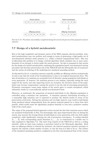

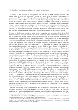
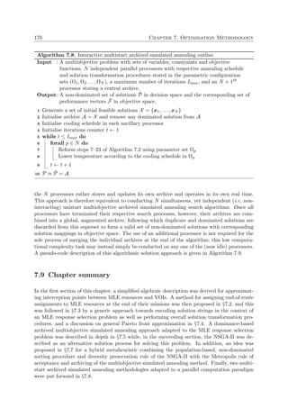


![174 Chapter 8. System Validation
In order to validate the MLE response selection DSS proposed in Chapter 3 and its incorporation
into the MLE system architecture of the same chapter, the aim in this chapter is to gain a better
practical understanding of the mathematical modelling and solution search subsystems by testing
these in the context of two hypothetical MLE response selection scenarios. More specifically, the
modelling of the problem instance embodied in these scenarios is achieved by utilising a subset
of the features described in Chapters 4 and 5, while solving the problem instance is achieved by
applying the optimisation methodologies proposed in Chapter 7.
This chapter is structured as follows. A method for assessing the performance of stochastic
optimisation techniques is first described in 8.1, with particular focus on the well-known hyper-
volume measure, after which an evaluation involving the domain size of any given MLE response
selection problem instance is pursued in §8.2. A lower-complexity hypothetical scenario is then
designed in §8.3 within an intermediate decision making MLE response selection paradigm, and
this is followed §8.4 by a presentation of numerical results which were obtained by solving the
hypothetical problem instance of §8.3 using an array of optimisation techniques. These results
are then analysed and interpreted in some detail. In order to test the optimisation methodology
component under more strenuous conditions, a subset of these experiments is repeated in the
context of a higher-complexity hypothetical scenario in §8.5. Furthermore, recall from Chapter 3
that the proposed DSS also incorporates a post-optimisation solution analysis component, which
has not been discussed so far in the dissertation; its purpose is explained in §8.6. The chapter
finally closes with a brief summary in §8.7.
8.1 Stochastic multiobjective optimisers performance assessment
The comparison of various optimisation techniques by means of experimentation typically in-
volves the notion of performance which, according to Fonseca et al. [58], includes both the quality
of the incumbent solution or non-dominated front, and the time taken to obtain it. The difficulty
in assessing the performance of stochastic optimisation techniques lies in this connection between
solution quality and computation time, which may be reflected by a corresponding probability
density function. In addition, every statement about the performance of such techniques is also
probabilistic in nature.
As discussed in §7.4, the performance of a search technique in the case of multiobjective opti-
misation problems is typically assessed by considering the distance between the non-dominated
front generated and the true Pareto front (which ought to be minimised), the uniformity of the
distribution of the non-dominated solutions in objective space (assessment of this criterion is
usually based on a certain distance metric) and the extent of the non-dominated front across each
objective function (which ought to be maximised). Accurately assessing the respective quality
of non-dominated fronts generated by various multiobjective stochastic optimisation techniques
within specific time frames, while considering the objective function trade-off values and pref-
erences of the decision maker is not a trivial task, particularly in cases where more than two
objective functions are considered [58]. Sound inferences may, however, be made using various
forms of quantitative and statistical information obtained from a series of carefully designed
experiments in order to carry out such assessments.
Two fundamental approaches for evaluating the performance of multiobjective optimisation
techniques are available in the literature, namely the attainment function approach and the
indicator approach [58]. The first approach consists of modelling the outcome of a solution
search process, or run, as a probability density function in objective space, while the second](https://image.slidesharecdn.com/6cd1ebf5-5cfe-4d40-998c-99cbe17b08f1-170109122537/85/PhD-dissertation-206-320.jpg)
![8.1. Stochastic multiobjective optimisers performance assessment 175
summarises the outcome of such a run on the basis of certain quantitative performance measures
by conducting a statistical analysis on the distribution of the performance values. Informally
speaking, the latter approach is typically used for measuring the total portion of the objective
space covered in some sense by the non-dominated front.
If the latter approach is employed, care must be taken when selecting the quality indicator mea-
sure, as every indicator possesses a different underlying structure and, consequently, embodies
certain assumptions about the decision maker’s preferences [58]. It follows that, in any compar-
ative study in which one or more quality indicators are utilised, one may not merely state that
a certain optimiser outperforms another one without acknowledging that such a statement may
only be claimed under the assumption that the utilised indicator(s) fundamentally reflect the
decision maker’s preferences.
8.1.1 The hypervolume quality indicator
The hypervolume indicator, denoted here by Hvol and also known as the S-metric, is a popular
indicator measure used for evaluating the performance of non-dominated fronts. Such an indi-
cator belongs to the class of unary quality indicators, which may be defined as mappings from a
non-dominated set of solutions to the set of positive real numbers. Its purpose is to calculate the
portion of objective space that is collectively dominated by the solutions in the non-dominated
front with respect to a specific, pre-defined vector in objective space, known as the reference
point and chosen in such a way that the non-dominated objective space is bounded by such a
point. The hypervolume measure is usually maximised, and attains its maximum if and only if
the non-dominated front is equal to the true Pareto front.
Informal description and benefits
Consider the set of non-dominated points Sx = {x1, . . . , xN } in the solution space of a multi-
objective optimisation problem with respective performance vectors Sz = {z1, . . . , zN } in ob-
jective space. The hypervolume measure of Sx is then defined as the region dominated by Sz
in objective space from a reference point ¯z satisfying z ¯z for all ∈ {1, . . . , N}. An illus-
tration of the hypervolume measure for a bi-objective minimisation problem using the above
information is shown in Figure 8.1.
The hypervolume indicator is often favoured as a performance measure because of its ability to
capture, in a single scalar measure, both the diversity of non-dominated solutions in objective
space and the spread of these solutions across the non-dominated front [159]. Additionally, it
possesses very appealing mathematical properties which allow, inter alia, for the establishment
of important axioms and identities. For instance, any points generated during the search which
are not in the non-dominated set of solutions do not contribute to the hypervolume, as the region
covered by such a point is completely covered by the region covered by the points dominating
it. This property has significant benefits in speeding up the computation of the hypervolume
indicator.
Moreover, according to Zitzler et al. [168], the hypervolume indicator possesses two further
major advantages over other measures. First, it is sensitive to any type of objective score
improvements in the sense that, whenever a non-dominated set of solutions dominates another
one, then the measure provides a strictly better value for the former set than it does for the latter
one. That is, given any two non-dominated sets D1 and D2, Hvol(D1) ≥ Hvol(D2) whenever
D1 D2 (i.e. whenever every element in D2 is weakly dominated by at least one element in](https://image.slidesharecdn.com/6cd1ebf5-5cfe-4d40-998c-99cbe17b08f1-170109122537/85/PhD-dissertation-207-320.jpg)
![176 Chapter 8. System Validation
f1
f2
z1
z2
z3
z4
z5
¯z
Figure 8.1: Hypervolume of a non-dominated front consisting of the five points Sz = {z1
, . . . , z5
},
indicated by the surface area of the shaded region. The objective functions f1 and f2 are both to be
minimised and the reference point is ¯z.
D1). Secondly, as a result of this property, this measure guarantees that any non-dominated set
achieving the largest possible performance value for a specific problem instance contains all true
Pareto-optimal points in objective space.
Finally, the hypervolume indicator has been shown to be capable of detecting differences in
extent, proximity to the true Pareto front, and evenness, when comparing two non-dominated
fronts. The implications of these properties of the hypervolume indicator therefore allow for the
notion of the term better to expand to much more than just partial ordering affiliations [58].
Implementation challenges
The hypervolume indicator is, unfortunately, also subject to three main implementation chal-
lenges, which must be dealt with carefully [58, 126, 143]. First, its computational complexity
is relatively high1, especially when four or more objectives are implemented. Several approx-
imation approaches have, however, been developed to resolve this drawback, one of which is
discussed later in this section.
Secondly, the hypervolume measure calls for non-dominated points in objective space to be
normalised in order to ensure that the objectives individually contribute towards the hypervol-
ume calculation in equal proportions. This process requires knowledge of approximate objective
bounds across the true Pareto Front. But according to While et al. [160], if the true Pareto
front maximum/minimum values in each objective are not known, it is good enough to take,
for each objective, the best/worst values amongst all non-dominated fronts being compared.
Alternatively, such bounds may be closely estimated using methods of reverse engineering. It
is, nevertheless, noted that the hypervolume measure is sensitive to the relative scaling of the
objectives, particularly with respect to the presence/absence of extremal points across the non-
dominated front.
Lastly, this indicator requires the configuration of a reference point (described previously), upon
1
The exact calculation of the hypervolume is classified as an NP-hard problem [160].](https://image.slidesharecdn.com/6cd1ebf5-5cfe-4d40-998c-99cbe17b08f1-170109122537/85/PhD-dissertation-208-320.jpg)
![8.1. Stochastic multiobjective optimisers performance assessment 177
which the metric calculation of the hypervolume is based. It is crucial to select the reference
point in such a way so as not to allow certain objectives to contribute more than others towards
the hypervolume measure. In practice, various rules-of-thumb exist for choosing the reference
point, and many authors recommend the use of the “corner” of an objective space that is a “little
bit larger” than the actual objective space, expressed in terms of a change in percentage [126,
160]. In other words, one way of choosing such a reference point is to configure its (objective
space) entries as being a fixed percentage above or below the bounds of the objective functions
being maximised or minimised, respectively.
In order to illustrate the last two challenges mentioned above, reconsider the bi-objective opti-
misation problem example associated with Figure 8.1, and assume that the entries in objective
space have been normalised. Then, the vector ˜z shown in Figure 8.2 demonstrates a poor choice
of reference point, as it is (visually) apparent that the hypervolume is significantly more sensi-
tive to changes in values of the first objective function (f1) than those of the second objective
function (f2).
f1
f2
z1
z2
z3
z4
z5
˜z
Figure 8.2: A poor choice of reference point, ˜z, provided that the points in Sz have been normalised.
Alternative uses
In addition to evaluating the performances of multiobective optimisation techniques, the hy-
pervolume indicator may also be employed as a termination mechanism in population-based
metaheuristics, where the search process is configured to end as soon as the change in hyper-
volume from the non-dominated front to the next is lower than a certain threshold value [142].
Of course, the smaller this threshold value is, the more iterations are usually required before
termination of the algorithm. Furthermore, although one cannot guarantee the exact nature
of the true Pareto front, it is also usually possible to establish some form of proximity interval
between itself and the current non-dominated front in order to establish a guideline for such a
stopping criterion.
The hypervolume indicator may also be used as a filtering mechanism in the sense that solu-
tions in a non-dominated front are ranked according to their contribution towards the total
hypervolume, so that the least contributing solutions may be removed from the front prior to](https://image.slidesharecdn.com/6cd1ebf5-5cfe-4d40-998c-99cbe17b08f1-170109122537/85/PhD-dissertation-209-320.jpg)
![178 Chapter 8. System Validation
being presented to the decision maker. Moreover, integrating a diversity indicator of solutions
spanning the non-dominated front into the hypervolume measure may be used as a means of
finding highly-diversified non-dominated solution sets [143, 154].
8.1.2 The HSO algorithm
In this dissertation, the so-called Hypervolume by Slicing Objectives (HSO) algorithm was chosen
as a means of comparing the performances of non-dominated fronts generated during experimen-
tal runs. This algorithm was proposed by While et al. [160] in 2006, and has mathematically
been demonstrated to be the fastest known algorithm for computing hypervolume exactly at
the time. Unlike other hypervolume indicators, such as the Lebesgue measure, in which non-
dominated solutions are considered one at a time in respect of their contribution toward hy-
pervolume performance, the HSO algorithm rather operates by processing the objectives one
at a time. The basic working of the HSO algorithm is briefly described in this section. The
interested reader is referred to the above-mentioned publication for a more thorough description
and analysis of this algorithm.
The algorithm is initiated by sorting a single list S of N values in the non-dominated front,
ranking these values with respect to the first of M objectives. These ranked values are used
to cut cross-sectional slices through the objective space by expanding S into a set containing
N lists of points in M − 1 objectives and each of these lists is paired with the depth of the
corresponding slice in the first objective2. Each slice is consequently an (N − 1)-hypervolume
in the remaining objectives at this stage, where the top slice contains only the point with the
highest/lowest value in the first objective, the second slice contains the first two highest/lowest
points, and so on, while the last slice contains all N points.
As explained in §8.1.1, dominated solutions do not contribute towards the hypervolume of a
non-dominated front. And so, after reducing the points in each slice by one objective, some of
these points may be dominated with respect to the remaining M − 1 objectives. It follows that
none of these dominated points will contribute any volume towards that slice and, consequently,
newly dominated points uncovered within each slice are removed from it.
In the second step, the list of points in each of the N slices are sorted by ranking them with
respect to the second objective3, and these values are, once again, used to cut (sub)slices through
the objective space by expanding each original slice into sets in M − 2 objectives, so that
each point in these sets are paired with the product of their respective depths in the first two
objectives.
This process is continued. After each slicing action, the number of objectives is reduced by
one, the newly dominated points within each slice are removed, and the remaining point within
each slice are resorted according to the next objective. The process ends once the expansion
has occurred M − 1 times, resulting in a large number of slices, each containing one (non-
dominated) point along the Mth objective (i.e. the one-objective hypervolume of that slice),
each paired with the product of its depths in the first M − 1 objectives. The depths of these
objectives are thus accumulated multiplicatively throughout the algorithm. It follows that the
original list of non-dominated points in M objectives is, in the end, reduced to a large number of
singleton points, each paired with the cumulative depths of their M respective objective scores.
2
The bounds provided on the one side by the corresponding estimated extremal value and, on the other side,
by the corresponding reference point entry, need to be available in order to compute these depths.
3
The computational performance of the HSO algorithm may vary significantly based on the order in which it
processes the objectives in a given non-dominated front; as a result, certain studies attempt to identify a good
order for processing the objectives along such a given front (e.g. see [159]).](https://image.slidesharecdn.com/6cd1ebf5-5cfe-4d40-998c-99cbe17b08f1-170109122537/85/PhD-dissertation-210-320.jpg)
![8.1. Stochastic multiobjective optimisers performance assessment 179
The hypervolume is finally calculated by summing together the paired values associated with
all these uni-dimensional slices.
8.1.3 Other performance measures
Perhaps the most natural way of comparing any two Pareto front approximation sets (i.e. non-
dominated sets), generated by two different optimisation techniques, is to use the so-called
underlying preference structure approach [58]. Similar to comparing any two solutions in the
objective space of a multiobjective optimisation problem using the notion of dominance, three
elementary outcomes are possible in such a comparison of two non-dominated sets D1 and D2:
(1) either D1 is better than D2 (denoted by D1 D2), in which case every solution in D2 is
weakly dominated by at least one solution in D1; or (2) D2 is better than D1; or (3) D1 and
D2 are incomparable (denoted by D1||D2), in which case neither front weakly dominates the
other. It is, of course, always the case that P ˜P for any non-dominated set of solutions ˜P,
where P denotes the Pareto optimal set of solutions. A case of incomparability between two
non-dominated sets is illustrated in Figure 8.3 for a bi-objective minimisation problem with
objective functions f1 and f2.
f1
f2
Mapped elements of D1
Mapped elements of D2
Figure 8.3: Illustration of the mappings of two incomparable non-dominated sets D1 and D2 for a
bi-objective minimisation problem.
The types of statements listed above are, however, not conclusive in the sense of how much
better one Pareto front approximation set is than another. The decision maker should rather be
interested in quantifying their difference in quality on a continuous scale as well as investigating
aspects such as the robustness and diversity of non-dominated solutions.
The method of dominance ranking may nevertheless be employed in assessing performance levels
using this basic preference structure [58]. Here, the non-dominated sets obtained from multiple
runs of several optimisation techniques4 are combined into a collection set C, so that each
element in this set represents one of these non-dominated sets. Then, using the underlying
preference structure for comparing sets in a partially ordered manner (as discussed above), it
4
Or from the same optimisation techniques, but using various combinations of parametric configurations.](https://image.slidesharecdn.com/6cd1ebf5-5cfe-4d40-998c-99cbe17b08f1-170109122537/85/PhD-dissertation-211-320.jpg)
![180 Chapter 8. System Validation
follows that any two elements in C are either incomparable or that one is better than the other.
A rank may then be assigned to each element in C by, for example, simply counting the number
of other elements that are better than it. That is,
Di
rank = 1 + {Dj
Di
: i, j ∈ |C|, i = j} .
A statistical analysis may then be conducted in order to evaluate the hypothesis that there
exists a significant difference between the performance of the tested optimisation techniques.
Dominance ranking is simple and straight-forward to implement. However, as mentioned earlier,
performance assessment solely using partial ordering only provides very general statements to
the decision maker; the degree to which one technique outperforms another is, for example,
unknown in such an approach, and is moreover considered fairly independent of the decision
maker’s preference information.
In the case of stochastic optimisers, the notion of an attainment function may also be used [58].
The fundamental idea behind this concept speculates that the result of a stochastic optimisation
process may be modelled as a probability distribution, described by a set Y of random objective
function vectors. The attainment function is a reflection of this probability distribution and is
based on the concept of goal attainment5. Informally speaking, this function may be described
as a form of mean statistic of the set Y .
A more similar technique to that of the hypervolume indicator is the class of unary epsilon indica-
tors, which is also a type of quality indicator used in assessing the performances of multiobjective
optimisation techniques. For descriptive purposes, consider a multiobjective optimisation prob-
lem with M minimisation objectives that have been normalised. Then, the epsilon indicator
measure is defined as
I (D, r) = inf
∈R
{x ∈ D : x f−1
(r)},
where D is a non-dominated set of solutions, r is the chosen reference point and x1 x2 if and
only if x1|o ≤ x2|o + for all o ∈ {1, . . . , M}, where x|o denotes the objective function score
of solution x with respect to objective o. The interested reader is referred to [58] for a more
detailed description of the above-mentioned indicators.
8.2 On the growth of problem complexity
Prior to tackling the various system validation experimental procedures, it may be useful to
consider the growth in model complexity of an MLE response selection problem domain. As with
classical VRPs, the size of an MLE response selection problem domain is most essentially defined
by the number of vehicles, the number of customers and the number of depots. Because the
end-of-route assignment algorithm of §7.2 is applied to all search techniques in the experiments
reported on in this dissertation, the number of bases may be ignored in this evaluation. Unlike
standard VRPs, in which all customers are required to be visited, however, this problem needs
to consider all possible subsets of customers to be visited. The aim in this section is therefore
to derive a formula for estimating the exact size of an MLE response selection problem domain
space for any given number of MLE resources and VOIs.
5
An objective vector is said to be attained whenever it is weakly dominated by the non-dominated set generated
during a run [58].](https://image.slidesharecdn.com/6cd1ebf5-5cfe-4d40-998c-99cbe17b08f1-170109122537/85/PhD-dissertation-212-320.jpg)
![8.2. On the growth of problem complexity 181
8.2.1 Permutation and combination coefficients
Permutations are better known as problems in which it is required to count the number of
arrangements of a finite set of distinct objects or elements. It is well known [122] that the
permutation count of K elements, Θp(K), is given by K! := K(K − 1)(K − 2) . . . (3)(2)(1).
Moreover, a so-called k-permutation set is defined as an ordered, non-repeating sequence of
k elements, selected from a superset of K elements. The permutation coefficient Θp(K, k) is
defined as the total number of ways in which a k-permutation may be formed from a set of K
distinct elements. All k-permutations are therefore obtained by taking all possible k element
subsets from a set of K elements and accumulating their respective permutation counts. Because
the number of ways in which all K elements may be selected is equivalent to the number of ways
in which k elements may be selected, taking into account the number of ways in which the
remaining K − k elements may be selected, it follows that Θp(K) = Θp(K, k)Θp(K − k), and so
Θp(K, k) =
Θp(K)
Θp(K − k)
=
K!
(K − k)!
, k ≤ K.
Furthermore, the number of ways in which k distinct elements may be selected from a finite set
of K elements where the order of arrangement of these elements is not considered important
is defined as the combination coefficient Θc(K, k). This coefficient may be derived by ignoring
the ordinal condition imposed on the subset of elements selected, but rather only considering
which elements are chosen. Because the number of permutations of k elements from K is
the number of distinct subsets of k elements selected from K multiplied by the number of
ways to order these respective subsets, the permutation coefficient may be reformulated as
Θp(K, k) = Θc(K, k)Θp(k, k), and so it follows that
Θc(K, k) =
Θp(K, k)
Θp(k, k)
=
K!
k!(K − k)!
=:
K
k
, k ≤ K.
8.2.2 k-multicombinations
Consider a subset of size k selected from a set of K indistinguishable elements, and suppose
that the elements of this subset must be associated with m distinguishable sets. The numbers
of elements in these sets are denoted here as k1, . . . , km. The number of multisubsets of size k,
or k-multicombinations [93], is then the number of solutions to the equation
m
i=1
ki = k, k ≤ K, ki ∈ {N ∪ {0}}, i ∈ {1, . . . , m}.
An isomorphism which may be employed to count the number of solutions to the above equation
consists in counting the total number of ways in which k identical objects and m − 1 identical
dividers may be placed (uni-dimensionally) alongside one another. Because these dividers are
identical, this process is equivalent to counting the number of ways in which k identical objects
may be placed in k + m − 1 distinct, empty slots (distinguished by the order in which they
appear), with the dividers delimiting the slots. The number of solutions to this counting problem
is therefore given by
k + m − 1
k
.](https://image.slidesharecdn.com/6cd1ebf5-5cfe-4d40-998c-99cbe17b08f1-170109122537/85/PhD-dissertation-213-320.jpg)
![182 Chapter 8. System Validation
8.2.3 The permutated subgrouped k-multicombinations counting problem
Consider a set of K distinguishable objects and m − 1 dividers producing m distinguishable
compartments. But suppose this time that it is required to count the number of ways in which
a subset of k objects, selected from the set of K objects, may be inserted into the box com-
partments, assuming that there is no maximum capacity constraint on the number of objects
allocated to any compartment and that some compartments may remain empty. This is easily
assessed by applying the so-called product rule [122], where each object has m possible allocation
options, independently of the allocation statuses of the remaining objects. In other words, there
are mk possible ways in which k distinct objects may be partitioned into m distinct compart-
ments.
Ultimately, it is required to count the number of ways in which these objects may be distributed
amongst the compartments in such a way that the order in which the subsets of objects are
arranged amongst all compartments matters. That is, once the k objects have been allocated
to the k + m − 1 slots, they must be reordered distinctly within these respective slots in order
to produce different permutations. This counting problem may be solved by employing the
isomorphism described in §8.2.2. The total number of solutions to this enumeration problem is
therefore given by
k!
k + m − 1
k
, k ≤ K.
It therefore follows from §8.2.1 that
K
k=0
k!
K
k
k + m − 1
k
=
K
k=0
K
k
(k + m − 1)!
(m − 1)!
(8.1)
is the enumeration of all possible subsets of k distinct objects over all possible sizes of k ∈
{0, 1, . . . , K} assigned to m distinct compartments, characterised by m − 1 distinct dividers, in
which the overall permutation order matters.
This result is referred to here as the permutated subgrouped k-multicombinations counting prob-
lem, which is analogous to counting the exact number of solutions spanning the domain space
of an MLE response selection problem instance in which there are m available MLE resources
(the distinct compartments) and K VOIs (the distinct objects). In order to gauge the problem
size as a function of m and K according to (8.1), numerical counts for various combinations of
m and K are shown in Table 8.1.
8.2.4 Discussion
It is clear, based on the results in Table 8.1, that the complexity of the MLE response selection
problem increases rapidly with increases of the number of VOIs and MLE resources at hand. Al-
though such domain sizes may seem overwhelming, particularly in view of limited time available
to find good solutions to a given problem instance, tools such as model management features
and intelligent exploration moves are expected to condense the actual decision space that has to
be considered explicitly, referred to here as the search space, into a small portion of the entire
domain6. It is, moreover, acknowledged that the proportion of feasible solutions residing within
a given search space is also expected to be relatively small. A visual representation of these sets
6
A good upper bound on the size of an MLE response selection search space may be obtained by assuming
that, practically speaking, an MLE resource will most often never be assigned more than a certain number of
VOIs as it is not necessary to plan too far into the future due to various solution progression uncertainty factors
(see Chapter 6). But this is analogous to branching the permutated subgrouped k-multicombinations counting](https://image.slidesharecdn.com/6cd1ebf5-5cfe-4d40-998c-99cbe17b08f1-170109122537/85/PhD-dissertation-214-320.jpg)
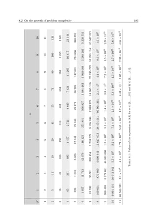
![184 Chapter 8. System Validation
is shown in Figure 8.4. Lastly, the numerical experiments performed later in this chapter reveal
that an MLE response selection feasible search space may actually be chaotic (see §2.2), frag-
mented and possibly disjoint, rather than “smooth” and “predictable.” An artist’s impression
of such a search space is also included in Figure 8.4 [84].
Domain space
Search space
Feasible search space
Figure 8.4: Representations of the domain space, search space and feasible search space of a hypothetical
combinatorial optimisation problem similar to one studied in this dissertation.
8.3 A lower-complexity hypothetical scenario
In order to demonstrate the working of the proposed mathematical modelling subsystem and
optimisation methodology component, described in Chapters 4, 5 and 7, a hypothetical, lower-
complexity deterministic MLE response selection scenario within an intermediate decision mak-
ing paradigm is put forward in this section. The proposed scenario mimics a situation at sea in
which eleven VOIs have been detected and evaluated, after which a decision must be made in
respect of the allocation of MLE resources to these VOIs. Here, the external MLE resource as-
signment infrastructure consists of eight MLE resources, four coastal bases, seven patrol circuits
and three decision making entities. It is assumed that the jurisdiction area is defined analogously
to the EEZ, and that threat detection and threat evaluation input data are available in the MLE
database at the start of the current hypothetical time stage, and that all relevant parameter val-
ues and model management input data have been established. The various parameters relevant
to this scenario together with a formulation of the mathematical model employed are presented
in this section.
8.3.1 Fixed input parameters
In the scenario, eight known threat types are associated with the MLE environment of the
hypothetical coastal nation. In addition, and as mentioned in Chapter 4, the threat evaluation
problem of §8.2.3 into a contingency formulation where each slot may never be assigned more than a certain
number of objects. Although not pursued in this dissertation, it is suggested that this ancillary counting problem
may be solved with the use of generating functions.](https://image.slidesharecdn.com/6cd1ebf5-5cfe-4d40-998c-99cbe17b08f1-170109122537/85/PhD-dissertation-216-320.jpg)
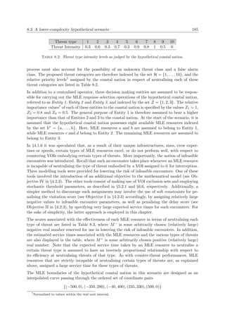
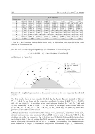
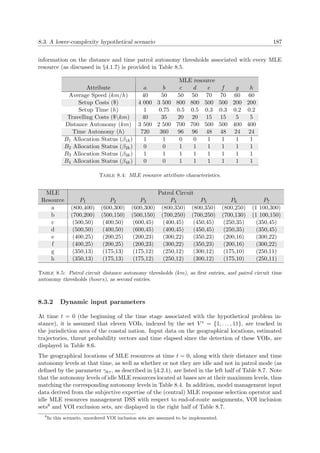
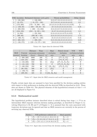
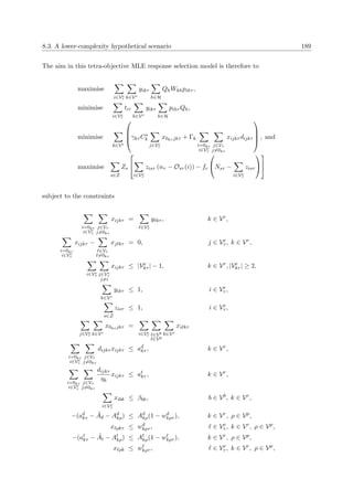
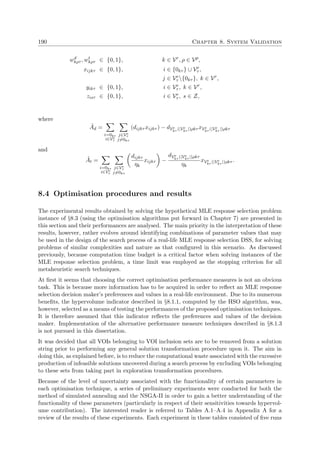
![8.4. Optimisation procedures and results 191
(thus generating five non-dominated fronts in each case) subject to both 1- and 2-minute com-
putational budgets. It should be noted that many more experiments had to be conducted using
the proposed method of simulated annealing (namely 63) due to the relatively large number
of search parameters associated with this method (in contrast to 24 experiments involving the
NSGA-II). Furthermore, for performance assessment purposes, statistics for the average number
of iterations/generations (I and G, respectively), the average size of the non-dominated front
(|A| for the method of simulated annealing and |F1| for the NSGA-II) and the average hypervol-
ume quantity Hvol were recorded for each experiment. In the method of simulated annealing, the
number of iterations refers to the successful number of transformations performed on a solution
throughout the algorithm execution (that is, the total number of feasible neighbour solutions
generated), not to the number of times a solution transformation was applied (irregardless of
the outcome) or to the number of times feasible neighbouring solutions were accepted according
to the Metropolis rule of acceptance.
Based on the output analysis of these preliminary experiments, further robust experiments were
conducted employing well-performing combinations of parametric configurations. These param-
eter value combinations were based on the results in the tables of Appendix A, an understanding
of the nuances associated with the metaheuristics at hand (as discussed in Chapter 2) and sub-
jective choices. Each of these more robust experiments also consisted of five runs each, but
subject to 2- and 5-minute computational budgets instead. The results obtained from any two
experiments within the same termination criterion time frame were compared to one another
by recording their average hypervolume measures (which are to be maximised), as well as their
hypervolume standard deviations, s(Hvol) (which are to be minimised). Here, given a high aver-
age hypervolume associated with any given experiment, a smaller standard deviation around the
expected performance level for the respective search technique and associated parameter value
combination is, of course, more desirable (particularly for risk-averse MLE response selection
decision makers), as it builds up the operator’s confidence in trusting the DSS to produce high-
quality trade-off alternatives to an MLE response selection problem instance every time such a
specifically configured search technique is employed.
The computations required in all experiments were performed on personal computers with 3.0
GHz Intel R CoreTM 2 Duo E8400 processors and 3.25 GB RAM, running in Ubuntu Gnome
3.4.2. The experiments were configured and performed in the software package MATLAB [147].
Due to the nature of the stopping criterion employed in these experiments, care was taken to
ensure that each run was allocated the same processing power for the duration of the search
processes (i.e. the processing power of a computer was not allocated to perform any other
demanding tasks on the same machine).
8.4.1 Objectives normalisation and selection of a reference point
Adopting a reverse engineering approach, numerical bounds associated with each objective func-
tion in this scenario were closely approximated. These bounds are shown in Table 8.9. It is
noted that the lower bounds for Objectives II and III are not zero as the null vector in this
scenario is an infeasible solution.
In order not to favour certain objective functions over others in respect of hypervolume contri-
bution, the points in each non-dominated front were normalised according to the function
f1
norm =
f(x)|1 − f1
min
4.8 − f1
min
along the first objective, where f(x)|1 is the visitation score associated with solution x and f1
min](https://image.slidesharecdn.com/6cd1ebf5-5cfe-4d40-998c-99cbe17b08f1-170109122537/85/PhD-dissertation-223-320.jpg)
![192 Chapter 8. System Validation
Objective Type of bound Numerical bound
Visitation score upper bound 4.8
Total delay lower bound 7.75 (hours)
Operating costs lower bound $5 600
Consensus level upper bound 91
Table 8.9: Approximate evaluation of objective function bounds for the lower-complexity hypothetical
scenario.
is the lowest visitation score recorded in the non-dominated set, the function
f2
norm =
f(x)|2 − 7.75
f2
max − 7.75
along the second objective, where f(x)|2 is the total delay associated with solution x and f2
max
is the highest total delay recorded in the non-dominated set, the function
f3
norm =
f(x)|3 − 5 600
f3
max − 5 600
along the third objective, where f(x)|3 is the operating cost associated with solution x and f3
max
is the highest operating cost recorded in the non-dominated set, and the function
f4
norm =
f(x)|4 − f4
min
91 − f4
min
along the fourth objective, where f(x)|4 is the consensus level associated with solution x and
f4
max is the lowest consensus level recorded in the non-dominated set. The reference point was
chosen as the vector r = (−0.05, 1.05, 1.05, −0.05).
8.4.2 Simulated annealing results
The experiments performed using the multiobjective simulated annealing algorithm proposed
in §7.5 employ four different solution transformation techniques triggered at every iteration
of the algorithm according to a certain probability distribution. These transformations are a
within-route swap transformation with associated probability pwr, a between-route swap transfor-
mation with associated probability pbrs, a between-route delete-and-insert transformation with
associated probability pbrd, and an inter-state transformation with associated probability pis.
Descriptions of the above solution transformations may be found in §7.5.3. In addition, the
exponential growth distribution approach for inter-state transformations was adopted, and so
the parameters (α, β) of §7.5.4 also had to be specified.
The well-known and widely used geometric temperature cooling schedule9 was implemented in
this algorithm due to its simplicity and effectiveness. In this cooling schedule, the temperature
progression is based on the law of geometric decay, described by the function
Tc+1 = πTc,
9
Another successful class of cooling schedules are adaptive schedules, in which regular feedback is received
from the algorithm as a means to evaluate what the next decrement in temperature should be [152]. Such
schedules, however, require a certain parameter determining the change in objective function value at the end of
any given epoch to be defined a priori. Although such a change is easily measurable when solving single-objective
optimisation problems, it is not obvious how this is applicable to multiobjective optimisation problems.](https://image.slidesharecdn.com/6cd1ebf5-5cfe-4d40-998c-99cbe17b08f1-170109122537/85/PhD-dissertation-224-320.jpg)
![8.4. Optimisation procedures and results 193
where Tc is the temperature of the algorithm during search epoch c ∈ {1, . . . , C} and π ∈ (0, 1)
is a constant called the cooling parameter, and where the number of epochs is an indication of
the number of times that the temperature is decreased throughout the algorithm execution (i.e.
the length of each epoch corresponds to the expected number of iterations of the Metropolis
algorithm performed in the inner loop of the method of simulated annealing). This particular
cooling schedule thus provides smaller decrements in temperature as the system approaches a
solidified state. According to Eglese [51], typical values of π employed in practice vary between
0.8 and 0.99.
Given a fixed computation time budget, it is of course noted that thermodynamic equilibrium is
more likely to be reached during any given epoch when C is set lower. Furthermore, because the
stopping criterion employed in these experiments is time elapsed, an interesting property noted
during the implementation of this cooling schedule is that the expected number of iterations
performed during each epoch of the algorithm is determined analogously to the (fixed) fraction
of the total time pre-assigned to each temperature throughout the algorithm. Finally, it must
be pointed out that this cooling schedule is also functional for any computation time budget
budgets, and hence does not necessarily have to be adapted as a function of the allocated
computation time budget.
Because of the large number of parameters that must be defined in this algorithm, the initial
temperature for all experiments was fixed at 30 (this particular initial temperature was found to
work generally well) and the cooling parameter π was selected as either 0.85 or 0.95. The number
of epochs C was assigned the values of 100, 400 and 700, and all four combinations of perturbation
parameters mentioned above were employed, along with three different combination values for
the inter-state parameters (α, β), set at (1.5, 2), (6, 6) and (15, 13). In order to better visualise the
expected proportion of the search spent in each state subspace under these particular numerical
combinations, histograms corresponding to these combinations are provided in Figure 8.6. Note
that, since there are two VOIs belonging to VOI inclusion sets in this scenario, the number of
states in a reduced string will range from 1 to 9.
2 4 6 8
0.0
0.1
0.2
0.3
Steady-stateprobability
State
(a) (α, β) = (1.5, 2)
2 4 6 8
0.00
0.20
0.40
Steady-stateprobability
State
(b) (α, β) = (6, 6)
2 4 6 8
0.00
0.20
0.40
0.60
0.80
Steady-stateprobability
State
(c) (α, β) = (15, 13)
Figure 8.6: Illustrations of steady-state probability distributions for different parametric configurations
of the exponential growth distribution approach for inter-state transformations for the lower-complexity
hypothetical scenario.
Finally, as mentioned previously, each experiment was conducted subject to both 2- and 5-
minute runs. In total, 144 experiments consisting of five runs each were therefore conducted
using the method of simulated annealing. The results of these experiments are tabulated in
Tables 8.10–8.13.
In cases of 2-minute runs, it appears that the majority of the best results (recalling that good
results for a particular experiment are obtained when high hypervolume average with moder-](https://image.slidesharecdn.com/6cd1ebf5-5cfe-4d40-998c-99cbe17b08f1-170109122537/85/PhD-dissertation-225-320.jpg)
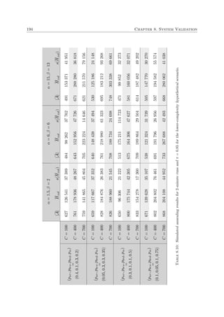
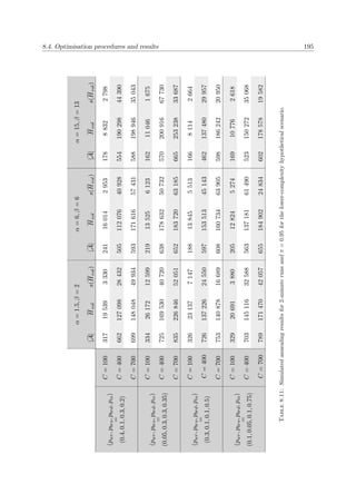
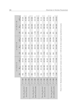
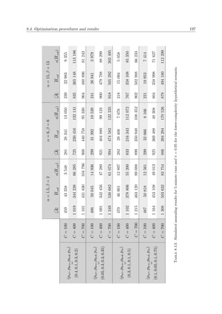
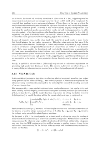
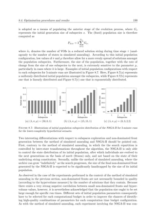
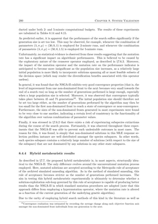
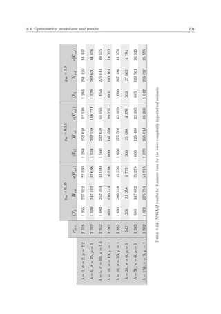
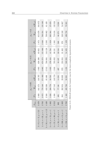
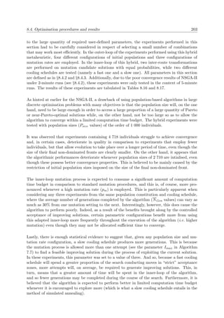
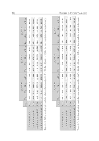
![8.4. Optimisation procedures and results 205
8.4.5 Augmented multistart simulated annealing results
The aim in this section is to investigate whether parallel processing computing attempts are
able to make a significant difference in terms of finding high-quality non-dominated sets of
solutions in comparison to their sequential processing counterparts. To this effect, the augmented
multistart archived simulated annealing algorithm of §7.8 was implemented within a multistart
paradigm, although it is acknowledged that a multistart genetic algorithm may also work very
well. The processors are configured with combinations of the simulated annealing parametric
configurations (deemed to perform relatively well) of §8.4.2.
In addition to the various combinations of archived simulated annealing parameters that may be
used on each processor, a new parameter also has to be considered in these experiments, namely
the number of processors operating in parallel. This is a particularly important decision in the
practical implementation of any real-life DSS, where a trade-off may be pursued between the
expected increased performance linked to the addition of a processor and the additional costs
of setting up, operating and maintaining an additional processor. Aside from the obvious claim
that multistart computing will always perform at least as well as its best-performing processor,
a system engineer will ask himself an important question in this regard, namely what expected
marginal increase in the quantity and quality of non-dominated solutions may be expected
when an additional parallel processor is to be employed in addition to the current ones. This
is, however, not trivial question to answer, as parallel computing involving a fixed number of
processors may perform significantly differently given varying complexity scenarios and varying
algorithm run times.
In order to simulate the parallel computing efficiency in respect of the query above, a basic
multiobjective parallel computing efficiency measure, defined as
ϑ =
Hvol
HP
vol
|A|
N
i=1 |Ai|
= ϑ(Hvol)ϑ(|A|) ∈ (0, 1],
is adopted for the multistart experiments conducted in this chapter. Here, N is the number of
processors employed, HP
vol is an approximation of the hypervolume quantity of the true Pareto
front, while Ai denotes the archive computed by Processor i and A denotes the augmented
archive.
In the above formulation, the metric ϑ(|A|), defined on the interval 1
N , 1 , is a quantification of
the effectiveness of the combined effort of parallel processors to uncover a large number of non-
dominated solutions when pooled together, after duplicate and dominated solutions have been
removed from this pool. In other words, adopting additional processors is more justified if there
are not many solutions in the intersection sets of any two parallel processor archives. Moreover,
the metric ϑ(Hvol), defined on (0, 1], is an approximation of the achievement percentage of
hypervolume of the pooled archive with respect to the estimated maximum hypervolume. As
mentioned before, the true Pareto front is typically not known with certainty, and so neither
is its hypervolume. Noting that underestimating or overestimating its value will not affect the
utility of the metric ϑ significantly in respect of comparing the performance variations when
using different numbers of processors, it is assumed that HP
vol ≈ 2 300 000 (based on the results
obtained earlier in this chapter).
Due to the limitations in computer resources and computer processing power at hand, three
to six runs per experiment were conducted under a computational budget of two minutes only,
the results of which are tabulated in Table 8.18. In this scenario, only two, three and four
processors were tested. Moreover, all processors are assumed to be identical in computing power
and memory capacity and all parameters were defined as in §8.4.2. As expected, this multistart](https://image.slidesharecdn.com/6cd1ebf5-5cfe-4d40-998c-99cbe17b08f1-170109122537/85/PhD-dissertation-237-320.jpg)
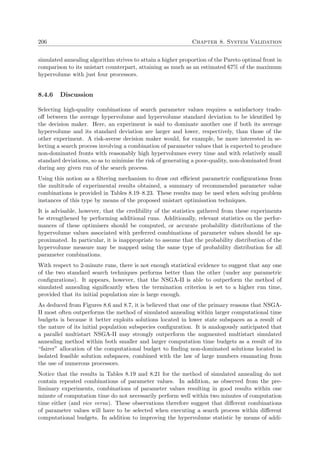
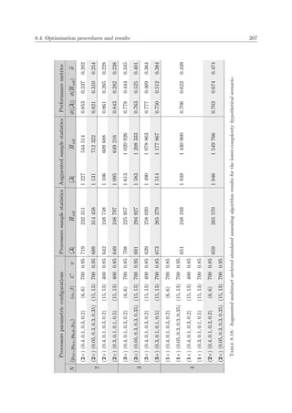
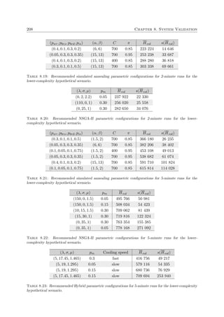
![8.5. A higher-complexity hypothetical scenario 209
tional runs and experimenting with other combinations of parameter values (preferably in the
vicinity of the recommended combinations of parameter values), future work in this area may
focus on analysing the performance of the method of simulated annealing subject to different
computational budgets
Although not pursued in the parallel computing experiments conducted in this chapter, it is
of course perfectly acceptable to strategically combine the results of processors employed to
implement the method of simulated annealing to others employed in implementing the NSGA-
II. This may be achieved similarly to employing the augmented non-dominated front technique
of Algorithm 7.9. A visual test of the merged non-dominated fronts of two processors, each
configured to operate under one of these two algorithms, is portrayed in Figure 8.8. Although
this is just one of countless possible experimental combinations, it is easy to see that both fronts
only rarely intersect, confirming once more that incorporating parallel computing as part of an
MLE response selection DSS may be a good idea.
Finally, due to the type of stopping criterion used in the search processes of these experi-
ments, it is acknowledged that the ability of a search process to perform a certain number of
iterations/generations under a fixed time limit depends on critical factors such as the level of
programming language11 as well as the processing power of the computer(s) employed. Conse-
quently, it is suggested that most of the experiments reported in this chapter ought to perform
significantly better when higher processing power and/or lower complexity languages is imple-
mented.
8.5 A higher-complexity hypothetical scenario
The aim in this section is to assess the performances of some of the proposed search methods
in a more complex environment. More specifically, the hypothetical scenario considered in this
section has been designed to test the ability of selected algorithms to uncover acceptable subsets
of non-dominated solutions from a much larger domain space under a similar computation time
budget.
Threat type MLE resource i
1 (0.5, 0.5)
2 (0.7, 0.3)
3 (0.5, 0.5)
4 (0.2, 0.8)
5 (0.7, 0.3)
6 (0.7, 0.3)
7 (0.8, 0.2)
8 (0.7, 0.3)
9 (0.8, 0.2)
10 (1, 0.1)
Table 8.24: MLE resource i counter-threat ability levels, as first entries, and expected service times
(hours), as second entries.
With only very slight modifications, the hypothetical scenario introduced in this section is
essentially an extension of the lower-complexity scenario of §8.3. This extension consists in
11
It has previously been shown that the time required to perform a fixed series of tasks in a computational
evaluation process may be reduced by more than ten times when a relatively low level of programming language
is employed [16].](https://image.slidesharecdn.com/6cd1ebf5-5cfe-4d40-998c-99cbe17b08f1-170109122537/85/PhD-dissertation-241-320.jpg)
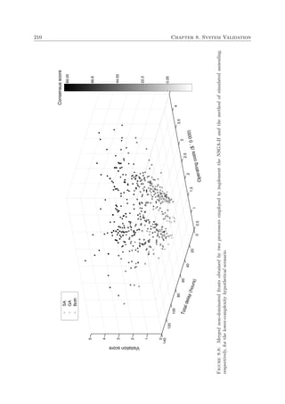
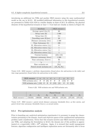
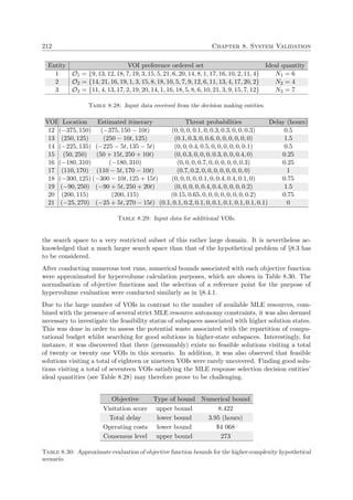
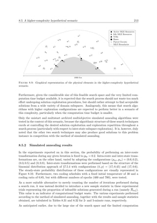
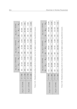
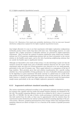
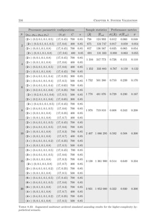
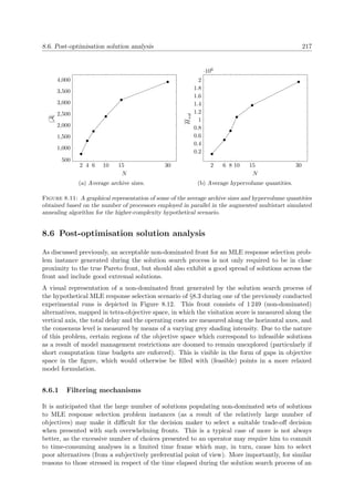
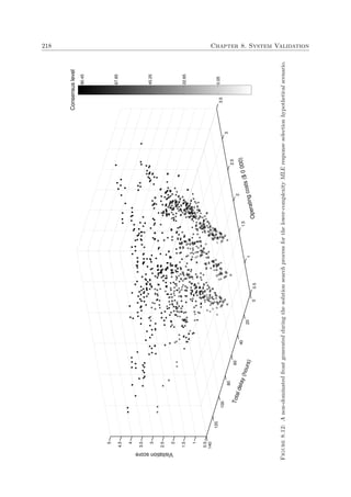
![8.6. Post-optimisation solution analysis 219
MLE response selection problem instance, it is necessary for the decision maker to be able to
select an alternative as rapidly as possible in order to prevent the deterioration of MLE response
selection operations caused by late changes in solution implementation.
It is therefore advocated that one or more filtering mechanisms be employed to reduce the
number of solutions in the non-dominated front a posteriori of the solution search process. An
example of basic filtering techniques may include the use of objective function bounds, where
certain thresholds are specified in order to dismiss certain subsets of points in objective space
(and, of course, the corresponding points in solution space) which violate these thresholds.
To illustrate this filtering technique, consider the following (hypothetical) situation. As a result
of an insufficient budget allocation towards MLE operations, suppose that the operator does
not wish to select alternatives that are expected to cost more than $20 000. Additionally, sup-
pose that the behaviour of more threatening VOIs detected within the jurisdiction area of the
hypothetical coastal nation is often unpredictable and intelligent, to the extent that they have
in the past often managed to escape from the tracking of threat detection systems as a result
of late servicing. The operator may wish to remedy to this problem by ignoring solutions that
generate excessively large delay scores, and decide to impose a total delay upper bound score of
100 hours. Lastly, in order to remain on good terms with the decentralised MLE response se-
lection decision making entities with whom he collaborates, as well as to take into account their
expert advice in respect of which detected VOIs they reckon they are competent to investigate,
the (central) operator may decide only to consider solutions associated with a consensus level of
at least 40 points. The result of the above-mentioned impositions placed on the non-dominated
front of Figure 8.12 is portrayed in Figure 8.13. For visual purposes, note that the spectrum of
grey intensities quantifying the fourth objective has been rescaled.
Here, it is interesting to point out that there exists a strong correlation between the visitation
score and the consensus level (i.e. the higher the solutions are mapped on the visitation score
axis, the darker they seem to be). This is because the cumulated ideal quantity of VOIs of the
hypothetical MLE response selection scenario of §8.3 amounts to 10, and so solutions residing in
higher state subspaces are generally preferred by the decision making entities (that is, provided
that the correct assignment of VOIs to entities is performed).
The implementation of these objective bounds allowed for the original non-dominated set to be
reduced by over 50%, rendering the subsequent selection process easier. Of course, the stricter
these objective bounds are, the more reduced the non-dominated set will be. However, even after
the use of this kind of filter, there may still be too many alternatives. A more sophisticated
procedure is the -filter technique [167], which aims to partition areas of high solution density
by slicing objective function ranges of values at regular intervals in order to form M-orthotopes
in the M-dimensional objective space. A single non-dominated point, located in each orthotope,
is then retained, provided that there is at least one point in the orthotope, while the remaining
points are removed from the front and solution space.
To better describe this filtering process, consider Figure 8.14 in which a non-dominated front has
been generated for solving a bi-objective minimisation problem with objective functions f1 and
f2. Here, the parameters 1 and 2 are used to partition the objective function ranges at regular
intervals into regular intervals of lengths 1 and 2, respectively, and discarding solutions so that
only one point in each of the resulting cross-sectional rectangles remains. Of course, the larger
the parameter values 1 and 2 are, the smaller the remaining number of non-dominated solutions
will be. In particular, it is noted that | ˜F | → | ˜F| as 1, . . . , M → 0 (where ˜F represents the
resulting -filtered non-dominated front).
To illustrate the functionality of the above-mentioned filtering mechanism in a more complex](https://image.slidesharecdn.com/6cd1ebf5-5cfe-4d40-998c-99cbe17b08f1-170109122537/85/PhD-dissertation-251-320.jpg)
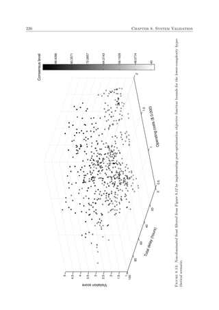
![8.6. Post-optimisation solution analysis 221
f1
f2
2
1
(a) Non-dominated front before implementing
the -filter technique.
f1
f2
2
1
(b) Non-dominated front after implementing the
-filter technique.
Figure 8.14: Application of the -filter technique to the non-dominated front of a bi-objective minimi-
sation problem with objective functions f1 and f2.
objective space environment, reconsider the (reduced) non-dominated front of Figure 8.13, and
suppose that the -filter technique is applied with -values ( 1, 2, 3, 4) ≈ (1, 25, 500, 12.5).
The resulting (reduced) non-dominated front generated as a result of this process is shown
in Figure 8.15. Here, each objective function range was sliced exactly three times, creating
44 = 256 4-orthotopes across the objective space. Although certain clusters of points may seem
too “close” to one another in respect of the three-dimensional Euclidean objective space, the
reader is reminded that, in such cases, the closeness of these points differ largely in their values
of the fourth objective function (i.e. significantly different shades of grey are observed amongst
these points).
The filtered non-dominated front obtained by applying these two filtering techniques in com-
bination produces a total of fifty one non-dominated solutions, which clearly is a significant
improvement over the initial non-dominated front (over twenty four times smaller than the
initial number of non-dominated solutions). For the sake of clarity, these points may also be
projected orthogonally from three-dimensional Euclidean objective space (i.e. considering the
first three objectives only) onto the three two-dimensional planes, as shown in Figure 8.16.
Although not portrayed here, the more advanced cluster filtering techniques may also be em-
ployed by grouping non-dominated points into clusters in such a way that any two alternatives
in a specific cluster are sufficiently “similar” to one another while being sufficiently “different”
to the alternatives included in other clusters [73, 110]. One representative in each cluster (e.g.
its centroid) may then be retained, representing the characteristics of the cluster as a whole,
while the other points in that cluster are discarded. In [110], for instance, a filtering technique
referred to as subspace clustering is employed, which is an extension of traditional clustering
that seeks to find clusters in different subspaces within a data set made up of highly-dimensional
observations (such as the set of non-dominated solutions mapped in objective space in an MLE
response selection problem).](https://image.slidesharecdn.com/6cd1ebf5-5cfe-4d40-998c-99cbe17b08f1-170109122537/85/PhD-dissertation-253-320.jpg)
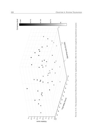
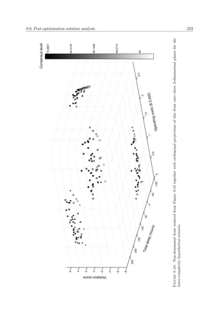
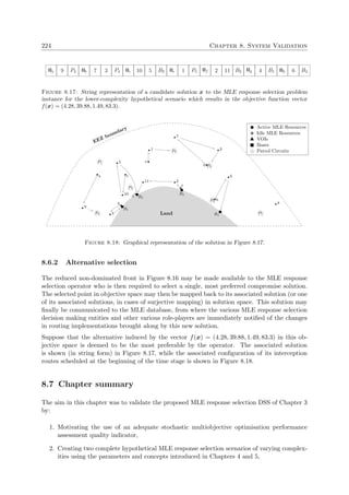

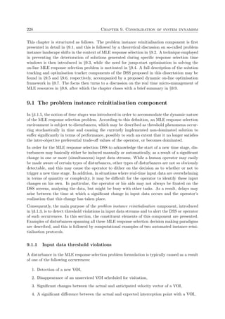
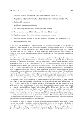
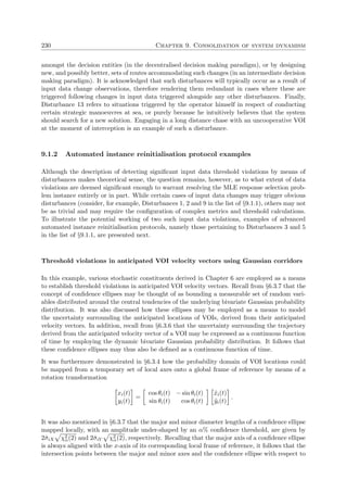
![9.1. The problem instance reinitialisation component 231
the global frame of reference are given by the two-dimensional coordinates
P −
maj(xi), P −
maj(yi) (t) =
µiX(t)
µiY (t)
−
cos θi(t) − sin θi(t)
sin θi(t) cos θi(t)
˘σiX(t) χ2
α(2)
0
=
µiX(t) − ˘σiX(t) χ2
α(2) cos θi(t)
µiY (t) − ˘σiX(t) χ2
α(2) sin θi(t)
and
P +
maj(xi), P +
maj(yi) (t) =
µiX(t) + ˘σiX(t) χ2
α(2) cos θi(t)
µiY (t) + ˘σiX(t) χ2
α(2) sin θi(t)
along the major axis of the confidence ellipse, and (similarly)
P −
min(xi), P −
min(yi) (t) =
µiX(t)
µiY (t)
−
cos θi(t) − sin θi(t)
sin θi(t) cos θi(t)
0
˘σiY (t) χ2
α(2)
=
µiX(t) + ˘σiY (t) χ2
α(2) sin θi(t)
µiY (t) − ˘σiY (t) χ2
α(2) cos θi(t)
.
and
P +
min(xi), P +
min(yi) (t) =
µiX(t) − ˘σiY (t) χ2
α(2) sin θi(t)
µiY (t) + ˘σiY (t) χ2
α(2) cos θi(t)
.
along the minor axis of the confidence ellipse. A subset of these coordinates are shown in
Figure 9.1.
E[(Xi, Yi)t]
fN(xi,yi)t
P −
min(xi)
P +
min(xi)
P −
maj(yi)
P +
maj(yi)
yi
xi
Figure 9.1: Intersection coordinates between the diameters and contour of a confidence ellipse.
The dynamic bivariate Gaussian probability distribution modelling the anticipated trajectory of
a VOI may be represented visually by super-positioning an infinite number of consecutive bivari-
ate Gaussian distributions over a vector trajectory consisting of anticipated central tendencies
mapped in a bounded space-time continuum. To this effect, define the Gaussian corridor G of a
VOI as the space-time mapping of the dynamic bivariate Gaussian distribution of its anticipated
locations over a specific time interval. This corridor may be employed to model the displace-
ment of a Gaussian random variable governed by a dynamic bivariate Gaussian distribution as
a function of time. Moreover, define the α-bounded Gaussian corridor G(α, i) of VOI i as the](https://image.slidesharecdn.com/6cd1ebf5-5cfe-4d40-998c-99cbe17b08f1-170109122537/85/PhD-dissertation-263-320.jpg)
![232 Chapter 9. Consolidation of system dynamism
space-time mapping of the confidence ellipses derived from the underlying distribution over a
specific time interval. The space enclosed by these boundaries is then defined by the confidence
ellipse contour coordinates (derived above) over that time interval.
This notion is best demonstrated by means of a simple example. Consider some VOI i at the
beginning of a time stage with estimated initial position (Xi, Yi)0 = (50, 60), static anticipated
velocity vector (see §6.3.2) ˜vi = [θi si] = [ π
12 10], and corresponding anticipated location vector
˜i(t) = 50 + 10t cos
π
12
, 60 + 10t sin
π
12
≈ (50 + 9.7t, 60 + 2.6t).
Moreover, suppose that the error associated with the anticipated location of this VOI as a
function of time is estimated by means of the variance functions ˘σ2
iX(t) = 0.2+1.5t and ˘σ2
iY (t) =
0.15 + 0.8t (see §6.3.4), and assume that temporal projections on the anticipated locations of
this VOI are only required up to three hours from time t = 0. Suppose further that the operator
wishes to configure the Gaussian corridor of this VOI in such a way that there is no more than an
estimated 10% chance that the actual trajectory of this VOI will exit this corridor at any point
during the course of the following three hours. Noting that χ2
90(2) ≈ 4.61 and recalling that the
vector of central tendencies µi(t) is presumably given by ˜i(t), the boundaries of this Gaussian
corridor along the minor diameters of the confidence ellipses are therefore approximated by the
set of parametric equations
G(α, i)−
min = P −
min(xi), P −
min(yi) (t)
=
50 + 9.7t + (0.15 + 0.8t)
√
4.61 sin π
12
60 + 2.6t − (0.15 + 0.8t)
√
4.61 cos π
12
≈
50.16 + 10.56t
59.72 + 1.11t
and
G(α, i)+
min = P +
min(xi), P +
min(yi) (t)
=
50 + 9.7t − (0.15 + 0.8t)
√
4.61 sin π
12
60 + 2.6t + (0.15 + 0.8t)
√
4.61 cos π
12
≈
49.84 + 8.84t
60.16 + 3.46t
for all t ∈ [0, 3]. These equations may alternatively be expressed in terms of the global frame
of reference as G(α, i)−
min : yi ≈ 0.11xi + 54.42 and G(α, i)+
min : yi ≈ 0.39xi + 40.65 for all
xi ∈ [50, 70.1]. The set of parametric equations G(α, i)−
maj and G(α, i)+
maj may be derived
similarly.
An approximate graphical depiction of this Gaussian corridor is shown in Figure 9.2 and its spa-
tial projection is elucidated in Figure 9.3. A case of disturbance is also illustrated in Figure 9.2,
where the actual trajectory of VOI i, i(t), exits the Gaussian corridor at time t = 2.4 hours
approximately.
Although this example represents a simple case of an anticipated VOI trajectory, which allows
for an easy visual representation of its corresponding Gaussian corridor, it is noted that the
underlying geometrical shape of hyper-dimensional Gaussian corridors becomes rather tedious
when dealing with non-linear velocity vector parametric equations. Finally, it is noted that
α-bounded Gaussian corridors need not only be derived from a continuous bivariate Gaussian
distribution. If only a time series of discrete Gaussian distributions is employed instead (see
§6.3.4), then the corresponding Gaussian corridor may simply be extrapolated approximately
from the edges of the underlying (discrete) confidence ellipses.](https://image.slidesharecdn.com/6cd1ebf5-5cfe-4d40-998c-99cbe17b08f1-170109122537/85/PhD-dissertation-264-320.jpg)
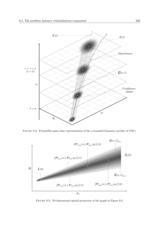
![234 Chapter 9. Consolidation of system dynamism
Threshold violations in VOI threat probabilities using the weighted p-norm
Disturbances caused by significant updates of the threat probability vector of a VOI may cause
a scheduling problem for the MLE resource assigned to intercept it. If H is the set of indices
representing each type of threat faced by the coastal nation (as defined in Chapter 4), then let
pt
i = [pt
i1, . . . , pt
i|H|] be the threat probability vector of VOI i ∈ Ve
τ at time t ∈ , and define
the weighted p-norm of the difference between the threat probability vector of VOI i at the
beginning of the current time stage and at present time as
p0
i − pt∗
i
p
=
h∈H
Qh p0
ih − pt∗
ih
p
1
p
,
where p ≥ 1 (by definition of the standard p-norm), t∗ > 0 and Qh represents the priority level
assigned by the coastal nation to neutralise class h threats (as described in §4.2.1). The output
given by the proposed weighted p-norm is therefore more sensitive to changes in probabilities
associated with threats subject to higher priority levels. Henceforth, define ∆p ∈ (0, 1) as a
pre-determined threshold set by the operator in the sense that the subsystem is configured to
trigger a disturbance (and immediately inform the operator in real time) if there exists a VOI
i ∈ Ve
τ for which p0
i − pt∗
i p
> ∆p at any time t∗.
9.2 Problem instance landscape shifts
In dynamic on-line optimisation problems, specific deviations in input data ought to affect the
geometry of the decision and objective spaces in certain ways. It may thus be beneficial to
understand how these spaces tend to transition as a result of these changes for the purpose
of, for example, selecting adequate problem instance reinitialisation optimisation methods best
able to re-track a shifted Pareto front. This metamorphosis of the problem instance nature is
referred to here as landscape shifts.
Because every problem instance is different and every change in input data is unique, however,
it may not be practical to analyse specific problem instance landscape shifts every time these
manifest themselves. Instead, the aim in this section is to put forward a generic classification
of problem instance landscape shifts that may be employed in multiobjective dynamic on-line
optimisation problems, and to elucidate these categories with examples of input data variations
that may occur within the MLE response selection DSS proposed in this dissertation.
Problem landscape shift category 1 2 3 4 5 6
The previous feasible decision space remains entirely feasible and valid? × × ×
None of the previous solutions are affected in objective space? × × × ×
Some of the previous solutions are affected across all objectives at once? × × × ×
Table 9.1: General categories of multiobjective optimisation landscape shifts (× = no; = yes).
Six categories of MLE response selection landscape shifts are considered in this section; these
are summarised in Table 9.1. Here, a solution to an MLE response selection problem instance is
defined to be invalid if it no longer forms part of the domain space (S) of the instance; that is, if
it is no longer applicable to the current situation. For the sake of illustration, a centralised MLE
response selection decision making paradigm involving Objectives I (visitation score), II (total](https://image.slidesharecdn.com/6cd1ebf5-5cfe-4d40-998c-99cbe17b08f1-170109122537/85/PhD-dissertation-266-320.jpg)
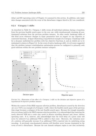
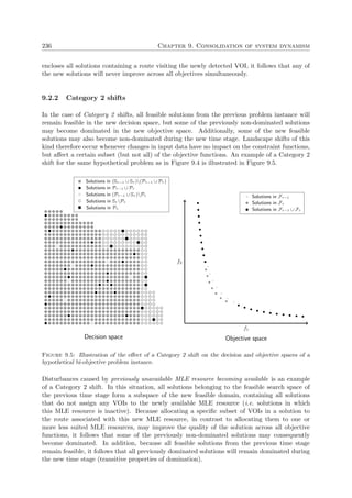
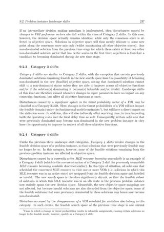
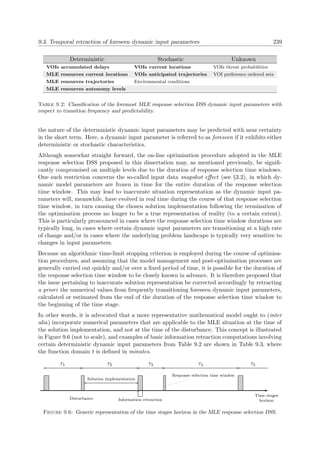
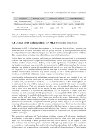
![9.5. The solution tracking component 241
In other words, numerous consecutive “small” but accumulating landscape shifts are actually
bound to occur between any two problem instance reinitialisations, and so tracking the shift in
Pareto-optimal solutions may not be as simple as suggested in §9.2, but may rather be a com-
pounded accumulation of many landscape shifts of different categories and different intensities.
An approximated Pareto optimal set may consequently not be useful in jump-start optimisa-
tion procedures if it is not tracked efficiently, particularly if input data variations are generally
frequent and disturbances are far apart.
Generic jump-starting techniques for dynamic multiobjective VRPs are, however, very scarce
in the literature, and most related studies only tend to give examples for simplified, generic
mathematical models. In agreement with C´amara et al. [20], the author consequently specu-
lates that there exists no common, unified structure for solving the like of the MLE response
selection problem in a dynamic fashion. In the following three sections, the solution tracking
and optimisation tracker components are therefore presented in some detail with the aim of
associatively structuring a functional jump-starting optimisation framework for use in problem
instance reinitialisation procedures.
9.5 The solution tracking component
In order to carry over a chosen set of solutions from one time stage to the next, it is necessary to
continually evolve these solutions in both decision and objective space. This process is referred to
here as solution tracking, which takes place in the solution tracking component of the information
management subsystem introduced in §3.1.3.
The solutions to be tracked need not only consist of a current estimate of the Pareto-optimal set
˜Pτ (which, of course, also contains the currently chosen solution for implementation), but may
also consist of a mutually exclusive set of strategically (or randomly) retained dominated and
infeasible solutions, defined here as Dτ . Examples of elements that may be appended to this set
include extreme solutions, solutions promoting diversity, isolated solutions in objective space,
solutions belonging to second or third non-dominated fronts, and infeasible solutions closely
located to feasible domain subspaces of interest in decision space.
9.5.1 The solution tracking algorithm
Solution tracking is a simple, low complexity process, which works as follows. Updates in input
data variations that have ensued since the start of the previous solution tracking time interval,
referred to here as a time split, are first received from external data sources at the start of the
current time split (if any3). Unlike the conditions necessary to trigger disturbances (as discussed
in §9.1), however, these input data updates account for any changes in problem formulation,
no matter how small (such as the accurate monitoring of the updated geographical positions of
VOIs and MLE resources). Solutions that are both in ˜Pτ and Dτ are first assessed for invalidity
(recalling that a solution is classified as invalid if it does not form part of the current problem
domain). Consider, for example, solutions scheduled to visit a VOI which no longer belongs to
the set Ve
τ after it was serviced during the course of the current time stage.
Next, solutions in ˜Pτ are reassessed for feasibility in decision space, taking into consideration
the possible domain landscape shifts that have transpired since the start of the previous time
split. Based on the chosen configuration, infeasible solutions in ˜Pτ are then either transferred to
3
In cases where the duration of a time split is quicker than the rate of input data updates, for example.](https://image.slidesharecdn.com/6cd1ebf5-5cfe-4d40-998c-99cbe17b08f1-170109122537/85/PhD-dissertation-273-320.jpg)
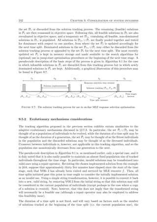

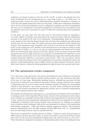
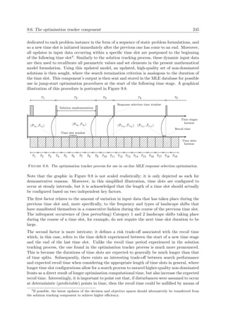
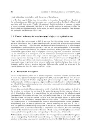
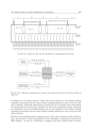
![250 Chapter 9. Consolidation of system dynamism
(a) Technical information pertaining to an MLE
resource.
(b) Radar information for detecting and tracking
objects at sea.
Figure 9.11: Examples of HMI displays that may be found on board MLE resources.
resource course and speed adjustments are bound to be made throughout solution implementa-
tion operations. In addition, and as discussed in §6.5, not only should the servicing of VOIs be
conducted effectively, but also as quickly as possible. These operational manoeuvres ultimately
ought to be conducted in a way that agrees with the MLE response selection goals pursued by
the coastal nation. In particular, although efficient microscopic decision making6 of this kind
will not affect the visitation score or consensus level, it may very well reduce operating costs
and total delay time, thus pursuing Objectives II and III of Chapter 4.
9.9 Chapter summary
In the first section of this chapter, the problem instance reinitialisation component of the MLE
response selection DSS put forward in this dissertation was described in detail using various
examples of disturbances and reinitialisation protocols. A theoretical discussion pertaining to
the shift in decision and objective space of a problem instance as a result of input data variations
was then conducted in §9.2, and this was followed in §9.3 by a description of the technique of
temporal retraction of foreseen dynamic input parameters, and an analysis of the jump-start
optimisation prerequisites required for solving the MLE response selection problem in an on-line
fashion in §9.4. Full descriptions of the solution tracking and optimisation tracker components of
the proposed DSS were provided in §9.5 and §9.6, respectively, after which an on-line, dynamic
optimisation framework for fusing the results of these two components together was proposed in
§9.7. Finally, the role of MLE resources in making effective micro-decisions in agreement with
the goals of the coastal nation was explained in §9.8.
6
Auxiliary objectives of this kind are often referred to as mean objectives in the literature [27].](https://image.slidesharecdn.com/6cd1ebf5-5cfe-4d40-998c-99cbe17b08f1-170109122537/85/PhD-dissertation-282-320.jpg)
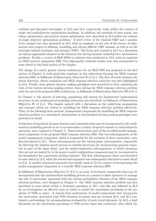
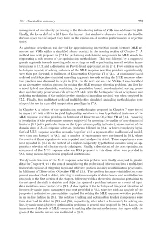

![10.3. Dissertation contributions 255
10.3 Dissertation contributions
The main contributions of this dissertation are fivefold, as outlined in this section.
Following the review in Chapter 2 of MLE DSSs in existence, it was acknowledged that very few
studies tend to focus on the MLE response selection process for active MLE resources in real
time, and no previous studies were found in the literature for solving the MLE response selection
problem as a combinatorial optimisation problem using the analogy of the dynamic VRP as a
means to model the problem. In addition, most of the existing studies were conducted within
the context of the environment of a specific coastal nation and thus tend to not be formulated
in a generic manner. The first contribution of this dissertation therefore centres around the
design of a novel, generic MLE response selection DSS and overall MLE system architecture, as
proposed in Chapter 3. In this design, it was acknowledged that the MLE response selection
operations of a coastal nation are typically not conducted via a single central operator (or group
of central operators) assisted by a single DSS, but are rather orchestrated by multiple, and often
to some degree independent, role players. Consequently, three suitable paradigms of decision
entity autonomy, inspired by the notion of the processing of information in VRPs (as described in
§2.6) were proposed in which the MLE response selection framework may function in a practical
manner.
The second contribution was the combinatorial optimisation model formulation of a new kind of
dynamic multiobjective VRP (defined in the dissertation as the MLE response selection routing
problem) in Chapter 4, in which the depots represent the bases from whence MLE resources are
dispatched, the fleet of vehicles represents the fleet of MLE resources at the collective disposal of
the decision entities and the customers represent the VOIs tracked at sea within the territorial
waters of the coastal nation. The formulation of the MLE response selection problem therefore
incorporates a unique feature combination of a heterogeneous fleet of vehicles, multiple depots,
customer profits, asymmetric travel arc lengths and dynamic customer locations. In addition,
the nature of information specification in this problem is classified as both dynamic (i.e. certain
input data are made known to the operator/decision maker in a continual fashion) and stochastic
(i.e. certain input data are estimated or prescribed as probability distributions). Various deter-
ministic fixed and dynamic features of the MLE response selection problem were identified in
Chapters 4 and 5, and incorporated into the mathematical modelling subsystem of the DSS. A
selection of the fundamental modelling features have been published in [32], while a selection of
the dynamic modelling features were published in [33]. Additionally, various stochastic features
of the MLE response selection problem were derived in Chapter 6, and also incorporated into
the mathematical modelling subsystem of the DSS.
The third contribution of this dissertation involves the incorporation of an array of various
intricate features associated with the nature of the MLE response selection problem into the
optimisation methodology component, as described in Chapter 7. In particular, the following
solution search aspects had to be designed by hand:
1. An algebraic description of a methodology for approximating interception points between
MLE resources and VOIs when subject to trajectory deviations caused by environmental
vectors.
2. A generic, practical representation of solutions to MLE response selection problem in-
stances, as well as a general process for transforming solutions during a search process
which accommodates both fixed and dynamic modelling features (this work has also been
published in [33]).](https://image.slidesharecdn.com/6cd1ebf5-5cfe-4d40-998c-99cbe17b08f1-170109122537/85/PhD-dissertation-287-320.jpg)

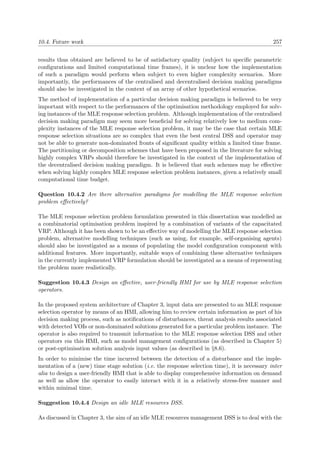
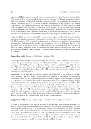
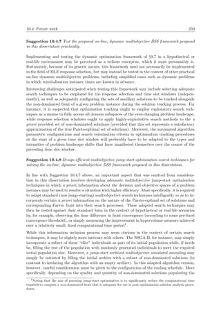

![References
[1] Archetti C, Speranza M & Vigo D, 2012, Vehicle routing problems with profits,
(Unpublished) Technical Report, Department of Economics and Management, University
of Brescia, Brescia.
[2] ASTUTE, 2014, United Nations Convention on the Law of the Sea, [Online], [Cited
December 19th, 2014], Available from http://www- dsp.elet.polimi.it/ispg
/ASTUTE/wiki/doku.php?id=d22:information retrieval and fusion:
multimodal information fusion.
[3] B¨ack T, 1994, Selective pressure in evolutionary algorithms: A characterization of se-
lection mechanisms, Proceedings of the First IEEE Conference on Computational Intel-
ligence, pp. 57–62.
[4] Banos R, Ortega J, Gil C, Fernandez A & De Toro F, 2013, A simulated
annealing-based parallel multi-objective approach to vehicle routing problems with time
windows, Expert Systems with Applications, 40(5), pp. 1696–1707.
[5] Bar´an B & Schaerer M, 2003, A multiobjective ant colony system for vehicle routing
problem with time windows, Proceedings of the 2003 International Conference on Applied
Informatics, pp. 97–102.
[6] Bashir F, Khokhar A & Schonfeld D, 2007, Object trajectory-based activity clas-
sification and recognition using hidden Markov models, IEEE Transactions on Image
Processing, 16(7), pp. 1912–1919.
[7] Blum C & Roli A, 2003, Metaheuristics in combinatorial optimization: Overview and
conceptual comparison, Journal of ACM Computing Surveys, 35(3), pp. 268–308.
[8] Borgerson SG, 2009, The national interest and the Law of the Sea, Council on Foreign
Relations Press No. 46, Washington (DC).
[9] Bouejla A, Chaze X, Guarnieri F & Napoli A, 2014, A Bayesian network to
manage risks of maritime piracy against offshore oil fields, Journal of Safety Science, 68,
pp. 222–230.
[10] Bowden A, 2010, The economic costs of maritime piracy, (Unpublished) Technical Re-
port, One Earth Future Foundation, Louisville (CO).
[11] Box GE, 1979, Robustness in the strategy of scientific model building, Journal of Ro-
bustness in Statistics, 1, pp. 201–236.
[12] Branke J, 1999, Memory enhanced evolutionary algorithms for changing optimization
problems, Congress on Evolutionary Computation, 3, pp. 1875–1882.
[13] Branke J, Kaußler T, Smidt C & Schmeck H, 2000, A multi-population approach
to dynamic optimization problems, Springer, London.
261](https://image.slidesharecdn.com/6cd1ebf5-5cfe-4d40-998c-99cbe17b08f1-170109122537/85/PhD-dissertation-293-320.jpg)
![262 REFERENCES
[14] Bressen T, 2007, Consensus decision making: What, why, how, Berrett-Koehler Pub-
lishers, San Francisco (CA).
[15] Bromiley P, 2003, Products and convolutions of gaussian probability density functions,
Tina-Vision Memo, 3, pp. 2–7.
[16] Burger AP, 2014, University of Stellenbosch, [Personal Communication], Contactable
at apburger@sun.ac.za.
[17] Burke EK & Kendall G, 2005, Search methodologies, Springer Science & Business
Media Incorporated, New York (NY).
[18] Busetti F, 2003, Simulated annealing overview, [Online], [Cited June 2nd, 2013], Avail-
able from http://www.geocities.%20com/francorbusetti/saweb.
[19] Bynum WF, 2009, The origin of species by means of natural selection: Or, the preser-
vation of favored races in the struggle for life, AL Burt, New York (NY).
[20] C´amara M, Ortega J & De Toro F, 2010, Approaching dynamic multi-objective
optimization problems by using parallel evolutionary algorithms, Springer, Berlin.
[21] C´amara M, Ortega J & De Toro F, 2007, Parallel processing for multi-objective op-
timization in dynamic environments, Proceedings of the IEEE International Symposium
on Parallel and Distributed Processing, pp. 1–8.
[22] Cape Town Green Map, 2013, City takes its marine and environmental law enforce-
ment unit to the next level, [Online], [Cited January 26th, 2013], Available from http:
//www.capetowngreenmap.co.za/blog/city-takes-its-marine-and-environmental-
law-enforcement-unit-next-level.
[23] Castro JP, Landa-Silva D & P´erez JAM, 2009, Exploring feasible and infeasible
regions in the vehicle routing problem with time windows using a multi-objective particle
swarm optimization approach, Springer, Berlin.
[24] Chakraborty N, 2004, Genetic algorithms in materials design and processing, Inter-
national Materials Reviews, 3, pp. 246–260.
[25] Chen P & Xu X, 2008, A hybrid algorithm for multi-depot vehicle routing problem, Pro-
ceedings of the 2008 IEEE International Conference on Service Operations and Logistics,
and Informatics, pp. 2031–2034.
[26] Clarke G & Wright JW, 1964, Scheduling of vehicles from a central depot to a number
of delivery points, Operations Research, 12(4), pp. 568–581.
[27] Clemen R & Reilly T, 2001, Making hard decisions with decision tools, Duxbury,
Belmont (CA).
[28] Cobb HG & Grefenstette JJ, 1993, Genetic algorithms for tracking changing envi-
ronments, (Unpublished) Technical Report, Naval Research Lab, Washington (DC).
[29] Coello CA, Lamont GB & van Veldhuizen DA, 2007, Evolutionary algorithms for
solving multi-objective problems, 2nd Edition, Springer Science & Business Media, New
York (NY).
[30] Collins English Dictionary, 2013, Decide, [Online], [Cited September 4th, 2013],
Available from http://dictionary.reference.com/browse/decide.
[31] Collins english dictionary, 2014, Metaheuristic, [Online], [Cited September 23rd,
2014], Available from http://dictionary.reference.com/browse/metaheuristic.
[32] Colmant A and van Vuuren JH, 2013, Prerequisites for the design of a maritime
law enforcement resource assignment decision support system, Proceedings of the 42nd
Annual Conference of the Operations Research Society of South Africa, pp. 90–101.](https://image.slidesharecdn.com/6cd1ebf5-5cfe-4d40-998c-99cbe17b08f1-170109122537/85/PhD-dissertation-294-320.jpg)
![REFERENCES 263
[33] Colmant A and van Vuuren JH, 2014, Solution representation for a maritime law
enforcement response selection problem, Proceedings of the 43rd Annual Conference of
the Operations Research Society of South Africa, pp. 79–87.
[34] Colmant A, 2012, A simulation study of the impact of lead time on the costs of deliv-
eries, BComm Honnours Project, University of Stellenbosch, Stellenbosch.
[35] Czyz˙zak P & Jaszkiewicz A, 1998, Pareto simulated annealing: A metaheuristic tech-
nique for multiple-objective combinatorial optimization, Journal of Multi-Criteria Deci-
sion Analysis, 7(1), pp. 34–47.
[36] Dabrowski JJ & De Villiers JP, 2014, Maritime piracy situation modelling with
dynamic Bayesian networks, Journal of Information Fusion, 23, pp. 116–130.
[37] Dantzig GB & Ramser JH, 1959, The truck dispatching problem, Management Science,
6(1), pp. 80–91.
[38] Darby-Dowman K, Fink RK, Mitra G & Smith JW, 1995, An intelligent system
for US Coast Guard cutter scheduling, European Journal of Operational Research, 87,
pp. 574–585.
[39] De Seligny J & Grainger R, 2010, The state of world fisheries and aquaculture, Food
and Agriculture Organization of the United Nations, Rome.
[40] Deb K & Goel T, 1999, Evolutionary multi-criterion optimization, Evolutionary Algo-
rithms in Engineering and Computer Science, 1, pp. 135–162.
[41] Deb K, Pratap A, Agarwal S & Meyarivan T, 2002, A fast and elitist multiobjective
genetic algorithm: NSGA II , Evolutionary Computation on IEEE Transactions, 6(2),
pp. 182–197.
[42] Deb K, 2001, Multi-objective optimization using evolutionary algorithms, John Wiley &
Sons, Beijing.
[43] Dembczy´nski K, Kotlowski W & Slowi´nski R, 2006, Additive preference model with
piecewise linear components resulting from dominance-based rough set approximations,
Springer, Berlin.
[44] Deshpande S, Watson L & Canfield R, 2013, Pareto front approximation using a
hybrid approach, Procedia Computer Science, 18, pp. 521–530.
[45] Diaz-Gomez PA & Hougen DF, 2007, Initial population for genetic algorithms: A
metric approach, Proceedings of the 2007 International Conference on Genetic and Evo-
lutionary Methods, pp. 43–49.
[46] Diffen, 2016, Goal vs. Objective, [Online], [Cited February 15th, 2015], Available from
http://www.diffen.com/difference/Goal vs Objective.
[47] Dorigo M & Gambardella LM, 1997, Ant colony system: A cooperative learning
approach to the traveling salesman problem, IEEE Transactions on Evolutionary Com-
putation, 1(1), pp. 53–66.
[48] Dr´eo J, 2006, Metaheuristics for hard optimization: Methods and case studies, Springer,
Paris.
[49] Du Toit J, 2014, Decision support for threat detection in maritime surveillance, PhD
Dissertation, University of Stellenbosch, Stellenbosch.
[50] Eberhart RC & Kennedy J, 1995, A new optimizer using particle swarm theory,
Proceedings of the 6th International Symposium on Micro Machine and Human Science,
1, pp. 39–43.](https://image.slidesharecdn.com/6cd1ebf5-5cfe-4d40-998c-99cbe17b08f1-170109122537/85/PhD-dissertation-295-320.jpg)
![264 REFERENCES
[51] Eglese R, 1990, Simulated annealing: A tool for operational research, European Journal
of Operational Research, 46(3), pp. 271–281.
[52] Encyclopaedia Britannica, 2015, Law of large numbers, [Online], [Cited March 22nd,
2016], Available from http://global.britannica.com/science/law-of-large-
numbers.
[53] EPFL, 2015, Conditional Probability, [Online], [Cited March 14th, 2016], Available from
http://statwww.epfl.ch/davison/teaching/ProbStatSC/20032004/week4and5.pdf.
[54] Farahbod R, Glasser U & Khalili A, 2009, A multi-layer network architecture for
dynamic resource configuration and management of multiple mobile resources in maritime
surveillance, International Society for Optics and Photonics, 7345, pp. 734508–734508.
[55] Farina A, Giompapa S, Gini F, Graziano A & Stefano RD, 2007, Computer
simulation of an integrated multi-sensor system for maritime border control, Proceedings
of the 2007 IEEE Radar Conference, pp. 308–313.
[56] Farina M, Deb K & Amato P, 2004, Dynamic multiobjective optimization problems:
Test cases, approximations, and applications, IEEE Transactions on Evolutionary Com-
putation, 8(5), pp. 425–442.
[57] Fisheries and Oceans Canada, 2013, Canada to extend life of coast guard fleet, [On-
line], [Cited February 22nd, 2013], Available from http://www.worldmaritimenews.com
/archives/77223/canada-to-extend-life-of-coast-guard-fleet/.
[58] Fonseca CM, Knowles JD, Thiele L & Zitzler E, 2005, A tutorial on the perfor-
mance assessment of stochastic multiobjective optimizers, Proceedings of the 3rd Inter-
national Conference on Evolutionary Multi-Criterion Optimization, pp. 240–249.
[59] Fry F, 2009, gCaptain, [Online], [Cited November 16th, 2013], Available from http:
//gcaptain.com/?p=11136.
[60] Gad A & Farooq M, 2002, Data fusion architecture for maritime surveillance, Pro-
ceedings of the 5th IEEE International Conference on Information Fusion, 1, pp. 448–
455.
[61] Gass SI & Harris CM, 2001, Encyclopedia of operations research and management
science: Centennial edition, Springer Science & Business Media, New York (NY).
[62] Giompapa S, Gini F, Farina A, Graziano A & Di Stefano R, 2009, Maritime
border control multisensor system, IEEE Aerospace and Electronic Systems Magazine,
24(8), pp. 9–15.
[63] Global Economics, 2012, Why China can’t afford a confrontation with Japan, [Online],
[Cited September 15th, 2013], Available from http://www.businessweek.com/article
s/2012-08-20/why-china-cant-afford-a-confrontation-with-japan.
[64] Golden BL & Stewart W, 1978, Vehicle routing with probabilistic demands, Proceed-
ings of the Journal of Computer Science and Statistics: Tenth Annual Symposium on the
Interface, Gaithersburg (MD), pp. 252–259.
[65] Herrera-Viedma E, Herrera F & Chiclana F, 2002, A consensus model for mul-
tiperson decision making with different preference structures, IEEE Transactions on Sys-
tems, Man and Cybernetics, Part A: Systems and Humans, 32(3), pp. 394–402.
[66] Ho W, Ho GT, Ji P & Lau HC, 2008, A hybrid genetic algorithm for the multi-depot
vehicle routing problem, Journal of Engineering Applications of Artificial Intelligence,
21(4), pp. 548–557.](https://image.slidesharecdn.com/6cd1ebf5-5cfe-4d40-998c-99cbe17b08f1-170109122537/85/PhD-dissertation-296-320.jpg)
![REFERENCES 265
[67] Ho W & Ji P, 2003, Component scheduling for chip shooter machines: A hybrid genetic
algorithm approach, Computers and Operations Research, 30(14), pp. 2175–2189.
[68] Holland JH, 1975, Adaptation in natural and artificial systems: An introductory analy-
sis with applications to biology, control, and artificial intelligence, University of Michigan
Press, Ann Arbor (MI).
[69] Horn J, Nafploitis N & Goldberg D, 1994, A niched Pareto genetic algorithm for
multi-objective optimization, Proceedings of the 1999 IEEE International Conference on
Evolutionary Computation, pp. 82–87.
[70] Israel Homeland Security Ground, 2014, Northrop Grumman develops innovative
marine unmanned system, [Online], [Cited May 15th, 2014], Available from http://i-
hls.com/2014/10/northrop-grumman-unveils-innovative-marine-unmanned-
system/.
[71] Jacobson L, 2013, Simulated annealing for beginners, [Online], [Cited June 12th, 2013],
Available from http://www.theprojectspot.com/tutorial-post/simulated-
annealing-algorithm-for-beginners/6.
[72] Jahn J & Krabs W, 2012, Recent advances and historical development of vector opti-
mization, Springer Science & Business Media, Berlin.
[73] Jain AK, Murty MN & Flynn PJ, 1999, Data clustering: A review, ACM Computing
Surveys, 31(3), pp. 264–323.
[74] Jin Y & Branke J, 2005, Evolutionary optimization in uncertain environments: A
survey, IEEE Transactions on Evolutionary Computation, 9(3), pp. 303–317.
[75] Kapadia AS, Chan W & Moy´e LA, 2005, Mathematical statistics with applications,
CRC Press, Boca Raton (FL).
[76] Kennedy J & Eberhart R, 1995, Particle swarm optimization, Swarm Intelligence, 4,
pp. 1942–1948.
[77] Kettani H & Ostrouchov G, 2005, On the distribution of the distance between two
multivariate normally distributed points, Department of Computer Science and Informa-
tion Systems Engineering, Fort Hays State University, Fort Hays (KS).
[78] Kirkpatrick S, Gelatt C & Vecchi M, 1984, Optimization by simulated annealing:
Quantitative studies, Journal of Statistical Physics, 34(5), pp. 975–986.
[79] Knowles JD & Corne DW, 2000, Approximating the nondominated front using the
Pareto archived evolution strategy, The Journal of Evolutionary Computation, 8(2),
pp. 149–172.
[80] Kokubugata H & Kawashima H, 2008, Application of simulated annealing to routing
problems in city logistics, Journal of Simulated Annealing, 40, pp. 420–430.
[81] Konak A, Coit D & Smith A, 2006, Multi-objective optimization using genetic algo-
rithms: A tutorial, Reliability Engineering and System Safety, 91(9), pp. 992–1007.
[82] Lane RO, Nevell DA, Hayward SD & Beaney TW, 2010, Maritime anomaly de-
tection and threat assessment, Proceedings of the 13th Conference on Information Fusion,
pp. 1–8.
[83] Laporte G, Louveaux F & Mercure H, 1992, The vehicle routing problem with
stochastic travel times, Journal of Transportation Science, 26(3), pp. 161–170.
[84] LaTeX Stack Exchange, 2014, Geometry of over-constrainedness, [Online], [Cited
April 6th, 2016], Available from http://tex.stackexchange.com/questions/158668/
nice-scientific-pictures-show-off/212936.](https://image.slidesharecdn.com/6cd1ebf5-5cfe-4d40-998c-99cbe17b08f1-170109122537/85/PhD-dissertation-297-320.jpg)
![266 REFERENCES
[85] Laxhammar R, 2008, Anomaly detection for sea surveillance, Proceedings of the 11th
International Conference on Information Fusion, pp. 1–8.
[86] Lee D & Schachter B, 1980, Two algorithms for constructing a Delaunay triangula-
tion, International Journal of Computer & Information Sciences, 9(3), pp. 219–242.
[87] Lin S, Yu VF & Lu C, 2011, A simulated annealing heuristic for the truck and
trailer routing problem with time windows, Expert Systems with Applications, 38(12),
pp. 15244–15252.
[88] Liu S, Huang W & Ma H, 2009, An effective genetic algorithm for the fleet size and
mix vehicle routing problems, Journal of Transportation Research Part E: Logistics and
Transportation Review, 45(3), pp. 434–445.
[89] L¨otter DP and van Vuuren JH, 2014, Weapon assignment decision support in a
surface-based air defence environment, Military Operations Research, Submitted.
[90] L¨otter DP, 2012, Modelling weapon assignment as a multiobjective decision problem,
MSc Thesis, University of Stellenbosch, Stellenbosch.
[91] Malik A, Maciejewski R, Jang Y, Oliveros S, Yang Y, Maule B, White M
& Ebert DS, 2011, A visual analytics process for maritime resource allocation and risk
assessment, Proceedings of the 2011 IEEE Conference on Visual Analytics Science and
Technology, pp. 221–230.
[92] Marine Defenders, 2012, Marine defenders project, [Online], [Cited April 24th, 2013],
Available from http://www.marinedefenders.com/oilpollutionfacts/illegal.php.
[93] Martin GE, 2001, Counting: The art of enumerative combinatorics, Springer Science &
Business Media, New York (NY).
[94] Maryland C, 2012, US Coast Guard: Seaboard marine guardians, [Online], [Cited Oc-
tober 16th, 2013], Available from http://us-coastguard.blogspot.com/.
[95] Mathematics Stack Exchange, 2011, Multivariate normal difference distribution,
[Online], [Cited February 12th, 2016], Available from http://math.stackexchange.com
/questions/60911/multivariate-normal-difference-distribution.
[96] Mathematics Stack Exchange, 2011, Percentage of overlapping regions of two normal
distributions, [Online], [Cited March 12th, 2016], Available from http://stats.stackex
change.com/questions/12209/percentage-of-overlapping-regions-of-two-
normal-distributions.
[97] Mathematics Stack Exchange, 2014, Product of two multivariate Gaussian distri-
butions, [Online], [Cited February 13th, 2016], Available from http://math.stackex
change.com/questions/157172/product-of-two-multivariate-gaussians-
distributions.
[98] McLachlan GJ, 1999, Mahalanobis distance, Resonance, 4(6), pp. 20–26.
[99] MEDESS, 2013, Mediterranean decision support system for marine safety, [Online],
[Cited June 5th, 2013], Available from http://www.medess4ms.eu/emergencies.
[100] Metropolis N, Rosenbluth AW, Rosenbluth MN, Teller AH & Teller E,
1953, Equation of state calculations by fast computing machines, The Journal of Chemical
Physics, 21(6), pp. 1087–1092.
[101] Montemanni R, Gambardella LM, Rizzoli AE & Donati AV, 2005, Ant colony
system for a dynamic vehicle routing problem, Journal of Combinatorial Optimization,
10(4), pp. 327–343.](https://image.slidesharecdn.com/6cd1ebf5-5cfe-4d40-998c-99cbe17b08f1-170109122537/85/PhD-dissertation-298-320.jpg)
![REFERENCES 267
[102] Moore K, 2005, Predictive analysis of naval deployment activities, [Online], [Cited
February 13th, 2013], Available from http:www.fbo.gov/utils/view?id=4b9eec
01c0278620e50704ed51e24785.
[103] Moreira JE & Naik VK, 1997, Dynamic resource management on distributed systems
using reconfigurable applications, IBM Journal of Research and Development, 41(3),
pp. 303–330.
[104] Moskowitz H & Tang J, 2000, Multiattribute utility models, Journal of Decision Sci-
ences, 31(2).
[105] Murata T & Ishibuchi H, 1995, MOGA: Multi-objective genetic algorithms, Proceed-
ings of the 1995 IEEE International Conference on Evolutionary Computation, pp. 289–
298.
[106] Nazif H & Lee LS, 2010, Optimized crossover genetic algorithm for vehicle routing
problem with time windows, American Journal of Applied Sciences, 7(1), pp. 95–101.
[107] Neural Networks and Pattern Recognition Tutorial, 2015, Bayesian decision
theory, [Online], [Cited January 12th, 2016], Available from https://www.byclb.com/T
R/Tutorials/neural networks/ch4 1.htm.
[108] Norozi A, Ariffin M, Ismail N & Mustapha F, 2011, An optimization technique
using hybrid GA-SA algorithm for multi-objective scheduling problem, Journal of Scientific
Research and Essays, 6(8), pp. 1720–1731.
[109] Ochi LS, Vianna DS, Drummond LM & Victor AO, 1998, A parallel evolutionary
algorithm for the vehicle routing problem with heterogeneous fleet, Series Lecture Notes
in Computer Science, 1388, pp. 216–224.
[110] Parsons L, Haque E & Liu H, 2004, Subspace clustering for high dimensional data:
A review, ACM SIGKDD Explorations Newsletter, 6(1), pp. 90–105.
[111] Pascoa S, 2012, The sunken billions: The economic justification of fisheries reform,
Marine Resource Economics, 27(2), pp. 193–194.
[112] Petersen KB & Pedersen MS, 2008, The matrix cookbook, Technical University of
Denmark, Copenhagen.
[113] Pillac V, Gendreau M, Gu´eret C & Medaglia AL, 2013, A review of dynamic
vehicle routing problems, European Journal of Operational Research, 225(1), pp. 1–11.
[114] Poli R, Kennedy J & Blackwell T, 2007, Particle swarm optimization: An overview,
Proceedings of the 1995 IEEE International Conference on Neural Networks, 1(1), pp. 33–
57.
[115] Ponnambalam S & Reddy M, 2003, A GA-SA multiobjective hybrid search algorithm
for integrating lot sizing and sequencing in flow-line scheduling, The International Journal
of Advanced Manufacturing Technology, 21(2), pp. 126–137.
[116] Ponsford AM, Sevgi L & Chan HC, 2001, An integrated maritime surveillance sys-
tem based on high-frequency surface-wave radars, Part 2: Operational status and system
performance, IEEE Antennas and Propagation Magazine, 43(5), pp. 52–63.
[117] Powell A, 1966, A complete system of consumer demand equations for the Australian
economy fitted by a model of additive preferences, Econometrica: Journal of the Econo-
metric Society, 34(3), pp. 661–675.
[118] Psaraftis H, 1995, Dynamic vehicle routing: Status and prospects, Annals of Operations
Research, 61, pp. 143–164.](https://image.slidesharecdn.com/6cd1ebf5-5cfe-4d40-998c-99cbe17b08f1-170109122537/85/PhD-dissertation-299-320.jpg)
![268 REFERENCES
[119] Pulji´c K & Manger R, 2013, Comparison of eight evolutionary crossover operators for
the vehicle routing problem, Journal of Mathematical Communications, 18(2), pp. 359–
375.
[120] Raad DN, 2011, Multiobjective optimisation of water distribution systems design using
metaheuristics, PhD Dissertation, University of Stellenbosch, Stellenbosch.
[121] Roberts S, Osborne M, Ebden M, Reece S, Gibson N & Aigrain S, 2013, Gaus-
sian processes for time-series modelling, Philosophical Transactions of the Royal Society
of London: Mathematical, Physical and Engineering Sciences, 371(1984), pp. 550–560.
[122] Rosen K & Michaels J, 2000, Handbook of discrete and combinatorial mathematics,
CRC Press LLC, Boca Raton (FL).
[123] Salhi S, Imran A & Wassan NA, 2009, The multi-depot vehicle routing problem with
heterogeneous vehicle fleet: Formulation and a variable neighborhood search implementa-
tion, [Online], [Cited March 6th, 2014], Available from http://www.kent.ac.uk/kbs/do
cuments/res/working-papers/2013/mdvfm%20paper(May%202013)%20Web.pdf.
[124] Sandoz JF, 2012, Maritime security sector reform, US Institute of Peace, Washington
(DC).
[125] Scheepens R, Willems N, van de Wetering H and van Wijk JJ, 2011, Interactive
visualization of multivariate trajectory data with density maps, Proceedings of the 2011
IEEE Pacific Visualization Symposium, pp. 147–154.
[126] Schl¨unz EB, 2014, University of Stellenbosch, [Personal Communication], Contactable
at bernard.schlunz@necsa.co.za.
[127] Serafini P, 1994, Simulated annealing for multi objective optimization problems,
Springer, New York (NY).
[128] Shahsavari-Pour N & Ghasemishabankareh B, 2013, A novel hybrid meta-heuristic
algorithm for solving multi objective flexible job shop scheduling, Journal of Manufacturing
Systems, 32(4), pp. 771–780.
[129] Shieh E, An B, Yang R, Tambe M, Baldwin C, DiRenzo J, Maule B and
Meyer G, 2012, PROTECT: A deployed game theoretic system to protect the ports
of the United States, Proceedings of the 11th International Conference on Autonomous
Agents and Multiagent Systems, pp. 13–20.
[130] Smith KI, Everson RM & Fieldsend JE, 2004, Dominance measures for multiobjec-
tive simulated annealing, IEEE Transactions on Evolutionary Computation, 1, pp. 23–
30.
[131] Smith KI, Everson RM, Fieldsend JE, Murphy C & Misra R, 2008, Dominance-
based multiobjective simulated annealing, IEEE Transactions on Evolutionary Computa-
tion, 12(3), pp. 323–342.
[132] Smith RC & Cheeseman P, 1986, On the representation and estimation of spatial
uncertainty, The International Journal of Robotics Research, 5(4), pp. 56–68.
[133] Spruyt V, 2014, How to draw a covariance error ellipse?, [Online], [Cited December
15th, 2015], Available from http://www.visiondummy.com/2014/04/draw-error-
ellipse-representing-covariance-matrix/.
[134] Srinivas N & Deb K, 1994, Muiltiobjective optimization using nondominated sorting in
genetic algorithms, IEEE Transactions on Evolutionary computation, 2(3), pp. 221–248.
[135] Stankovianska I, 2006, An effective approach to routing problems, Scientific Papers of
the University of Pardubice, Faculty of Economics and Administration, Zilina.](https://image.slidesharecdn.com/6cd1ebf5-5cfe-4d40-998c-99cbe17b08f1-170109122537/85/PhD-dissertation-300-320.jpg)
![REFERENCES 269
[136] Stewart WR & Golden BL, 1983, Stochastic vehicle routing: A comprehensive ap-
proach, European Journal of Operational Research, 14(4), pp. 371–385.
[137] Stroupe AW, Martin MC & Balch T, 2000, Merging probabilistic observations
for mobile distributed sensing, (Unpublished) Technical Report, The Robotics Institute,
Carnegie Mellon University, Pittsburgh (PA).
[138] Suman B & Kumar P, 2006, A survey of simulated annealing as a tool for single
and multiobjective optimization, Journal of the Operational Research Society, 57(10),
pp. 1143–1160.
[139] Suppapitnarm A, Seffen K, Parks G & Clarkson P, 2000, A simulated annealing
algorithm for multiobjective optimization, Journal of Engineering Optimization, 33(1),
pp. 59–85.
[140] Surekha P & Sumathi S, 2011, Solution to multi-depot vehicle routing problem using
genetic algorithms, Journal of World Applied Programming, 1(3), pp. 118–131.
[141] Szymon J & Dominik Z, 2013, Solving multi-criteria vehicle routing problem by parallel
tabu search on GPU , Procedia Computer Science, 18, pp. 2529–2532.
[142] Tabassum M & Mathew K, 2014, A genetic algorithm analysis towards optimization
solutions, International Journal of Digital Information and Wireless Communications,
4(1), pp. 124–142.
[143] Tahernezhadiani K, Hamzeh A & Hashemi S, 2012, Towards enhancing solution
space diversity in multi objective optimisation: A hypervolume-based approach, Interna-
tional Journal of Artificial Intelligence & Applications, 3(1), pp. 65–81.
[144] Tanaka M, 2012, Product of two multivariate Gaussians distributions, [Online], [Cited
February 13th, 2016], Available from http://math.stackexchange.com/questions
/157172/product-of-two-multivariate-gaussians-distributions.
[145] Tao Y, Papadias D & Shen Q, 2002, Continuous nearest neighbor search, Proceedings
of the 28th International Conference on Very Large Data Bases, pp. 287–298.
[146] The Guardian, 2011, Al-Qaida hoped to blow up oil tankers, [Online], [Cited February
28th, 2016], Available from http://www.theguardian.com/world/2011/may/20/al-
qaida-oil-tankers-bin-laden.
[147] The MathWorks, 2010, MATLAB version 7.10.0 (R2010a), Natick (MA).
[148] The Week, 2014, Al Qaeda’s next target: American oil tankers, [Online], [Cited February
28th, 2016], Available from http://theweek.com/articles/442842/al-qaedas-next-
target-american-oil-tankers.
[149] Thietart R & Forgues B, 1995, Chaos theory and organization, Organization Science,
6(1), pp. 19–31.
[150] Toth P & Vigo D, 2005, The vehicle routing problem, SIAM Monographs on Discrete
Mathematics and Applications, Camden (PA).
[151] Treves T, 2008, United Nations Convention on the Law of the Sea, [Online], [Cited
April 29th, 2013], Available from https://www.un.org/depts/los/convention agree
ments/texts/unclos/UNCLOS-TOC.htm.
[152] Triki E, Collette Y & Siarry P, 2005, A theoretical study on the behavior of sim-
ulated annealing leading to a new cooling schedule, European Journal of Operational
Research, 166(1), pp. 77–92.](https://image.slidesharecdn.com/6cd1ebf5-5cfe-4d40-998c-99cbe17b08f1-170109122537/85/PhD-dissertation-301-320.jpg)
![270 REFERENCES
[153] UK Essays, 2013, Enumeration deterministic heuristic and stochastic optimisation com-
puter science essay, [Online], [Cited October 2nd, 2014], Available from http://www.uke
ssays.com/essays/computer-science/enumeration-deterministic-heuristic-
and-stochastic-optimisation-computer-science-essay.php.
[154] Ulrich T, Bader J & Zitzler E, 2010, Integrating decision space diversity into
hypervolume-based multiobjective search, Proceedings of the 12th Annual Conference on
Genetic and Evolutionary Computation, pp. 455–462.
[155] Universe Today: Space and Astronomy News, 2008, Arecibo joins forces with
Global Antennae to simulate 6,800 mile telescope, [Online], [Cited November 10th, 2015],
Available from http://www.universetoday.com/14969/arecibo-joins-forces-with-
global-antennae-to-simulate-6800-mile-telescope/.
[156] van Breedam A, 1995, Improvement heuristics for the vehicle routing problem based on
simulated annealing, European Journal of Operational Research, 86(3), pp. 480–490.
[157] Vidal T, Crainic TG, Gendreau M, Lahrichi N & Rei W, 2012, A hybrid genetic
algorithm for multidepot and periodic vehicle routing problems, Operations Research,
60(3), pp. 611–624.
[158] Wehn H, Yates R, Valin P, Guitouni A, Boss´e ´E, Dlugan A & Zwick H, 2007,
A distributed information fusion testbed for coastal surveillance, Proceedings of the 10th
International Conference on Information Fusion, pp. 1–7.
[159] While L, Bradstreet L, Barone L & Hingston P, 2005, Heuristics for optimizing
the calculation of hypervolume for multi-objective optimization problems, Proceedings of
the 2005 IEEE Congress on Evolutionary Computation, pp. 2225–2232.
[160] While L, Hingston P, Barone L & Huband S, 2006, A faster algorithm for cal-
culating hypervolume, IEEE Transactions on Evolutionary Computation, 10(1), pp. 29–
38.
[161] Wiener N, 1949, Extrapolation, interpolation, and smoothing of stationary time series,
MIT press Cambridge (MA).
[162] Woldemariam KM, 2008, Multimodal and constrained optimization in artificial immune
system, MSc Thesis, Oklahoma State University, Stillwater (OK).
[163] Wolfram Mathworld, 2015, Bivariate normal distribution, [Online], [Cited October
27th, 2015], Available from http://mathworld.wolfram.com/BivariateNormalDistri
bution.html.
[164] Wu T, Low C & Bai J, 2002, Heuristic solutions to multi-depot location-routing prob-
lems, Computers and Operations Research, 29(10), pp. 1393–1415.
[165] Xiaohui H, 2006, Particle swarm optimization, [Online], [Cited September 27th, 2014],
Available from http://www.swarmintelligence.org/index.php.
[166] Yang S, 2005, Population-based incremental learning with memory scheme for changing
environments, Proceedings of the 7th Annual Conference on Genetic and Evolutionary
Computation, pp. 711–718.
[167] Zitzler E, Deb K & Thiele L, 2000, Comparison of multiobjective evolutionary al-
gorithms: Empirical results, IEEE Transactions on Evolutionary Computation, 8(2),
pp. 173–195.
[168] Zitzler E, Brockhoff D & Thiele L, 2000, The hypervolume indicator revisited:
On the design of Pareto-compliant indicators via weighted integration, The Journal of
Evolutionary Computation, 8(2), pp. 173–195.](https://image.slidesharecdn.com/6cd1ebf5-5cfe-4d40-998c-99cbe17b08f1-170109122537/85/PhD-dissertation-302-320.jpg)
![REFERENCES 271
[169] Zitzler E & Thiele L, 1999, Multiobjective evolutionary algorithms: A comparative
case study and the strength Pareto approach, IEEE Transactions on Evolutionary Com-
putation, 3(4), pp. 257–271.](https://image.slidesharecdn.com/6cd1ebf5-5cfe-4d40-998c-99cbe17b08f1-170109122537/85/PhD-dissertation-303-320.jpg)