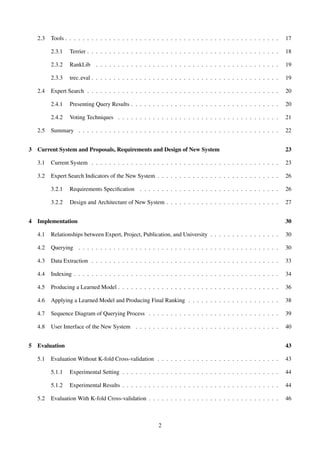
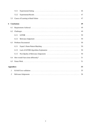
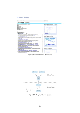
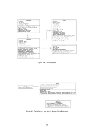
This document describes a project to develop an expert search system that mines academic expertise from funded research in Scottish universities. The system aims to integrate data on funded projects from external sources with an existing academic search engine to improve its search results. It will extract expertise information from publications and funded projects to generate expert profiles. Learning to rank algorithms will then be used to rank experts based on their profiles for specific queries. The goal is to enhance the current search engine that identifies experts based on publications by incorporating additional evidence of expertise from funded research projects.


![Chapter 1
Introduction
This chapter is about the introduction of the project. It will give an overview of The Scottish Informatics and
Computer Science Alliance (SICSA), the existing search engine, definition of the project and aims. It will also
outline the structure of the project.
1.1 The Scottish Informatics and Computer Science Alliance (SICSA)
“The Scottish Informatics and Computer Science Alliance (SICSA) is a collaboration of Scottish Universities
whose goal is to develop and extend Scotland’s position as a world leader in Informatics and Computer Science
research and education” [13]. SICSA achieves this by working cooperatively rather than competitively, by pro-
viding support and sharing facilities, by working closely with industry and government and by appointing and
retaining world-class staff and research students in Scottish Universities. A list of members of SICSA is given in
table 1.1.
1.2 What is Expert Search?
With the enormous in the number of information and documents and the need to access information in large
enterprise organisations, “collaborative users regularly have the need to find not only documents, but also people
with whom they share common interests, or who have specific knowledge in a required area” [26, P. 388]. In
an expert search task, the users’ need, expressed as queries, is to identify people who have relevant expertise to
the need [26, P. 387]. An expert search system is an Information Retrieval [2] system that makes use of textual
evidence of expertise to rank candidates and can aid users with their “expertise need”. Effectively, an expert
University
University of Aberdeen
University of Abertay
University of Dundee
University of Edinburgh
Edinburgh Napier University
University of Glasgow
Glasgow Caledonian University
Heriot-Watt University
Robert Gordon University
University of St Andrews
University of Stirling
University of Strathclyde
University of the West of Scotland
Table 1.1: A list of members of SICSA
4](https://image.slidesharecdn.com/4fde60ad-44a6-4bcf-8ac2-2d1594a4aa54-160724173420/85/dissertation-7-320.jpg)
![search systems work by generating a “profile” of textual evidence for each candidate [26, P. 388]. The profiles
represent the system’s knowledge of the expertise of each candidate, and they are ranked in response to a user
query [26, P. 388]. In real world scenario, the user formulates a query to represent their topic of interest to the
system; the system then uses the available textual evidence of expertise to rank candidate persons with respect to
their predicted expertise about the query.
1.3 Definition of Mining Academic Expertise from Funded Research and Aims
http://experts.sicsa.ac.uk/ [12] is a deployed academic search engine that assists in identifying the relevant ex-
perts within Scottish Universities, based on their recent publication output. However, integrating different kinds
of academic expertise evidence with the existing one may improve the effectiveness of the retrieval system. The
aim of this project is to develop mining tools for the funded projects, and research ways to integrate them with
the existing academic search engines to obtain the most effective search results. The sources of the new evidence,
funded projects, are from Grant on the Web [1] and Research Councils UK [11]. To integrate academic funded
projects and publications together, Learning to Rank Algorithms for Information Retrieval (IR) are applied in
this project.
1.4 Context
This project was initially developed by an undergraduate student a few years ago. It used academic’s publications
as an expertise evidence to find experts. I have access to funded projects data in the UK. This data is integrated
with existing data to improve the effectiveness of http://experts.sicsa.ac.uk/ [12] at answering expert search
queries. The internal name of the codebase is AcademTech. Some chapters might use this name.
1.5 Overview
In this dissertation, section 2 aims to explain the backgrounds of the project to readers. Section 3 includes
discussions of system and interface designs and architecture and proposals to the new system. This section is
necessary for readers to understand other sections. Section 4 discusses about implementations of the system and
new system user interface design. Section 5 provides results and analysis of the techniques used. This section
can be viewed as the most important part of the whole project since it analyses whether applying a learning to
rank technique improves the effectiveness of the system or not. The last section is the conclusions of the project.
5](https://image.slidesharecdn.com/4fde60ad-44a6-4bcf-8ac2-2d1594a4aa54-160724173420/85/dissertation-8-320.jpg)
![Chapter 2
Background
This chapter is aimed to give backgrounds required to understand the rest of the chapters. It begins with In-
formation Retrieval (IR) and Search Engine (Section 2.1). Then Section 2.2 will dicuss about Learning to Rank
(LETOR) In Information Retrieval. Tools used in this project will be briefly discussed in Section 2.3. And finally,
Section 2.4 will discuss expert search and techniques related to it in more details.
2.1 Information Retrieval (IR) and Search Engine
“Information Retrieval (IR) is the activity of obtaining information resources relevant to an information need
from a collection of information resources” [2]. An information retrieval process begins when a user enters a
query into the system. Queries are formal statements of information needs, for example search strings in web
search engines. However, the submitted query may not give the satisfying results for the user. In this case, the
process begins again. Figure 2.1 illustrates search process. As information resources were not originally intended
for access (Retrieval of unstructured data)[P. 7] [29], it is impossible for a user query to uniquely identify a single
object in the collection. Instead, several objects may match the query, with different degrees of relevancy. In
the IR field, there are various types of retrieval models used to compute the degree of relevancy. This will be
discussed in more details in Section 2.1.2.
A search engine is an information retrieval system designed to help find information stored on a computer
system [22]. The search results are usually presented in a list ordered by the degree of relevancy and are com-
monly called hits. Search engines help to minimize the time required to find information and the amount of
information which must be consulted [22]. The special kind of search engine is web search engine. It is a soft-
ware system that is designed to search for information on the World Wide Web [25] such as Google, Bing, and
Yahoo.
2.1.1 Brief Overview of Information Retrieval System Architecture
In IR systems, two main objectives have to be met [28] - first, the results must satisfy user - this means retrieving
information to meet user’s information need. The second, retrieving process must be fast. This section is devoted
to a brief overview of the architecture of IR systems which is very important to meet the IR main objectives. It
also explains readers how documents are retrieved and the data structure used in IR systems. To understand how
retrieval process works, we must understand indexing process first. This process is performed offline and only
one time. There are 4 steps involved in indexing process and each process is performed sequentially [28]:
6](https://image.slidesharecdn.com/4fde60ad-44a6-4bcf-8ac2-2d1594a4aa54-160724173420/85/dissertation-9-320.jpg)

![Term frequency
two 1
ways 1
live 1
life 1
one 1
nothing 1
miracle 2
everything 1
Table 2.2: Terms and Frequency After Stopwords Removal
Term frequency
two 1
way 1
live 1
life 1
one 1
nothing 1
miracle 2
everything 1
Table 2.3: Terms and Frequency After Stemming
Table 2.1 shows all the terms and frequency of each term in the document. It can be seen that there are some
words in the document which occur too frequently. These words are not good discriminators. They are referred
to as “stopwords”. Stopwords include articles, prepositions, and conjunctions etc.
Tokenisation is the process of breaking a stream of text into words called tokens(terms) [24]. The stream of
text will be used by other indexing steps.
Stopwords Removal is the process of removing stopwords in order to reduce the size of the indexing struc-
ture [28, P. 15]. Table 2.2 shows all the terms and frequency of each term after stopwords removal process.
Stemming is the process of reducing all words obtained with the same root into a single root [28, P. 20]. A
stem is the portion of a word which is left after the removal of its affixes (i.e. prefixes and suffixes). For example,
connect is the stem for the variants connected, connecting, and connection. This process makes the size of the
data shorter. There are various stemming algorithms such as Porter Stemming, and Suffix-stripping algorithms.
After stemming, all terms in the table are in its root forms. If a document is large in size, this process can
reduce the size of the data considerably. However, there is one drawback. That is, it prevents interpretation
of word meanings. For instance, the root form of the term “gravitation” is “gravity”. But the meaning of
“gravitation” is different from “gravity”.
Figure 2.3: Simple Inverted Index
8](https://image.slidesharecdn.com/4fde60ad-44a6-4bcf-8ac2-2d1594a4aa54-160724173420/85/dissertation-11-320.jpg)
![Inverted Index Structure Creation is the process that creates an index data structure storing a mapping from
terms(keys) to its locations in a database file, or in a document or a set of documents(values) [18]. The purpose
of this data structure is to allow a full text searches. In IR, a value in a key-value pair is called posting. There are
a number of index structures used in practice. However, the index used in most IR systems and in this project is
inverted index. Figure 2.3 shows a simple inverted index. Given a query (a set of terms), it is now possible to effi-
ciently search for documents containing those terms. However, each posting may contain additional information
or features about a document such as the frequency of the term etc.
2.1.2 Retrieval Models
In the previous section, basic indexing process was briefly explained. In this section, we will give a brief introduc-
tion to a few retrieval models including one used in this project. In general, retrieval models can be categorised
into 2 categories: probabilistic approach and non probabilistic approach. This section will briefly explain Term
Frequency–Inverse Document Frequency (tf-idf), BM25 and PL2 retrieval models.
Term Frequency–Inverse Document Frequency (tf-idf)
tf-idf is a numerical statistic that is intended to reflect how important a word is to a document in a collec-
tion [23]. As the name suggests, it consists of 2 parts: term frequency (tf) and inverse document frequency (idf).
Term frequency is the number of occurrences a term appears in a document. Inverse document frequency (idf) is
a measure of whether the term is common or rare across all documents [23]. This component is very important
for instance, if a query term appears in most of the documents in the corpus, it is not appropriate to give a doc-
ument containing that term a high score because that term is not a very good discriminator. On the other hand,
it is appropriate to give high scores to documents containing terms rarely appear in the corpus. The following is
the formula of tf-idf weighting model:
Wfk = ffdlog
N + 1
Dk + 1
(2.1)
where N is the number of documents in the collection, ffd is tf of kth keyword in document d (term frequency),
and Dk is the number of documents containing kth keyword. The log N+1
Dk+1 is the idf of the model. The numerator
and denominator are added by 1 to prevent possibility of zero. This model is a non-probabilistic approach and is
one of the easiest to implement models in IR.
BM25
BM25 is a very popular probabilistic retrieval model in IR. Why use probabilities? In Section 2.1, we explained
that IR deals with uncertain and unstructured information. In other words, we do not know specifically what
the documents are really about. As a consequence, a query does not uniquely identify a single object in the
collection. Therefore, probability theory seems to be the most natural way to quantify uncertainty [31, P. 7].
Based on a derivation from the probabilistic theory, the formula for BM25 is shown below:
score(d, q) =
t∈q
log2
rt/(R − rt)
(nt − rt)/(N − nt − R + rt)
(k1 + 1) · tftd
K + tftd
k2 + 1) · tftq
k2 + tftq
(2.2)
where K = kt((1−b)+b dl
avdl ), tftq and tftd are the frequency of term t in the query q and document d respectively,
and b, dl and avdl are parameters set empirically. rt is the number of documents containing term t relevant to
a query term t. R is the number of documents in the collection relevant to a query term t. nt is the number of
documents in which the query term t appears and N is the number of all documents in the collection. The proof
of BM25 is beyond the scope of the project.
9](https://image.slidesharecdn.com/4fde60ad-44a6-4bcf-8ac2-2d1594a4aa54-160724173420/85/dissertation-12-320.jpg)
![Figure 2.4: Retrieval Process
PL2
PL2 is a model from the divergence from randomness framework, based on a poisson distribution [19]. This
project uses PL2 weighting model to calculate document scores. This model is also a probabilistic approach.
Given a document d and a query q, the formula of PL2 [34, P. 23-24] is given below:
score(d, q) =
t∈q
qtw ·
1
tfn + 1
(tfn · log2
tfn
λ
+ (λ − tfn) · log2e + 0.5 · log2(2π · tfn)) (2.3)
where λ is the mean and variance of a Poisson distribution, and the query weight term qtw is given by qtf/qtfmax.
qtf is the query term frequency. qtfmax is the maximum query term frequency among the query terms. From
equation 2.3,
tfn = tf · log2(1 + c ·
avgl
l
), c > 0
where tf is the actual term frequency of the term t in document d and l is the length of the document in tokens.
avgl is the average document length in the whole collection. c is the hyper-parameter that controls the normali-
sation applied to the term frequency with respect to the document length. The proof and explanation are out of
the scope of the project.
2.1.3 Retrieval Process in Information Retrieval
Section 2.1.1 and Section 2.1.2 explained basic indexing process and a few retrieval models respectively. In this
section, we will see how documents are retrieved. Figure 2.4 shows retrieval process of IR system. In IR, there
are 2 phases in general: online and offline phases. The offline phase is the phase that all documents in the corpus
are indexed, all features are extracted and index structure is built (Section 2.1.1).
On the other hand, online phase begins after a user submits a query into the system. After that, tokenisation,
stopwords removal and stemming processes are performed as same as the offline phase. Features can also be
extracted from query terms as well. At this point, it comes to the process of matching and assigning scores to
documents. This process can make use of one of the retrieval models explained in Section 2.1.2. In this project,
PL2 weighting model and voting technique which will be explained in Section 2.4.2 are used to compute scores.
Once scores have been assigned to relevant documents, the system ranks all documents in order of decreasing
scores and show to the user. Figure 2.4 gives a graphical representation of retrieval process.
10](https://image.slidesharecdn.com/4fde60ad-44a6-4bcf-8ac2-2d1594a4aa54-160724173420/85/dissertation-13-320.jpg)
![2.1.4 Evaluation
This section is devoted to backgrounds of evaluation of IR systems. It is very important as it is a background for
Evaluation Chapter. Since IR is research-based, understanding how evaluation is carried out will enable readers
to determine whether this project is achieved or not. There are 3 main reasons for evaluating IR systems [30, P.
3]:
1. Economic reasons: If people are going to buy the technology, they want to know how effective it is.
2. Scientific reasons: Researchers want to know if progress is being made. So they need a measure for
progress. This can show that their IR system is better or worse than someone else’s.
3. Verification: If an IR system is built, it is necessary to verify the performance.
To measure information retrieval effectiveness in the standard way, a test collection is required and it consists
of 3 things [17]:
1. A document collection.
2. A test suite of information needs, expressible as queries.
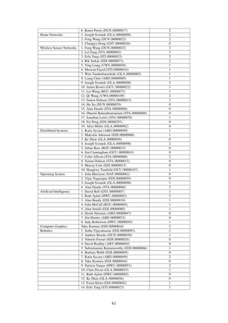
3. A set of relevance judgments, usually a binary assessment of either relevant or nonrelevant for each query-
document pair.
The standard approach to information retrieval system evaluation revolves around the notion of relevant and
nonrelevant documents. With respect to a user’s information need, a document in the test collection is given a
binary classification as either relevant or nonrelevant [17]. However, this can be extended by using numbers as an
indicator of the degree of relevancy called graded relevance value. For example, documents labelled 2 is more
relevant than documents labelled 1, and documents labelled 0 is not relevant. In IR, a binary classification as
either relevant or nonrelevant and graded relevance value are called relevance judgement. There are a number
of test collection standards. In this project, Text Retrieval Conference (TREC) [15] is used since it is widely used
in the field of IR.
Precision and Recall
The function of an IR system is to [30, P. 10]:
• retrieve all relevant documents measured by Recall
• retrieve no non-relevant documents measured by Precision
Precision (P) is the fraction of retrieved documents that are relevant
Recall (R) is the fraction of relevant documents that are retrieved
11](https://image.slidesharecdn.com/4fde60ad-44a6-4bcf-8ac2-2d1594a4aa54-160724173420/85/dissertation-14-320.jpg)
![Figure 2.5: Precision-Recall Graph
If a system has high precision but low recall, the system returns relevant documents but misses many useful
ones. If a system has low precision but high recall, the system returns most relevant documents but includes lots
of junks. Therefore, the ideal is to have both high precision and recall. To give a good example, consider Figure
2.5, since overall IR system A (blue) has higher precision than IR system B (red), system A is better than system
B.
In this project, 3 evaluation metrics are chosen: Mean Average Precision (MAP), Normalized Discounted
Cumulative Gain (NDCG) and Mean Reciprocal Rank (MRR). Each of them has different behaviours.
Mean Average Precision (MAP)
MAP for a set of queries is the mean of the average precision scores for each query [2]. The equation below is a
formula for MAP.
where Q is the number of queries.
Mean Reciprocal Rank (MRR)
MRR is a statistic measure for evaluating a list of possible responses to a set of queries, ordered by probability
of correctness [21]. The equation below is a formula for MRR.
where ranki is the position of the correct result and Q is the number of queries.
12](https://image.slidesharecdn.com/4fde60ad-44a6-4bcf-8ac2-2d1594a4aa54-160724173420/85/dissertation-15-320.jpg)
![Normalized Discounted Cumulative Gain (NDCG or nDCG)
To understand NDCG, first of all, we have to understand Discounted Cumulative Gain (DCG). The premise
of DCG is that highly relevant documents appearing in lower position in a search result list should be penalized
as the graded relevance value (discussed above) is reduced logarithmically proportional to the position of the
result. [20]. The discounted CG accumulated at a particular rank position p is defined as:
where reli is the graded relevance value of the result at position i.
From DCG, we can formulate NDCG as follows:
where IDCGp is the maximum possible (ideal) DCG for a given set of queries, documents, and relevances.
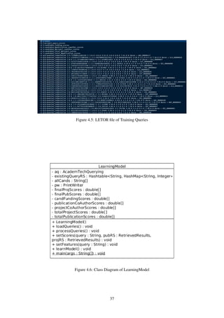
2.2 Learning to Rank (LETOR) In Information Retrieval
Learning to rank or machine-learned ranking (MLR) is a type of supervised or semi-supervised machine learning
problem in which the goal is to automatically construct a ranking model from training data [35]. Employing
learning to rank techniques to learn the ranking function is important as it is viewed as a promising approach
to information retrieval [35]. In particular, many learning to rank approaches attempt to learn a combination of
features (called the learned model) [27, P. 3]. The resulting learned model is applied to a vector of features for
each document, to determine the final scores for producing the final ranking of documents for a query [27, P.
3]. In LETOR, there are typically 2 types of dataset: training and testing dataset. They both consist of queries
and documents matching them together with relevance degree of each match [4] and are typically prepared
manually by human assessors, who check results for some queries and determine relevance of each result or
derived automatically by analyzing clickthrough logs (i.e. search results which got clicks from users). However,
they differ in the purpose of usage.
• Training data is used by a learning algorithm to produce a ranking model or learned model [4]. This will
discuss in more details in Section 2.2.5
• Testing data is applied with a learned model and used to evaluate the effectiveness of the system [19].
2.2.1 Query Dependent Feature
Figure 2.1 shows a simple search process in IR. After a user submits a query into an IR system, the system ranks
the documents with respect to the query in descending order of the documents’ scores and returns a documents
set to the user. It can be clearly seen that the documents obtained with respect to the query depends on the query
the user submitted. In other words, document A can have 2 different degrees of relevancy if a user changes
a query. In learning to rank, this is called query dependent feature [19]. To give a good example, consider
an IR system using tf-idf retrieval model (see Section 2.1.2). From equation 2.1, given a document d, query
13](https://image.slidesharecdn.com/4fde60ad-44a6-4bcf-8ac2-2d1594a4aa54-160724173420/85/dissertation-16-320.jpg)
![q = {database}, fdatabase,d = 5, N = 120, and Ddatabase = 23, the score of document d is 3.51. If a query is
changed to q = {information}, then the score of document d is possibly different depending on the parameters
in the formula.
2.2.2 Query Independent Feature
In contrast to Query Dependent Feature, a feature that does not depend on a user query is called query inde-
pendent feature [19]. This feature is fixed for each document. To give a good example, consider an algorithm
used by Google Search to rank websites in their search engine results. This algorithm is called PageRank [6].
According to Google, how PageRank works is given below [6]:
PageRank works by counting the number and quality of links to a page to determine a rough
estimate of how important the website is. The underlying assumption is that more important websites
are likely to receive more links from other websites.
In IR, the link of a website is actually a document. It is obvious that PageRank takes query independent
features into account which are number of links and quality of links to a website.
2.2.3 Learning to Rank File Format
From the previous 2 sections, we now know what query dependent and query independent features are. In this
section, we will talk about how these features are formatted in a file called LETOR file. The LETOR file is then
learned to obtain a model file (see next section). The following is the format of LETOR file:
#feature num1:feature name1
#feature num2:feature name2
graded relevance value qid:query feature num1:feature name1 score feature num2:feature name2 score
#docno = document id
In this LETOR file, there are 2 features, feature name1 and feature name2. In LETOR file, items after a hash
symbol are ignored. The lines not preceded by hash symbol are learned. They represent documents with scores
of each feature. graded relevance value is a label which indicates the degree of relevancy (see last section). If
the label is 0, it means the document is irrelevant with respect to a query. If it is 1, the document is relevant.
In this project, graded relevance value ranges from 0 to 2 in order of the degree of relevancy. To the left of the
label is a query preceded by qid : and scores of each feature associated to a document. There can be any number
of documents in the LETOR file. The example of a real LETOR file is given below:
#1:publicationQuery
#2:projectQuery
2 qid:Information Retrieval 1:3.4 2:1.1 #docno = GLA 000001
In this example, there are 2 features: publicationQuery and projectQuery. The document GLA 000001 with
respect to the query InformationRetrieval is perfectly relevant with graded relevance value of 2. It has 2
feature values for publicationQuery and projectQuery which are 3.4 and 1.1 respectively.
14](https://image.slidesharecdn.com/4fde60ad-44a6-4bcf-8ac2-2d1594a4aa54-160724173420/85/dissertation-17-320.jpg)
![2.2.4 Learning to Rank Model File Format
After a LETOR file is learned, we obtain a Learned Model. This section aims to show some learned model file
formats.
## Coordinate Ascent
## Restart = 2
## MaxIteration = 25
## StepBase = 0.05
## StepScale = 2.0
## Tolerance = 0.001
## Regularized = false
## Slack = 0.001
1:0.64 2:4.34 3:4.3 4:2.0 5:1.2 6:9.1 7:3.3
The lines preceded by hash symbols are ignored. The above learned model applies Coordinate Ascent LETOR
technique. Knowing what parameters preceded by hash symbols mean is out of the scope of the project. We
only take lines not preceded by hash symbols into account. According to the above learned model, there are 7
features (1 to 7). The floating values associated to each feature indicate a score of the feature. However, some
LETOR algorithms might produce duplicate features such as 1:0.64 2:4.34 3:4.3 4:2.0 5:1.2 6:9.1 7:3.3 1:1.2
5:3.2. In this case, we sum up values corresponding to the feature, giving 1:1.84 2:4.34 3:4.3 4:2.0 5:4.4 6:9.1
7:3.3. AdaRank is one of those algorithms.
2.2.5 Obtaining and Deploying a Learned Model
The general steps for obtaining a learned model using a learning to rank technique are the following [27, P. 4]:
1. Top k Retrieval: For a set of training queries, generate a sample of k documents using an initial
retrieval approach.
2. Feature Extraction: For each document in the sample, extract a vector of feature values.
3. Learning: Learn a model by applying a learning to rank technique. Each technique deploys a
different loss function to estimate the goodness of various combination of features. Documents are
labelled according to available relevance assessments.
Once a learned model has been obtained from the above learning steps, it can be deployed within a
search engine as follows [27, P. 4]
4. Top k Retrieval: For an unseen test query, a sample of k documents is generated in the same
manner as step (1).
5. Feature Extraction: As in step (2), a vector of feature values is extracted for each document in
the sample. The set of features should be exactly the same as for (2).
6. Learned Model Application: The final ranking of documents for the query is obtained by applying
the learned model on every document in the sample, and sorting by descending predicted score.
Figure 2.6 illustrates an architecture of a machine-learned IR system. How this architecture links to our
approach will be discussed in Section 4.
15](https://image.slidesharecdn.com/4fde60ad-44a6-4bcf-8ac2-2d1594a4aa54-160724173420/85/dissertation-18-320.jpg)
![Figure 2.6: An architecture of a machine-learned IR system from http://en.wikipedia.org/wiki/
Learning_to_rank
2.2.6 Applying a Learned Model
Once a learned model has been generated, then for each document retrieved after retrieval, the scores of each
feature are multiplied by ones in the learned model and accumulated. Finally, the accumulated scores for each
document are sorted in descending order and documents with the high scores are ranked before those with low
scores.
2.2.7 Learning to Rank Algorithms
In this project, we use only 2 LETOR algorithms which are AdaRank [33, P. 60] and Coordinate Ascent [36]. Full
detailed explanations of the algorithms are out of the scope of this project. The algorithms are chosen because of
its simplicity and its effectiveness.
Coordinate Ascent
Coordinate Ascent Algorithm is an adaptation of Automatic Feature Selection Algorithm [36]. It is also a linear
model [38, P. 1-4] based LETOR algorithm as same as AdaRank.
Let Mt denote the model learned after iteration t. Features are denoted by f and the weight (parameter)
associated with feature f is denoted by λf . The candidate set of features is denoted by F. A model is represented
as set of pairs of feature/weight. We assume that SCORE(M) returns the goodness of model M with respect to
some training data.
The algorithm shown in Figure 2.7 starts with an empty model Mt. The feature f is added to the model. AFS
is used to obtain the best λf . The utility of feature f (SCOREf ) is defined to be the maximum utility obtained
during training. This process is repeated for every f ∈ F. The feature with maximum utility is then added to the
model and removed from F. The entire process is then repeated until the change in utility between consecutive
iterations drops.
16](https://image.slidesharecdn.com/4fde60ad-44a6-4bcf-8ac2-2d1594a4aa54-160724173420/85/dissertation-19-320.jpg)
![begin
t := 0
Mt :={}
while SCORE(Mt) − SCORE(Mt−1) > 0 do
for f ∈ F do
ˆλ := argmaxλf
SCORE(M ∪ {(f, λf )}) AFS is used to obtain λf
SCOREf := SCORE(M ∪ {(f, ˆλf )})
end
f∗ := argmaxf SCOREf
M := M ∪ {(f∗, ˆλf∗ )}
F := F − {f∗}
t := t + 1
end
end
Figure 2.7: Pseudocode of Coordinate Ascent
AdaRank
AdaRank is a linear model [38, P. 1-4] based LETOR algorithm. It repeats the process of reweighting the training
data, creating a weak ranker, and assigning a weight to the weak ranker, to minimise the loss function [33, P.
60]. In this project, a loss function is an evaluation measure such as MAP, NDCG, etc. Then AdaRank linearly
combines the weak rankers as the ranking model. One advantage of AdaRank is its simplicity, and it is one of
the simplest learning to rank algorithms [33, P. 60]. In Section 2.2.4, we discussed that AdaRank is one of the
LETOR algorithms which produce duplicate features such as 1:0.64 2:4.34 3:4.3 4:2.0 5:1.2 6:9.1 7:3.3 1:1.2
5:3.2. The reason behind it is that AdaRank can select the same feature multiple times [19].
2.2.8 K-fold Cross-validation
In Sections 2.2 and 2.2.5, we talked about 2 mandatory types of data: training and testing data. If our learned
model is based too much on training data (pays too much attentions on training data), the predictions for unseen
testing data are very poor. This is often the case, when our training dataset is very small [38]. In machine
learning, we call it over-fitting [38, P. 28]. Determining the optimal model such that it is able to generalise well
without over-fitting is very challenging. This is why we need validation data. A validation data is typically
provided separately or removed from original dataset [19]. K-fold cross-validation splits the original dataset into
K equally sized blocks or folds [38]. Each fold takes its turn as a validation data for a training data comprised of
the other K - 1 folds [38]. Figure 2.8 describes K-fold Cross-validation graphically.
2.3 Tools
This section will discussed tools used in this project. They include search engine platform Terrier, learning to
rank library RankLib and evaluation tool, trec eval.
17](https://image.slidesharecdn.com/4fde60ad-44a6-4bcf-8ac2-2d1594a4aa54-160724173420/85/dissertation-20-320.jpg)
![Figure 2.8: K-fold Cross-validation from Machine Learning Lecture 3 - Linear Modelling By Simon Rogers
Figure 2.9: Indexing Architecture of Terrier from http://terrier.org/docs/v3.5/
basicComponents.html
2.3.1 Terrier
Every IR system requires programs that handle indexing, retrieving, ranking, etc. To build everything from
scratch, it would be impossible within the 1 year duration. However, there are a number of search engine
platforms that deal with IR functionalities effectively. Terrier [14] was chosen because it is a highly flexible,
efficient, and effective open source search engine. It is a comprehensive, and flexible platform for research and
experimentation in text retrieval. Research can easily be carried out on standard TREC collection [15]. Using
Terrier, this project can easily extend from the existing search engine as it used Terrier as a search engine platform
and it is written in Java which is the same programming language used in this project.
Terrier Indexing
Figure 2.9 gives an overview of the interaction of the main components involved in the indexing process of
Terrier.
1. A corpus will be represented in the form of a Collection object. Raw text data will be repre-
sented in the form of a Document object. Document implementations usually are provided with an
instance of a Tokeniser class that breaks pieces of text into single indexing tokens.
18](https://image.slidesharecdn.com/4fde60ad-44a6-4bcf-8ac2-2d1594a4aa54-160724173420/85/dissertation-21-320.jpg)
![2. The indexer is responsible for managing the indexing process. It iterates through the docu-
ments of the collection and sends each found term through a TermPipeline component.
3. A TermPipeline can transform terms or remove terms that should not be indexed. An example
for a TermPipeline chain is termpipelines=Stopwords,PorterStemmer, which removes terms from the
document using the Stopwords object, and then applies Porter’s Stemming algorithm for English to
the terms.
4. Once terms have been processed through the TermPipeline, they are aggregated and the
following data structures are created by their corresponding DocumentBuilders: DirectIndex, Doc-
umentIndex, Lexicon, and InvertedIndex.
5. For single-pass indexing, the structures are written in a different order. Inverted file postings
are built in memory, and committed to ’runs’ when memory is exhausted. Once the collection had
been indexed, all runs are merged to form the inverted index and the lexicon.
2.3.2 RankLib
RankLib [9] is an open source library of learning to rank algorithms. It provides various retrieval metrics to
facilitate evaluation. Currently 8 popular algorithms have been implemented:
• MART (Multiple Additive Regression Trees, a.k.a. Gradient boosted regression tree)
• RankNet
• RankBoost
• AdaRank
• Coordinate Ascent
• LambdaMART
• ListNet
• Random Forests
This library was chosen because it is easy to use, written in Java which can be easily combined with this
system as it is also developed using Java, and it implements 8 different learning to rank algorithms which makes
it possible for users to try different algorithms. However, AdaRank and Coordinate Ascent were only used in
the project because other algorithms are too complex and not part of the scope of this project. RankLib provides
k-fold cross validation functionality given only training dataset. This saves us time to split data for validation,
training and testing as described in Section 2.2.
2.3.3 trec eval
trec eval is the standard tool used by the TREC community [15] for evaluating a retrieval run, given the results
file and a standard set of judged results. trec eval was chosen because the data used in this project uses TREC
format. It is easy to use and written in C which makes the tool efficient. To use trec eval, 2 files are required:
qrels and result file in TREC format. qrels is a file that stores relevant results for queries stored in a queries
file [8]. It has the following format [10]:
TOPIC ITERATION DOCUMENT# RELEVANCY
19](https://image.slidesharecdn.com/4fde60ad-44a6-4bcf-8ac2-2d1594a4aa54-160724173420/85/dissertation-22-320.jpg)
![where TOPIC is the query, ITERATION is the feedback iteration (almost always zero and not used), DOCU-
MENT# is the official document number that corresponds to the ”docno” field in the documents (in this project,
expert’s id), and RELEVANCY is a number indicating a degree of relevancy. In this project, 3 numbers: 0, 1,
and 2 indicating non-relevant, relevant and perfectly relevant respectively, are used. The result file is the file that
contains the following [16]:
TOPIC ITERATION DOCUMENT# RANK SIM RUN ID
where RANK is the position of the corresponding document# in a ranking, SIM is a float value indicating a score
and RUN ID is a string which gets printed out with the output.
After trec eval is run, it will give measures of metrics discussed in Section 2.1.4. To obtain NDCG measure,
trec eval requires an additional argument (-m ndcg) when it is run.
2.4 Expert Search
In Section 1.2, we discussed about the definition of Expert Search. This section will give 5 scenarios proposed by
Yimam-Seid & Kobsa why expert search is needed [26, P. 387] and outline several ways to present query results.
1. Access to non-documented information - e.g. in an organisation where not all relevant infor-
mation is documented.
2. Specification need - the user is unable to formulate a plan to solve a problem, and resorts to
seeking experts to assist them in formulating a plan.
3. Leveraging on another’s expertise (group efficiency) - e.g. finding a piece of information that
a relevant expert would know/find with less effort than the seeker.
4. Interpretation need - e.g. deriving the implications of, or understanding, a piece of informa-
tion.
5. Socialisation need - the user may prefer that the human dimension be involved, as opposed to
interacting with documents and computers.
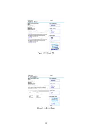
2.4.1 Presenting Query Results
Figure 2.1 illustrates the process of search. From this figure, the process will start again if a user is not satisfied
with the results. In this section, the focus is on how to convince user that a query result is good. Suppose a user
who is currently studying software engineering would like to know “how to normalise database tables”, first of
all, he needs to interpret his information need into a query which is “database normalisation”. He then types his
query into his preferred search engine. After he submits the query, the search engine gives him a list of results
ranked by the degree of relevancy. The question is how does he determine which result is what he is looking
for?. Well, he could assume that the ranking provided by the search engine is correct. That is, the first result is
what he is looking for. However, this is not always the case. He then explores each result and sees if it is the
right one. But without exploring each result, could he be able to determine that which result is likely to satisfy
his information need? Perhaps, there has to be some evidence to convince him by just looking at the result. The
followings are evidence he could take into account [19]:
• URL
20](https://image.slidesharecdn.com/4fde60ad-44a6-4bcf-8ac2-2d1594a4aa54-160724173420/85/dissertation-23-320.jpg)
![Figure 2.10: Sample Query
• Photo
• Author’s Name
• keywords of the article name
If a result in response to a query has all or some of these evidence, it has more credits than ones with no evidence
at all. Figure 2.10 shows the results of the query “database normalisation”. It is obvious that from the top 4
results, all of the article names include the keywords a user submitted, and the third result does not have query
keywords included in the URL. Among all of which, the second result has more evidence than others. It has an
author’s name, a photo of an author that other results do not. In this project, these evidence of credits also take
into account. However, we are unable to take photo into account because the datasource (see Section 1.3) does
not provide photos of experts.
2.4.2 Voting Techniques
In Section 2.1.3, we very briefly talked about weighting models or retrieval models. In other words, how
documents are assigned scores. In expert search, we rank experts (people), not documents directly. In this
section, it aims to give an overview of a voting technique used in this project. To understand this section, readers
must understand what data fusion technique is. “Data fusion techniques also known as metasearch techniques,
are used to combine separate rankings of documents into a single ranking, with the aim of improving over the
performance of any constituent ranking” [26, P. 388]. Within the context of this project, expert search is seen
as a voting problem. The profile of each candidate is a set of documents associated to him to represent their
expertise. When each document associated to a candidate’s profile get retrieved by the IR system, implicit vote
for that candidate occurs [26, P. 389]. Data fusion technique is then used to combine the ranking with respect
to the query and the implicit vote. In expert search task, it shows that “improving the quality of the underlying
document representation can significantly improve the retrieval performance of the data fusion techniques on
an expert search task” [26, P. 387]. To give a simple example how voting technique works, take a look at this
example
Let R(Q) be the set of documents retrieved for query Q, and the set of documents belonging to the profile
candidate C be denoted profile(C). In expert search, we need to find a ranking of candidates, given R(Q).
21](https://image.slidesharecdn.com/4fde60ad-44a6-4bcf-8ac2-2d1594a4aa54-160724173420/85/dissertation-24-320.jpg)


![The requirements have been split into 2 sections depending on their necessity: functional requirements and
non-functional requirements
Functional Requirements
Must Have
• Extracting funded projects from 2 different sources: Grant on the Web [1] and Research Councils UK [11].
• Integrating publications and funded projects as expertise evidence.
• Utilizing learning to rank techniques with an attempt to improve the effectiveness of the retrieval system
using AdaRank and Coordinate Ascent algorithms.
Should Have
• Refinement options for users to filter results by funded projects, publications and both.
• Refinement options for users to filter funded projects and publications of each expert.
Could Have
• Applications of more LETOR algorithms such as LambdaMART, Random Forests etc.
Would Like to Have
• Ability to upload funded projects manually by members of the system.
Non-functional Requirements
• Functional 24 hours a day.
• Update data regularly.
• Able to load all evidence into main memory for efficient lookup.
• Fully functional for the purpose of the final demonstration.
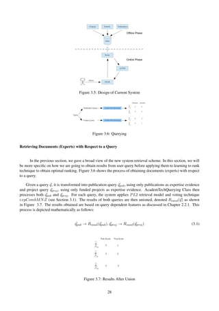
3.2.2 Design and Architecture of New System
Figure 3.5 shows design of the new system. It makes use of learning to rank (LETOR) technique to integrate
both publications and funded projects as expertise evidence. From the figure, in contrast to the current system,
LETOR is applied to documents retrieved from Terrier. This LETOR reranks the documents to get the optimal
ranking.
27](https://image.slidesharecdn.com/4fde60ad-44a6-4bcf-8ac2-2d1594a4aa54-160724173420/85/dissertation-30-320.jpg)
![Figure 4.4: Projects Extraction Class Diagrams
4.3 Data Extraction
In Chapter 1.3, it was stated that funded projects are obtained from Grant on the Web [1] and Research Coun-
cils UK [11]. This section shows classes used to extract funded projects from each source and gives statistics
regarding the number of funded projects from each source. Figure 4.4 shows a class diagram related to projects
extraction task.
• AcademicsHashTable is an abstract class which makes use of HashMap data structure,
Map < Character, LinkedList < Candidate >>, for efficient look up when matching candidate to
our known candidates. It is keyed by the first character of candidate’s name. There are 2 abstract methods
in this class: has() and checkAcademicName() methods. Both of them are used together to check if the
candidate is matched to our known candidates.
• GtRHashTable extends from the abstract class AcademicsHashTable. The purpose of this class is the
same as AcademicsHashTable Class but implements has() and checkAcademicName() methods which are
applicable in Research Councils UK [11] data source.
• GOWHashTable extends from the abstract class AcademicsHashTable. Its purpose is similar to Aca-
demicsHashTable Class but has different implementations of has() and checkAcademicName() methods to
GOWHashTable’s which are applicable in Grant on the Web [1] spreadsheet data source.
• SSProjectsExtractor is a class that makes use of GOWHashTable Class to extract funded projects from
Grant on the Web [1] spreadsheet.
• GtRProjectWrapper is a class used GOWHashTable Class to extract funded projects from Research
Councils UK [11].
• ProjectExtractor is a class that makes use of SSProjectsExtractor and GtRProjectWrapper Classes to
extract funded projects from both sources.
Since each source records expert’s name in different formats. For example, Prof. Joemon Jose may be
recorded Jose JM in one source and Jose J in another, Polymorphism [7] (in this case, different implementations
33](https://image.slidesharecdn.com/4fde60ad-44a6-4bcf-8ac2-2d1594a4aa54-160724173420/85/dissertation-36-320.jpg)
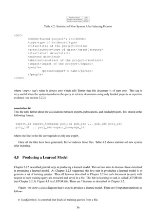
![Source Number of Funded Projects
Grant on the Web 32
Research Councils UK 337
369 total
Table 4.1: The number of funded projects extracted from each source
of has() and checkAcademicName() methods between GtRHashTable and GOWHashTable) is required. How-
ever, pattern matching between expert’s names in Grant on the Web [1] spreadsheet is still impossible as this
source records in the following format: [lastname], [role] [the first and/or second letter of name] such as Rogers,
Dr. Simon. The problem occurs with experts, Dr. Craig Macdonald lecturing at University of Glasgow and Prof.
Catriona Macdonald lecturing at Glasgow Caledonian University as the source records Macdonald, Dr C for the
former and Macdonald, Professor C for the latter. Although, role might be used to distinguish between them but
for some experts the role is not known and there might be the situation that the role is also the same. Therefore,
university is used as part of the matching as well.
Figure 4.1 shows the number of funded projects extracted from each source. There are 1569 known candi-
dates in the system.
4.4 Indexing
Before indexing process begins, the system has to generate data in TREC format and an association file between
TREC files. FileGenerator class handles this. It includes only 1 method main(). The list below is files generated
by the class:
• ContactsList.trec.gz
• Homepages.trec.gz
• Publications.trec.gz
• Projects.trec.gz
• association.txt
The implementation of FileGenerator already handled ContactsList.trec.gz, Homepages.trec.gz, Publica-
tions.trec.gz, and association.txt file generations. However, the new system altered the implementation of Fi-
leGenerator class to produce Projects.trec.gz and change the content in association.txt.
ContactsList.trec.gz
This file compressed in gz format stores a list of experts in TREC format. Each expert’s data is recorded in the
following format:
<DOC>
<DOCNO>expert’s id</DOCNO>
<name>expert’s name</name>
<snippets>description of expert</snippets>
<keyTerms></keyTerms>
<uni>expert’s university</uni>
<uniId>university’s id</uniId>
<location>location of the university</location>
34](https://image.slidesharecdn.com/4fde60ad-44a6-4bcf-8ac2-2d1594a4aa54-160724173420/85/dissertation-37-320.jpg)
![Figure 4.7: Learned Model Using Coordinate Ascent Algorithm
Figure 4.8: Learned Model Using AdaRank Algorithm
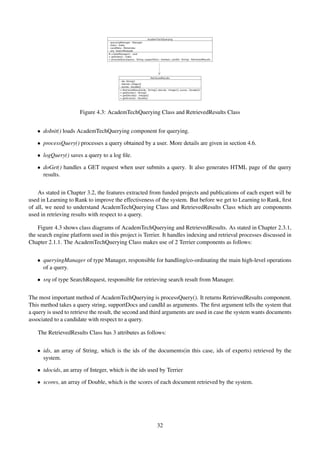
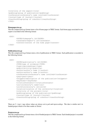
• processQuery() is a method that retrieve documents (experts) with respect to publication query and project
query.
• setScores() is a method that performs a union between results with respect to publication query and project
query as discussed in Section 3.2.2
• setFeatures() is a method that extracts features for each document (expert) and write into a LETOR file.
• learnModel() is a method that produces a learned model using RankLib.
As stated in Chapter 2.3.2, learning to rank algorithms used in this project are AdaRank and Coordinate
Ascent. The performance of each of them will be discussed in Evaluation Section. Figures 4.7 and 4.8 show
learned models using Coordinate Ascent and AdaRank Algorithms. Section 4.6 will explain a component used
to apply a learned model.
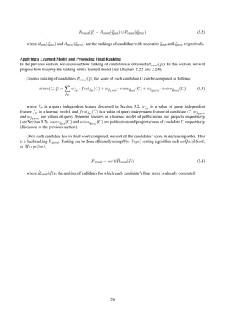
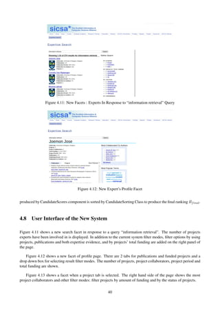
4.6 Applying a Learned Model and Producing Final Ranking
In Chapter 3.2.2, we explained the process of applying a learned model and generating a final ranking. This
section aims to describe components that handle these tasks. The class CandidateScores has a method called,
getTotalScore() taking a learnedModel component as a parameter. This method applies a learned model as
described in Chapter 2.2.6 and returns a score associated with an expert. Figure 4.9 shows class diagrams of
Candidatescores and LearnedModel.
The CandidateScores is used for computing scores of candidates based on a learned model. The Candi-
dateSorting sorts scores of candidates obtained after applying a learned model in descending score. The sorting
algorithm applied in this class is merge sort [5], giving time complexity of O(n · log n) where n is the number
38](https://image.slidesharecdn.com/4fde60ad-44a6-4bcf-8ac2-2d1594a4aa54-160724173420/85/dissertation-41-320.jpg)


![Chapter 5
Evaluation
This chapter is aimed to demonstrate that applying LETOR technique improves the effectiveness of the expert
search system. It separates into 2 experiments. The first experiment does not make use of K-fold Cross-validation
technique (see Section 5.1) but the second experiment does (see Section 5.2). We use LETOR technique proposed
in Chapter 2.2. Basically, there are 2 necessary datasets: training and testing datasets and 1 optional dataset:
validation dataset. In IR, we refer them as training, testing and validation queries respectively. Some of the
queries were provided by Dr. Craig Macdonald and the others were made up by myself. We made an assumption
that the current system (using only publication as expertise evidence) is effective. This means that relevance
judgements (the experts retrieved in response to a query) can be obtained manually from the current system.
To make relevance judgements, top 20 experts retrieved in response to a query are examined if they are truly
an expert by visiting their official home page and with the help of Dr. Craig Macdonald. Since constructing
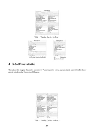
relevance judgements is time-consuming, we have made only 67 queries. Throughout this chapter, the queries
annotated by * denote queries whose relevant experts are restricted to those experts only from the University of
Glasgow. It is difficult to judge experts not in the University of Glasgow because we do not know them. However,
in practice, this will incur dataset quality [19].
Before we discuss evaluation, we should have some goals set up. This is necessary because the evaluation
results can be compared against the goals in order to conclude whether all goals are achieved or not. As stated
in Chapter 1.3, our goal is to integrate new kind of expertise evidence, funded projects, with existing expertise
evidence, publications, to enhance the effectiveness of the expert search system. At the end of this chapter, we
have to be able to answer the following question:
Does integrating funded projects with publications using learning to rank technique (LETOR)
help improve the effectiveness of the expert search system?
We refer to a currently deployed SICSA expert search system (without Learning to Rank) as our baseline.
This term will be frequently used throughout this chapter.
5.1 Evaluation Without K-fold Cross-validation
This section is aimed to demonstrate that applying LETOR technique improves the effectiveness of the deployed
expert search system. K-fold Cross-validation technique is not applied in this section.
43](https://image.slidesharecdn.com/4fde60ad-44a6-4bcf-8ac2-2d1594a4aa54-160724173420/85/dissertation-46-320.jpg)

![Testing Queries Expert Grade Rank (Coordinate Ascent) Rank (Baseline)
*force feedback Stephen Brewster 2 1 1
Roderick Murray-Smith 2 N/A N/A
*human error health care Stephen Robert 1 3 3
*information extraction Joemon Jose 2 8 8
Alessandro Vinciarelli 1 4 4
*haptic visualisation Stephen Brewster 2 1 1
Roderick Murray-Smith 2 N/A 5
John Williamson 2 4 9
Phillip Gray 2 N/A 6
information retrieval Joemon Jose (Glasgow University) 2 1 1
Cornelis Van Rijsbergen (Glasgow University) 2 2 2
Craig Macdonald (Glasgow University) 1 4 4
Iadh Ounis (Glasgow University) 2 5 5
Leif Azzopardi (Glasgow University) 1 6 6
Victor Lavrenko (Edinbugh University) 1 8 8
robotics Sethu Vijayakumar (Edinbugh University) 2 1 1
Subramanian Ramamoorthy (Edinbugh University) 1 7 7
Andrew Brooks (Dundee University) 1 4 4
Clare Dixon (Glasgow University) 1 9 9
Katia Sycara (Aberdeen University) 2 10 10
Table 5.5: Ranking Evaluation
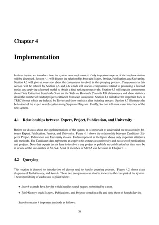
Table 5.4 shows the evaluation results of each testing query. Numbers in bold are numbers higher than ones
in the baseline. It has shown that applying LETOR technique using Coordinate Ascent algorithm to the testing
queries shown in table 5.5 outperformed baseline ones considering MAP/MRR values. Experts in bold indicates
that using Coordinate Ascent they are ranked higher higher than baseline. N/A indicates that the experts are not
in the top 10 of the ranking. Experts with 0 graded relevance value are not shown in this table. Graded relevance
values of experts can be found in Appendix Chapter.
According to table 5.5, only 1 expert John Williamson retrieved with respect to testing query, haptic visuali-
sation, is ranked better than baseline.
• force feedback
• haptic visualisation
• human error heath care
• information extraction
• information retrieval
• robotics
5.2 Evaluation With K-fold Cross-validation
In the previous section, the evaluation results have shown that applying LETOR makes the deployed expert search
system perform poorer. This section aims to evaluate the effectivenes of the system by applying K-fold Cross-
validation technique described in Chapter 2.2.8. We decided to choose K = 5. This is fairly normal for learning
to rank [19]. Higher K is possible, but that infers that the LETOR needs more training. RankLib provides K-fold
Cross-validation functionality. However, we will not use this functionality because some of our datasets results
were restricted to those experts only from the University of Glasgow. For this reason, the datasets should be split
into training, validation and testing queries manually to avoid one of them having only experts from University
of Glasgow [19].
5.2.1 Experimental Setting
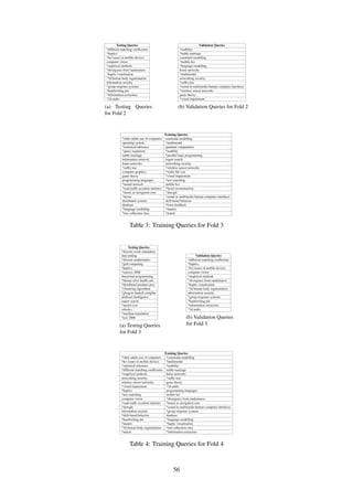
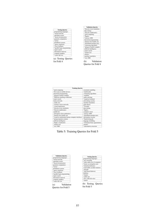
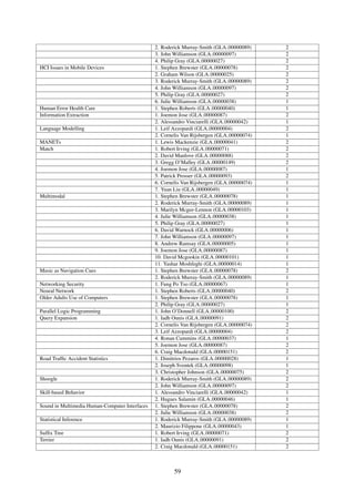
As discussed earlier, we decided to choose K = 5 for K-fold Cross-validation. Each of the 5 folds has all of the
queries: 60% for training, 20% for validation and 20% for testing [3]. Across the 5 folds, each query will appear
46](https://image.slidesharecdn.com/4fde60ad-44a6-4bcf-8ac2-2d1594a4aa54-160724173420/85/dissertation-49-320.jpg)
![Testing Queries Expert Grade Rank (Coordinate Ascent) Rank (Baseline)
artificial intelligence David Bell (Strathclyde University) 1 1 1
Ruth Aylett (Heriot Watt University) 2 2 2
Alan Smaill (Edinburgh University) 1 7 7
Alan Bundy (Edinburgh University) 1 9 9
*ecir 2008 Iadh Ounis 2 2 2
Craig Macdonald 2 1 1
Joemon Jose 2 8 8
*force feedback Stephen Brewster 2 1 1
Roderick Murray-Smith 2 8 8
information retrieval Joemon Jose (Glasgow University) 2 1 1
Cornelis Van Rijsbergen (Glasgow University) 2 2 2
Craig Macdonald (Glasgow University) 1 4 4
Iadh Ounis (Glasgow University) 2 5 5
Leif Azzopardi (Glasgow University) 1 6 6
Victor Lavrenko (Edinbugh University) 1 8 8
Table 5.6: Ranking Evaluation using K-fold Cross-validation
Algorithm MAP NDCG MRR Number of Relevant Experts
AdaRank 0.0469 0.2397 0.0843 106
Coordinate Ascent 0.5321 0.6703 0.6366 106
Without LETOR 0.5499 0.6871 0.6484 106
Table 5.7: Evaluation Results Using K-fold Cross-validation
3 times in training, once in validation and once in testing queries. For each fold, training queries are trained and
validated by validation queries to obtain a learned model. Then a learned model for each fold is applied to testing
queries of that fold. Results of each run across the 5 folds are combined into one results file in TREC format.
With the qrels file, this results file is then evaluated with trec eval. Finally, one of the learned models is used by
the system. Testing, training and validation queries for each fold can be found on Appendix.
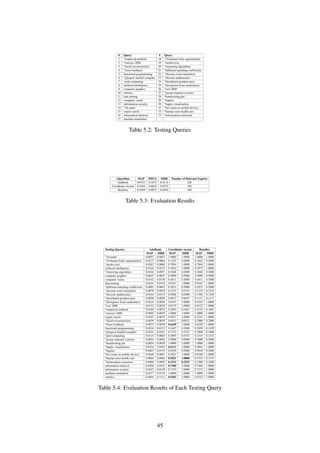
5.2.2 Experimental Results
Table 5.7 shows the retrieval effectiveness of the proposed LETOR techniques using K-fold cross-validation
techinque and retrieval effectiveness of the baseline. It can be clearly seen that overall the baseline is still
better than LETOR using K-fold cross-validation. Coordinate Ascent still gives second best performance. But
using K-fold cross-validation technique, the effectiveness is slightly better than not using K-fold cross-validation
(discussed in the last section). Therefore, the answer to the question is still NO, using LETOR technique with
K-fold cross-validation does not enhance the effectiveness of the deployed expert search system. Table 5.8 shows
the evaluation results of each testing query. Numbers in bold show testing queries applying Coordinate Ascent
whose evaluation metrics are higher than baseline ones. Numbers underlined show that testing queries applying
AdaRank algorithm perform better than ones applying Coordinate Ascent. The evaluation results of the testing
queries applied with LETOR using Coordinate Ascent shown in table 5.6 outperform baseline ones considering
MAP/MRR values. Experts shown in table 5.6 in the top 10 of the ranking are analysed to if the ranking with
LTR using K-fold Cross-validation is better than baseline. Experts with 0 graded relevance value are not shown
in this table. Graded relevance values of experts can be found in Appendix Chapter. According to table 5.5,
applying K-fold Cross-validation change the ranking compared to the baseline.
5.3 Causes of Learning to Rank Failure
It has shown in the last section that applying LETOR technique fails. The followings are reasons behind it [19]:
• The size of training/validation dataset is not big enough.
• Selected LETOR Features are not very useful.
47](https://image.slidesharecdn.com/4fde60ad-44a6-4bcf-8ac2-2d1594a4aa54-160724173420/85/dissertation-50-320.jpg)
![Testing Queries AdaRank Coordinate Ascent Without LETOR
MAP MRR MAP MRR MAP MRR
3d audio 0.0227 0.0227 1.0000 1.0000 1.0000 1.0000
3d human body segmentation 0.0239 0.0222 0.1824 0.2000 0.1824 0.2000
anchor text 0.0263 0.0088 0.7894 1.0000 0.7894 1.0000
artificial intelligence 0.0344 0.0233 0.6064 1.0000 0.5972 1.0000
clustering algorithms 0.0166 0.0071 0.3048 0.2000 0.3048 0.2000
computer graphics 0.1429 0.1429 0.5000 0.5000 0.5000 0.5000
computer vision 0.0430 0.0667 0.4611 0.5000 0.4611 0.5000
data mining 0.0181 0.0118 0.9167 1.0000 0.9167 1.0000
different matching coefficients 0.0076 0.0052 0.5833 0.5000 0.5833 0.5000
discrete event simulation 0.0078 0.0078 0.3333 0.3333 0.3333 0.3333
discrete mathematics 0.0164 0.0115 0.1214 0.1000 0.1394 0.1250
distributed predator prey 0.0058 0.0058 0.0038 0.0038 0.1111 0.1111
divergence from randomness 0.0205 0.0122 0.9167 1.0000 0.9167 1.0000
ecir 2008 0.0152 0.0070 0.8304 1.0000 0.8125 1.0000
empirical methods 0.0316 0.0286 0.2154 0.1667 0.2154 0.1667
eurosys 2008 0.0055 0.0055 1.0000 1.0000 1.0000 1.0000
expert search 0.0106 0.0076 0.5040 1.0000 0.5227 1.0000
facial reconstruction 0.0270 0.0270 0.1429 0.1429 0.2000 0.2000
force feedback 0.5141 1.0000 0.6429 1.0000 0.6250 1.0000
functional programming 0.0244 0.0112 0.0952 0.1111 0.2038 0.1429
glasgow haskell compiler 0.0101 0.0101 0.3333 0.3333 0.5000 0.5000
grid computing 0.0123 0.0083 0.3333 0.3333 0.3333 0.3333
group response systems 0.0047 0.0047 0.5000 0.5000 0.5000 0.5000
handwriting pin 0.0422 0.0400 1.0000 1.0000 1.0000 1.0000
haptic visualisation 0.0328 0.0400 0.5861 1.0000 0.5861 1.0000
haptics 0.0331 0.0104 0.4091 0.5000 0.5819 0.5000
hci issues in mobile devices 0.0319 0.0357 0.6160 1.0000 0.6160 1.0000
human error health care 0.0064 0.0064 0.3333 0.3333 0.3333 0.3333
information extraction 0.0254 0.0217 0.2500 0.2500 0.2500 0.2500
information retrieval 0.2538 1.0000 0.7622 1.0000 0.7468 0.7468
information security 0.0275 0.0476 0.7333 1.0000 0.7333 1.0000
machine translation 0.0117 0.0118 1.0000 1.0000 1.0000 1.0000
robotics 0.0404 0.1111 0.5523 1.0000 0.5523 1.0000
Table 5.8: Evaluation Results of Each Testing Query Using K-fold Cross-validation
• The number of publications and funded projects is not balanced. We have 22225 publications but only
369 funded projects. This results in features related to publications outweighing funded project features in
both query dependent and independent features.
For AdaRank, the performance is considerably poorer than Coordinate Ascent because AdaRank requires a large
set of validation data to avoid overfitting [19]. Therefore, we decided to apply K-fold Cross-validation technique
as it gave better performance compared to not applying K-fold Cross-validation technique (see last section).
48](https://image.slidesharecdn.com/4fde60ad-44a6-4bcf-8ac2-2d1594a4aa54-160724173420/85/dissertation-51-320.jpg)
![Chapter 6
Conclusions
In this project, we applied 2 LETOR algorithms: AdaRank and Coordinate Ascent, to combine different kinds of
expertise evidence in order to improve the performance of the system. There are various LETOR algorithms used
in industry such as LambdaMART, Random Forests etc. However, AdaRank and Coordinate Ascent algorithms
are chosen due to its simplicity and effective performance. Our experimental results (see last chapter) have shown
that
• AdaRank does not perform very well compared to Coordinate Ascent.
• Applying LETOR does not improve the performance of the system.
The reasons behind LETOR failure can be found in the previous chapter.
6.1 Requirements Achieved
The following is a summary of the requirements (see Chapter 3.2.1) that have been achieved.
• All of the system’s Must Have requirements.
• All of the system’s Should Have requirements.
• All of the non-functional Requirements.
The system’s Would like to Have and Could Have requirements could not be achieved because of time constraint.
The Could Have requirements can be difficult for 4th year students [19] as they are too complex and require full
understanding of the behaviours of the technique used [19]. However, the aim of the project is to experiment 2
LETOR algorithms: AdaRank and Coordinate, and apply the one performing better.
6.2 Challenges
During the development of the project, we have encountered various challenges. This section will discuss chal-
lenges encountered.
49](https://image.slidesharecdn.com/4fde60ad-44a6-4bcf-8ac2-2d1594a4aa54-160724173420/85/dissertation-52-320.jpg)
![6.2.1 LETOR
Learning to rank is a relatively new field in which machine learning algorithms are used to learn this ranking
function [37]. It is of particular importance for search engines to accurately tune their ranking functions as it
directly affects the search experience of users [37]. Choosing the right LETOR technique is research based and
it requires an understanding of the LETOR techniques behaviours which could possibly take weeks or months to
come up with the best approach.
6.2.2 Relevance Judgement
Relevance judgement (see chapter 5) by human assessors is considered one of the most difficult parts in this
project since it is based on person’s experience [32]. For this reason, constructing good quality training, testing
and validating datasets is also a challenge as it directly affects the performance of the system [19].
6.3 Problems Encountered
During the development of the project, we have encountered various problems. Some of them can be addressed
and some can not. In this section, we list a number of problems encountered during development life cycle.
6.3.1 Expert’s Name Pattern Matching
In Chapter 4.3, we discussed approaches used to handle differences between expert’s name formats in each
funded projects datasource. Still, we have problems regarding pattern matching between expert’s names from
Grant on the Web [1]. Consider Professor Joemon Jose, he is currently a professor in computing science at
Glasgow University. Grant on the Web records his name as Jose, Professor JM. This makes it impossible to
accurately pattern match the name with our known candidates if there are experts named Professor Joemon Jose
and Professor Jasmine Jose because Grant on the Web will record their names in the same format: Jose, Professor
JM. Although we could solve the problem by taking the university they are lecturing into account, the problem
still exists if they are from the same university.
6.3.2 Lack of LETOR Algorithms Explanation
Clear explanations of the Coordinate Ascent and AdaRank LETOR algorithms are difficult to find. Trying to
understand the nature of the algorithms is not an easy task for 4th year student as it is based on mathematics and
statistics.
6.3.3 Poor Quality of Relevance Judgements
In Chapter 5, we talked about the problems we encountered when constructing relevance judgements. That is,
we managed to construct training queries whose results (relevant experts) are only from University of Glasgow
(see last chapter). The reason behind this is that it is difficult to judge experts not in University of Glasgow
because we do not know them. As a consequence of poor relevance judgements, the dataset used for training and
evaluation becomes poor [19].
50](https://image.slidesharecdn.com/4fde60ad-44a6-4bcf-8ac2-2d1594a4aa54-160724173420/85/dissertation-53-320.jpg)
![6.4 How would I have done differently?
In Sections 6.2 and 6.3, we discussed challenges and problems encountered during the development of the system.
However, these issues could be minimised or eliminated if
• The behaviours of LETOR algorithms is well understood at the early stage of the development - this means
that we could experiment only suitable algorithms whose behaviour is applicable to the task.
• Various funded projects datasources should be used to increase the number of expertise evidence - this
means that we would have more training, validation and testing datasets.
• Relevance Judgements are prepared by experienced persons - this means that the performance of LETOR
techniques could be enhanced as relevance judgements are used to produce training and validation datasets.
6.5 Future Work
In the previous chapter, the experimental results have shown that applying LETOR techniques using AdaRank
and Coordinate Ascent algorithms does not improve the performance of the system. This might not be true
however, if the system applies other LETOR algorithms provided by RankLib since each algorithm has its own
behaviours. In addition, good training/validation datasets and feature selections play the main roles to the per-
formance of the system [19]. I strongly believe that the intuitions (features) proposed in Chapter 3.2 are very
useful but the main reason why LETOR fails is due to small training dataset. We had 34 training queries which is
very small. Each testing query can be analysed to determine why applying a learned model gives better or worse
performance compared to not applying LETOR. This can be done by for example, analysing the number of all
terms, the number of funded projects terms and of publications terms relevant to each testing query.
Moreover, for IR systems to get better performance, not only LETOR technique is contributed to the success
of the retrieval system, but also other aspects in IR such as tokenisation technique, stemming technique and
retrieval models. LETOR is just an optional technique in machine learning used to optimise the ranking based
on training/validation datasets. However, all of these aspects should be experimented.
51](https://image.slidesharecdn.com/4fde60ad-44a6-4bcf-8ac2-2d1594a4aa54-160724173420/85/dissertation-54-320.jpg)
![Bibliography
[1] Engineering and physical sciences research council (epsrc). http://gow.epsrc.ac.uk/.
[2] Information retrieval. http://en.wikipedia.org/wiki/Information_retrieval.
[3] K-fold cross-validation. http://en.wikipedia.org/wiki/Cross-validation_
(statistics)#K-fold_cross-validation.
[4] Learning to rank. http://en.wikipedia.org/wiki/Learning_to_rank.
[5] Merge sort. http://en.wikipedia.org/wiki/Merge_sort.
[6] Pagerank. http://en.wikipedia.org/wiki/PageRank.
[7] Polymorphism. http://en.wikipedia.org/wiki/Polymorphism_(computer_science).
[8] qrels file. http://www.mpi-inf.mpg.de/˜dfischer/manual/manual_qrelformat.
html.
[9] Ranklib. http://sourceforge.net/p/lemur/wiki/RankLib/.
[10] Relevance judgement file list. http://trec.nist.gov/data/qrels_eng/.
[11] Research councils uk - gateway to research. http://gtr.rcuk.ac.uk/.
[12] The scottish informatics and computer science alliance expert search system. http://experts.
sicsa.ac.uk/.
[13] The scottish informatics and computer science alliance (sicsa). http://www.sicsa.ac.uk/home/.
[14] Terrier. http://www.terrier.org/.
[15] The text retrieval conference (trec). http://trec.nist.gov/overview.html.
[16] Trec result file format. http://ir.iit.edu/˜dagr/cs529/files/project_files/trec_
eval_desc.htm.
[17] Information retrieval system evaluation. http://nlp.stanford.edu/IR-book/html/
htmledition/information-retrieval-system-evaluation-1.html, 2009.
[18] Inverted index. http://en.wikipedia.org/wiki/Inverted_index, 2012.
[19] Conversation of dr. craig macdonald, 2014.
[20] Discounted cumulative gain. http://en.wikipedia.org/wiki/Discounted_cumulative_
gain, 2014.
[21] Mean reciprocal rank. http://en.wikipedia.org/wiki/Mean_reciprocal_rank, 2014.
52](https://image.slidesharecdn.com/4fde60ad-44a6-4bcf-8ac2-2d1594a4aa54-160724173420/85/dissertation-55-320.jpg)
![[22] Search engine. http://en.wikipedia.org/wiki/Search_engine_(computing), 2014.
[23] Term frequency–inverse document frequency (tf-idf). http://en.wikipedia.org/wiki/Tf%E2%
80%93idf, 2014.
[24] Tokenization. http://en.wikipedia.org/wiki/Tokenization, 2014.
[25] Web search engine. http://en.wikipedia.org/wiki/Web_search_engine, 2014.
[26] Iadh Ounis Craig Macdonald. Voting for candidates: Adapting data fusion techniques for an expert search
task. pages 387, 388, 389, 2006.
[27] Rodrygo L.T. Craig Macdonald and Iadh Ounis. About learning models with multiple query dependent
features. 2012.
[28] Prof. Joemon M Jose. Architecture of retrieval systems, 2013.
[29] Prof. Joemon M Jose. Information retrieval, 2013.
[30] Prof. Joemon M Jose. Information retrieval - evaluation methodology, 2013.
[31] Prof. Joemon M Jose. Probabilistic retrieval model, 2013.
[32] Professor Joemon Jose. Text classification, 2013.
[33] Hang Li. Learning to Rank for Information Retrieval and Natural Language Processing. 2011.
[34] Craig Macdonald. The Voting Model for People Search. PhD thesis, Department of Computing Science,
Faculty of Information and Mathematical Sciences, University of Glasgow, 2009.
[35] Afshin Rostamizadeh Mehryar Mohri and Ameet Talwalkar. Foundations of Machine Learning. The MIT
Press, 2012.
[36] Donald Metzler. Automatic feature selection in the markov random field model for information retrieval.
[37] Yi Chang Olivier Chapelle. Yahoo! learning to rank challenge overview. 2011.
[38] Mark Girolami Simon Rogers. A First Course in Machine Learning. 2011.
53](https://image.slidesharecdn.com/4fde60ad-44a6-4bcf-8ac2-2d1594a4aa54-160724173420/85/dissertation-56-320.jpg)