This thesis presents a framework for integrating hard sensor data and soft data sources, like incident reports, to improve maritime situational awareness and automated course of action generation. The framework extends an existing Risk Management Framework to incorporate soft data features into risk modeling and evaluation. It also includes soft data, like subject matter expertise, to generate more effective response plans. The framework is validated using real and synthetic maritime scenarios. Performance is evaluated using metrics like information fusion effectiveness and ability to handle uncertainties. The results demonstrate the framework can provide more accurate and timely situational updates by integrating different data sources.

![viii
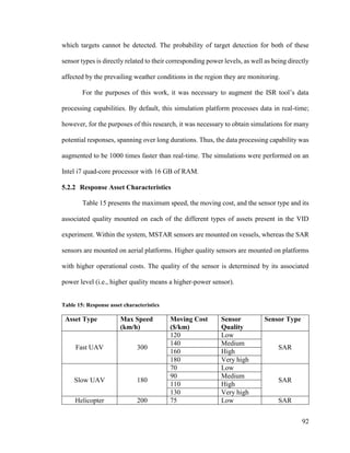
List of Figures
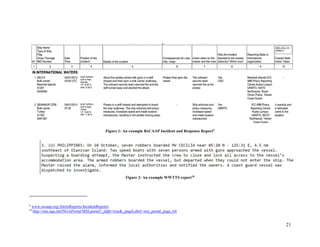
Figure 1: An example ReCAAP Incident and Response Report ............................................ 21
Figure 2: An example WWTTS report ................................................................................... 21
Figure 3: Track crawl search pattern, as presented in [66]..................................................... 22
Figure 4: Parallel track line search pattern, as presented in [65]............................................ 23
Figure 5: Outwards expanding square search pattern, as presented in [65]............................ 23
Figure 6: The RMF's SA components, adapted from [12]...................................................... 27
Figure 7: DTG Module ........................................................................................................... 28
Figure 8: Instantaneous information fusion effectiveness (i-IFE) hierarchy .......................... 37
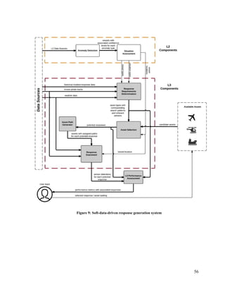
Figure 9: Soft-data-driven response generation system.......................................................... 56
Figure 10: Example synthetic incident report with L3 information ....................................... 60
Figure 11: Example response grid with three designated subgrids......................................... 62
Figure 12: Adhoc search pattern generation algorithm........................................................... 64
Figure 13: Custom Mutation Operator.................................................................................... 67
Figure 14: Maritime incident distribution per incident category............................................ 75
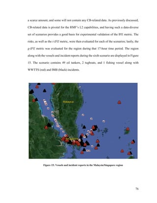
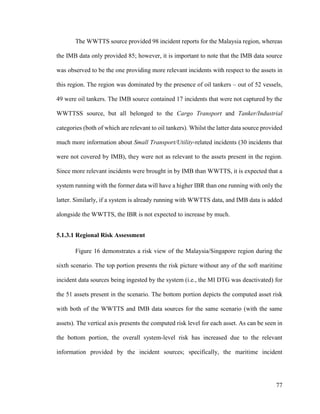
Figure 15: Vessels and incident reports in the Malaysia/Singapore region............................ 76
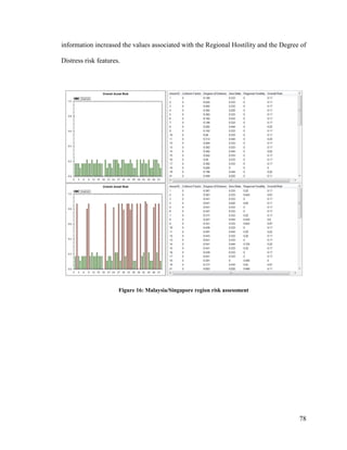
Figure 16: Malaysia/Singapore region risk assessment.......................................................... 78
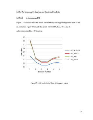
Figure 17: i-IFE results in the Malaysia/Singapore region..................................................... 79
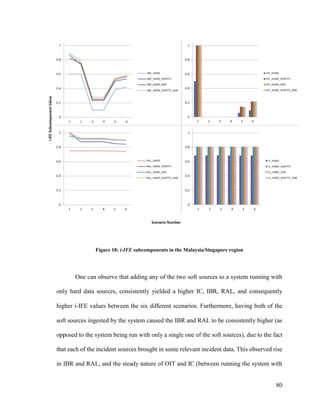
Figure 18: i-IFE subcomponents in the Malaysia/Singapore region ...................................... 80
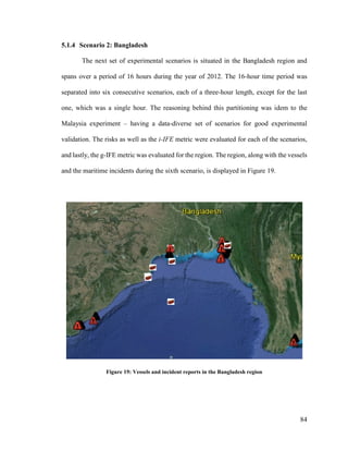
Figure 19: Vessels and incident reports in the Bangladesh region ......................................... 84
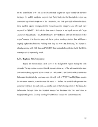
Figure 20: Bangladesh region risk assessment ....................................................................... 86
Figure 21: i-IFE results in the Bangladesh region.................................................................. 87](https://image.slidesharecdn.com/14ada79c-c8c9-462e-aceb-00c958cdaf17-161228170344/85/Plachkov_Alex_2016_thesis-8-320.jpg)
![1
Chapter 1. Introduction
Maritime Domain Awareness (MDA) can be summarized as the situational
knowledge of physical and environmental conditions that exist within or influence a
maritime region. The intended scope of this awareness includes all behaviours that could,
directly or indirectly, affect the security of the region, its economic activity or the local
environment [1] [2]. MDA is achieved via persistent monitoring of the maritime
environment, which allows for the identification of common trends and thus the detection
of anomalous behaviour. Achieving effective MDA also entails the efficient tasking of
maritime assets to counter illegal activities, as well as to assist in search and rescue (SAR)
efforts.
In order to obtain accurate MDA, information derived from multiple data sources
must be effectively captured, seamlessly integrated, and efficiently reasoned upon. Initial
solutions attempted to resolve these challenges through the use of low-level Information
Fusion (IF) modules; however, as the available data experienced exponential growth (in
terms of variety, volume, velocity, and veracity), these low-level modules became
inadequate [1]. To overcome this challenge, also referred to as the Big Data Problem, much
research has gone into the development and use of High-Level IF (HLIF) techniques. HLIF
is defined as Level 2 (L2) Fusion and above in the Joint Director of Laboratories
(JDL)/Data Fusion Information Group (DFIG) models [3] [4], and has been successfully
tasked with carrying out MDA processes (e.g., anomaly detection, trajectory prediction,
intent assessment, and threat assessment) [1] [5].
Traditionally, IF systems have relied on the use of ‘hard’ data, that is, data provided
by physical sensors, such as acoustic, radar, global positioning system (GPS), sonar, or](https://image.slidesharecdn.com/14ada79c-c8c9-462e-aceb-00c958cdaf17-161228170344/85/Plachkov_Alex_2016_thesis-15-320.jpg)
![2
electro-optical sensors. This data is objective, structured, and quantitative, and maritime
operators often rely on hard data generated by vessel traffic in order to identify anomalous
or suspicious events at sea. Recently however, the IF community has recognized the
potential of exploiting information generated by ‘soft’ sensors (that is, people-generated
information). Conversely, this type of data is more subjective, qualitative, and transcribed
in a semi-structured or unstructured format (e.g., free form natural language text). Soft data
can be rich in context and provide cognitive inferences not otherwise captured by
traditional sensors (e.g., judged relationships among entities and/or events) and can thus be
used to further augment the situational awareness picture of the system. The exploitation
of this type of data, however, comes at a cost, as its content can be exposed to
bias/subjectivity, inaccuracy, imprecision, low repeatability, and conflict [6] [7]. Examples
of soft data sources in the maritime domain include textual reports on vessel sightings or
detailed descriptions of maritime incidents. It is therefore not surprising to see recent
attempts to construct and evaluate Hard-Soft IF (HSIF) frameworks [8] [9], as well as
efforts to incorporate soft information in maritime decision making like in [10], where
Natural Language Processing (NLP) methods were employed to draw out meaningful
information from soft data sources.
An HLIF system capable of constructing a risk-aware view of the environment (and
the dynamic entities within) can enable the proactive identification of hazards, dangers,
and vulnerabilities, which subsequently leads to the generation of suitable countermeasures
to mitigate said risks. Such a system has already been proposed in [11] [12] and termed by
the authors the Risk Management Framework (RMF), but considers only hard data sources.](https://image.slidesharecdn.com/14ada79c-c8c9-462e-aceb-00c958cdaf17-161228170344/85/Plachkov_Alex_2016_thesis-16-320.jpg)
![3
1.1 Motivation
Maritime piracy and armed robbery at sea is estimated to cost the worldwide
economy annually anywhere between $1 Billion to $16 Billion US dollars1
, whilst SAR
efforts are estimated to cost the US coast guard alone approximately $680 Million USD
yearly2
. These numbers present a strong need for automated solutions in securing the
maritime areas by providing accurate and timely situational updates and assisting in
operational decision making. There are recent organizational initiatives to support
increased collaboration and maritime information sharing among participating nations
through internet networks precisely for this purpose, such as: (1) the Information Fusion
Centre (IFC) hosted by the Singapore Navy, where 35 countries are exchanging data and
collaborating on maritime operations, such as piracy hijacking events and SAR missions3
;
(2) the Information Sharing Centre (ISC) of the Regional Cooperation Agreement on
Combating Piracy and Armed Robbery against Ships in Asia (ReCAAP), also based in
Singapore, with a total of 20 currently collaborating nations4
; and (3) the International
Maritime Bureau’s Piracy Reporting Centre (IMB PRC), located in Malaysia, which is
responsible for disseminating piracy incident data to maritime security agencies around the
world [13].
1.2 Contributions
This study focuses on extending the RMF’s L2 and L3 fusion capabilities through
the inclusion of soft data for the purpose of increased SA and improved CoA generation.
1
http://worldmaritimenews.com/archives/134829/annual-global-cost-of-piracy-measured-in-billions/
2
http://www.theday.com/article/20091219/INTERACT010102/912199999/0/SHANE
3
https://www.mindef.gov.sg/imindef/press_room/official_releases/nr/2014/apr/04apr14_nr/04apr14_fs.html
4
http://www.recaap.org/AboutReCAAPISC.aspx](https://image.slidesharecdn.com/14ada79c-c8c9-462e-aceb-00c958cdaf17-161228170344/85/Plachkov_Alex_2016_thesis-17-320.jpg)
![6
Chapter 2. Background and Related Work
2.1 Maritime Risk Analysis
Risk can be formally defined as the effect of uncertainty on an entity's objectives
[14]. A fundamental objective in MDA is the achievement of a comprehensive level of
situational awareness (SAW), and within this domain, uncertainty corresponds to the lack
of information to support such a level. SAW is defined as a state of knowledge of the
environment, achieved and maintained through one or many SA processes [15].
Augmenting the degree of SAW in MDA can be broken down into a number of sub-
problems, such as the enhancement of the collection and dissemination of data, as well as
the improvement of the multitude of algorithms involved in its processing. Popular
techniques employed for evaluating risk are probabilistic models, such as Bayesian
Networks in [16] [17], Hidden Markov Models (HMMs) in [18] [19], and Evidence-based
models in [20]. The common drawback of these approaches is that they greatly rely on a
priori knowledge, derived from statistical analysis of large collections of historical data
(e.g., event occurrence probabilities). Computational Intelligence (CI) techniques have also
been employed, such as in [12] and [21] where some of the risk features of assets are
quantified via Fuzzy Systems (FS). FS provide a natural, interpretable, yet effective basis
for incorporating domain expert knowledge into the risk assessment process.](https://image.slidesharecdn.com/14ada79c-c8c9-462e-aceb-00c958cdaf17-161228170344/85/Plachkov_Alex_2016_thesis-20-320.jpg)
![7
2.2 High-Level Information Fusion for Maritime Domain Awareness
Machine learning algorithms that are employed in the maritime domain aim to
detect anomalies, or abnormal behaviors, in vessel activity data. Typically, these
algorithms are trained using information pertaining to normal vessel activities in order to
learn a normalcy model, and, when operational, they are used to detect any behaviour
deviating from that model (i.e., anomalous behaviour). Recent HLIF techniques that have
been employed for anomaly detection include neural networks [22] [23] [24], probabilistic
models [25] [26] [27] [28] [29] [30], clustering approaches [24] [31] [32] [33], as well as
evolutionary algorithms [34] [35]. These techniques typically fall under two categories –
unsupervised vs. supervised. Unsupervised techniques are popular due to their self-
governing nature – namely, their ability to discover hidden, meaningful structure in
unlabeled data. A good argument can, however, be made for supervised techniques, since
they incorporate domain expert knowledge into the learning process in the form of labelled
training data.
The benefit of including human operators and analysts in the anomaly detection
process itself (i.e., when the system is online) has been greatly underestimated in the
maritime domain [36]. For this reason, the involvement of people in traditional systems
has largely been only up to the point of constructing the anomaly model. There have been
recent attempts to incorporate humans into the MDA processes, such as in [22], where the
system can be directed for continuous online learning via operator intervention. Such
evolving systems are well-suited for large, complex, dynamic environments like the
maritime domain. Some recent research efforts [36] [37] are geared towards identifying](https://image.slidesharecdn.com/14ada79c-c8c9-462e-aceb-00c958cdaf17-161228170344/85/Plachkov_Alex_2016_thesis-21-320.jpg)
![8
potential areas for visualization and human interaction during the anomaly detection
process for improving the performance of the detectors.
Within the Joint Director of Laboratories (JDL)/Data Fusion Information Group
(DFIG) models [3] [4] [38], Level 2 (L2) and Level 3 (L3) Information Fusion (IF) are
respectively defined as SA and Impact Assessment (IA), with the term High-Level IF
(HLIF) being defined as L2 and above. The role of L2 Fusion is to characterize the
presently unfolding situations through the automated analysis and identification of
relations existing between the entities being monitored, as well as between the entities and
the environment they reside in. Upon successful characterization of situations, L3 Fusion
proceeds with generating CoA recommendations and estimating their effects on the known
situations. Both levels have been successfully tasked with carrying out typical MDA
processes (e.g., anomaly detection, trajectory prediction, intent assessment, and threat
assessment) [1] [5]. The automatic generation of suitable CoAs in the maritime domain
using evolutionary multi-objective optimization (EMOO) has been addressed before in
[12] and [21] but considering only hard data sources. Soft data has been employed in [10]
at L2 Fusion to extract risk factors from reported maritime incidents. No studies in the
maritime world appear to consider supplementing or augmenting CoA generation through
the use of soft data.
2.3 Data in High-Level Information Fusion
Two broad categories of data exist in the IF domain, namely, hard and soft. Hard
data is generated by physical sensors, and hence it is typically provided in a numeric
format. Characteristics of this type of data are calibration, accuracy, structure, objectivity,
precision, repeatability, and high frequency [6] [7]. Soft data, on the other hand, is typically](https://image.slidesharecdn.com/14ada79c-c8c9-462e-aceb-00c958cdaf17-161228170344/85/Plachkov_Alex_2016_thesis-22-320.jpg)
![9
generated and transcribed by humans in intelligence reports, surveillance reports, as well
as open source and social media [39] [40]. This type of data is provided in a textual format
which can either be structured (e.g., restricted language such as Controlled English [41])
or unstructured (e.g., free-form natural language). The exploitation of the information
provided by soft sensors comes at a cost, as its content can be exposed to bias/subjectivity,
inaccuracy, imprecision, low repeatability, and conflict [6] [7]. Soft data is incorporated
into HLIF systems by being processed through: Information Extraction (IE) modules,
Common Referencing (CR) modules, and Data Association (DA) modules.
IE modules attempt to draw out information of interest from each of the data
sources. The construction of the IE modules for soft data sources requires the elicitation of
a lexicon – a dictionary of terms that embody factors and entities of interest in the
environment [10]. This lexicon is then used for their automatic identification and
extraction.
CR modules convert the content provided by IE modules into a common format via,
for instance: (1) uncertainty alignment [42], as the heterogeneous data sources may express
it in inconsistent forms (e.g., hard sensor uncertainty is expressed in
probabilistic/quantitative format whereas soft sensor uncertainty is stated in
possibilistic/fuzzy terms due to the qualitative nature of linguistic expression); or (2)
temporal alignment [43], which is required when the disparate data sources present
temporal features in incongruent forms (e.g., exact timestamp vs. approximate time of day
vs. linguistic phrasing encompassing multiple verbal tense expressions).
The responsibility of DA modules is to effectively associate all of the available
evidence (from each of the data sources) for a unique entity. The same entities in the](https://image.slidesharecdn.com/14ada79c-c8c9-462e-aceb-00c958cdaf17-161228170344/85/Plachkov_Alex_2016_thesis-23-320.jpg)
![10
environment being monitored can be characterized by multiple data sources, and thus, the
DA module must effectively join all of the available data for an entity into a single,
cumulative data structure (also frequently referred to as ‘cumulative evidence structure’)
[44].
2.3.1 Soft Data Categories
There are four distinct categories of soft data:
a. Observational data [40] [41] consists of reports written by human observers (e.g.,
intelligence data written by soldiers reporting on their patrol activities). It is
typically communicated in natural language. This type of data is semantically rich,
and when provided in a ‘controlled language’ format, it can reduce the
impreciseness and uncertainty. It can be, however, ambiguous and biased,
especially when not presented in a ‘controlled language’. Observational data is also
uncalibrated – two humans observing the same situation may provide different,
even conflicting, information about the situation.
b. Contextual data [40] [42] [45] [46] contains information that can be used to
characterize a situation or the surrounding environment of one; it is said to
‘surround’ a situation. This is information which does not characterize the entities
of interest in an IF system, but rather the environment in which they reside or the
situations to which they appertain. Contextual information is of two types: static
(e.g., GIS database) and dynamic (e.g., weather conditions). This type of
information is used to better understand the situation (e.g., by reducing the amount
of uncertainty present in the information extracted from the observational data
through the removal of ambiguities or addition of constraints). A large amount of](https://image.slidesharecdn.com/14ada79c-c8c9-462e-aceb-00c958cdaf17-161228170344/85/Plachkov_Alex_2016_thesis-24-320.jpg)
![11
contextual information improves the situational understanding, but because it has
to be merged with observational data, the data assimilation operations become time
costly. Contextual data is also prone to inconsistencies and errors. No generic
context representation and exploitation frameworks exist; all attempts to exploit
context are tailored for the application at hand and thus the solutions are of limited
scalability and poor adaptability. This issue is recognized by the authors of [46],
who unveil a proposal for a middleware architecture to integrate this rich
information source into IF processes.
c. Open source and social media [40] (e.g., Blogs, Twitter, Facebook) data can be very
timely and typically arrives in a large volume. Arriving in a high volume, however,
implies potential difficulties in its processing. This soft data type is also largely
unstructured and uncontrolled.
d. Ontological data [40] [47] [48] aids in better understanding the observed situations
of the world by capturing entities, processes, events, and the relationships among
them in a particular domain. Its responsibility is to capture domain knowledge;
when used in conjunction with the hard data, it can provide a more accurate
situational understanding. Like with contextual data, augmenting the observational
data with ontological information comes at a computational cost.
2.3.2 Data Imperfections
Data imperfections have been well studied in the data fusion community and can
be classified in three broad categories [49] – uncertainty, granularity and imprecision.
Uncertainty results from ignorance about the true state of the real world, and uncertain](https://image.slidesharecdn.com/14ada79c-c8c9-462e-aceb-00c958cdaf17-161228170344/85/Plachkov_Alex_2016_thesis-25-320.jpg)
![12
data often entails having an associated confidence degree between zero and one [49] [50].
Granularity refers to the ability to differentiate between different entities present in the
data. Imprecision can be further broken down into the following three categories:
vagueness, described as lacking detail in such a way that the entities in the data have no
direct correspondence with their referents in the world; ambiguity, which occurs when the
entities in the data can have more than one referent in the real world; and incompleteness,
which arises when the data possesses only partial information about the world [49] [51].
The following mathematical theories have been recently used in the HSIF
community to attempt to deal with imperfect data: Dempster-Shafer Evidence Theory
(DSET), Possibility Theory (PT), Random Finite Set Theory (RFST), and Markov Logic
Networks (MLNs). Specific details on each of the former three theories, as well as their
applicability, limitations, and use in data fusion can be found in [49]; details on MLNs can
be located in [26].
DSET was used to allow for decision making under uncertainty in a hard-soft data
fusion security system in [52], which is capable of assessing the threat level of situations
in which objects approach and/or cross a security perimeter. It was also used in [53] to
combine the uncertainties of data items in a fusion system containing only soft data.
Transferable Belief Model, an extension of DSET, was used to perform reasoning under
uncertainty and evaluation of the threat level caused by suspicious vessels in a hard-soft
data fusion system in [45]. It was also used to combine inconsistent data and assess how
much of the received data observations supported given hypotheses in a soft-data-only
fusion system in [54].](https://image.slidesharecdn.com/14ada79c-c8c9-462e-aceb-00c958cdaf17-161228170344/85/Plachkov_Alex_2016_thesis-26-320.jpg)
![13
PT was used to integrate imprecise qualitative data in a soft fusion framework in
[42], and to model the uncertainty in soft data in an SA system in [55].
RFST was used in an HSIF framework in [56] to combine data from both hard and
soft sources and enhance the performance of Kalman Evidential Filter-based target
tracking.
MLNs were used in [26] to encode domain knowledge through first order logic
(FOL) expressions; the latter were assigned associated uncertainty weights, and fused with
real-time sensor data in order to detect maritime traffic anomalies.
2.4 Performance Evaluation in Hard-Soft Information Fusion
A natural interest in the field of HSIF is the quantification of the performance of
the fusion systems. Possessing the ability to evaluate the performance of such systems is
crucial for making key design and/or runtime decisions, such as which fusion algorithms
are most suitable given the available data sources, or what subset of the data sources
provides the highest benefit to the system (for situations in which it may be
computationally intractable to process all of the available data). When it comes to
evaluating performance of traditional fusion systems, the focus has largely been on
computing the various Measures of Performance (MOPs) and Measures of Effectiveness
(MOEs). MOPs are used to assess the ability of a fusion process to convert raw signal data
into intelligible information about an entity, whereas MOEs are used to assess the ability
of a fusion system as a whole to contribute to the successful completion of a mission [57]
[58]. Assessing the performance of modern HSIF systems, however, where people-
generated data is integrated in the fusion system, is still a burgeoning research area, and](https://image.slidesharecdn.com/14ada79c-c8c9-462e-aceb-00c958cdaf17-161228170344/85/Plachkov_Alex_2016_thesis-27-320.jpg)
![14
there has been little work done in evaluating the performance of systems with individuals
integrated into the fusion process [58] [49] [59].
2.4.1 Performance Metrics
Innate differences between physical sensors and humans make it difficult or
impossible to use these MOPs and MOEs when people are integrated into the fusion
process; physical sensors can be calibrated for consistent performance, and although people
can be trained, the differences in internal factors (such as cognitive abilities, biases, and
stress) can cause unknown performance variation [42] [58] [59].
When it comes to evaluating performance, two broad classes of metrics have been
previously identified: quality-based metrics and runtime-based metrics; the
optimization of both classes typically involves conflicting objectives [8]. There currently
does not exist much in the area of runtime-based metrics – only algorithm computational
times are given, as in [44] [8]. Overall, more emphasis has been put into developing
quality-based metrics; the latter allow for the quantification of the performance of an IF
system. Gaining insight into the system's performance is crucial for unlocking answers to
questions such as which combinations of hard and soft data sources yield the highest value,
as well as which fusion algorithms are most suitable for these data sources. There are three
levels on which the quality of a fusion system can be judged: the input information level,
the fusion algorithm level, and the system level.
2.4.1.1 Input Information Quality Evaluation
The theory behind information quality evaluation is thorough, as it largely borrows
from existing fields (e.g., information theory). There is a myriad of quality dimensions
which have been identified (e.g., accuracy, timeliness, integrity, relevance, among others);](https://image.slidesharecdn.com/14ada79c-c8c9-462e-aceb-00c958cdaf17-161228170344/85/Plachkov_Alex_2016_thesis-28-320.jpg)
![15
however, input information quality evaluation appears to have gained little traction in the
IF domain. A few relevant studies done in this area are [7] [39] [60] [61]; each of these
presents an ontology on the Quality of Information (QoI), as it pertains to IF. A prevailing
theme in these studies is that no universal methodology exists to assess QoI in a general IF
system. The dimensions used to evaluate the QoI are context-dependent (i.e., based on
specific user goals and objectives) and thus the manner in which the QoI is evaluated will
vary from one fusion system to another.
The quality level of a specific dimension can be evaluated using one of several
methods (not all are possible in every situation): a priori knowledge (e.g., training level of
a human observer), judgement of human experts, supervised learning from an existing
dataset, or conflict level of information between different sources, among others [39]. Once
the different information quality dimensions are evaluated, they can be integrated into a
single, concise, unified quality score (UQS). Different ways of achieving an UQS include:
the combination rule used in a mathematical framework in which the quality dimensions
are represented, if a mathematical framework is used; a weighted average of the individual
quality scores, normalized to unity; or the training of a neural network on a dataset labeled
with subjective UQS labels [39].
Guidelines for confidence levels that can be assigned to the estimated reliability
levels of information and information sources can be found in the US Military Standard
640 (MIL-STD-640) [62]; this standard provides quantitative labels for the otherwise
qualitative descriptions of the confidence levels found in the NATO Standardized
Agreement for Intelligence Reports - STANAG 2022.](https://image.slidesharecdn.com/14ada79c-c8c9-462e-aceb-00c958cdaf17-161228170344/85/Plachkov_Alex_2016_thesis-29-320.jpg)
![16
2.4.1.2 Fusion Algorithm Quality Evaluation
Quality evaluation at the algorithmic level is typically treated like a classification
problem. Ground truth values of the expected output of fusion algorithms are generated by
human analysts, and Precision, Recall, and F-measure of the results are reported [42] [44]
[8]. For processing algorithms, performance is typically assessed based on the number of
detections or lack of detections of entities and relationships between entities. For DA,
evaluators are concerned with the number of correctly associated (true positives – TPs),
correctly not associated (true negatives – TNs), incorrectly associated (false positives –
FPs) and incorrectly not associated (false negatives – FNs) entities or relationships. For
state estimation, evaluation is done based on the performance of inexact graph matching
algorithms; i.e., the number of correctly identified, correctly not identified, incorrectly
identified, and incorrectly not identified instances of the template data graph within the
cumulative data graph. The performance of the uncertainty alignment process is difficult
to assess "due to the uncertain nature of the inferences" made by it [42] and it is thus
evaluated indirectly through process refinement (by observed improvements to results of
downstream fusion processes).
In order to assess the “true” performance of a fusion algorithm, any errors generated
by upstream processes must be accounted for, as was demonstrated in [8]. The system
evaluated in this research was an HSIF prototype ingesting the SYNCOIN (hard-soft)
dataset [58]. The output of both the hard and soft data processing algorithms was an
attributed data graph. It was the task of the DA algorithms to merge the distinct attributed
graphs into a cumulative evidence graph. The DA process was evaluated at two levels in
order to demonstrate the adverse effect upstream processes can have on downstream ones.](https://image.slidesharecdn.com/14ada79c-c8c9-462e-aceb-00c958cdaf17-161228170344/85/Plachkov_Alex_2016_thesis-30-320.jpg)
![17
The evaluation at the first level disregards any errors that have been generated by upstream
processes, and thus simply calculates the aforementioned performance metrics (i.e.,
Precision, Recall, F-measure) with a solution key. The evaluation at the second level aimed
to determine the "true" performance of the DA process, and thus take into account upstream
errors (e.g., missing or incorrect entity typing generated by the upstream natural language
processing system), and determined the FPs and FNs as a result of these errors. The
identified entity pairs are then simply disregarded from the calculation of the performance
metrics. This approach was tested on three DA algorithms in [8], and each of them,
unsurprisingly, reported higher performance when the upstream errors were being
accounted for.
The limitation in this approach is that the performance of the algorithms is judged
only in an ‘offline’ mode; such methods do not allow for an understanding of the
instantaneous fusion quality of the results provided by the fusion system in a deployed
environment.
2.4.1.3 System-Level Quality Evaluation
This level of evaluation is concerned with the integrative performance of the
different components of an IF system – the input data, the fusion algorithms, as well as the
humans themselves, in the case of a human-in-the-loop (HITL) IF systems.
Some recent efforts to model fusion performance include the research performed in
[63], which is concerned with judging the quality of HITL fusion tools and aids (e.g.,
advanced human interaction displays, as well as social network analysis and collaboration
tools). The research was conducted on a cyber-infrastructure that was set up in order to
simulate real-world scenarios. The performance measures used were based on:](https://image.slidesharecdn.com/14ada79c-c8c9-462e-aceb-00c958cdaf17-161228170344/85/Plachkov_Alex_2016_thesis-31-320.jpg)
![18
containment (number of events considered to be out of control), resource allocation
efficiency (by determining cumulative event intensities), and team information sharing
(e.g., frequency of communication interface use). The metrics were evaluated at different
time slots, thereby evaluating the impact of a situation on the performance, as the situation
was unfolding. Questionnaires given to the participants were also used to evaluate their SA
level.
More recently, in [60], the authors put forward the idea that, if a fusion system is
broken down to its most elementary modules, and if a quality transfer function (QTF) can
be determined for every module, then given the input quality of the data into the module,
the output quality can be determined via this function. With such a model, the data and its
quality are propagated together through the fusion processing pipeline, and therefore, one
can attain detailed insights into which modules are adversely affecting the QoI at any time
instant. The approach solves the issue of aggregating the data qualities from the different
modules of the HSIF system, because the last module in the pipeline will be providing a
global performance measure. If a complete behaviour model of each module cannot be
obtained, then experimentation can be performed to estimate the QTF. This
experimentation would require varying the input data quality of a module, determining the
output quality, and recording this input-output pair. Subsequently, the input-output pairs
could be used to determine the QTF via statistical methods (e.g., regression).
It is worth noting here that an IF system's performance can be multifaceted and with
conflicting objectives (e.g., not just concerned with meeting fusion goals, but also
minimizing the expenditure of resources that are required to achieve these goals) [42].](https://image.slidesharecdn.com/14ada79c-c8c9-462e-aceb-00c958cdaf17-161228170344/85/Plachkov_Alex_2016_thesis-32-320.jpg)
![19
2.4.2 Uncertainty Handling Capabilities
Evaluating the manner in which uncertainty is dealt with in a fusion system has
been recently recognized as being distinct from evaluating how the overall system is
performing [64]. The Evaluation of Technologies for Uncertainty Representation Working
Group (ETURWG) is developing a comprehensive framework, namely the Uncertainty
Representation and Reasoning Evaluation Framework (URREF), which is concerned with
evaluating how uncertainty is managed (represented and reasoned with) in fusion systems
[64] [61] [65]. As part of this work, a comprehensive URREF ontology has been
constructed which specifies the concepts that are related to this evaluation. This ontology
is meant to be used as a guideline for selecting the actual criteria to be used as part of the
uncertainty evaluation in a particular fusion system.
2.5 Maritime Domain Basics
A maritime region is encompassed by a set of hard and soft data sources. This
region consists of an AOI selected for monitoring; vessels are traversing this area and are
tracked via active or passive sensing modalities, such as Synthetic Aperture Radar and
Automatic Identification System (AIS) transceivers. These physical (hard) sensors produce
periodical data about each of the vessels (speed, position, vessel type, course, etc.), which
is captured and processed at Marine Security Operations Centres (MSOCs). Textual reports
detailing specific sea incidents are submitted to maritime organizations, and can also be
used for processing within the MSOCs.](https://image.slidesharecdn.com/14ada79c-c8c9-462e-aceb-00c958cdaf17-161228170344/85/Plachkov_Alex_2016_thesis-33-320.jpg)
![22
2.5.2 Search Patterns
In SAR operations, there are four popular types of search patterns with which
response assets can be tasked to execute. These are the Track Crawl, Parallel Track Line,
Outwards Expanding Square, and Inwards Expanding Square search patterns [66] [67].
The Track Crawl is a search pattern assigned to a vessel or an aircraft and tasks
them to follow the track of the vessel at large (VaL). This search pattern is used when the
VaL will most likely be close to its intended track. A visualization of this search pattern is
presented in Figure 3.
Figure 3: Track crawl search pattern, as presented in [67]
The Parallel Track Line is a search pattern providing uniform area coverage. This
pattern can be executed by one or more vessels and/or one or more aircraft. The vessels or
aircraft follow (in an outward fashion) parallel tracks along the expected drift direction of
the VaL. This search pattern is useful when the search area is large and the VaL last known
position (LKP) is not known with a good precision. A visual representation of this search
pattern is presented in Figure 4.](https://image.slidesharecdn.com/14ada79c-c8c9-462e-aceb-00c958cdaf17-161228170344/85/Plachkov_Alex_2016_thesis-36-320.jpg)
![23
Figure 4: Parallel track line search pattern, as presented in [66]
The Outwards Expanding Square is a search pattern which starts at the VaL's LKP
and expands outward in concentric squares. In addition to vessels, the search pattern can
be used by an aircraft. Turns are 90 degrees. It is used when the VaL is thought to be within
a small area. A depiction of this search pattern is presented in Figure 5.
Figure 5: Outwards expanding square search pattern, as presented in [66]](https://image.slidesharecdn.com/14ada79c-c8c9-462e-aceb-00c958cdaf17-161228170344/85/Plachkov_Alex_2016_thesis-37-320.jpg)

![25
Chapter 3. Soft-Data Augmented Situational Assessment
SA capabilities of an IF system aim to characterize presently unfolding situations
through the automated analysis of input data. This section illustrates the soft-data
augmented methodology used for proactive identification of vessels which may fall under
distress. Along with this methodology, a new L2 performance metric is proposed.
Furthermore, it is demonstrated how this metric can be used to quantify the merit of the
different soft data sources, as well as how it can be applied to perform a robustness analysis
on the system.
3.1 Environment and Data Sources
A thorough description of the maritime environment can be found in Section 2.5.
The data sources used in this work to achieve SA in the maritime domain are:
a. AIS [Hard] – A passive data source providing vital ship information, such as the
vessel category it belongs to, its unique nine-digit Marine Mobile Service Identity
(MMSI) number and its spatio-temporal features (e.g., speed, position, vessel type,
course). The AIS feed was provided by exactEarth11
.
b. Sea State Reports [Hard] – A data source describing the motion of sea waves. The
information extracted from this data set is used in conjunction with the Douglas Sea
Scale12
. This data source was simulated, as access to sea state reports, in the regions
which were studied as part of this research was not available.
11
http://www.exactearth.com
12
http://en.wikipedia.org/wiki/Douglas_sea_scale](https://image.slidesharecdn.com/14ada79c-c8c9-462e-aceb-00c958cdaf17-161228170344/85/Plachkov_Alex_2016_thesis-39-320.jpg)
![26
c. WWTTS [Soft] – An incident and response report data source, previously discussed
in Section 2.5.1. The reports span the entire world and are provided on a weekly
basis.
d. IMB [Soft] – A second incident and response report data source (refer to Section
2.5.1.). Reports from this source can be obtained in real-time, or in batch mode (on
a quarterly or annual basis). In addition to providing maritime crime information
similar in nature to WWTTS, this semi-structured data source also declares whether
an incident was successful or merely attempted (e.g., vessel boarding by pirates was
attempted but unsuccessful).
e. GeoNames Geographical Database [Soft] – A data source containing tuples of
location names and their geographical coordinates13
. It is used to supplement the
WWTTS and the IMB incident reports for incidents which report only general
locations (e.g., 50 nautical miles northeast of Jakarta), as they will be translated into
specific latitude and longitude values, via a distance and heading from a point
calculation.
3.2 Soft-Data Extension of the Risk Management Framework
Vessels in the maritime environment are characterized by the set of risk features
previously defined in the RMF [12]: (1) the Collision Factor, indicating the probability of
a vessel colliding with another maritime object; (2) the Sea State, capturing the risk posed
by the surrounding weather conditions at sea; (3) the Regional Hostility Metric, indicating
the degree of hostility of the region a vessel is navigating through; and (4) the Degree of
13
http://www.geonames.org/](https://image.slidesharecdn.com/14ada79c-c8c9-462e-aceb-00c958cdaf17-161228170344/85/Plachkov_Alex_2016_thesis-40-320.jpg)
![27
Distress, a multifarious feature encompassing different distress factors such as the
environmental impact of a potential catastrophe involving the vessel, the threat to the
human lives aboard the vessel, etc. As they have been previously defined, all four risk
features are fully characterized by hard data sources.
This study extends the hard-source-based characterization methodology with two
real-world soft maritime incident soft sources (i.e., WWTTS and IMB). Figure 6 presents
the RMF’s components pertaining to L2 fusion processes.
Figure 6: The RMF's SA components, adapted from [12]
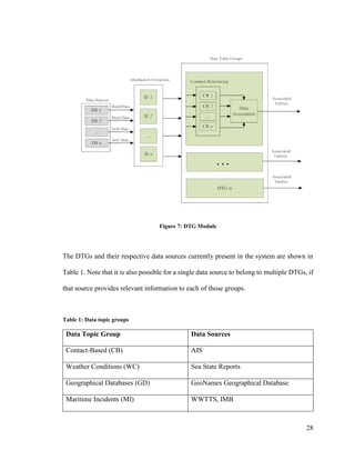
3.2.1 Data Topic Groups
This study proposes a grouping of data sources in the system according to the type
of information they provide. For instance, WWTTS and IMB provide incident reports of
very similar nature, and thus belong to the same group, namely, the Maritime Incidents
group. A detailed diagram of the DTG subcomponent is presented in Figure 7. This
subcomponent takes multiple data sources as input and is responsible for providing all the
information available on unique entities described by the input data sources.](https://image.slidesharecdn.com/14ada79c-c8c9-462e-aceb-00c958cdaf17-161228170344/85/Plachkov_Alex_2016_thesis-41-320.jpg)
![30
report, and produces the set, R, containing relevant response information extracted from
the report:
𝑹 = {𝒗𝒆𝒔𝒔𝒆𝒍𝑻𝒚𝒑𝒆, 𝑲, 𝒊𝒏𝒄𝒊𝒅𝒆𝒏𝒕𝑻𝒊𝒎𝒆, 𝒊𝒏𝒄𝒊𝒅𝒆𝒏𝒕𝑳𝒐𝒄𝒂𝒕𝒊𝒐𝒏} (1)
where K is the set of incident keywords discovered in the report.
The MI IE submodule makes use of the Natural Language Processing (NLP) technique
called Named-Entity Recognition (NER) in order to extract information from the textual
incident report and construct the set R. There is a lexicon constructed for each of the
elements in the set R.
3.2.2 Risk Features
Two of the above risk features, namely the Degree of Distress and the Regional
Hostility Metric from [12], are augmented to include risk factors derived from the data
sources belonging in the MI DTG. The conceptual definitions of the two risk features
remain as previously stated in Section 3.2.
3.2.2.1 Regional Hostility Metric
The Regional Hostility Metric of vessel x, RHM(x), is formally defined as:
(2)
where wMIP, wMIS, and wVPI are used to respectively weigh: (a) the significance of vessel x's
proximity to known maritime incidents, (b) the importance of the severity of the incidents
around the vicinity of the vessel, and (c) the pertinence of the nearby incidents to the vessel.](https://image.slidesharecdn.com/14ada79c-c8c9-462e-aceb-00c958cdaf17-161228170344/85/Plachkov_Alex_2016_thesis-44-320.jpg)
![34
Table 4: Vessel types and their corresponding category
Cargo Transport Tanker/Industrial Warship Small
Military
Vessel
Small
Transport/Utility
Bulk carrier Chemical tanker warship Coast guard
boat
Fishing trawler
Car carrier Heavy lift vessel Naval patrol
vessel
Japanese
harpoonists
Cargo ship Lpg tanker Militant anti-
whaling group
Carrier ship Mother vessel Skiff
Container ship Oil tanker Speed boat
Dry cargo vessel Product tanker Tug boat
General cargo
ship
Tanker Dredger
Livestock carrier Fishing vessel
Lng carrier vessel
Refrigerated
cargo ship
Merchant ship
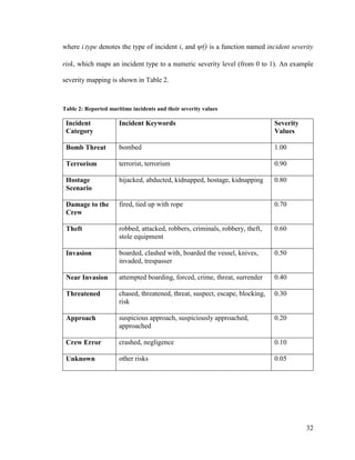
3.2.2.2 Degree of Distress
The Degree of Distress of vessel x, DoD(x), is augmented from [12] with another
distress factor, the Risk of Attack, that will be derived from textual information mined
directly from the semi-structured maritime incident reports; it is formally defined as:
(7)](https://image.slidesharecdn.com/14ada79c-c8c9-462e-aceb-00c958cdaf17-161228170344/85/Plachkov_Alex_2016_thesis-48-320.jpg)
![35
Where the integer values present a suggested weighing, and μRP(x), μRE(x), and μRF(x)
remain as previously defined as in [12] and μRA(x) is the probability that vessel x will be
attacked due to the category it belongs to (according to its vessel type). More formally,
μRA(x)is the square root of the conditional probability that x.category would be the subject
of a maritime incident I:
(8)
3.3 Performance Evaluation
As was discussed in Section 2.4, quantifying the effectiveness of an IF system is
still a burgeoning area in the fusion community. The prevalent theme in the IF quality
evaluation literature is that there is no commonly agreed-upon method and set of quality
measures that can be used to evaluate a general fusion system; this is largely because
quality is dependent on user objectives in a specific context [7] [60] [39] [61].
Recent attempts to quantify the IFE were [62] and [68], where the proposed metric
consists of three aspects: (1) the information gain, quantifying the aggregation level of
content provided by the data sources; (2) the information quality, which is a measure of
data characteristics such as timeliness and information confidence; and (3) the robustness
defined as the ability of the system to cope with real-world variation [68].
This research proposes a generic risk-aware IFE metric, capable of quantifying the
effectiveness of the HSIF process. Furthermore, an IFE evaluation from two perspectives
is formulated – from an instantaneous and from a gradual perspective. The typical
evaluation done in terms of comparing against ground truth values (computing Precision,
Recall, and F-measure) provides an overall (“averaged”) performance assessment;](https://image.slidesharecdn.com/14ada79c-c8c9-462e-aceb-00c958cdaf17-161228170344/85/Plachkov_Alex_2016_thesis-49-320.jpg)
![37
3.3.1 Instantaneous Information Fusion Effectiveness
As previously discussed, this research expands on the domain-agnostic
Information Gain (IG) and Information Quality (IQ) measures proposed in [62] and [68],
to formulate a risk-aware fusion effectiveness metric, whose building blocks are
presented in Figure 8.
Figure 8: Instantaneous information fusion effectiveness (i-IFE) hierarchy](https://image.slidesharecdn.com/14ada79c-c8c9-462e-aceb-00c958cdaf17-161228170344/85/Plachkov_Alex_2016_thesis-51-320.jpg)
![38
From a top-level perspective, the i-IFE metric is calculated as the product of IG and IQ;
furthermore, i-IFE 𝜖 [0, 1].
(9)
Table 5 presents commonly used symbols in the equations from the subsequent sections.
Table 5: Notations for i-IFE
Symbol Definition
S a maritime scenario; a static snapshot (of configurable time length) of
the assets present in a particular region
Sendtime denotes a scenario's end time
x a maritime vessel
i a maritime incident
NRn(x.loc) the set of nearest n incident reports to vessel x
NRr(x.loc) the set of nearest relevant incident reports to vessel x
NWn(x.loc) the set of nearest weather condition measurements to vessel x
ING(x) the set of nearest n incidents which report only general locations, or
more formally:
𝐼 𝑁𝐺(𝑥) = { 𝑖 𝜖 𝑁𝑅 𝑛(𝑥. 𝑙𝑜𝑐) ∶ 𝑖. 𝑙𝑜𝑐𝑆𝑝𝑒𝑐𝑖𝑓𝑖𝑐 = 𝑛𝑢𝑙𝑙}
A the set of attributes across all data sources belonging to a particular data
topic group that are contributing to the fusion process
O the set of distinct objects present in the data sources which belong to a
particular data topic group
W the set of all possible objects (in the environment being monitored)
DTGR data topic group relevance – a weight meant to quantify the relevance of
the DTG to the fusion objectives.](https://image.slidesharecdn.com/14ada79c-c8c9-462e-aceb-00c958cdaf17-161228170344/85/Plachkov_Alex_2016_thesis-52-320.jpg)
![43
3.3.1.2.1 Information Confidence
IC is based on several information quality measures, namely Reliability of
Information (ROI), Reliability of Source (ROS), Validity (V), and Completeness
(C); it is formally defined as their weighted sum:
(20)
The sum of all the weights must be unity. For this research, the weights were all equal: wC
= wV = wROI = wROS = ¼, however, as with Equations (10) and (19), this is kept
parameterizable according to the operator’s preferences.
A. Reliability
ROS and ROI values have been defined according to the US Military Standard 640
(MIL-STD-640) [62], which provides quantitative values for the otherwise qualitative
descriptions of the reliability levels of information and source of information found in the
NATO Standardized Agreement for Intelligence Reports – STANAG 2022. The need for
assessing ROS and ROI separately stems from the fact that information's quality is
instantaneous, whereas a source's quality is enduring (i.e., based on previous experience
with that information source) [7]. An unreliable source may provide a reliable piece of
information at a certain point in time; the converse is also true.
B. Validity
Validity is defined as the “degree of truthfulness” in information [38]. In the RMF, this
degree will be judged by adherence to the expected format of the attributes of the data in a
particular DTG:
(21)](https://image.slidesharecdn.com/14ada79c-c8c9-462e-aceb-00c958cdaf17-161228170344/85/Plachkov_Alex_2016_thesis-57-320.jpg)
![44
where the attributes for the CB and MI DTGs are ACB = AMI = {location, time, vessel type},
the attributes for WC are AWC = {location, time}, and the attribute for the GD DTG is AGD
= {location}. FC refers to format check, which returns unity if the attribute is in the correct
format, or zero otherwise. The format check of the coordinate returns unity if they are over
water, or zero if they are over land.
The overall Validity measure of the system is the weighted sum of the individual
Validity measures:
(22)
C. Completeness
The Completeness of a data source is broadly defined as the “proportion of missing
values” [60]. The authors in [69] expand on this notion by taking into account the total
information present in the real world. Completeness of a source then becomes a construct
which describes the amount of information provided by the source as compared to the total
amount of information present in the world (domain) which the source is describing. The
formalization is accomplished by introducing two dimensions of Completeness, namely
Coverage and Density.
The Completeness of a DTG (CDTG) is formalized as the product of the Coverage of
the DTG (CvDTG) and the Density of the DTG (dDTG):
(23)](https://image.slidesharecdn.com/14ada79c-c8c9-462e-aceb-00c958cdaf17-161228170344/85/Plachkov_Alex_2016_thesis-58-320.jpg)
![45
The overall Completeness measure of the system is the weighted sum of the individual
DTG Completeness measures:
(24)
a. Coverage
The Coverage of an information source is defined as the ratio of the number of
objects present in the source to the total number of possible objects in the world. This
notion is expanded in the system by applying the Coverage to a DTG (i.e., the Coverage is
a measure applied to all the data sources belonging to the DTG):
(25)
where O and W remain as previously defined in Table 5.
The authors in [69] point out that it is not always possible to have explicit
knowledge of W, and therefore, in such a case, the coverage of a source can be only
estimated by a domain expert (an SME).
b. Density
The Density of an information source quantifies how much data the source provides
for each of the objects described within it; it is thus a measure of the number of non-null
attributes the source provides. The notion of Density is expanded within this research by
applying it to a DTG. More formally:
(26)](https://image.slidesharecdn.com/14ada79c-c8c9-462e-aceb-00c958cdaf17-161228170344/85/Plachkov_Alex_2016_thesis-59-320.jpg)
![47
(28)
where t is the sorted collection of time stamps reported by vessel x in the scenario, x.t[1]
represents the first time stamp, and n is the number of time stamps reported by that same
vessel.
FITCB is the fuzzy variable whose crisp input is ITCB, and has the linguistic terms
CBRecent and CBOld.
The IT of the MI DTG, ITMI, is the average, across all vessels, of the average age
(in days) of each vessel’s n closest maritime incident reports to the scenario’s end time,
drawn from data sources belonging to the DTG:
(29)
where τMI is the MI’s temporal staleness point, and ITNRn(x) represents the timeliness of
the n nearest incident reports to vessel x, from the scenario’s end time, and is formally
defined as:
(30)
where x.t represents the last reported time by vessel x, and i.t represents the reported time
of incident i.](https://image.slidesharecdn.com/14ada79c-c8c9-462e-aceb-00c958cdaf17-161228170344/85/Plachkov_Alex_2016_thesis-61-320.jpg)
![49
The set of membership functions associated with the OIT fuzzy variable are OITRecent,
OITAcceptable, and OITOld.
Note that the GD DTG does not contribute to the OIT metric because the group only
contains data sources with static (i.e., time-invariant) information. Also, FITCB is chosen
to play a predominant role in the above rules due the fact that the CB DTG contains the
information most vital to the system; the latter’s capability to accurately detect risk vastly
deteriorates when there is only very scarce and untimely CB-related data.
3.3.2 Gradual Information Fusion Effectiveness
The g-IFE metric is calculated as the trimmed, or truncated mean of the set of i-IFE
values collected for each of the scenarios present in a region over a user-specified time
period. The trimmed mean is chosen due to its robustness in relation to outliers [70]. Outlier
i-IFE values (i.e., ones that are unusually high or low) are possible when the system first
starts due to the data transmission rates (e.g., a scenario has very little CB data due to the
CB transmission rates, but in reality, the region has many maritime entities); however, as
the system remains active over a period of time, the knowledge of the entities which are
present grows, and outlier i-IFEs are no longer expected.
(33)
(34)
where R is the region , E is the set of ordered i-IFEs, and 𝐸̅{0.20} is the 20% trimmed
mean of E.](https://image.slidesharecdn.com/14ada79c-c8c9-462e-aceb-00c958cdaf17-161228170344/85/Plachkov_Alex_2016_thesis-63-320.jpg)
![50
Since i-IFEs 𝜖 [0,1], from Equation (34) it follows that g-IFEs 𝜖 [0,1].
3.3.3 Robustness Analysis
As previously discussed, robustness is defined as the ability of a system to cope
with real-word variations [68]. Within the proposed HSIF system, robustness is judged via
Information Loss Tolerance (ILT) experiments and Use Case Coverage (UCC) analysis.
3.3.3.1 Information Loss Tolerance
An ILT analysis is done on the system by randomly dropping a defined percentage
of entities (e.g., incident information, weather condition measurements) and measuring the
new g-IFE values. These g-IFE values are then used to determine the effect this disturbance
has on the performance of the system.
In order to determine the ILT level, it is necessary to determine the disturbance
percentage the information loss has caused on the g-IFE metric:
(35)
where α represents the percentage gain (+) or loss (-) relative to g-IFE. The optimal case
is that α is equal to 0%, which occurs when the disturbance inserted into the system had no
effect on the g-IFE metric. Note that as previously discussed, g-IFE and g-IFE(InfoLoss)
are always positive values in the interval [0, 1].
The ILT can then be defined as follows:](https://image.slidesharecdn.com/14ada79c-c8c9-462e-aceb-00c958cdaf17-161228170344/85/Plachkov_Alex_2016_thesis-64-320.jpg)
![51
(36)
where β represents a threshold percentage of allowed g-IFE metric variation. If the
percentage disturbance caused to the g-IFE metric is under the threshold, then the metric
is said to be tolerant of the information loss [suggested β = 0.05 (i.e., 5%)].
3.3.3.2 Use Case Coverage
The second aspect of robustness is UCC – the ratio of the total number of use cases in
which the system can be run whilst providing useful L2 fusion capabilities (i.e., the core
functionality is still available) to the total number of possible ways to run the system. If
there are X information sources, then there are 2X
use cases (i.e., all possible combinations
of the sources). The system’s UCC then can be determined as the total number of cases
(data source combinations) which would render the system useful divided by the total
number of possible combinations:
(37)
where D is the set of data sources used by the system, 2D
is the powerset of D, δ() is a
function that identifies the number of useful elements in the powerset (in the RMF context
– number of useful use cases).](https://image.slidesharecdn.com/14ada79c-c8c9-462e-aceb-00c958cdaf17-161228170344/85/Plachkov_Alex_2016_thesis-65-320.jpg)
![52
3.3.4 Profitability Analysis
Profitability analysis can be conducted on the g-IFE metric by starting with a
baseline configuration (e.g., system running with AIS data only) and calculating the g-IFE
percent gain for another configuration (e.g., adding a new data source). This analysis will
demonstrate the underlying merit provided by the additional sources.
(38)
where ∏ (𝐴)𝐵 denotes the profitability – g-IFE percent gain or loss – achieved by adding a
set of sources A into the system, given a set, B, of baseline sources. Note that it is possible
to have infinite profit, but not infinite loss, as g-IFE can never be negative.
3.4 Chapter Summary
This chapter proposed a new L2 SA soft-data augmented extension to a recently
proposed RMF [12], for the purpose of proactively identifying vessels which may
fall in distress. A new L2-based IFE metric is proposed for the purpose of
evaluating instantaneous and gradual performance of the fusion process of the
system. Further presented were two types of analyses, Robustness and Profitability,
which can be performed on the basis of the IFE metric, for the purpose of: (1)
gauging the system’s ability to cope with real-world variation and (2) determining
the merit provided by different data sources, respectively.](https://image.slidesharecdn.com/14ada79c-c8c9-462e-aceb-00c958cdaf17-161228170344/85/Plachkov_Alex_2016_thesis-66-320.jpg)
![62
4.2.2 Asset Selection Module
The ASM is responsible for selecting which response assets will be carrying out
the mission, based on the mission requirements (which define what specific types of assets
are required for each situation, as well as their associated onboard sensors). The module
provides a designated search area for each asset. Asset search area designation is optimized
with the popular Non-dominated Sorting Genetic Algorithm II (NSGA-II) [71]. This
algorithm is used for EMOO to produce a set of spread non-dominated candidate solutions
with varying degrees of mission latency, cost, response area gap sizes, and levels to which
they meet mission requirements.
4.2.2.1 Response Encoding
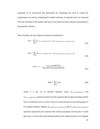
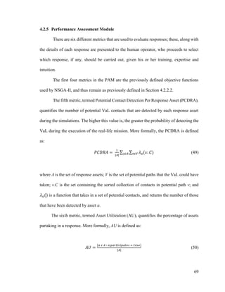
Whenever an incident is detected, a response grid pertaining to that incident is
generated and broken down into a square grid. Each cell is a square, which is entirely
enclosed within the sweep area of the smallest-sweeping sensor of any of the selected
assets. Figure 11 presents an example response grid, with three (coloured) subgrids, each
of which is assigned to a response asset. The grid also shows two continuous gaps in
coverage (in white).
Figure 11: Example response grid with three designated subgrids](https://image.slidesharecdn.com/14ada79c-c8c9-462e-aceb-00c958cdaf17-161228170344/85/Plachkov_Alex_2016_thesis-76-320.jpg)
![71
Chapter 5. Experimentation
This section presents the experiments conducted for the purpose of empirical
evaluation on the L2 and L3 methodologies described in Chapter 3 and Chapter 4.
5.1 Situational Assessment Experiments
Two regions are selected for the purpose of evaluating the risk-aware HSIF model,
and the practicability of the IFE metric. The first experiment is situated in the
Malaysia/Singapore region, whereas the second is set in the Bangladesh region. The former
region is a hotspot for maritime piracy, with an ever-increasing number of incidents16
, as
reported by the IMB. In contrast, the latter region was selected due to its relatively placid
nature.
5.1.1 Experimental Configuration
This section lays out the configuration of the system that was used for the
maritime experiments.
5.1.1.1 Coverage
The Coverage measures for CB, MI, and GD for these experiments are non-
computable, since it is not possible to be cognizant of all the entities that are present in the
maritime environment being described by the data sources (there is no access to ‘ground
truth’); the actual Coverage values are thus provided by domain experts, as is typically
done in such a case [69]. The values with which the system was run are as follows: CvCB
= CvMI = 0.6. These values were selected through SME feedback from Larus Technologies
16
http://maritime-executive.com/article/pirates-hijack-tanker-off-malaysian-coast](https://image.slidesharecdn.com/14ada79c-c8c9-462e-aceb-00c958cdaf17-161228170344/85/Plachkov_Alex_2016_thesis-85-320.jpg)
![72
and IMB, respectively. Since the only data source present in the WC DTG was a simulated
one, this DTG’s Coverage value was set to be CvWC = 1.0. Furthermore, CvGD was
estimated to be 1.0, since the only data source currently present in the group is GeoNames
DB, a comprehensive database with over 10 million geographical names.
5.1.1.2 Overall Information Timeliness
The fuzzy linguistic terms of the OIT sub-component of the i-IFE metric were defined
according to maritime subject matter expertise (as provided by Larus Technologies), and
were constructed as follows:
• CBRecent(trapezoidal, A = 0, B = 0, C = 600, D = 1200), and
CBOld(trapezoidal, A = 600, B = 1200, C = ∞, D = ∞); units are in seconds.
• MIRecent (trapezoidal, A = 0, B = 0, C = 500, D = 732), and
MIOld (trapezoidal, A = 500, B = 732, C = ∞, D = ∞); units are in days.
• WCRecent (trapezoidal, A = 0, B = 0, C = 1, D = 2), and
WCOld (trapezoidal, A = 1, B = 2, C = ∞, D = ∞); units are in hours.
• OITRecent (triangular, A = 0.5, B = 1, C = 1.5),
OITAcceptable(triangular, A = 0, B = 0.5, C = 1),
and OITOld (triangular, A = 0.5, B = 0, C = 1.5)
The reader may notice that the OITRecent’s parameter C is set to 1.5, and that the
OITOld’s parameter A is set to -0.5; however, the range of values that the crisp OIT output
can take is in the region [0,1], as determined by the respective centroids of the OITRecent
and OITOld fuzzy linguistic terms.](https://image.slidesharecdn.com/14ada79c-c8c9-462e-aceb-00c958cdaf17-161228170344/85/Plachkov_Alex_2016_thesis-86-320.jpg)
![115
Chapter 6. Concluding Remarks
This study focused on extending an existing RMF’s L2 and L3 fusion capabilities
through the inclusion of soft data for the purpose of increased SA and improved CoA
generation. At the L2 level, the RMF’s (SA) risk model was enhanced via the augmentation
of two risk features, the Degree of Distress and the Regional Hostility Metric, with the
injection of information derived from soft maritime incident reports. At the L3 level, the
RMF’s capabilities were enhanced by proposing a new soft data-augmented CoA
subsystem architecture.
Performance metrics were introduced on both the L2 and L3 levels, and used to
quantify the value brought to the system by the inclusion of this type of data. The
experimental analysis conducted as part of this research demonstrated how the injection of
the soft data into the two fusion levels yielded higher mission-specific measures of
performance (as defined at each respective level). To the best of my knowledge, this work
is the first one to apply soft data to automated CoA generation and performance evaluation
in the maritime domain.
Parts of this work has been published in the form of Association for Computing
Machinery (ACM) and Institute of Electrical and Electronics Engineers (IEEE) conference
proceedings in [72] and [73], respectively, as well as orally presented at a Canadian
Tracking and Fusion Group (CTFG) workshop18
.
18
http://www.ctfg.ca/](https://image.slidesharecdn.com/14ada79c-c8c9-462e-aceb-00c958cdaf17-161228170344/85/Plachkov_Alex_2016_thesis-129-320.jpg)
![117
Artificial Neural Network (ANN). Further automated analysis of the soft data could be
performed so as to judge historical mission success levels, and attempt to identify which
response elements cause missions to fail. Such response elements could then become
chromosome constraints in the NSGA-II when generating suitable CoAs. For the purposes
of generating suitable responses adhering to more than four mission objectives, a new
category of optimization algorithms, Many-Objective Evolutionary Algorithms (MaOEAs)
[75], can also be explored.](https://image.slidesharecdn.com/14ada79c-c8c9-462e-aceb-00c958cdaf17-161228170344/85/Plachkov_Alex_2016_thesis-131-320.jpg)
![118
References
[1] R. Abielmona, "Tackling big data in maritime domain awareness," Vanguard, pp.
42-43, August-September 2013.
[2] U.S. National Concept of Operations for Maritime Domain Awareness, 2007.
[3] E. Blasch and S. Plano, "DFIG level 5 (user refinement) issues supporting
situational assessment reasoning," in Information Fusion, 2005 8th International
Conference on, 2005.
[4] E. Blasch, I. Kadar, J. Salerno, M. M. Kokar, G. M. Powell, D. D. Corkill and E.
H. Ruspini, "Issues and Challenges in Situation Assessment (Level 2 Fusion),"
Journal of Advances in Information Fusion, vol. 1, pp. 122-139, December 2006.
[5] R. Falcon, R. Abielmona and E. Blasch, "Behavioral learning of vessel types with
fuzzy-rough decision trees," in Information Fusion (FUSION), 2014 17th
International Conference on, 2014.
[6] J. C. Rimland and J. Llinas, "Network and infrastructure considerations for hard
and soft information fusion processes," in Information Fusion (FUSION), 2012
15th International Conference on, 2012.
[7] A.-L. Jousselme, A.-C. Boury-Brisset, B. Debaque and D. Prevost,
"Characterization of hard and soft sources of information: A practical
illustration," in Information Fusion (FUSION), 2014 17th International
Conference on, 2014.](https://image.slidesharecdn.com/14ada79c-c8c9-462e-aceb-00c958cdaf17-161228170344/85/Plachkov_Alex_2016_thesis-132-320.jpg)
![119
[8] G. A. Gross, D. R. Schlegel, J. J. Corso, J. Llinas, R. Nagi, S. C. Shapiro and
others, "Systemic test and evaluation of a hard+ soft information fusion
framework: Challenges and current approaches," in Information Fusion
(FUSION), 2014 17th International Conference on, 2014.
[9] D. L. Hall, M. McNeese, J. Llinas and T. Mullen, "A framework for dynamic
hard/soft fusion," in Information Fusion, 2008 11th International Conference on,
2008.
[10] A. H. Razavi, D. Inkpen, R. Falcon and R. Abielmona, "Textual risk mining for
maritime situational awareness," in 2014 IEEE International Inter-Disciplinary
Conference on Cognitive Methods in Situation Awareness and Decision Support
(CogSIMA), 2014.
[11] R. Falcon, R. Abielmona and A. Nayak, "An Evolving Risk Management
Framework for Wireless Sensor Networks," in Proceedings of the 2011 IEEE Int'l
Conference on Computational Intelligence for Measurement Systems and
Applications (CIMSA), 2011.
[12] R. Falcon and R. Abielmona, "A Response-Aware Risk Management Framework
for Search-and-Rescue Operations," in 2012 IEEE Congress on Evolutionary
Computation (CEC), 2012.
[13] C. K. Ioannis Chapsos, "Strengthening maritime security through cooperation,"
IOS Press, vol. 122, 2015.
[14] ISO, "Risk management: Principles and Guidelines," International Organization
for Standardization, no. 31000, 2009.](https://image.slidesharecdn.com/14ada79c-c8c9-462e-aceb-00c958cdaf17-161228170344/85/Plachkov_Alex_2016_thesis-133-320.jpg)
![120
[15] P. H. Foo and G. W. Ng, "High-level Information Fusion: An Overview.,"
Journal of Advances in Information Fusion, vol. 8, no. 1, pp. 33-72, 2013.
[16] J. Montewka, S. Ehlers, F. Goerlandt, T. Hinz, K. Tabri and P. Kujala, "A
framework for risk assessment for maritime transportation systems--A case study
for open sea collisions involving RoPax vessels," Reliability Engineering &
System Safety, vol. 124, pp. 142-157, 2014.
[17] J. R. W. Merrick, J. R. Van Dorp and V. Dinesh, "Assessing Uncertainty in
Simulation-Based Maritime Risk Assessment," Risk Analysis, vol. 25, no. 3, pp.
731-743, 2005.
[18] X. Tan, Y. Zhang, X. Cui and H. Xi, "Using hidden markov models to evaluate
the real-time risks of network," in Knowledge Acquisition and Modeling
Workshop, 2008. KAM Workshop 2008. IEEE International Symposium on, 2008.
[19] K. Haslum and A. Arnes, "Real-time Risk Assessment using Continuous-time
Hidden Markov Models," in Proceedings of Int’l Conference on Computational
Intelligence and Security, 2006.
[20] A. Mazaheri, J. Montewka, J. Nisula and P. Kujala, "Usability of accident and
incident reports for evidence-based risk modeling--A case study on ship
grounding reports," Safety science, vol. 76, pp. 202-214, 2015.
[21] R. Falcon, R. Abielmona and S. Billings, "Risk-driven intent assessment and
response generation in maritime surveillance operations," in Cognitive Methods in
Situation Awareness and Decision Support (CogSIMA), 2015 IEEE International
Inter-Disciplinary Conference on, 2015.](https://image.slidesharecdn.com/14ada79c-c8c9-462e-aceb-00c958cdaf17-161228170344/85/Plachkov_Alex_2016_thesis-134-320.jpg)
![121
[22] N. A. Bomberger, B. J. Rhodes, M. Seibert and A. M. Waxman, "Associative
learning of vessel motion patterns for maritime situation awareness," in
Information Fusion, 2006 9th International Conference on, 2006.
[23] B. J. Rhodes, N. A. Bomberger, M. Seibert and A. M. Waxman, "Maritime
situation monitoring and awareness using learning mechanisms," in Military
Communications Conference, 2005. MILCOM 2005. IEEE, 2005.
[24] R. Laxhammar, "Artificial intelligence for situation assessment," 2007.
[25] M. Guerriero, P. Willett, S. Coraluppi and C. Carthel, "Radar/AIS data fusion and
SAR tasking for maritime surveillance," in Information Fusion, 2008 11th
International Conference on, 2008.
[26] L. Snidaro, I. Visentini and K. Bryan, "Fusing uncertain knowledge and evidence
for maritime situational awareness via Markov Logic Networks," Information
Fusion, vol. 21, pp. 159-172, 2015.
[27] F. Johansson and G. Falkman, "Detection of vessel anomalies-a Bayesian network
approach," in Intelligent Sensors, Sensor Networks and Information, 2007. ISSNIP
2007. 3rd International Conference on, 2007.
[28] R. Laxhammar, G. Falkman and E. Sviestins, "Anomaly detection in sea traffic-a
comparison of the Gaussian mixture model and the kernel density estimator," in
Information Fusion, 2009. FUSION'09. 12th International Conference on, 2009.
[29] R. N. Carvalho, R. Haberlin, P. C. G. Costa, K. B. Laskey and K.-C. Chang,
"Modeling a probabilistic ontology for maritime domain awareness," in](https://image.slidesharecdn.com/14ada79c-c8c9-462e-aceb-00c958cdaf17-161228170344/85/Plachkov_Alex_2016_thesis-135-320.jpg)
![122
Information Fusion (FUSION), 2011 Proceedings of the 14th International
Conference on, 2011.
[30] A. Bouejla, X. Chaze, F. Guarnieri and A. Napoli, "A Bayesian network to
manage risks of maritime piracy against offshore oil fields," Safety Science, vol.
68, pp. 222-230, 2014.
[31] H. Shao, N. Japkowicz, R. Abielmona and R. Falcon, "Vessel track correlation
and association using fuzzy logic and echo state networks," in Evolutionary
Computation (CEC), 2014 IEEE Congress on, 2014.
[32] N. Le Guillarme and X. Lerouvreur, "Unsupervised extraction of knowledge from
S-AIS data for maritime situational awareness," in Information Fusion (FUSION),
2013 16th International Conference on, 2013.
[33] G. Pallotta, M. Vespe and K. Bryan, "Vessel pattern knowledge discovery from
AIS data: A framework for anomaly detection and route prediction," Entropy, vol.
15, no. 6, pp. 2218-2245, 2013.
[34] C.-H. Chen, L. P. Khoo, Y. T. Chong and X. F. Yin, "Knowledge discovery using
genetic algorithm for maritime situational awareness," Expert Systems with
Applications, vol. 41, no. 6, pp. 2742-2753, 2014.
[35] L. Vanneschi, M. Castelli, E. Costa, A. Re, H. Vaz, V. Lobo and P. Urbano,
"Improving Maritime Awareness with Semantic Genetic Programming and Linear
Scaling: Prediction of Vessels Position Based on AIS Data," in Applications of
Evolutionary Computation, Springer, 2015, pp. 732-744.](https://image.slidesharecdn.com/14ada79c-c8c9-462e-aceb-00c958cdaf17-161228170344/85/Plachkov_Alex_2016_thesis-136-320.jpg)
![123
[36] M. Riveiro and G. Falkman, "The role of visualization and interaction in maritime
anomaly detection," in IS&T/SPIE Electronic Imaging, 2011.
[37] M. Riveiro, G. Falkman and T. Ziemke, "Improving maritime anomaly detection
and situation awareness through interactive visualization," in Information Fusion,
2008 11th International Conference on, 2008.
[38] E. Blasch, E. Bosse and D. A. Lambert, High-Level Information Fusion
Management and Systems Design, Artech House, 2012.
[39] G. L. Rogova and E. Bosse, "Information quality in information fusion," in
Information Fusion (FUSION), 2010 13th Conference on, 2010.
[40] J. Llinas, "Information Fusion Process Design Issues for Hard and Soft
Information: Developing an Initial Prototype," in Intelligent Methods for Cyber
Warfare, Springer, 2015, pp. 129-149.
[41] A. Preece, D. Pizzocaro, D. Braines, D. Mott, G. de Mel and T. Pham,
"Integrating hard and soft information sources for D2D using controlled natural
language," in Information Fusion (FUSION), 2012 15th International Conference
on, 2012.
[42] M. P. Jenkins, G. A. Gross, A. M. Bisantz and R. Nagi, "Towards context aware
data fusion: Modeling and integration of situationally qualified human
observations to manage uncertainty in a hard+ soft fusion process," Information
Fusion , vol. 21, no. 0, pp. 130-144, 2015.](https://image.slidesharecdn.com/14ada79c-c8c9-462e-aceb-00c958cdaf17-161228170344/85/Plachkov_Alex_2016_thesis-137-320.jpg)
![124
[43] D. McMaster, R. Nagi and K. Sambhoos, "Temporal alignment in soft
information processing," in Information Fusion (FUSION), 2011 Proceedings of
the 14th International Conference on, 2011.
[44] G. A. Gross, R. Nagi and others, "Test and evaluation of data association
algorithms in hard+ soft data fusion," in Information Fusion (FUSION), 2014 17th
International Conference on, 2014.
[45] J. Gómez-Romero, M. A. Serrano, J. García, J. M. Molina and G. Rogova,
"Context-based multi-level information fusion for harbor surveillance,"
Information Fusion , vol. 21, no. 0, pp. 173-186, 2015.
[46] J. G. a. J. L. L. Snidaro, "Context-based Information Fusion: A Survey and
Discussion," Information Fusion, vol. 25, pp. 16-31, 2015.
[47] A.-C. Boury-Brisset, "Ontology-based approach for information fusion," in
Information Fusion, 2003. Proceedings of the Sixth International Conference of,
2003.
[48] M. M. Kokar, C. J. Matheus and K. Baclawski, "Ontology-based situation
awareness," Information Fusion , vol. 10, no. 1, pp. 83-98, 2009.
[49] B. Khaleghi, A. Khamis, F. O. Karray and S. N. Razavi, "Multisensor data fusion:
A review of the state-of-the-art," Information Fusion, vol. 14, no. 1, pp. 28-44,
2013.
[50] P. Smets, "Imperfect information: Imprecision and uncertainty," in Uncertainty
Management in Information Systems, Springer, 1997, pp. 225-254.](https://image.slidesharecdn.com/14ada79c-c8c9-462e-aceb-00c958cdaf17-161228170344/85/Plachkov_Alex_2016_thesis-138-320.jpg)
![125
[51] K. J. Laskey and K. B. Laskey, "Uncertainty Reasoning for the World Wide Web:
Report on the URW3-XG Incubator Group.," in URSW, 2008.
[52] K. Premaratne, M. N. Murthi, J. Zhang, M. Scheutz and P. H. Bauer, "A
Dempster-Shafer theoretic conditional approach to evidence updating for fusion
of hard and soft data," in Information Fusion, 2009. FUSION'09. 12th
International Conference on, 2009.
[53] S. Fossier, C. Laudy and F. Pichon, "Managing uncertainty in conceptual graph-
based soft information fusion," in Information Fusion (FUSION), 2013 16th
International Conference on, 2013.
[54] D. Stampouli, M. Brown and G. Powell, "Fusion of soft information using TBM,"
in Information Fusion (FUSION), 2010 13th Conference on, 2010.
[55] G. Gross, R. Nagi and K. Sambhoos, "A fuzzy graph matching approach in
intelligence analysis and maintenance of continuous situational awareness,"
Information Fusion, vol. 18, pp. 43-61, 2014.
[56] B. Khaleghi, A. Khamis and F. Karray, "Random finite set theoretic based
soft/hard data fusion with application for target tracking," in Multisensor Fusion
and Integration for Intelligent Systems (MFI), 2010 IEEE Conference on, 2010.
[57] M. Liggins II, D. Hall and J. Llinas, Handbook of multisensor data fusion: theory
and practice, CRC press, 2008.
[58] J. L. Graham, D. L. Hall and J. Rimland, "A COIN-inspired synthetic dataset for
qualitative evaluation of hard and soft fusion systems," in Information Fusion
(FUSION), 2011 Proceedings of the 14th International Conference on, 2011.](https://image.slidesharecdn.com/14ada79c-c8c9-462e-aceb-00c958cdaf17-161228170344/85/Plachkov_Alex_2016_thesis-139-320.jpg)
![126
[59] D. L. Hall, J. Graham, L. D. More and J. C. Rimland, "Test and evaluation of
soft/hard information fusion systems: A test environment, methodology and initial
data sets," in Information Fusion (FUSION), 2010 13th Conference on, 2010.
[60] I.-G. Todoran, L. Lecornu, A. Khenchaf and J.-M. Le Caillec, "Information
quality evaluation in fusion systems," in Information Fusion (FUSION), 2013
16th International Conference on, 2013.
[61] E. Blasch, K. B. Laskey, A.-L. Jousselme, V. Dragos, P. C. G. Costa and J.
Dezert, "URREF reliability versus credibility in information fusion (STANAG
2511)," in Information Fusion (FUSION), 2013 16th International Conference on,
2013.
[62] E. P. Blasch, R. Breton and P. Valin, "Information fusion measures of
effectiveness (MOE) for decision support," in SPIE Defense, Security, and
Sensing, 2011.
[63] D. L. Hall, M. D. McNeese, D. B. Hellar, B. J. Panulla and W. Shumaker, "A
cyber infrastructure for evaluating the performance of human centered fusion," in
Information Fusion, 2009. FUSION'09. 12th International Conference on, 2009.
[64] P. C. G. Costa, K. B. Laskey, E. Blasch and A.-L. Jousselme, "Towards unbiased
evaluation of uncertainty reasoning: the URREF ontology," in Information Fusion
(FUSION), 2012 15th International Conference on, 2012.
[65] E. Blasch, A. Josang, J. Dezert, P. C. G. Costa and A.-L. Jousselme, "URREF
self-confidence in information fusion trust," in Information Fusion (FUSION),
2014 17th International Conference on, 2014.](https://image.slidesharecdn.com/14ada79c-c8c9-462e-aceb-00c958cdaf17-161228170344/85/Plachkov_Alex_2016_thesis-140-320.jpg)
![127
[66] A. M. S. Authority, "National Search and Rescue Manual," 6 2014. [Online].
Available: https://natsar.amsa.gov.au/documents/NATSAR-
Manual/Australian%20National%20SAR%20Manual%20June%202014%20FIN
AL.pdf. [Accessed 12 07 2016].
[67] D. Timmins, "Canadian Coast Guard National Search and Rescue Manual," 6
2000. [Online]. Available: http://loki.cgc.gc.ca/cansarp/sarmanuals/nsm.pdf.
[Accessed 12 07 2016].
[68] E. Blasch, P. Valin and E. Bosse, "Measures of effectiveness for high-level
fusion," in 13th Conference on Information Fusion ({FUSION}), 2010.
[69] F. Naumann and J. C. Freytag, "Completeness of information sources," in
Proceedings of the International Workshop on Data Quality in Cooperative
Information Systems (DQCIS ‘03), 2003.
[70] P. Paatero, "Least squares formulation of robust non-negative factor analysis,"
Chemometrics and intelligent laboratory systems, vol. 37, no. 1, pp. 23-35, 1997.
[71] K. Deb, A. Pratap, S. Agarwal and T. Meyarivan, "A fast and elitist
multiobjective genetic algorithm: NSGA-II," IEEE transactions on evolutionary
computation, vol. 6, no. 2, pp. 182-197, 2002.
[72] A. Plachkov, R. Abielmona, M. Harb, R. Falcon, D. Inkpen, V. Groza and E.
Petriu, "Automatic Course of Action Generation using Soft Data for Maritime
Domain Awareness," in Proceedings of the 2016 on Genetic and Evolutionary
Computation Conference Companion, Denver, 2016.](https://image.slidesharecdn.com/14ada79c-c8c9-462e-aceb-00c958cdaf17-161228170344/85/Plachkov_Alex_2016_thesis-141-320.jpg)
![128
[73] R. Falcon, R. Abielmona, S. Billings, A. Plachkov and H. Abbass, "Risk
management with hard-soft data fusion in maritime domain awareness," in
Computational Intelligence for Security and Defense Applications (CISDA), 2014
Seventh IEEE Symposium on, 2014.
[74] J. Li, B. Li, K. Tang and X. Yao, "Many-objective evolutionary algorithms: A
survey," ACM Computing Surveys (CSUR), vol. 48, no. 1, p. 13, 2015.
[75] J. Llinas, S. G. Dastidar, C. Bowman and K. Sambhoos, "Achieving "Fairness" in
Data Fusion Performance Evaluation Development," 2006.](https://image.slidesharecdn.com/14ada79c-c8c9-462e-aceb-00c958cdaf17-161228170344/85/Plachkov_Alex_2016_thesis-142-320.jpg)


