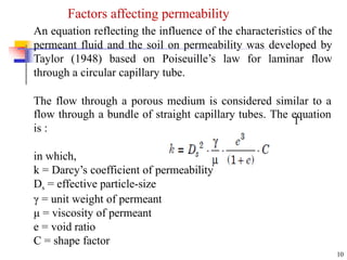
The document discusses permeability in porous materials, defining it as a property that allows water flow through soil. It outlines the significance of studying permeability for various engineering applications, including soil settlement, seepage in dams, and groundwater flow, while detailing Darcy's Law and factors affecting permeability such as grain size, temperature, and saturation. Additionally, it examines seepage forces, laboratory tests for permeability determination, flow net concepts, and piping phenomena related to soil and water interaction.


![[Vx + (Vx/x) dz dy] + [Vz + (Vz/z)
dx dy]
- [Vx dz dy + Vz dx dy ] = 0
30
Or Vx/x + Vz/z = 0
From Darcy’s Law Vx = Kx ix = Kx (h/x) & Vz = Kz iz =
= Kz (h/z)
For isotropic soil Kx = kz
2h/2
x + 2h/2
z = 0
known as Continuity Equation.
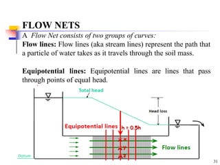
The flow net which consists of two sets of curves –
a series of flow lines and of equil-potential lines–is
obtained merely as a solution to the Laplace’s
equation.](https://image.slidesharecdn.com/permeabilitynotes-250103112622-7c3046d1/85/Permeability-notes-for-geotechnical-engineering-pptx-30-320.jpg)


![Geotechnical Engineering-I [Lec #23: Soil Permeability]](https://cdn.slidesharecdn.com/ss_thumbnails/23-180924141141-thumbnail.jpg?width=640&height=640&fit=bounds)


