Download to read offline
![International Journal of Information Sciences and Techniques (IJIST) Vol.3, No.6, November 2013
PERFORMANCE ANALYSIS OF NEURAL NETWORK
MODELS FOR OXAZOLINES AND OXAZOLES
DERIVATIVES DESCRIPTOR DATASET
Doreswamy and Chanabasayya .M. Vastrad
Department of Computer Science Mangalore University , Mangalagangotri-574 199,
Karnataka, India
ABSTRACT
Neural networks have been used successfully to a broad range of areas such as business, data mining, drug
discovery and biology. In medicine, neural networks have been applied widely in medical diagnosis,
detection and evaluation of new drugs and treatment cost estimation. In addition, neural networks have
begin practice in data mining strategies for the aim of prediction, knowledge discovery. This paper will
present the application of neural networks for the prediction and analysis of antitubercular activity of
Oxazolines and Oxazoles derivatives. This study presents techniques based on the development of Single
hidden layer neural network (SHLFFNN), Gradient Descent Back propagation neural network (GDBPNN),
Gradient Descent Back propagation with momentum neural network (GDBPMNN), Back propagation with
Weight decay neural network (BPWDNN) and Quantile regression neural network (QRNN) of artificial
neural network (ANN) models Here, we comparatively evaluate the performance of five neural network
techniques. The evaluation of the efficiency of each model by ways of benchmark experiments is an
accepted application. Cross-validation and resampling techniques are commonly used to derive point
estimates of the performances which are compared to identify methods with good properties. Predictive
accuracy was evaluated using the root mean squared error (RMSE), Coefficient determination( ܴଶ ), mean
absolute error(MAE), mean percentage error(MPE) and relative square error(RSE). We found that all five
neural network models were able to produce feasible models. QRNN model is outperforms with all
statistical tests amongst other four models.
KEYWORDS
Artificial neural network, Quantitative structure activity relationship, Feed forward neural network, back
propagation neural network
1. INTRODUCTION
The use of artificial neural networks (ANNs) in the area of drug discovery and optimization of
the dosage forms has become a topic of analysis in the pharmaceutical literature [1-5]. Compared
with linear modelling techniques, such as Multi linear regression (MLR) and Partial least squares
(PLS) , ANNs show better as a modelling technique for molecular descriptor data sets showing
non-linear conjunction, and thus for both data fitting and prediction strengths [6]. Artificial
neural network (ANN) is a vastly simplified model of the form of a biological network[7] .The
fundamental processing element of ANN is an artificial neuron (or commonly a neuron). A
DOI : 10.5121/ijist.2013.3601
1](https://image.slidesharecdn.com/performanceanalysisofneuralnetworkmodelsforoxazolinesandoxazolesderivativesdescriptordataset-131207023119-phpapp02/75/Performance-analysis-of-neural-network-models-for-oxazolines-and-oxazoles-derivatives-descriptor-dataset-1-2048.jpg)
![International Journal of Information Sciences and Techniques (IJIST) Vol.3, No.6, November 2013
biological neuron accepts inputs from other sources, integrate them, carry out generally a
nonlinear process on the result, and then outputs the last result [8]. The fundamental benefit of
ANN is that it does not use any mathematical model because ANN learns from data sets and
identifies patterns in a sequence of input and output data without any previous assumptions about
their type and interrelations [7]. ANN eliminates the drawbacks of the classical ways by
extracting the wanted information using the input data. Executing ANN to a system uses enough
input and output data in place of a mathematical equation[9]. ANN is a good alternative to
common empirical modelling based on linear regressions [10].
ANNs are known to be a powerful methodology to simulate various non-linear systems and have
been applied to numerous applications of large complexity in many field including
pharmaceutical research, engineering and medicinal chemistry. The promising uses of ANN
approaches in the pharmaceutical sciences are widespread. ANNs were also widely used in drug
discovery, especially in QSAR studies. QSAR is a mathematical connection between the
chemical’s quantitative molecular descriptors and its inhibitory activities [11-12]
Five Different types of neural network models have been developed for the development of
efficient antitubercular activity predicting models. Those models are Single hidden layer feed
forward neural network (SHLFNN)[13],Gradient Descent Back propagation neural network
(GDBPNN)[14,24], Gradient Descent Back propagation with momentum neural network
(GDBPMNN)[15-16],Back
propagation
with
Weight
decay
neural
network
(BPWDNN)[17],Quantile regression neural network (QRNN) [18].
The purpose of this research work and research publication is to assign five distinct neural
network models to the prediction of antitubercular activities of Oxazolines and Oxazoles
derivatives descriptor dataset. Method and along with estimate and asses their performances with
regard to their predicting ability. One of the goals of this scientific research project is to show
how distinct neural network models can be used in predicting antitubercular activities of
Oxazolines and Oxazoles derivatives descriptor dataset. It again involves inducing the best model
in terms of the least errors produced in the graphical study describing the actual and predicted
antitubercular activities.
2. MATERIALS AND ALGORITHAMS
2.1 The Data Set
The molecular descriptors of 100 Oxazolines and Oxazoles derivatives [19-20] based H37Rv
inhibitors analyzed. These molecular descriptors are produced using Padel-Descriptor tool [21].
The dataset includes a different set of molecular descriptors with a broad range of inhibitory
activities versus H37Rv. This molecular descriptor data set includes 100 observations with 234
descriptors. Before modelling, the dataset is ranged.
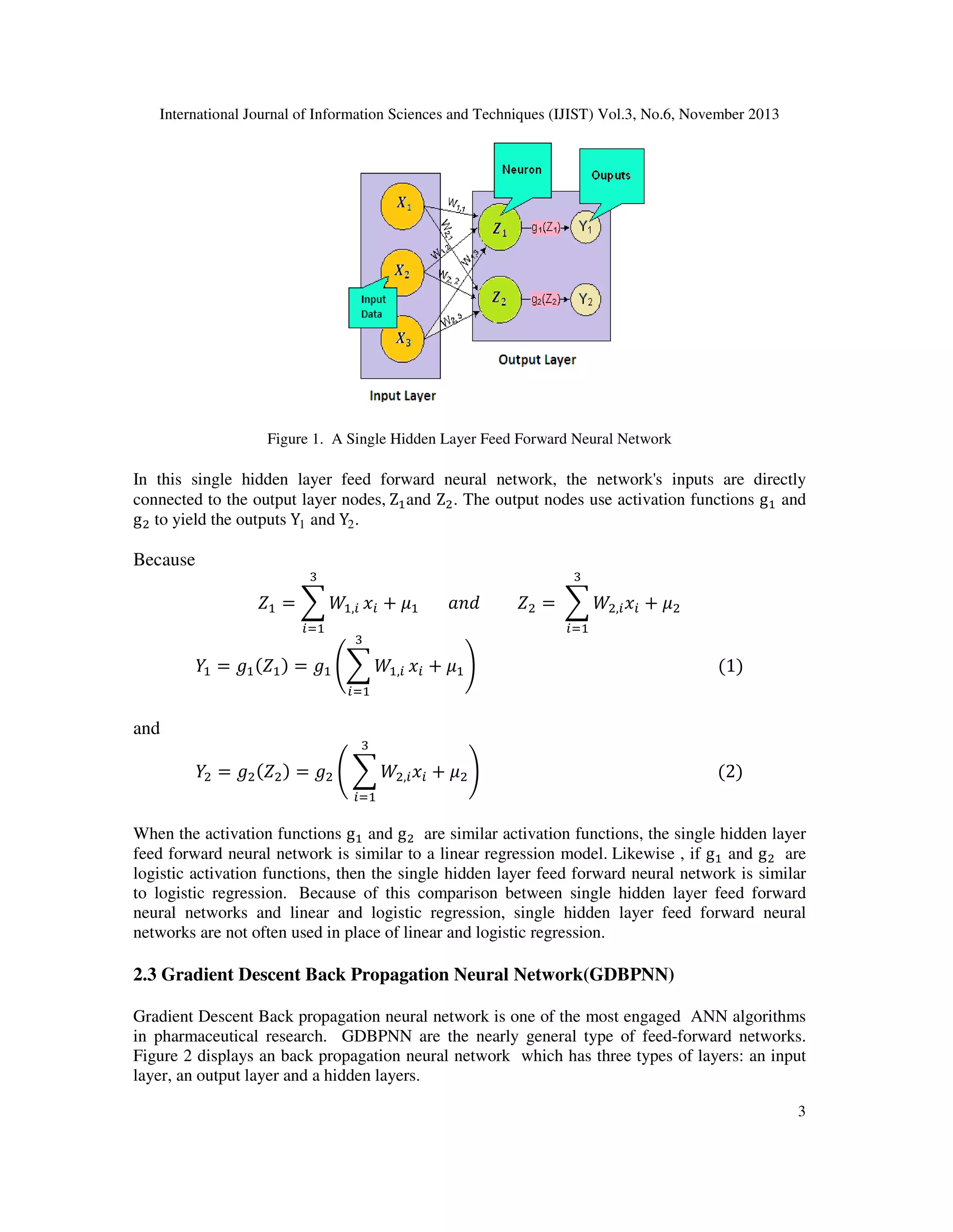
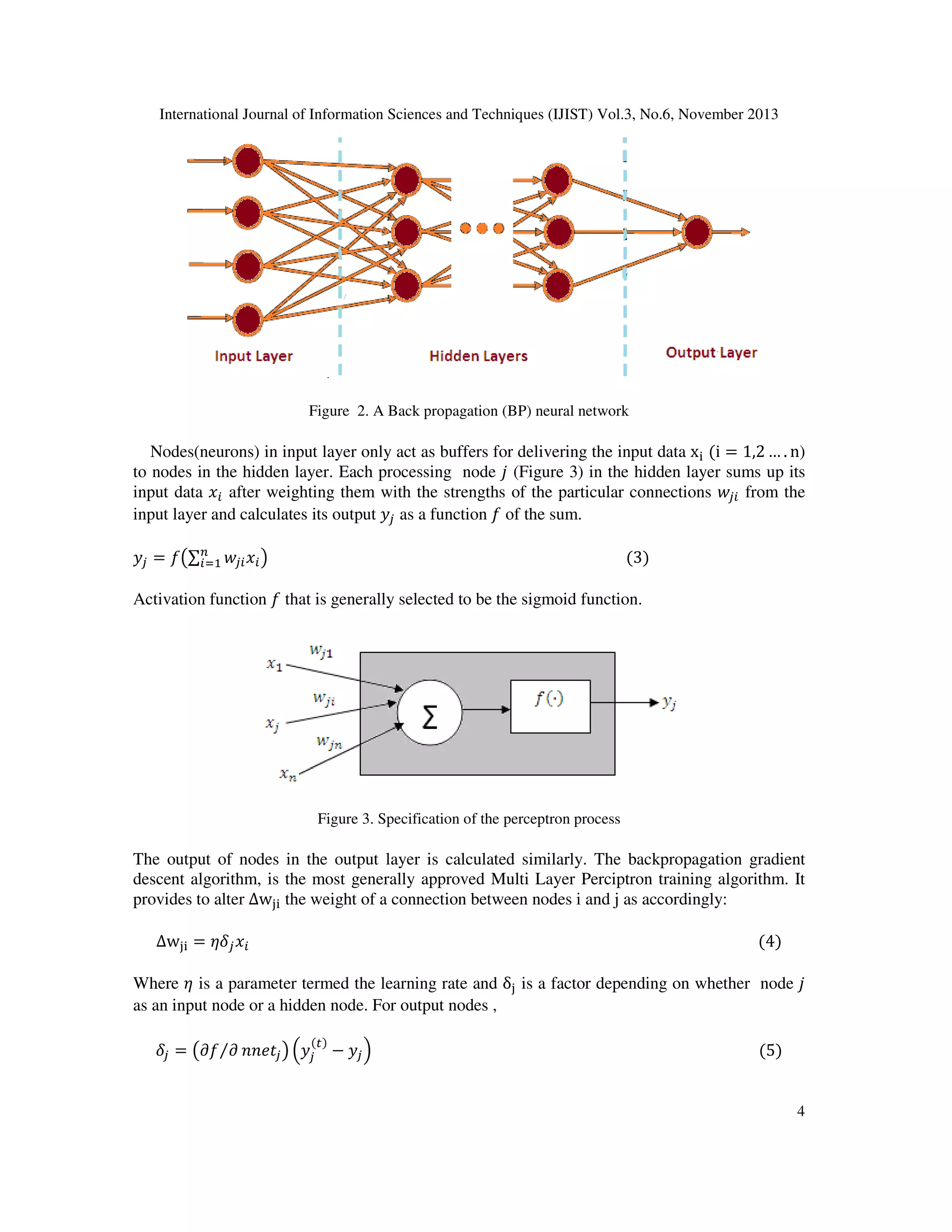
2.2 Single hidden layer feed forward neural network (SHLFNN)
The clearest form of neural network is one among a single input layer and an output layer of
nodes. The network in Figure 1 represents this type of neural network. Strictly, this is mentioned
to as a one-layer feed forward network among two outputs on account of the output layer is the
alone layer with an activation computation.
2](https://image.slidesharecdn.com/performanceanalysisofneuralnetworkmodelsforoxazolinesandoxazolesderivativesdescriptordataset-131207023119-phpapp02/75/Performance-analysis-of-neural-network-models-for-oxazolines-and-oxazoles-derivatives-descriptor-dataset-2-2048.jpg)
![International Journal of Information Sciences and Techniques (IJIST) Vol.3, No.6, November 2013
and for hidden nodes
ߜ = ൫߲݂⁄߲ ݊݊݁ݐ ൯ ቌ ݓ ߜ ቍ ሺ6ሻ
In Eq. (5) , ݊݊݁ݐ is the aggregate weighted sum of input data to nodes ݆ and ݕ is the target
output for node ݆. As there are no target outputs for hidden nodes ,in Eq. (6) , the variation
between the target and measured output of a hidden nodes ݆ is put back by the weighted aggregate
of the ߜ terms at present obtained for nodes ݍlinked to the output of node ݆ The method starts
with the output layer , the ߜ term is calculated for nodes in entire layers and weight updates
detected for all links, repetitively. The weight updating method can happen after the presentation
of each training observation (observation-based training) or after the presentation of the whole set
of training observations. Training epoch is achieved when all training patterns have been
introduced once to the Multilayer Perceptron.
ሺ௧ሻ
2.4 Gradient Descent Back Propagation with Momentum Neural Network
(GDBPMNN)
Gradient descent back propagation with momentum neural network (GDBPMNN) algorithm is
widely used in neural network training, and its convergence is discussed. A momentum term is
often added to the GDBPNN algorithm in order to accelerate and stabilize the learning procedure
in which the present weight updating increment is a mixture of the current gradient of the error
function and the prior weight revising increment. Gradient decent back propagation with
momentum allows a neural network to respond not only to the local gradient, but also to recent
tendency in the error surface. Momentum allows the neural network to ignore small features in
the error surface. Without momentum a neural network may get stranded in a shallow local
minimum. With momentum a network can move through such a least.
Momentum can be combined to GDBPNN method learning by building weight alters balance to
the sum of a portion of the final weight modification and the new modification advised by the
GDBP rule. The importance of the response that the last weight modification is admitted to have
is negotiated by a momentum constant, ߤ , which can be any number between 0 and 1. When the
momentum constant is 0 a weight modification is based only on the gradient. When the
momentum constant is 1 the new weight modification is set to balance the last weight
modification and the gradient is plainly neglected.
∆ݓ ሺ1 + ܫሻ = ߟߜ ݔ + ߤ∆ݓ ሺܫሻ ሺ7ሻ
where ∆ݓ ሺ1 + ܫሻ and ∆ݓ ሺܫሻ are weight alters in epochs ሺ1 + ܫሻand ሺܫሻ, suitable way[24].
2.5 Back propagation with Weight Decay Neural Network (BPWDNN)
Back propagation of error gradients for back propagation neural networks has proven to be useful
in layered feed forward neural network training. Still, a wide number of repetitions is commonly
required for changing the weights. The problem becomes more critical especially when a high
level of accuracy is required. The complexity of a back propagation neural network can be
regulated by a hyper-parameter called “weight decay” to penalize the weights of hidden nodes.
5](https://image.slidesharecdn.com/performanceanalysisofneuralnetworkmodelsforoxazolinesandoxazolesderivativesdescriptordataset-131207023119-phpapp02/75/Performance-analysis-of-neural-network-models-for-oxazolines-and-oxazoles-derivatives-descriptor-dataset-5-2048.jpg)
![International Journal of Information Sciences and Techniques (IJIST) Vol.3, No.6, November 2013
ݓ ሺI + 1ሻ = −ߣ ቆ
∂E୧
2λη
ሺIሻ ۊሺ13ሻ
ቇ ሺIሻ + − 1ۇ
ଶ ݓ
∂ݓ
ଶ ሺIሻቁ
ቀ1 + w୧୨
ۉ
ی
It can be demonstrates that in this case small weights decrease more swiftly than large ones.
2.6 Quantile Regression Neural Network (QRNN)
Artificial neural networks allow the estimation of in some way nonlinear models without the need
to define a accurate functional form. The most widely-used neural network for predicting is the
single hidden layer feed forward neural network [25]. It exists a set of n input nodes , which are
connected to each of m nodes in a single hidden layer, which, in turn, are connected to an output
node. The final model can be made as
݂ሺݔ௧ , ݓ ,ݒሻ = ݃ଶ ൮ ݒ ݃ଵ ൭ ݓ ݔ௧ ൱൲ ሺ14ሻ
ୀ
ୀ
where gଵ ሺ·ሻ and g ଶ ሺ·ሻ are activation functions, which are commonly chosen as sigmoidal and
linear accordingly , w୨୧ and v୨ are the weights to be approximated.
Theoretical assist for the use of quantile regression within an artificial neural network for the
evaluation of probably nonlinear quantile models [26]. The only other work that we are
knowledgeable of, that considers quantile regression neural networks , is that of Burgess [27] who
briefly explains the proposal of the method. Alternative way of linear quantile function using the
equation in (14) , a quantile regression neural network model, ݂ሺݔ௧ , ݓ ,ݒሻ,of the ߠݐℎ quantile can
be estimated using the following minimisation.
min ቌ
௩,௪
௧|௬ ஹሺ௫ ,௩,௪ሻ
ߠ|ݕ௧ − ݂ሺݔ௧ , ݓ ,ݒሻ| +
+
ߣଶ ݒଶ ቇ ሺ15ሻ
௧|௬ ஹሺ௫ ,௩,௪ሻ
ଶ
ሺ1 − ߠሻ|ݕ௧ − ݂ሺݔ௧ , ݓ ,ݒሻ| + ߣଵ ݓ
,
where λଵ and λଶ are regularisation parameters which penalise the complicatedness of the neural
network and thus prevent over fitting [28].
2.7 Fitting and comparing models
The solutions for the SHLFFNN , GDBPNN, GDBPMNN, BPWDNN and QRNN models were
computed using open source CRAN R packages nnet ,neuralnet, RSSNS and qrnn. These five
neural network models are trained on a Oxazolines and Oxazoles derivatives descriptor dataset ,
it constructs a predictive model that returns a minimization in error when the neural network's
prediction (its output) is compared with a known or expected outcome. The comparison between
the five models were assessed using root mean square error (RMSE) and coefficient of
7](https://image.slidesharecdn.com/performanceanalysisofneuralnetworkmodelsforoxazolinesandoxazolesderivativesdescriptordataset-131207023119-phpapp02/75/Performance-analysis-of-neural-network-models-for-oxazolines-and-oxazoles-derivatives-descriptor-dataset-7-2048.jpg)
![determination Rଶ . RMSE presents information on the short term efficiency which is a benchmark
of the difference of predicated values about the observed values. The lower the RMSE, the more
accurate is the evaluation and coefficient of determination (also called R square) measures the
variance that is interpreted by the model, which is the reduction of variance when using the
model. ܴ ଶ orders from 0 to 1 while the model has healthy predictive ability when it is near to 1
and is not analyzing whatever when it is near to 0. These performance metrics are a good
measures of the overall predictive accuracy.
International Journal of Information Sciences and Techniques (IJIST) Vol.3, No.6, November 2013
MAE(mean absolute error) is an indication of the average deviation of the predicted values from
the corresponding observed values and can present information on long term performance of the
models; the lower MAE the better is the long term model prediction. Relative squared error
(RSE) is the aggregate squared error produce relative to what the error would have been if the
prediction had been the average of the absolute value. Lower RSE is the better model prediction.
The Mean Percent Error (MPE) is a well known measure that corrects the 'cancelling out' results
and also keeps into basis the different scales at which this measure can be calculated and thus can
be used to analyze different predictions. The expressions of all measures are given below.
1
= ܧܣܯ|ݕ − ݕ | ሺ16ሻ
ො
݊
ୀଵ
1
ݕ − ݕ
ො
= ܧܲܯ
∗ 100 ሺ17ሻ
݊
ݕ
ܴܵ= ܧ
ୀଵ
∑ ሺݕ − ݕ ሻଶ
ୀଵ ො
ሺ18ሻ
ሺ݉݁ܽ݊ሺݕሻ
∑ୀଵ
− ݕ ሻଶ
where ݕ and ݕ are observed and predicted values.
ො
2.9 Benchmark Experiments
Move in benchmark experiments for comparison of neural network models. The experimental
performance distributions of a set of neural network models are estimated, compared, and
ordered. The resampling process used in these experiments must be investigate in further detail to
determine which method produces the most accurate analysis of model influence. Resampling
methods to be compared include cross-validation [29-31]. We can use resampling results to make
orderly and in orderly comparisons between models [29-30]
Each model performs 25
independent runs on each sub sample and report minimum, median, maximum, mean of each
performance measure over the 25 runs.
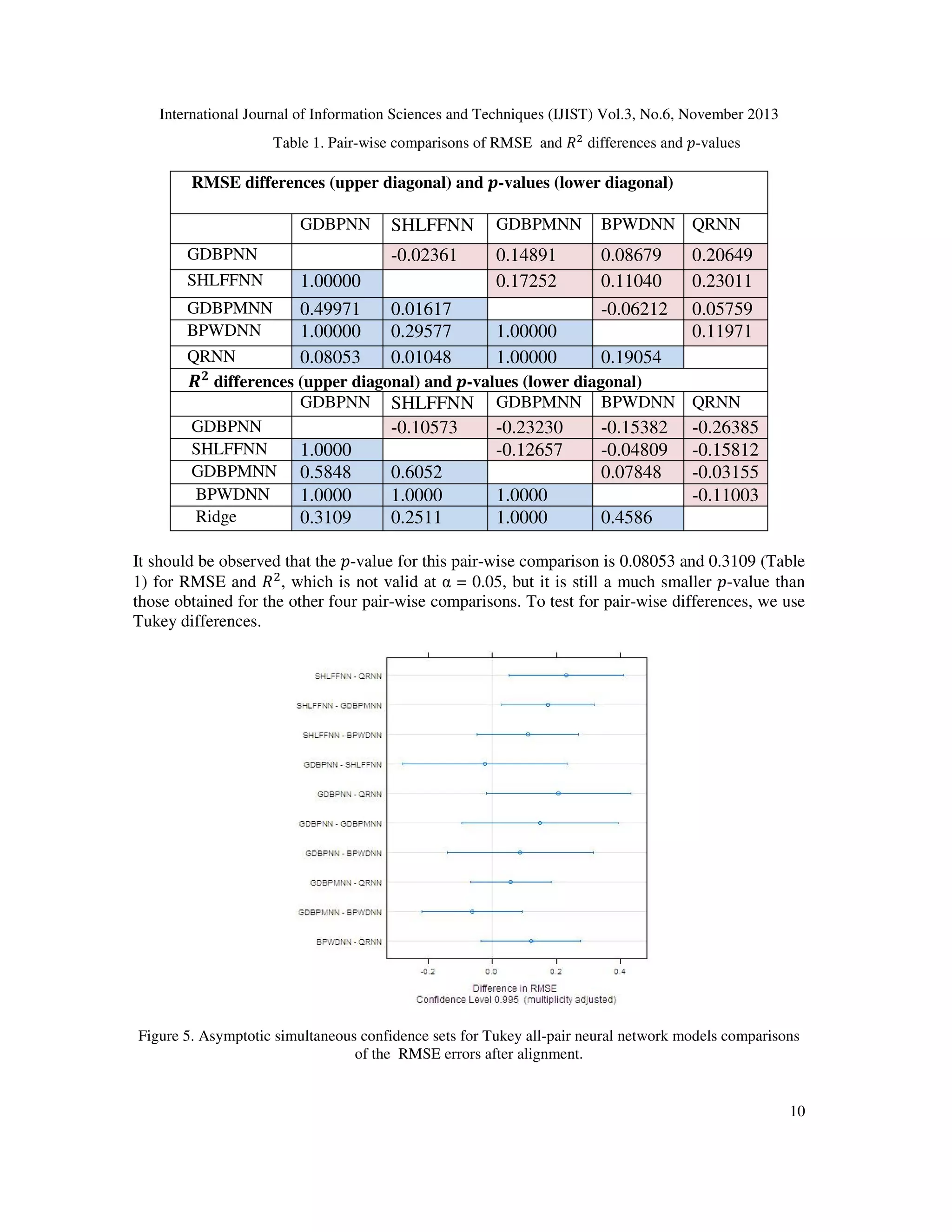
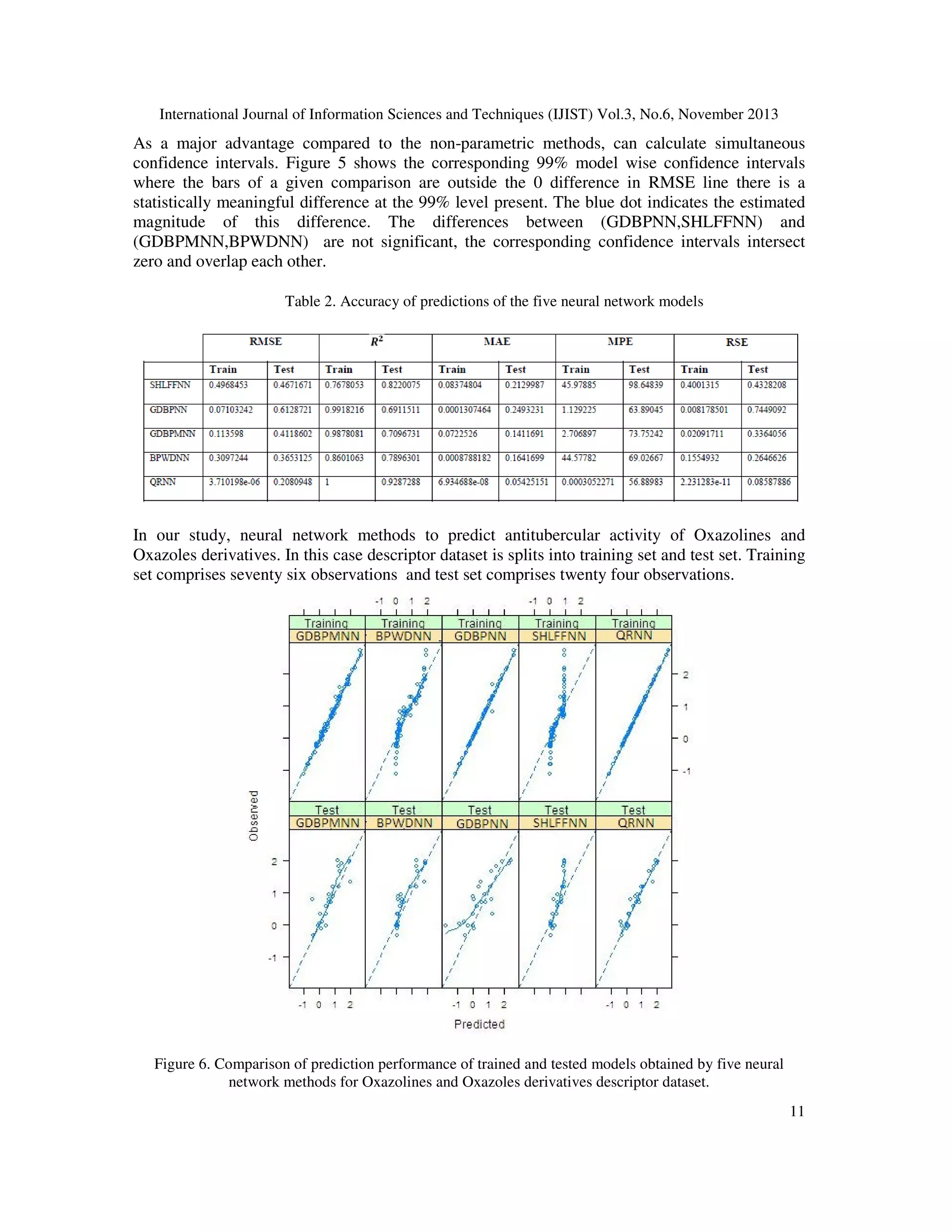
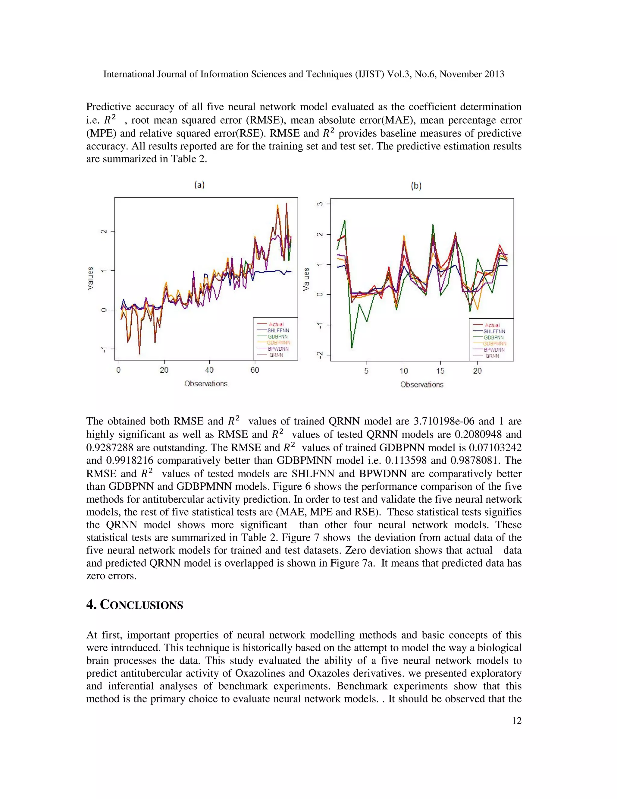
3. RESULTS AND DISCUSSION
This part presents the numerical analysis conducted using numerous neural network methods.
RMSE and ܴ ଶ values were used to analyze model prediction accuracies for the
SHLFFNN,GDBPNN, GDBPMNN, BPWDNN and QRNN neural network models. Comparing
the resampling performance the effect of prediction of antituberculer activity using Oxazolines
and Oxazoles derivatives are demonstrated in Figure 4.
8](https://image.slidesharecdn.com/performanceanalysisofneuralnetworkmodelsforoxazolinesandoxazolesderivativesdescriptordataset-131207023119-phpapp02/75/Performance-analysis-of-neural-network-models-for-oxazolines-and-oxazoles-derivatives-descriptor-dataset-8-2048.jpg)
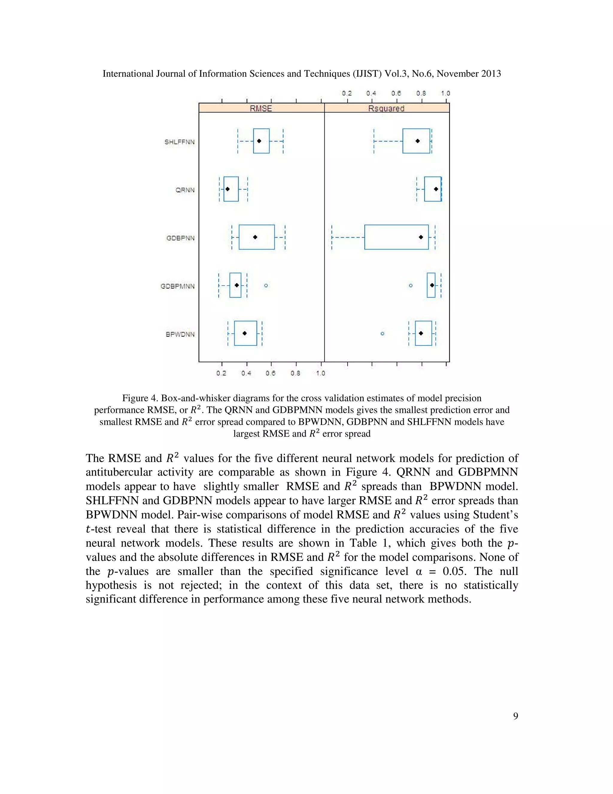
![International Journal of Information Sciences and Techniques (IJIST) Vol.3, No.6, November 2013
scheme can be utilized to compare a set of neural network techniques but does not offer a neural
network model selection. The results for the non linear neural network models suggest that we
may detect performance differences with fairly high power. We have compared the predictive
accuracies with all five neural network models among QRNN model is outperformed overall
predictive performance.
ACKNOLDGEMENTS
We thankful to the Department of Computer Science Mangalore University, Mangalore India for
technical support of this research.
REFERENCES
[1]
[2]
[3]
[4]
[5]
[6]
[7]
[8]
[9]
[10]
[11]
[12]
[13]
[14]
[15]
[16]
Kesavan, J.G., Peck, G.E., 1996.,”Pharmaceutical granulation and tablet formulation using neural
networks.”,Pharm. Dev. Technol. 1, 391–404.
Takahara, J., Takayama, K., Nagai, T., 1997. ,“Multi-objective simultaneous optimization technique
based on an artificial neural network in sustained release formulations.”, J. Control. Release 49, 11–
20.
Takayama, K., Fujikawa, M., Nagai, T., 1999. ,“Artificial neural networks as a novel method to
optimize pharmaceutical formulations. “, Pharm. Res. 16, 1–6.
Chen, Y., McCall, T.W., Baichwal, A.R., Meyer, M.C., 1999. ,”The application of an artificial neural
network and
pharmacokinetic simulations in the design of controlled-release dosage forms. J.
Control. Release 59, 33–41.
Wu, T., Pan,W., Chen, J., Zhang, R., 2000. ,“Formulation optimization technique based on artificial
neural network in salbutamol sulfate osmotic pump tablets.”, Drug Dev. Ind. Pharm. 26, 211–215.
Bourquin, J., Schmidli, H., Hoogevest, P.V., Leuenberger, H., 1997b. ,“Basic concepts of artificial
neural networks (ANN) modeling in the application to pharmaceutical development. “,Pharm. Dev.
Tech. 2, 95–109.
Achanta, A.S., Kowalski, J.G., Rhodes, C.T., 1995. ,"Artificial neural networks: implications for
pharmaceutical sciences.", Drug Dev. Ind. Pharm. 21, 119–155
Cheng F, Vijaykumar S (2012) ,“Applications of Artificial Neural Network Modelling in Drug
Discovery. “, Clin Exp Pharmacol 2:e113. doi: 10.4172/2161-1459.1000e113
ALI AKCAYOL, M. and CINAR, Can.(20050 ,“Artificial neural network based modelling of heated
catalytic converter performance.”, Applied Thermal Engineering , vol. 25, no. 14-15, p. 2341-2350.
KOSE, Erdogan.(2008), “Modelling of colour perception of different age groups using artificial
neural networks.”, Expert Systems with Applications, vol. 34, no.3, p. 2129-2139.
C. ZOU and L. ZHOU,“QSAR study of oxazolidinone antibacterial agents using artificial neural
networks”, Molecular Simulation, Vol. 33, No. 6, –530
LiHong Hu , GuanHua Chen , Raymond Ming-Wah Chau (2006),“A neural networks-based drug
discovery approach and its application for designing aldose reductase inhibitors”, Journal of
Molecular Graphics and Modelling 24 244–253
Huang GB, Chen YQ, Babri HA (2000),”Classification ability of single hidden layer feedforward
neural networks”, IEEE Trans Neural Netw. ;11(3):799-801. doi: 10.1109/72.846750.
Udo Seiffert and Bernd Michaelis (2000),“On the Gradient Descent in BackPropagation and its
substitution by a genetic algorithm”, Proceedings of the IASTED International Conference Applied
Informatics
Ning Qian (1999) ,“On the momentum term in gradient descent learning algorithms”, Neural
Networks 12 145-151
M. Z. Rehman, N. M. Nawi (2011),“ Improving the Accuracy of Gradient Descent Back Propagation
Algorithm (GDAM) on Classification Problems”, International Journal on New Computer
Architectures and Their Applications ISSN: 2220-9085)1(4): 838-847
13](https://image.slidesharecdn.com/performanceanalysisofneuralnetworkmodelsforoxazolinesandoxazolesderivativesdescriptordataset-131207023119-phpapp02/75/Performance-analysis-of-neural-network-models-for-oxazolines-and-oxazoles-derivatives-descriptor-dataset-13-2048.jpg)
![International Journal of Information Sciences and Techniques (IJIST) Vol.3, No.6, November 2013
[17] Amit Gupta, Siuwa M. Lam (1998) ,“Weight decay backpropagation for noisy data”, Neural
Networks Pages 1127–1138
[18] Taylor, J.W., (2000).,” A quantile regression neural network approach to estimating the conditional
density of multiperiod returns.”, Journal of Forecasting, 19(4): 299-311.
[19] Andrew J. Phillips, Yoshikazu Uto, Peter Wipf, Michael J. Reno, and David R. Williams, (2000)
“Synthesis of Functionalized Oxazolines and Oxazoles with DAST and Deoxo-Fluor” Organic Letters
Vol 2 ,No.8 1165-1168
[20] Moraski GC, Chang M, Villegas-Estrada A, Franzblau SG, Möllmann U, Miller
MJ(2010).,”Structure-activity relationship of new anti-tuberculosis agents derived from oxazoline and
oxazole benzyl esters” ,Eur J Med Chem. 45(5):1703-16. doi: 10.1016/j.ejmech.2009.12.074. Epub
2010 Jan 14.
[21] Yap CW* (2011). PaDEL-Descriptor: An open source software to calculate molecular descriptors and
fingerprints. Journal of Computational Chemistry. 32 (7): 1466-1474.
[23] Smits, J. R. M., Melssen, W. J., Buydens, L. M. C., & Kateman, G. (1994). ,”Using artificial neural
networks for solving chemical problems. Part I. Multi-layer feed-forward networks. “,Chemom.
Intell. Lab., 22, 165-189.
[24] D.E. Rumelhart, G.E. Hinton, and R.J. Williams (1986), “Learning representations by backpropagating Errors”, Nature, 323 , 533-536.
[25] Zhang, G., Patuwo, B.E. and Hu, M.Y.(1998), "Forecasting with Artificial Neural Networks: The
State of the Art", International Journal of Forecasting, 14 , 35-62.
[26] White, H.A.R. Gallant et al.(1992),"Nonparametric Estimation of Conditional Quantiles Using Neural
Networks", Artificial Neural Networks: Approximation and Learning Theory, Cambridge and Oxford,
Blackwell , 191-205.
[27] Burgess, A.N.(1995), ‘Robust Financial Modelling by Combining Neural Network Estimators of
Mean and Median’, Proceedings of Applied Decision Technologies, UNICOM Seminars, Brunel
University, London, UK.
[28] Bishop, C.M.(1997), “Neural Networks for Pattern Recognition”, Oxford, Oxford University Press.
[29] Hothorn et al(2005)., “The design and analysis of benchmark experiments.”, Journal of
Computational and Graphical Statistics vol. 14 (3) pp. 675-699
[30] Olaf Mersmann, Heike Trautmann1, Boris Naujoks and Claus Weihs (2010), “Benchmarking
Evolutionary
Multiobjective
Optimization
Algorithms”,
http://www.statistik.tudortmund.de/fileadmin/user_uploaddortmund.de/fileadmin/user_upload/SFB_823/
discussion_papers/2010/DP_0310_SFB823_Mersmann_Trautmann_etal.pdf
[31] Eugster M. J. A. et al., (2008), “Exploratory and Inferential Analysis of Benchmark Experiments.”,
Technical Report Number 030, Dept. of Statistics, University of Munich.
14](https://image.slidesharecdn.com/performanceanalysisofneuralnetworkmodelsforoxazolinesandoxazolesderivativesdescriptordataset-131207023119-phpapp02/75/Performance-analysis-of-neural-network-models-for-oxazolines-and-oxazoles-derivatives-descriptor-dataset-14-2048.jpg)


This paper evaluates the performance of five distinct neural network models in predicting the antitubercular activity of oxazolines and oxazoles derivatives. The models include single hidden layer feed forward neural network (SHLFNN), gradient descent back propagation neural network (GDBPNN), gradient descent back propagation with momentum neural network (GDBPMNN), back propagation with weight decay neural network (BPWDNN), and quantile regression neural network (QRNN), with QRNN demonstrating superior predictive accuracy. The study illustrates how neural networks can effectively model non-linear molecular descriptor data for drug discovery.


![Vibe Coding vs. Spec-Driven Development [Free Meetup]](https://cdn.slidesharecdn.com/ss_thumbnails/vibecodingvsspecdrivendevelopment-251209105622-43f455e7-thumbnail.jpg?width=640&height=640&fit=bounds)