This document provides an overview of pattern recognition and machine learning concepts. It discusses features and feature vectors, patterns and classifiers. It describes the components of a typical pattern recognition system including sensors, preprocessing, feature extraction, and classification algorithms. It then provides an example of using a vision system and robotic arm to sort fish by species. It analyzes features, builds classifiers, and discusses improving classification accuracy. Finally, it reviews key probability and statistics concepts used in pattern recognition like Bayes' theorem, probability distributions, expectation, variance and covariance.


![Intelligent Sensor Systems
Ricardo Gutierrez-Osuna
Wright State University
11
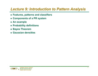
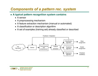
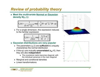
Review of probability theory
g Probability
n Probabilities are numbers assigned to events that indicate “how likely” it
is that the event will occur when a random experiment is performed
g Conditional Probability
n If A and B are two events, the probability of event A when we already
know that event B has occurred P[A|B] is defined by the relation
g P[A|B] is read as the “conditional probability of A conditioned on B”,
or simply the “probability of A given B”
A1
A2
A3
A4
event
probability
A1 A2 A3
Probability
Law
A4
Sample space
0
P[B]
for
P[B]
B]
P[A
B]
|
P[A >
=
I](https://image.slidesharecdn.com/pattern-analysis1-230403003236-c034215c/85/Pattern-Analysis-1-pdf-11-320.jpg)
![Intelligent Sensor Systems
Ricardo Gutierrez-Osuna
Wright State University
12
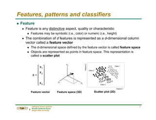
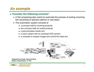
Review of probability theory
g Conditional probability: graphical interpretation
g Theorem of Total Probability
n Let B1, B2, …, BN be mutually exclusive events, then
S S
“B has
occurred”
A A∩B B A A∩B B
∑
=
=
+
=
N
1
k
k
k
N
N
1
1 ]
]P[B
B
|
P[A
]
]P[B
B
|
...P[A
]
]P[B
B
|
P[A
P[A]
B1
B2
B3
BN-1
BN
A](https://image.slidesharecdn.com/pattern-analysis1-230403003236-c034215c/85/Pattern-Analysis-1-pdf-12-320.jpg)
![Intelligent Sensor Systems
Ricardo Gutierrez-Osuna
Wright State University
13
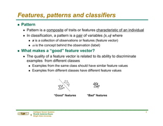
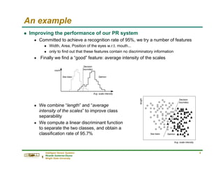
Review of probability theory
g Bayes Theorem
n Given B1, B2, …, BN, a partition of the sample space S. Suppose that
event A occurs; what is the probability of event Bj?
n Using the definition of conditional probability and the Theorem of total
probability we obtain
n Bayes Theorem is definitely the
fundamental relationship in
Statistical Pattern Recognition
∑
=
⋅
⋅
=
= N
1
k
k
k
j
j
j
j
]
P[B
]
B
|
P[A
]
P[B
]
B
|
P[A
P[A]
]
B
P[A
A]
|
P[B
I
Rev. Thomas Bayes (1702-1761)](https://image.slidesharecdn.com/pattern-analysis1-230403003236-c034215c/85/Pattern-Analysis-1-pdf-13-320.jpg)

![Intelligent Sensor Systems
Ricardo Gutierrez-Osuna
Wright State University
16
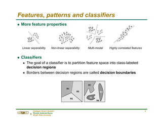
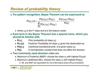
Review of probability theory
g The covariance matrix (cont.)
n The covariance terms can be expressed as
g where ρik is called the correlation coefficient
g Graphical interpretation
=
−
−
−
−
−
−
−
−
=
−
−
=
∑
=
2
N
1N
1N
2
1
N
N
N
N
1
1
N
N
N
N
1
1
1
1
1
1
T
...
c
...
...
c
...
)]
)(x
E[(x
...
)]
)(x
E[(x
...
)]
)(x
E[(x
...
)]
)(x
E[(x
]
;
E[(X
COV[X]
σ
σ
O
Xi
Xk
Cik=-σiσk
ρik=-1
Xi
Xk
Cik=-½σiσk
ρik=-½
Xi
Xk
Cik=0
ρik=0
Xi
Xk
Cik=+½σiσk
ρik=+½
Xi
Xk
Cik=σiσk
ρik=+1
k
i
ik
ik
2
i
ii c
and
c σ
σ
ρ
σ =
=](https://image.slidesharecdn.com/pattern-analysis1-230403003236-c034215c/85/Pattern-Analysis-1-pdf-16-320.jpg)


![[ppt]](https://cdn.slidesharecdn.com/ss_thumbnails/ppt2931-thumbnail.jpg?width=640&height=640&fit=bounds)
![[ppt]](https://cdn.slidesharecdn.com/ss_thumbnails/ppt3441-thumbnail.jpg?width=640&height=640&fit=bounds)


