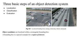
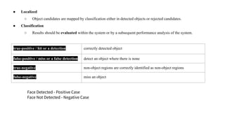
Localization, Classification, and
Evaluation
Agenda
● Introduction
● Descriptors, Classifiers, and Learning
● Performance of Object Detectors
Three basic steps of an object detection system
● Localization
● Classification
● Evaluation
Object candidates are localized within a rectangular bounding box.
A bounding box is a special example for a region of interest.
● Localized
○ Object candidates are mapped by classification either in detected objects or rejected candidates.
● Classification
○ Results should be evaluated within the system or by a subsequent performance analysis of the system.
true-positive / hit or a detection correctly detected object
false-positive / miss or a false detection detect an object where there is none
true-negative non-object regions are correctly identified as non-object regions
false-negative miss an object
Face Detected - Positive Case
Face Not Detected - Negative Case
● One false-positive (the largest square)
● Two false-negatives (a man in the middle and a girl on the right of the image).
● A head seen from the side (one case in the figure) does not define a face.
Descriptors, Classifiers, and Learning
● Classification is defined by membership in constructed pairwise-disjoint classes being
subsets of Rn
for a given value n > 0.
● In other words, classes define a partitioning of the space Rn
.
● Time-efficiency is an important issue when performing classification.
● This subsection only provides a few brief basic explanations for the extensive area of
classification algorithms.
Descriptors
● A descriptor x = (x1
, . . . , xn
) is a point in an n-dimensional real space Rn
, called
descriptor space.
● A descriptor also called a feature.
● A feature in an image that, as commonly used in image analysis, combines a keypoint and
a descriptor.
● Thus, we continue to use “descriptor” rather than “feature” for avoiding confusion.
● It representing measured or calculated property values in a given order an illustration for
n = 2 (Eg: a SIFT descriptor is of length n = 128).
● Example: A descriptor x1
= (621.605, 10940) for Segment 1 in this descriptor space
defined by the properties “perimeter” and “area”.
Classifiers
● A classifier assigns class numbers to descriptors, typically, first, to a given set {x1
,
. . . , xm
} of already-classified descriptors for training (the learning set), and then to
the descriptors generated for recorded image/video data while being applied:
○ A (general) classifier assigns class numbers 1, 2, . . . , k for k > 1 classes and 0
for ‘not classified’.
○ A binary classifier assigns class numbers −1 and +1 in the cases where we are
only interested whether a particular event (Eg: ‘driver has closed eyes’) occurs,
specified by output +1.
● A classifier is weak if it does not perform up to expectations (Eg: it might be just a
bit better than random guessing).
● Multiple weak classifiers can be mapped into a strong classifier, aiming at a
satisfactory solution of a classification problem.
● A statistical combination of multiple weak classifiers into one strong classifier.
● Weak or strong classifiers can be general-case (i.e. multi-class)
● classifiers or just binary classifiers; just being “binary” does not define “weak”.
Example 10.1 (Binary Classifier by Linear Separation
● A binary classifier may be defined by constructing a hyperplane Π : wT
x + b = 0
in Rn
for n ≥ 1.
● Vector w ∈ Rn
is the weight vector, and the real b ∈ R is the bias of Π.
● For n = 2 or n = 3, w is the gradient or normal orthogonal to the defined line or
plane, respectively.
● One side of the hyperplane (including the plane itself) defines
the value “+1”, and the other side (not including the plane
itself) the value “−1”.
● Example for n = 2; the hyperplane is a straight line in this
case, and for n = 1, it is just a point separating R1
.
h(x) = wT
x + b
● The cases h(x) > 0 or h(x) < 0 then define the class values
“+1” or “−1” for one side of the hyperplane Π.
● Such a linear classifier (i.e. defined by the weight vector w and bias b) can be calculated
for a distribution of (pre-classified) training descriptors in the n D descriptor space if the
given distribution is linear separable.
● If this is not the case, then we define the error for a misclassified descriptor x by its
perpendicular distance to the hyperplane Π.
d2
(x, Π) = |wT
x + b| / ǁwǁ2
● The task is to calculate a hyperplane Π such that the total error for all misclassified
training descriptors is minimized.
● This is the error defined in margin-based classifiers such as support vector machines and
is (usually) not explicitly used in AdaBoost.
Example 10.2 (Classification by Using a Binary Decision Tree)
● A classifier can also be defined by binary decisions at split nodes in a tree (i.e. “yes” or “no”).
● Each decision is formalized by a rule, and given input data can be tested whether they satisfy the rule
or not.
● Accordingly, we proceed with the identified successor node in the tree.
● Each leaf node of the tree defines finally an assignment of data arriving at this node into classes.
Example: Each leaf node can identify exactly one class in Rn
.
● The tested rules in the shown tree define straight lines in the 2D descriptor space.
● Descriptors arriving at one of the leaf nodes are then in one of the shown subsets of R2
.
● A single decision tree, or just one split node in such a tree, can be considered to be an example for a
weak classifier; a set of decision trees (called a forest) is needed for being able to define a strong
classifier.
Learning
● Learning is the process of defining or training a classifier based on a
set of descriptors; classification is then the actual application of the
classifier.
● During classification, we may also identify some mis-behaviour (e.g.
“assumed” mis-classifications), and this again can lead to another
phase of learning.
● The set of descriptors used for learning may be pre-classified or not.
Supervised Learning
● In supervised learning we assign class numbers to descriptors
“manually” based on expertise.
Example: “Yes, the driver does have closed eyes in this image”.
● As a result, we can define a classifier by locating optimized separating
manifolds in Rn
for the training set of descriptors.
● A hyperplane Π is the simplest case of an optimized separating
manifold.
● An alternative use of expert knowledge for supervised learning is the
specification of rules at nodes in a decision tree.
● This requires knowledge about possible sequences of decisions.
Unsupervised Learning
● In unsupervised learning we do not have prior knowledge about class memberships
of descriptors.
● When aiming at separations in the descriptor space, we may apply a clustering
algorithm for a given set of descriptors for identifying a separation of Rn
into
classes.
● Example: We may analyse the density of the distribution of given descriptors in Rn
;
● A region having a dense distribution defines a seed point of one class, and then we
assign all descriptors to identified seed points by applying, for example, the
nearest-neighbour rule.
● When aiming at defining decision trees for partitioning the descriptor space, we can
learn decisions at nodes of a decision tree based on some general data analysis
rules.
● The data distribution then “decides” about the generated rules.
Combined Learning Approaches
● There are also cases where we may combine supervised learning with
strategies known from unsupervised learning.
● Example: We can decide whether a given image window, also called
a bounding box, shows a pedestrian.
● This defines the supervised part in learning.
● We can also decide for a patch, being a subwindow of a bounding
box, whether it possibly belongs to a pedestrian.
● Example: The head of the cyclist is also considered to belong
possibly to a pedestrian.
● When we generate descriptors for bounding boxes or patches (e.g.
measured image intensities at selected pixel locations),
● Then we cannot decide anymore manually for each individual
descriptor whether it is characteristic for a pedestrian or not.
● Example: for a set of given image windows, we know that they are
all parts of pedestrians, and the algorithm designed for generating a
classifier decides at some point to use a particular feature of those
windows for processing them further.
● This particular feature might not be generic in the sense that it
separates any window showing a part of a pedestrian from any
window showing no part of a pedestrian.
● Such an “internal” mechanism in a program that generates a classifier
defines an unsupervised part in learning.
● The overall task is to combine available supervision with
unsupervised data analysis when generating a classifier.
Performance of Object Detectors
● Object Detector → Applying a classifier for an object detection problem.
● Evaluations of designed object detectors are required to compare their performance under particular conditions.
● There are common measures in pattern recognition or information retrieval for performance evaluation of
classifiers.
● TP = 12, FP = 1, and FN = 2, TN = None
● In this figure doesn’t indicate how many
non-object regions have been analysed and
correctly identified as being no faces.
● We can’t specify the number TN.
● We need to analyse the applied classifier for
obtaining TN.
● Thus, TN is not a common entry for performance
measures.
Precision (PR) Recall (RC)
It is the ratio of true-positives compared to all
detections.
Itis the ratio of true-positives compared to all potentially
possible detections
PR = 1, termed 1-precision, means that no
false-positive is detected.
RC = 1 means that all the visible objects in an image are
detected and that there is no false-negative.
TP = 1
FP = 2
PR = 1/(1+2)
= 1/3
Convert to 100% = (1/3) x 100
= 33%
Miss Rate (MR) False-Positives per Image (FPPI)
It is the ratio of false-negatives compared to all objects
in an image.
It is the ratio of false-positives compared to all detected
objects.
MR = 0 means that all the visible objects in the image
are detected, which is equivalent to RC = 1.
FPPI = 0 means that all the detected objects are correctly
classified, which is equivalent to 1-precision.
MR = 0 means that all the visible objects in the image
are detected, which is equivalent to RC = 1.
FPPI = 0 means that all the detected objects are correctly
classified, which is equivalent to 1-precision.
True-Negative Rate (TNR) Accuracy (AC)
It is the ratio of true-negatives com-
pared to all decisions in “no-object” regions.
It is the ratio of false-positives compared to all detected
objects.
MR = 0 means that all the visible objects in the image
are detected, which is equivalent to RC = 1.
The accuracy is the ratio of correct decisions compared to all
decisions.
We are usually not interested in numbers of true-negatives, these two measures have less significance in performance
evaluation studies.
Localization, Classification, and Evaluation.pdf

Localization, Classification, and Evaluation.pdf

  • 1.
  • 2.
    Agenda ● Introduction ● Descriptors,Classifiers, and Learning ● Performance of Object Detectors
  • 3.
    Three basic stepsof an object detection system ● Localization ● Classification ● Evaluation Object candidates are localized within a rectangular bounding box. A bounding box is a special example for a region of interest.
  • 4.
    ● Localized ○ Objectcandidates are mapped by classification either in detected objects or rejected candidates. ● Classification ○ Results should be evaluated within the system or by a subsequent performance analysis of the system. true-positive / hit or a detection correctly detected object false-positive / miss or a false detection detect an object where there is none true-negative non-object regions are correctly identified as non-object regions false-negative miss an object Face Detected - Positive Case Face Not Detected - Negative Case
  • 6.
    ● One false-positive(the largest square) ● Two false-negatives (a man in the middle and a girl on the right of the image). ● A head seen from the side (one case in the figure) does not define a face.
  • 7.
    Descriptors, Classifiers, andLearning ● Classification is defined by membership in constructed pairwise-disjoint classes being subsets of Rn for a given value n > 0. ● In other words, classes define a partitioning of the space Rn . ● Time-efficiency is an important issue when performing classification. ● This subsection only provides a few brief basic explanations for the extensive area of classification algorithms.
  • 8.
    Descriptors ● A descriptorx = (x1 , . . . , xn ) is a point in an n-dimensional real space Rn , called descriptor space. ● A descriptor also called a feature. ● A feature in an image that, as commonly used in image analysis, combines a keypoint and a descriptor. ● Thus, we continue to use “descriptor” rather than “feature” for avoiding confusion. ● It representing measured or calculated property values in a given order an illustration for n = 2 (Eg: a SIFT descriptor is of length n = 128). ● Example: A descriptor x1 = (621.605, 10940) for Segment 1 in this descriptor space defined by the properties “perimeter” and “area”.
  • 10.
    Classifiers ● A classifierassigns class numbers to descriptors, typically, first, to a given set {x1 , . . . , xm } of already-classified descriptors for training (the learning set), and then to the descriptors generated for recorded image/video data while being applied: ○ A (general) classifier assigns class numbers 1, 2, . . . , k for k > 1 classes and 0 for ‘not classified’. ○ A binary classifier assigns class numbers −1 and +1 in the cases where we are only interested whether a particular event (Eg: ‘driver has closed eyes’) occurs, specified by output +1.
  • 11.
    ● A classifieris weak if it does not perform up to expectations (Eg: it might be just a bit better than random guessing). ● Multiple weak classifiers can be mapped into a strong classifier, aiming at a satisfactory solution of a classification problem. ● A statistical combination of multiple weak classifiers into one strong classifier. ● Weak or strong classifiers can be general-case (i.e. multi-class) ● classifiers or just binary classifiers; just being “binary” does not define “weak”.
  • 12.
    Example 10.1 (BinaryClassifier by Linear Separation ● A binary classifier may be defined by constructing a hyperplane Π : wT x + b = 0 in Rn for n ≥ 1. ● Vector w ∈ Rn is the weight vector, and the real b ∈ R is the bias of Π. ● For n = 2 or n = 3, w is the gradient or normal orthogonal to the defined line or plane, respectively.
  • 13.
    ● One sideof the hyperplane (including the plane itself) defines the value “+1”, and the other side (not including the plane itself) the value “−1”. ● Example for n = 2; the hyperplane is a straight line in this case, and for n = 1, it is just a point separating R1 . h(x) = wT x + b ● The cases h(x) > 0 or h(x) < 0 then define the class values “+1” or “−1” for one side of the hyperplane Π.
  • 15.
    ● Such alinear classifier (i.e. defined by the weight vector w and bias b) can be calculated for a distribution of (pre-classified) training descriptors in the n D descriptor space if the given distribution is linear separable. ● If this is not the case, then we define the error for a misclassified descriptor x by its perpendicular distance to the hyperplane Π. d2 (x, Π) = |wT x + b| / ǁwǁ2 ● The task is to calculate a hyperplane Π such that the total error for all misclassified training descriptors is minimized. ● This is the error defined in margin-based classifiers such as support vector machines and is (usually) not explicitly used in AdaBoost.
  • 16.
    Example 10.2 (Classificationby Using a Binary Decision Tree) ● A classifier can also be defined by binary decisions at split nodes in a tree (i.e. “yes” or “no”). ● Each decision is formalized by a rule, and given input data can be tested whether they satisfy the rule or not. ● Accordingly, we proceed with the identified successor node in the tree. ● Each leaf node of the tree defines finally an assignment of data arriving at this node into classes. Example: Each leaf node can identify exactly one class in Rn . ● The tested rules in the shown tree define straight lines in the 2D descriptor space. ● Descriptors arriving at one of the leaf nodes are then in one of the shown subsets of R2 . ● A single decision tree, or just one split node in such a tree, can be considered to be an example for a weak classifier; a set of decision trees (called a forest) is needed for being able to define a strong classifier.
  • 18.
    Learning ● Learning isthe process of defining or training a classifier based on a set of descriptors; classification is then the actual application of the classifier. ● During classification, we may also identify some mis-behaviour (e.g. “assumed” mis-classifications), and this again can lead to another phase of learning. ● The set of descriptors used for learning may be pre-classified or not.
  • 20.
    Supervised Learning ● Insupervised learning we assign class numbers to descriptors “manually” based on expertise. Example: “Yes, the driver does have closed eyes in this image”. ● As a result, we can define a classifier by locating optimized separating manifolds in Rn for the training set of descriptors. ● A hyperplane Π is the simplest case of an optimized separating manifold. ● An alternative use of expert knowledge for supervised learning is the specification of rules at nodes in a decision tree. ● This requires knowledge about possible sequences of decisions.
  • 21.
    Unsupervised Learning ● Inunsupervised learning we do not have prior knowledge about class memberships of descriptors. ● When aiming at separations in the descriptor space, we may apply a clustering algorithm for a given set of descriptors for identifying a separation of Rn into classes. ● Example: We may analyse the density of the distribution of given descriptors in Rn ; ● A region having a dense distribution defines a seed point of one class, and then we assign all descriptors to identified seed points by applying, for example, the nearest-neighbour rule. ● When aiming at defining decision trees for partitioning the descriptor space, we can learn decisions at nodes of a decision tree based on some general data analysis rules. ● The data distribution then “decides” about the generated rules.
  • 22.
    Combined Learning Approaches ●There are also cases where we may combine supervised learning with strategies known from unsupervised learning. ● Example: We can decide whether a given image window, also called a bounding box, shows a pedestrian. ● This defines the supervised part in learning. ● We can also decide for a patch, being a subwindow of a bounding box, whether it possibly belongs to a pedestrian. ● Example: The head of the cyclist is also considered to belong possibly to a pedestrian.
  • 23.
    ● When wegenerate descriptors for bounding boxes or patches (e.g. measured image intensities at selected pixel locations), ● Then we cannot decide anymore manually for each individual descriptor whether it is characteristic for a pedestrian or not. ● Example: for a set of given image windows, we know that they are all parts of pedestrians, and the algorithm designed for generating a classifier decides at some point to use a particular feature of those windows for processing them further.
  • 24.
    ● This particularfeature might not be generic in the sense that it separates any window showing a part of a pedestrian from any window showing no part of a pedestrian. ● Such an “internal” mechanism in a program that generates a classifier defines an unsupervised part in learning. ● The overall task is to combine available supervision with unsupervised data analysis when generating a classifier.
  • 26.
    Performance of ObjectDetectors ● Object Detector → Applying a classifier for an object detection problem. ● Evaluations of designed object detectors are required to compare their performance under particular conditions. ● There are common measures in pattern recognition or information retrieval for performance evaluation of classifiers.
  • 27.
    ● TP =12, FP = 1, and FN = 2, TN = None ● In this figure doesn’t indicate how many non-object regions have been analysed and correctly identified as being no faces. ● We can’t specify the number TN. ● We need to analyse the applied classifier for obtaining TN. ● Thus, TN is not a common entry for performance measures.
  • 28.
    Precision (PR) Recall(RC) It is the ratio of true-positives compared to all detections. Itis the ratio of true-positives compared to all potentially possible detections PR = 1, termed 1-precision, means that no false-positive is detected. RC = 1 means that all the visible objects in an image are detected and that there is no false-negative.
  • 29.
    TP = 1 FP= 2 PR = 1/(1+2) = 1/3 Convert to 100% = (1/3) x 100 = 33%
  • 30.
    Miss Rate (MR)False-Positives per Image (FPPI) It is the ratio of false-negatives compared to all objects in an image. It is the ratio of false-positives compared to all detected objects. MR = 0 means that all the visible objects in the image are detected, which is equivalent to RC = 1. FPPI = 0 means that all the detected objects are correctly classified, which is equivalent to 1-precision. MR = 0 means that all the visible objects in the image are detected, which is equivalent to RC = 1. FPPI = 0 means that all the detected objects are correctly classified, which is equivalent to 1-precision.
  • 31.
    True-Negative Rate (TNR)Accuracy (AC) It is the ratio of true-negatives com- pared to all decisions in “no-object” regions. It is the ratio of false-positives compared to all detected objects. MR = 0 means that all the visible objects in the image are detected, which is equivalent to RC = 1. The accuracy is the ratio of correct decisions compared to all decisions. We are usually not interested in numbers of true-negatives, these two measures have less significance in performance evaluation studies.