The document serves as an introduction to machine learning, outlining its definition, applications, and various types of learning techniques. It covers key concepts such as supervised and unsupervised learning, regression, classification, and commonly used algorithms and their components. Moreover, the document highlights the importance of data in training models and discusses the need for machine learning in scenarios where human expertise is insufficient or unavailable.

1. Dr.Amitava Halder
Assistant Professor
Computer Science & Engineering Department,
Dr. Sudhir Chandra Sur Institute ofTechnology and Sports Complex
Introduction to Machine
Learning

2. What is Learning?
“To gain knowledge or understanding of, or skill in by
study, instruction or experience''
 Learning a set of new facts.
 Learning HOW to do something .
 Improving ability of something already learned.
2

3.  Learning general models from a data of particular examples
 Data is cheap and abundant (data warehouses, data marts);
knowledge is expensive and scarce.
 Example in retail: Customer transactions to consumer
behavior:
People who bought“DaVinci Code”also bought“The Five PeopleYou Meet
in Heaven” (www.amazon.com)
 Build a model that is a good and useful approximation to the
data.
Computer’s Perspective
3

4. Learning is used when
 Human expertise does not exist (navigating on Mars),
 Humans are unable to explain their expertise (speech recognition)
 Solution changes in time (routing on a computer network)
 Solution needs to be adapted to particular cases (user biometrics)
Why “Learning”?
4

5. A Few Quotes
 “A breakthrough in machine learning would be worth
ten Microsofts” (Bill Gates, Chairman, Microsoft)
 “Machine learning is the next Internet”
(TonyTether, Director, DARPA)
 Machine learning is the hot new thing”
(John Hennessy, President, Stanford)
 “Web rankings today are mostly a matter of machine learning”
(Prabhakar Raghavan, Dir. Research,Yahoo)
 “Machine learning is going to result in a real revolution” (Greg
Papadopoulos, CTO, Sun)
 “Machine learning is today’s discontinuity”
(JerryYang, CEO,Yahoo)
5

6. So What Is Machine Learning?
 Machine learning is programming computers to optimize a
performance criterion using example data or past experience.
 Machine Learning is the study of methods for programming
computers to learn.
 Building machines that automatically learn from experience.
 Automating automation
 Getting computers to program themselves
 Writing software is the bottleneck
 Let the data do the work instead!
6

7. Traditional Programming
Machine Learning
Computer
Data
Program
Output
Computer
Data
Output
Program
7

8.  We cannot write the program ourselves
 We don’t have the expertise (circuit design)
 We cannot explain how (speech recognition)
 Problem changes over time (packet routing)
 Need customized solutions (spam filtering)
Why use Machine Learning?
8

9. 9

10.  Web mining: Search engines
 Computational biology
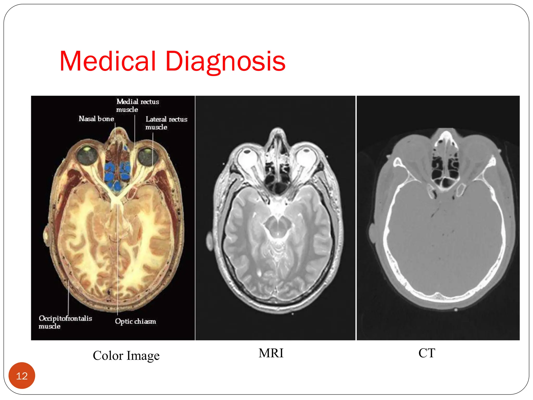
 Medicine: Medical diagnosis
 Retail: Market basket analysis, Customer relationship management (CRM)
 Finance: Credit scoring, fraud detection
 Manufacturing: Optimization, troubleshooting
 E-commerce
 Space exploration
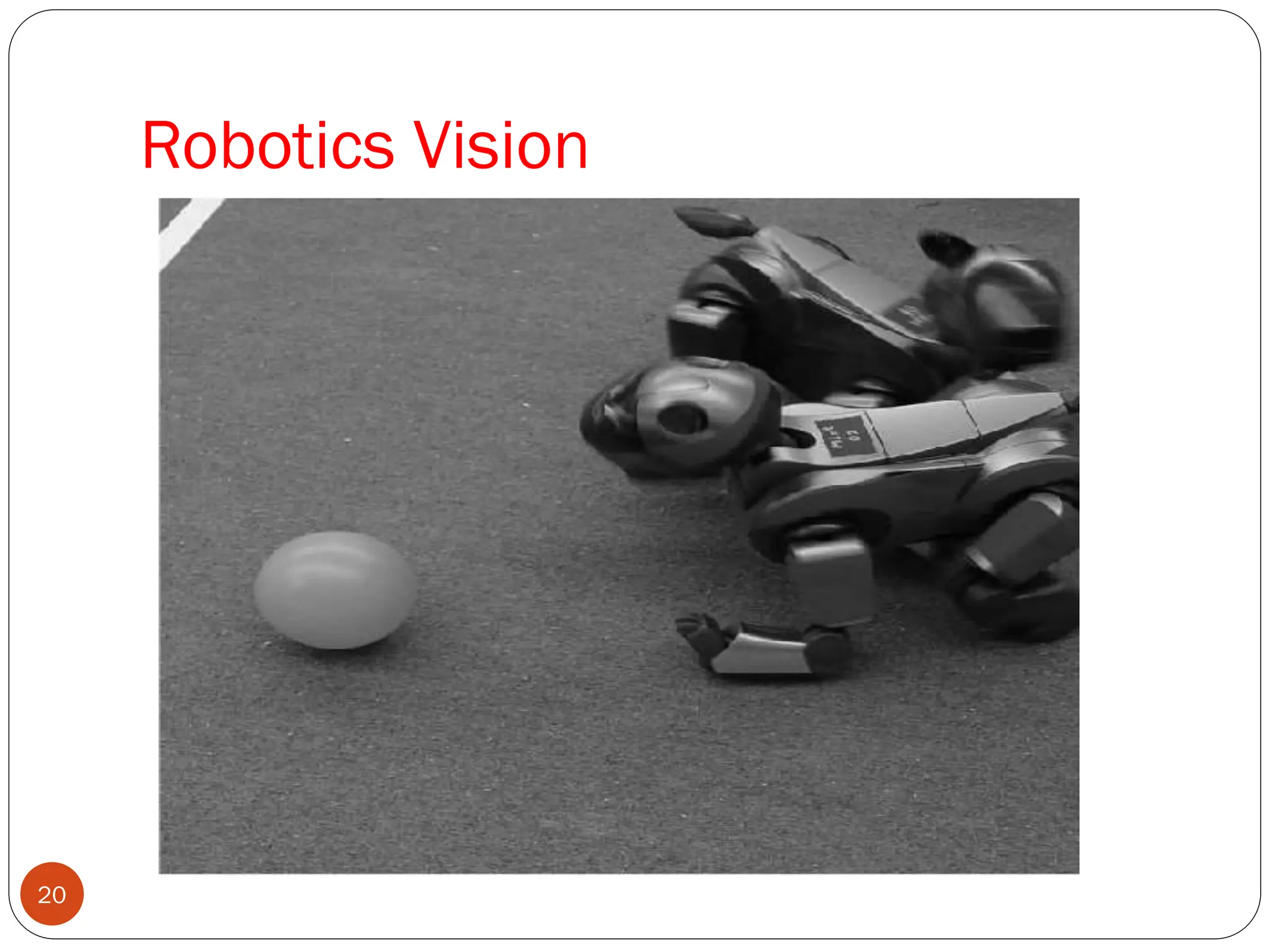
 Robotics
 Information extraction
 Social networks
 Debugging
 [Your favorite area]
Sample Applications
10

11. Drug Discovery
11

12. Medical Diagnosis
Color Image MRI CT
12

13. Iris Verification
13

14. Hand-written Digits Recognition
14

15. Radar Imaging
15

16. Speech Recognition
16

17. Signature Verification
17

18. Face Recognition
18

19. Target Recognition
19

20. Robotics Vision
20

21. Traffic Monitoring
21

22. ML in a Nutshell
 Tens of thousands of machine learning algorithms
 Hundreds new every year
 Every machine learning algorithm has three components:
 Representation
 Evaluation
 Optimization
22

23. Representation
 Decision trees
 Sets of rules / Logic programs
 Instances
 Graphical models (Bayes/Markov nets)
 Neural networks
 Support vector machines
 Model ensembles
 Etc.
23

24. Evaluation
 Accuracy
 Precision and recall
 Squared error
 Likelihood
 Posterior probability
 Cost / Utility
 Margin
 Entropy
 K-L divergence
 Etc.
24

25. Optimization
 Combinatorial optimization
 E.g.: Greedy search
 Convex optimization
 E.g.: Gradient descent
 Constrained optimization
 E.g.: Linear programming
25

26. Machine Learning Resources
• Data
– NIPS 2003 feature selection contest
– mldata.org
– UCI machine learning repository
– LIDC-IDRI (Lung Nodule/Tumor Images), MICCAI(Brain MRI Images)
• Contests
– Kaggle
• Software
– Python sci-kit
– R
– Tensorflow
– Keras, Pytorch
– Your own code
26

27. Machine Learning Steps
Problem Definition
Data Collection
Data Preprocessing
FEATURE EXTRACTION
Detection Classification Characterization
27

28. Example Pipeline.....
Image acquisition and pre-processing
Lung segmentation
Thorax extraction
Lung extraction
Nodule detection
Nodule candidate detection/ Tubular structure
elimination
Feature extraction/ False Positive reduction
Nodule Detection/Classification
Nodule Detection Framework
Problem Definition
Data Collection
Data Preprocessing
FEATURE
EXTRACTION
Detection Classification Characterization
28

29. Detection vs. Classification vs. Characterization
Typical SPNs for different type (a)Well-
circumscribed nodule, (b) Juxta-vascular nodule, (c)
Nodule with a pleural tail, (d) Juxta-pleural nodule
Benign Malignant
Characterization
Classification
Detection (Finding the location of the ROI)
29

30. Feature Extraction
1
Minor AxisValue
Elongation
Major AxisValue
  4
2
Area
Cir
Perimeter



Area of Object
Ext
Areaof theBounding Box

30

31. What about GGO nodule?
31

32. 32

33.  Given examples of a function (X,F(X))
 Predict function F(X) for new examples X
 Discrete F(X): Classification
 Continuous F(X): Regression
 F(X) = Probability(X): Probability estimation
Inductive Learning
33

34. 34

35. 35

36. 36

37. 37

38. Supervised Learning
 Regression is used for ContinuousTargetValue
 Classification is used for discreteTargetValue(Class
Label)
Supervised Learning
Regression Classification
38

39. Regression
 Regression is used for ContinuousTargetValue
 Classification is used for discreteTargetValue(Class
Label)
Regression
Logistics
Linear
39

40.  In machine learning, a regression problem is the problem of
predicting the value of a numeric variable based on observed
values of the variable.
 These are often quantities, such as amounts and sizes.
Brain
(in standard units)
Height
(in inches)
Weight
(in Pounds)
IQ Score
(in appropriate scales)
81.69 64.5 118 124
103.84 73.3 143 150
96.54 68.8 172 128
95.15 65.0 147 134
92.88 69.0 146 110
99.13 64.5 138 131
85.43 66.0 175 98
90.49 66.3 134 84
95.55 68.8 172 147
83.39 64.5 118 124
40

41. Linear
41

42. Logistic
 Linear regression + Sigmoid function
 Logistic regression is used when the dependent variable is
binary (0/1,True/False,Yes/No) in nature.
42

43. 43

44. Classification
 A classification problem requires that examples be classified
into one of two or more classes.
 A problem with two classes is often called a two-class or
binary classification problem.
 A problem with more than two classes is often called a multi-
class classification problem.
 A problem where an example is assigned multiple classes is
called a multi-label classification problem.
44

45.  Binary Classification: This is the most basic type of
classification. In this case, an input is classified into one of
two possible categories. For example, a common application
of binary classification is in determining whether an animal is
a 'cat' or a 'dog'.
45

46.  Multiclass Classification: This type of classification
involves classifying an input into one of three or more
categories. An example of this is the identifying image, where
an image can be classified as a train, ship, bus, or airplane,
thus involving four different classes.
46

47.  Imbalanced Classification: This is a specialized form of
classification where the classes are not equally distributed. It's
often found in real-world scenarios where one class
significantly outnumbers the other. For example, in
identifying manufacturing defects, the 'defective' class is
usually outnumbered by the 'non-defective' class.
47

48.  Multilabel Classification: This is a more complex
scenario where an input can be associated with multiple
labels e.g.,
 In a movie recommendation system, a single movie could be
tagged with several genres, such as 'action', 'adventure', and
'sci-fi'.
 An image can contain multiple objects, as illustrated below:
the model predicted that the image contains: a plane, a boat,
a truck, and a dog.
48

49. 49

50. Classifier
 Naive Bayes Classifier
 Nearest Neighbor Classifier
 DecisionTree
50

51. Linear Versus Non Linear Boundary
51

52. Bayes’ Theorem
 A is called the proposition and B is called the evidence.
 P(A) is called the prior probability of proposition and P(B)
is called the prior probability of evidence.
 P(A|B ) is called the posterior probability of A given B.
 P(B|A) is called the likelihood of B given A.
52

53.  In General.......
53

54. Naive Bayes Classifier
Sl.
No.
Swim Fly Crawl Class
1 Fast No No Fish
2 Fast No Yes Animal
3 Slow No No Animal
4 Fast No No Animal
5 No Short No Bird
6 No Short No Bird
7 No Rarely No Animal
8 Slow No Yes Animal
9 Slow No No Fish
10 Slow No Yes Fish
11 No Long No Bird
12 Fast No No Bird
54

55. •P(c|x) is the posterior probability of class (target) given predictor (attribute).
•P(c) is the prior probability of class.
•P(x|c) is the likelihood which is the probability of predictor given class.
•P(x) is the prior probability of predictor.
55

56. Sl. No. Swim Fly Crawl Class
1 Fast No No Fish
2 Fast No Yes Animal
3 Slow No No Animal
4 Fast No No Animal
5 No Short No Bird
6 No Short No Bird
7 No Rarely No Animal
8 Slow No Yes Animal
9 Slow No No Fish
10 Slow No Yes Fish
11 No Long No Bird
12 Fast No No Bird
Feature
Name
Value
Swim Fast, Slow, No
Fly
Long, Short, Rarely,
No
Crawl Yes, No
Use naive Bayes algorithm to
classify a particular species if its
features (X)=(Slow, Rarely, No)?
Example
56

57. Class
Features
Total
Swim (F1) Fly (F2) Craw (F3)
Fast Slow No Long Short Rarely No Yes No
Animal (c1) 2 2 1 0 0 1 4 2 3 5
Bird (c2) 1 0 3 1 2 0 1 1 3 4
Fish (c3) 1 2 0 0 0 0 3 0 3 3
Total 4 4 4 1 2 1 8 3 9 12
57

58. Class
Features
Swim (F1) Fly (F2) Craw (F3)
Fast Slow No Long Short Rarely No Yes No
Animal (c1) 2/5 2/5 1/5 0/5 0/5 1/5 4/5 2/5 3/5
Bird (c2) 1/4 0/4 3/4 1/4 2/4 0/4 1/4 1/4 3/4
Fish (c3) 1/3 2/3 0/3 0/3 0/3 0/3 3/3 0/3 3/3
58

59. max{q1, q2, q3} = 0.02.
59

60. Nearest Neighbor Classifier
60

61. Apply KNN with K=3
Output
61

62. BRIGHTNESS (X) SATURATION (Y) CLASS LABEL
40 20 Red
50 50 Blue
60 90 Blue
10 25 Red
70 70 Blue
60 10 Red
25 80 Blue
BRIGHTNESS
(Xtest)
SATURATION
(Ytest)
CLASS LABEL
20 35 ?
   
2 2
i test i test
d x x y y
   
d1 = √(20 - 40)² + (35 - 20)²
= √400 + 225
= √625
= 25
62

63. BRIGHTNESS
(X)
SATURATION
(Y)
CLASS
LABEL
DISTANCE
40 20 Red 25
50 50 Blue ?
60 90 Blue ?
10 25 Red ?
70 70 Blue ?
60 10 Red ?
25 80 Blue ?
BRIGHTNESS
(X)
SATURATION
(Y)
CLASS
LABEL
DISTANCE
40 20 Red 25
50 50 Blue 33.54
60 90 Blue ?
10 25 Red ?
70 70 Blue ?
60 10 Red ?
25 80 Blue ?
BRIGHTNESS
(X)
SATURATION
(Y)
CLASS DISTANCE
40 20 Red 25
50 50 Blue 33.54
60 90 Blue 68.01
10 25 Red 10
70 70 Blue 61.03
60 10 Red 47.17
25 80 Blue 45
BRIGHTNESS
(X)
SATURATION
(Y)
CLASS DISTANCE
10 25 Red 10
40 20 Red 25
50 50 Blue 33.54
25 80 Blue 45
60 10 Red 47.17
70 70 Blue 61.03
60 90 Blue 68.01
Sort the
dataset in
descending
order
Choose top 5 rows (K=5)
and find the maximum
class labels.
63

64. Decision Tree
64

65. 65

66. Entropy:
 Entropy is a measure of disorder or impurity in the given
dataset.
 It returns us the information about an arbitrary dataset that
how impure/non-homogeneous the data set is.
Selection of Splitting Attribute in
Decision Tree
66

67. 67

68. Information Gain:
 The Information Gain measures the expected reduction in
entropy.
 The feature which has minimum impurity will be considered as
the root node.
 Information gain is used to decide which feature to split on at each
step in building the tree.
 Information gain of a parent node can be calculated as the entropy
of the parent node subtracted entropy of the weighted average of
the child node.
 For a dataset having many features, the information gain of each
feature is calculated. The feature having maximum information
gain will be the most important feature which will be the root
node for the decision tree.
68

69. 69

70. 70

71. 71

72. Gini Index:
 The Gini index can also be used for feature selection.
 The tree chooses the feature that minimizes the Gini
impurity index.
 The higher value of the Gini Index indicates the impurity is
higher.
72

73. 73

74. 74

75. Finally, let = Soutlook = rain.The highest information gain for this data set is
Gain(S(2); humidity).The branches resulting from splitting this node corresponding to the
values “high” and “normal” of “humidity” lead to leaf nodes with class labels “no” and ”yes”.
With these changes, we get the tree in Figure 8.10.
(2)
S
75

76. Support Vector Machine
Linear
Non Linear
76

77.  Hyperplane:
A hyperplane is a decision boundary which separates
between given set of data points having different class labels.
The SVM classifier separates data points using a hyperplane
with the maximum amount of margin. This hyperplane is
known as the maximum margin hyperplane and the linear
classifier it defines is known as the maximum margin
classifier.
77

78.  SupportVectors:
Support vectors are the sample data points, which are closest
to the hyperplane. These data points will define the
separating line or hyperplane better by calculating margins.
 Margin:
A margin is a separation gap between the two lines on the
closest data points. It is calculated as the perpendicular
distance from the line to support vectors or closest data
points. In SVMs, we try to maximize this separation gap so
that we get maximum margin.
78

79. 79

80. Kernel Functions for SVM
 Kernel: Kernel is the mathematical function, which is used in SVM to map the
original input data points into high-dimensional feature spaces, so, that the
hyperplane can be easily found out even if the data points are not linearly
separable in the original input space. Some of the common kernel functions are
linear, polynomial, radial basis function(RBF), and sigmoid.
80

81. 81

82. 82

83. 83

84. Overfitting and Underfitting
84

85. How Do We Learn?
Human Machine
Memorize k-Nearest Neighbors,
Case-based learning
Observe someone else, then
repeat
Supervised Learning,
Learning by Demonstration
Keep trying until it works
(riding a bike)
Reinforcement Learning
20 Questions Decision Tree
Pattern matching (faces,
voices, languages)
Pattern Recognition
Guess that current trend will
continue (stock market, real
estate prices)
Regression
85

86. Reference Books
 R. Duda, P. Hart & D. Stork, Pattern Classification (2nd ed.),
Wiley (Required)
 T. Mitchell, Machine Learning,McGraw-Hill(Recommended)
 Introduction to Machine Learning by Ethem Alpaydin (2nd edition,
2010, MIT Press).Written by computer scientist and material is
accessible with basic probability and linear algebra background
 Foundations of Machine Learning by Afshin Rostamizadeh,Ameet
Talwalkar, and Mehryar Mohri (2012, MIT Press)
 Learning with Kernels by Scholkopf and Smola (2001, MIT Press)
 Applied predictive modeling by Kuhn and Johnson (2013, Springer).
This book focuses on practical modeling.
86

87. About Me
 Dr.Amitava Halder
B.Tech. (Wbut), M.Tech. (IIEST formerly BESU), Ph.D.
(Jadavpur University)
 Contact Information:
9831402704/9073310777
 Mail Id: amitava.halder2008@gmail.com
 Google Scholar Id: J-kPvN8AAAAJ
 Research Domain/Interest: Image Processing, Biomedical
Image Processing, Machine Learning, Deep Learning, Pattern
Recognition.
Please cite my works available at Google Scholar!!
87

88. 88

89. 89