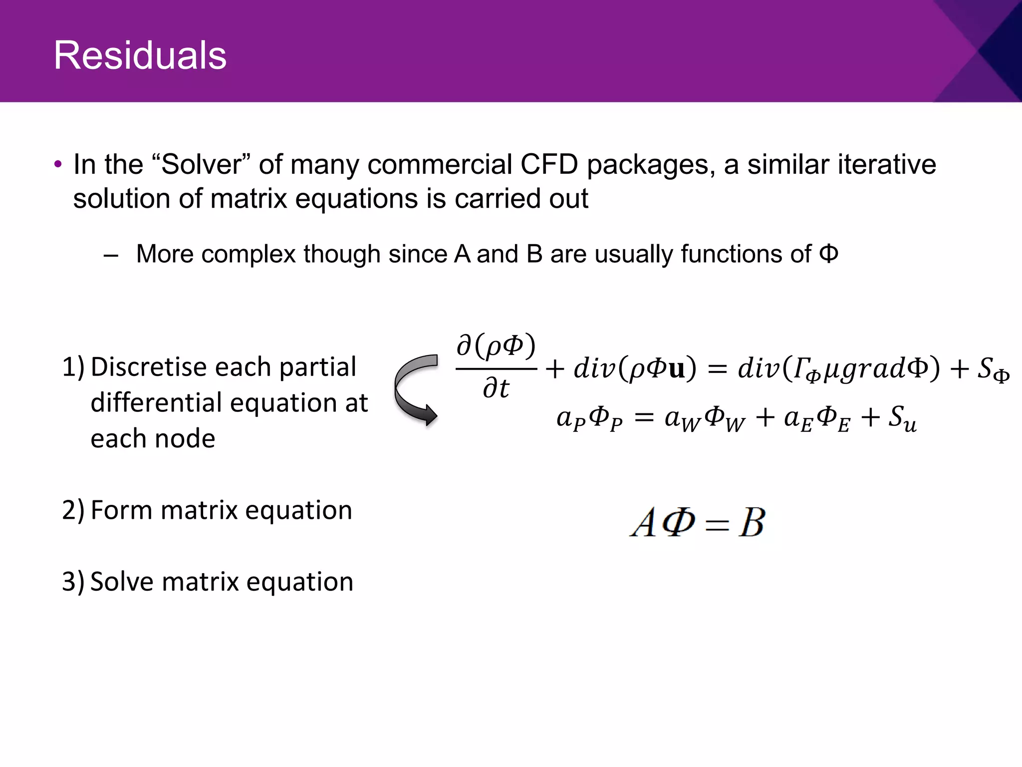
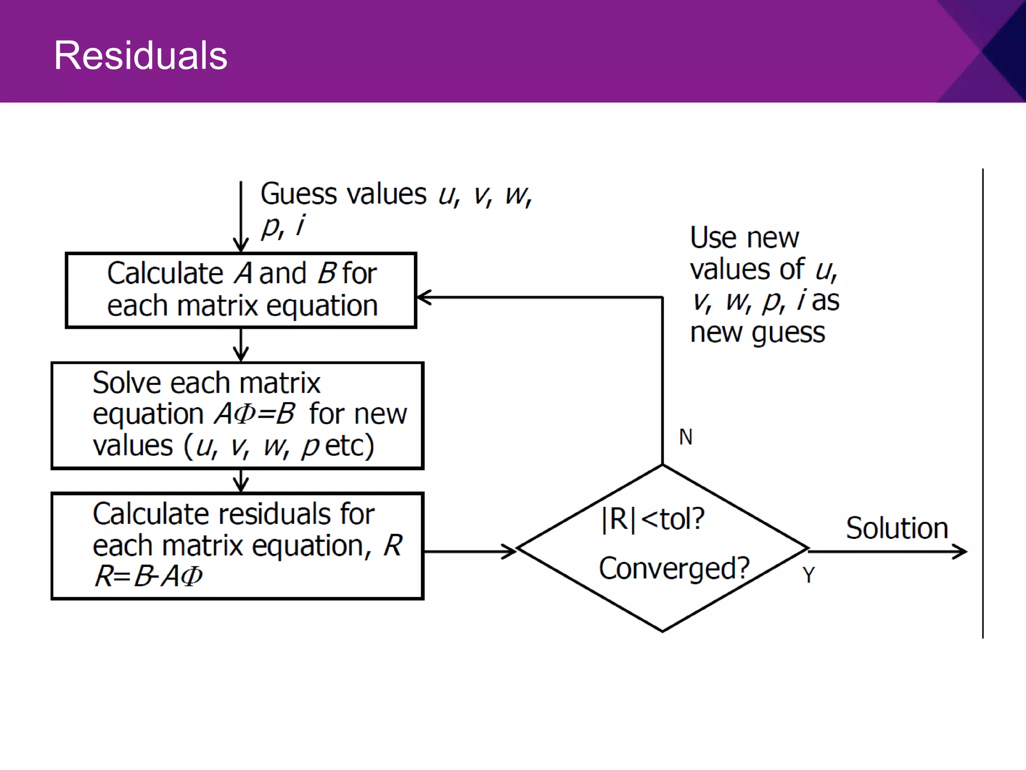
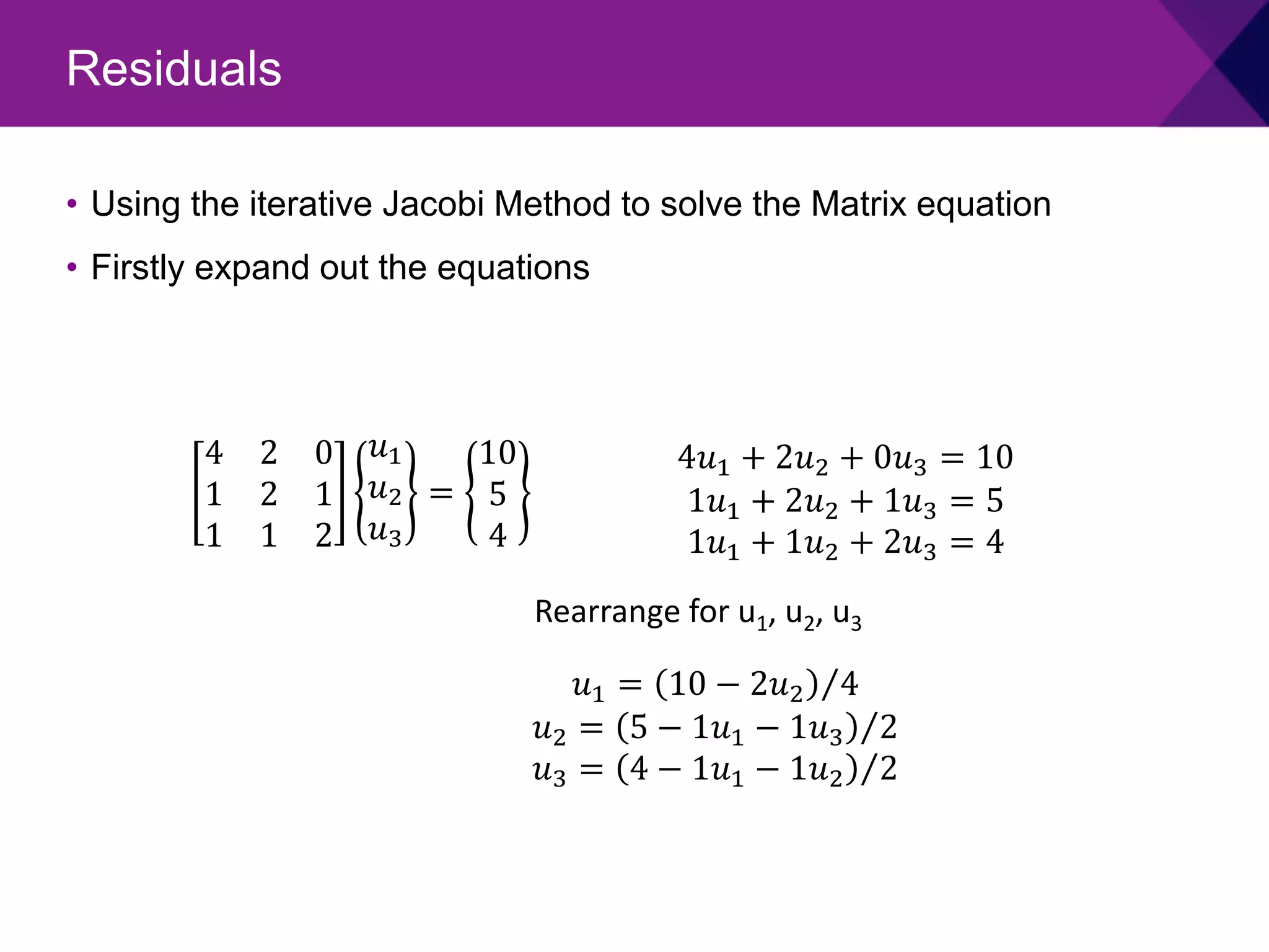
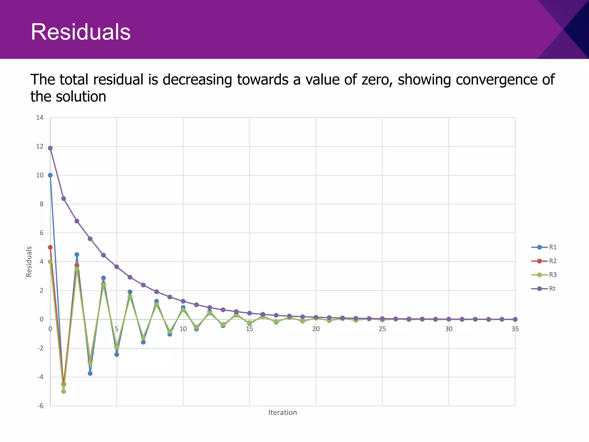
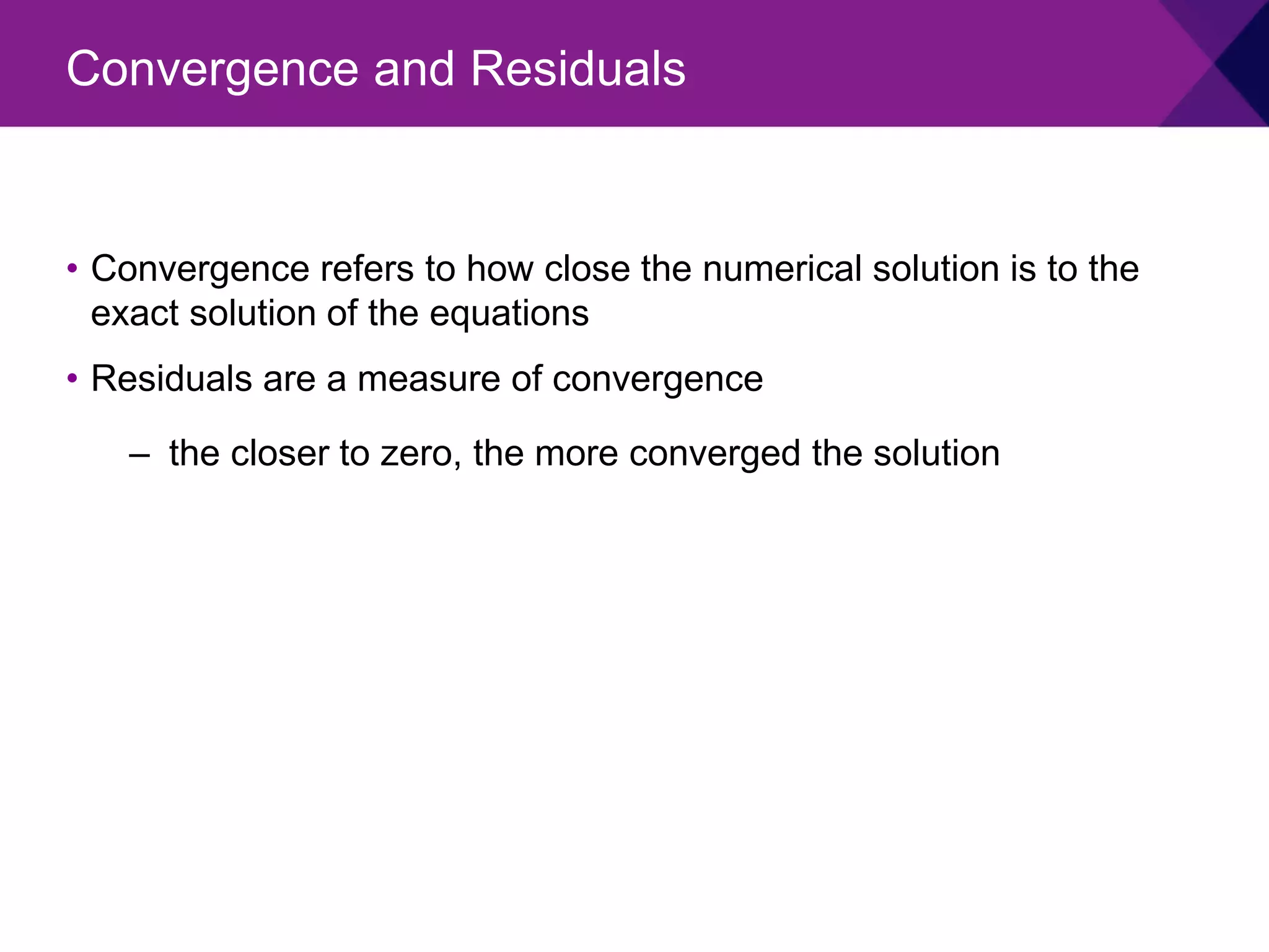
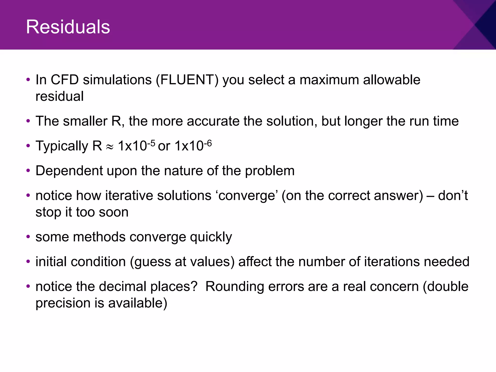
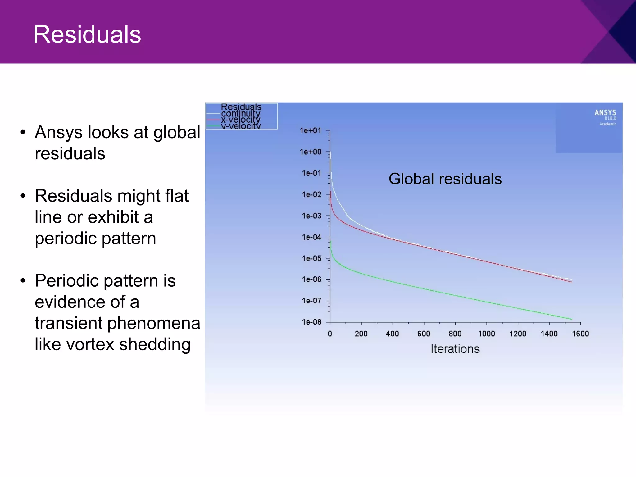
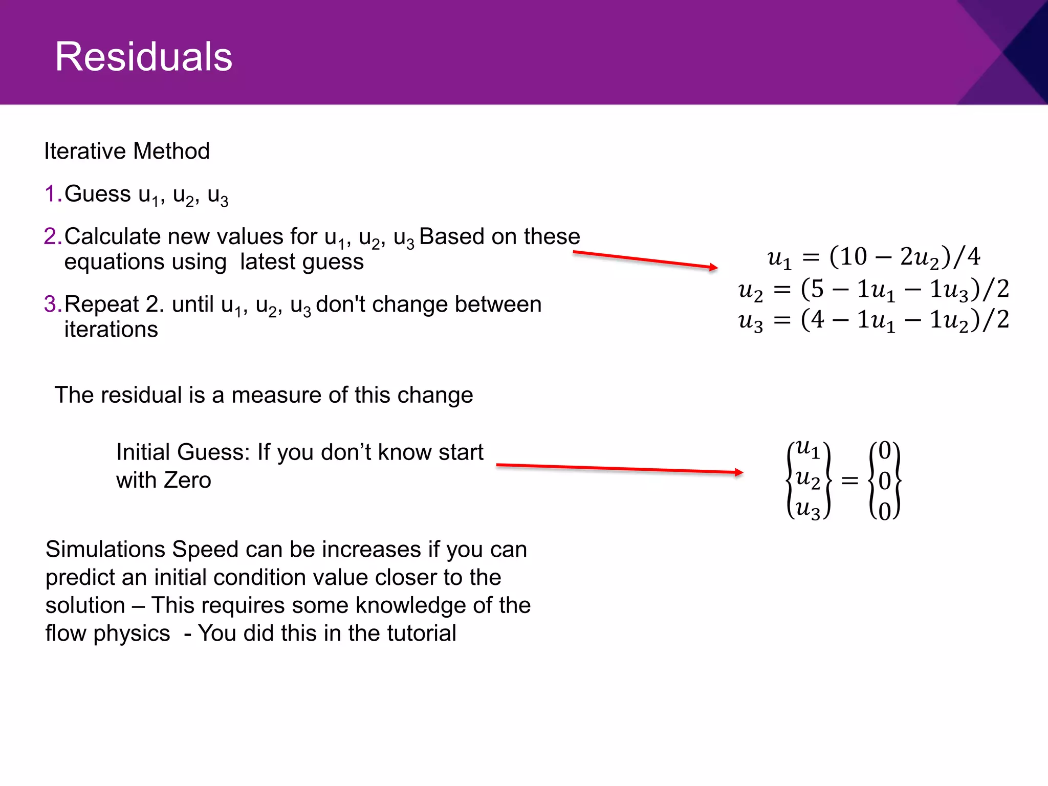
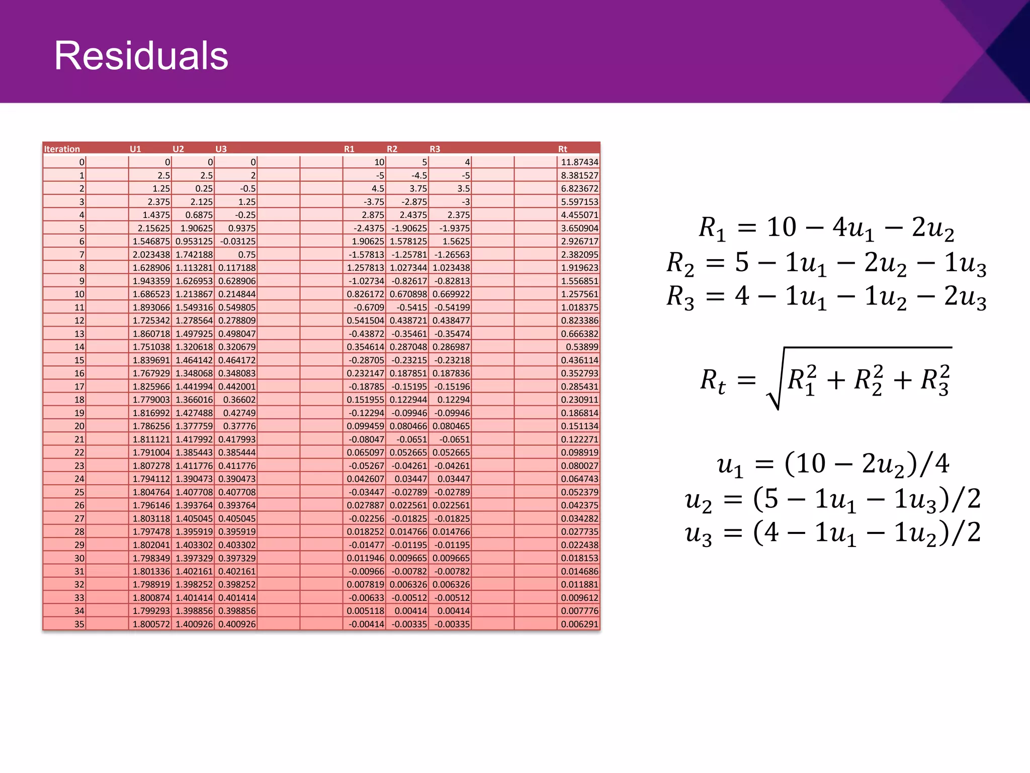
- The document discusses using the iterative Jacobi method to solve a matrix equation representing a computational fluid dynamics (CFD) problem. - Residuals are calculated at each iteration to measure how well the current solution satisfies the matrix equation, with residuals approaching zero indicating convergence of the solution. - After 35 iterations, the Jacobi method solution converged to u1=1.801, u2=1.401, u3=0.4, matching the analytical solution from Excel.

1. Dr Patrick Geoghegan
Book: H. Versteeg and W. Malalasekera An Introduction to
Computational Fluid Dynamics: The Finite Volume Method
FEA/CFD for
Biomedical
Engineering
Week 10: CFD

2. Residuals

3. Lets demonstrate this through an example
We will solve this matrix equation using the iterative Jacobi Method
Residuals
4 2 0
1 2 1
1 1 2
𝑢𝑢1
𝑢𝑢2
𝑢𝑢3
=
10
5
4
}
{
}
]{
[ F
u
K =
}
{
]
[
}
{ 1
F
K
u −
=
Using the Excel Function
=MMULT(MINVERSE(B2:D4),(F2:F4))
𝑢𝑢1
𝑢𝑢2
𝑢𝑢3
=
1.8
1.4
0.4

4. • Using the iterative Jacobi Method to solve the Matrix equation
• Firstly expand out the equations
Residuals
4𝑢𝑢1 + 2𝑢𝑢2 + 0𝑢𝑢3 = 10
1𝑢𝑢1 + 2𝑢𝑢2 + 1𝑢𝑢3 = 5
1𝑢𝑢1 + 1𝑢𝑢2 + 2𝑢𝑢3 = 4
4 2 0
1 2 1
1 1 2
𝑢𝑢1
𝑢𝑢2
𝑢𝑢3
=
10
5
4
𝑢𝑢1 = ⁄
10 − 2𝑢𝑢2 4
𝑢𝑢2 = ⁄
5 − 1𝑢𝑢1 − 1𝑢𝑢3 2
𝑢𝑢3 = ⁄
4 − 1𝑢𝑢1 − 1𝑢𝑢2 2
Rearrange for u1, u2, u3

5. • Residuals tell us whether or not the values u1, u2 and u3 satisfy the
matrix equation
Residuals
4𝑢𝑢1 + 2𝑢𝑢2 + 0𝑢𝑢3 = 10
1𝑢𝑢1 + 2𝑢𝑢2 + 1𝑢𝑢3 = 5
1𝑢𝑢1 + 1𝑢𝑢2 + 2𝑢𝑢3 = 4
4 2 0
1 2 1
1 1 2
𝑢𝑢1
𝑢𝑢2
𝑢𝑢3
=
10
5
4
𝑅𝑅1 = 10 − 4𝑢𝑢1 − 2𝑢𝑢2
𝑅𝑅2 = 5 − 1𝑢𝑢1 − 2𝑢𝑢2 − 1𝑢𝑢3
𝑅𝑅3 = 4 − 1𝑢𝑢1 − 1𝑢𝑢2 − 2𝑢𝑢3
They are calculated as follows
The equations are satisfied
when these equal zero

6. Iterative Method
1.Guess u1, u2, u3
2.Calculate new values for u1, u2, u3 Based on these
equations using latest guess
3.Repeat 2. until u1, u2, u3 don't change between
iterations
Residuals
𝑢𝑢1 = ⁄
10 − 2𝑢𝑢2 4
𝑢𝑢2 = ⁄
5 − 1𝑢𝑢1 − 1𝑢𝑢3 2
𝑢𝑢3 = ⁄
4 − 1𝑢𝑢1 − 1𝑢𝑢2 2
𝑢𝑢1
𝑢𝑢2
𝑢𝑢3
=
0
0
0
Initial Guess: If you don’t know start
with Zero
The residual is a measure of this change
Simulations Speed can be increases if you can
predict an initial condition value closer to the
solution – This requires some knowledge of the
flow physics - You did this in the tutorial

7. Iteration U1 U2 U3 R1 R2 R3 Rt
0 0 0 0 10 5 4 11.87434
1 2.5 2.5 2 -5 -4.5 -5 8.381527
2 1.25 0.25 -0.5 4.5 3.75 3.5 6.823672
3 2.375 2.125 1.25 -3.75 -2.875 -3 5.597153
4 1.4375 0.6875 -0.25 2.875 2.4375 2.375 4.455071
5 2.15625 1.90625 0.9375 -2.4375 -1.90625 -1.9375 3.650904
6 1.546875 0.953125 -0.03125 1.90625 1.578125 1.5625 2.926717
7 2.023438 1.742188 0.75 -1.57813 -1.25781 -1.26563 2.382095
8 1.628906 1.113281 0.117188 1.257813 1.027344 1.023438 1.919623
9 1.943359 1.626953 0.628906 -1.02734 -0.82617 -0.82813 1.556851
10 1.686523 1.213867 0.214844 0.826172 0.670898 0.669922 1.257561
11 1.893066 1.549316 0.549805 -0.6709 -0.5415 -0.54199 1.018375
12 1.725342 1.278564 0.278809 0.541504 0.438721 0.438477 0.823386
13 1.860718 1.497925 0.498047 -0.43872 -0.35461 -0.35474 0.666382
14 1.751038 1.320618 0.320679 0.354614 0.287048 0.286987 0.53899
15 1.839691 1.464142 0.464172 -0.28705 -0.23215 -0.23218 0.436114
16 1.767929 1.348068 0.348083 0.232147 0.187851 0.187836 0.352793
17 1.825966 1.441994 0.442001 -0.18785 -0.15195 -0.15196 0.285431
18 1.779003 1.366016 0.36602 0.151955 0.122944 0.12294 0.230911
19 1.816992 1.427488 0.42749 -0.12294 -0.09946 -0.09946 0.186814
20 1.786256 1.377759 0.37776 0.099459 0.080466 0.080465 0.151134
21 1.811121 1.417992 0.417993 -0.08047 -0.0651 -0.0651 0.122271
22 1.791004 1.385443 0.385444 0.065097 0.052665 0.052665 0.098919
23 1.807278 1.411776 0.411776 -0.05267 -0.04261 -0.04261 0.080027
24 1.794112 1.390473 0.390473 0.042607 0.03447 0.03447 0.064743
25 1.804764 1.407708 0.407708 -0.03447 -0.02789 -0.02789 0.052379
26 1.796146 1.393764 0.393764 0.027887 0.022561 0.022561 0.042375
27 1.803118 1.405045 0.405045 -0.02256 -0.01825 -0.01825 0.034282
28 1.797478 1.395919 0.395919 0.018252 0.014766 0.014766 0.027735
29 1.802041 1.403302 0.403302 -0.01477 -0.01195 -0.01195 0.022438
30 1.798349 1.397329 0.397329 0.011946 0.009665 0.009665 0.018153
31 1.801336 1.402161 0.402161 -0.00966 -0.00782 -0.00782 0.014686
32 1.798919 1.398252 0.398252 0.007819 0.006326 0.006326 0.011881
33 1.800874 1.401414 0.401414 -0.00633 -0.00512 -0.00512 0.009612
34 1.799293 1.398856 0.398856 0.005118 0.00414 0.00414 0.007776
35 1.800572 1.400926 0.400926 -0.00414 -0.00335 -0.00335 0.006291
Residuals
𝑅𝑅𝑡𝑡 = 𝑅𝑅1
2
+ 𝑅𝑅2
2
+ 𝑅𝑅3
2
𝑅𝑅1 = 10 − 4𝑢𝑢1 − 2𝑢𝑢2
𝑅𝑅2 = 5 − 1𝑢𝑢1 − 2𝑢𝑢2 − 1𝑢𝑢3
𝑅𝑅3 = 4 − 1𝑢𝑢1 − 1𝑢𝑢2 − 2𝑢𝑢3
𝑢𝑢1 = ⁄
10 − 2𝑢𝑢2 4
𝑢𝑢2 = ⁄
5 − 1𝑢𝑢1 − 1𝑢𝑢3 2
𝑢𝑢3 = ⁄
4 − 1𝑢𝑢1 − 1𝑢𝑢2 2

8. -1
-0.5
0
0.5
1
1.5
2
2.5
3
0 5 10 15 20 25 30 35
Velocity
Iteration
U1
U2
U3
Residuals
The Jacobi Method gives a solution of
in 35 iterations
Excel gives a solution of [1.8,1.4,0.4]
𝑢𝑢1
𝑢𝑢2
𝑢𝑢3
=
1.801
1.401
0.4

9. -6
-4
-2
0
2
4
6
8
10
12
14
0 5 10 15 20 25 30 35
Residuals
Iteration
R1
R2
R3
Rt
Residuals
The total residual is decreasing towards a value of zero, showing convergence of
the solution

10. • Convergence refers to how close the numerical solution is to the
exact solution of the equations
• Residuals are a measure of convergence
– the closer to zero, the more converged the solution
Convergence and Residuals

11. Residuals in CFD

12. • Imagine a geometry as shown below that is divided into discrete control
volumes with nodes at centre
Residuals

13. Φ=1 for conservation of mass
Φ =u for conservation of x-momentum
Φ =v for conservation of y-momentum
Φ =w for conservation of z-momentum
Φ =i for conservation of internal energy
• Any terms that are not in the common form have been hidden within the source
terms
• For example Γ diffusive term represents μ for the momentum equations
The General Transport Equation
𝜕𝜕 𝜌𝜌𝛷𝛷
𝜕𝜕𝜕𝜕
+ 𝑑𝑑𝑑𝑑𝑑𝑑 𝜌𝜌𝜌𝜌𝐮𝐮 = 𝑑𝑑𝑑𝑑𝑑𝑑 𝛤𝛤
𝛷𝛷𝜇𝜇𝑔𝑔𝑔𝑔𝑔𝑔𝑔𝑔Φ + 𝑆𝑆Φ

14. • In the “Solver” of many commercial CFD packages, a similar iterative
solution of matrix equations is carried out
– More complex though since A and B are usually functions of Φ
Residuals
1) Discretise each partial
differential equation at
each node
2) Form matrix equation
3) Solve matrix equation
𝜕𝜕 𝜌𝜌𝛷𝛷
𝜕𝜕𝜕𝜕
+ 𝑑𝑑𝑑𝑑𝑑𝑑 𝜌𝜌𝜌𝜌𝐮𝐮 = 𝑑𝑑𝑑𝑑𝑑𝑑 𝛤𝛤
𝛷𝛷𝜇𝜇𝑔𝑔𝑔𝑔𝑔𝑔𝑔𝑔Φ + 𝑆𝑆Φ
𝑎𝑎𝑃𝑃𝛷𝛷𝑃𝑃 = 𝑎𝑎𝑊𝑊𝛷𝛷𝑊𝑊 + 𝑎𝑎𝐸𝐸𝛷𝛷𝐸𝐸 + 𝑆𝑆𝑢𝑢

15. • One such matrix equation for each variable (u, v, w, p etc)
• A and B are usually functions of velocity, pressure, temperature etc
need iterative solution
(1)Use estimates of u, v, w, p, T to calculate A and B
(2)Solve matrix equations for new u, v, w, p, T
(3)Iterate until convergence is achieved
Residuals

16. Residuals

17. • In CFD simulations (FLUENT) you select a maximum allowable
residual
• The smaller R, the more accurate the solution, but longer the run time
• Typically R ≈ 1x10-5 or 1x10-6
• Dependent upon the nature of the problem
• notice how iterative solutions ‘converge’ (on the correct answer) – don’t
stop it too soon
• some methods converge quickly
• initial condition (guess at values) affect the number of iterations needed
• notice the decimal places? Rounding errors are a real concern (double
precision is available)
Residuals

18. Residuals
• Ansys looks at global
residuals
• Residuals might flat
line or exhibit a
periodic pattern
• Periodic pattern is
evidence of a
transient phenomena
like vortex shedding
Global residuals