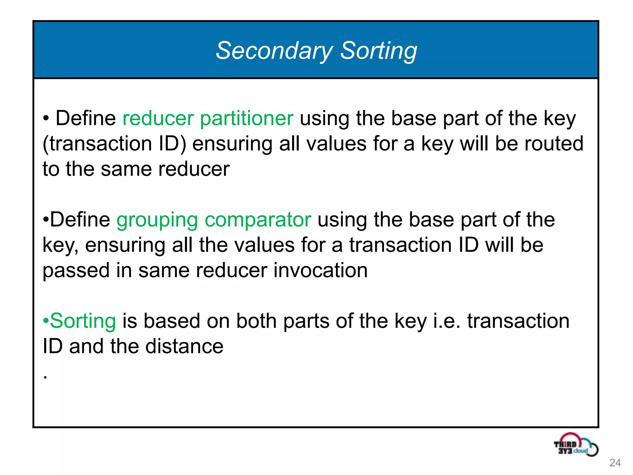
Downloaded 441 times


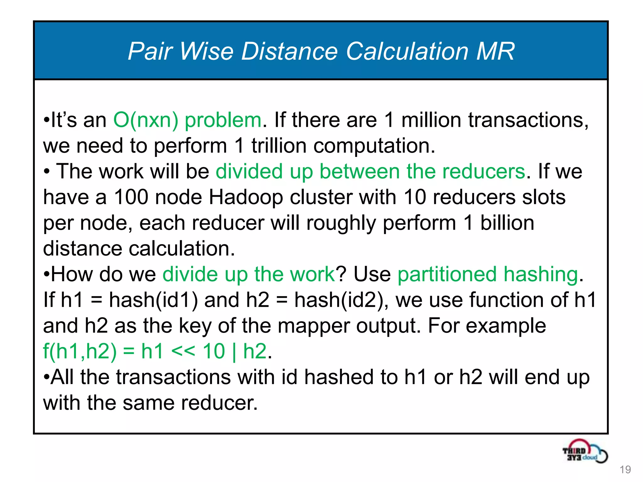
![Partitioned Hashing
• Code snippet from SameTypeSimilarity.java
String partition = partitonOrdinal>= 0 ? items[partitonOrdinal] : "none";
hash = (items[idOrdinal].hashCode() % bucketCount + bucketCount) / 2 ;
for (inti = 0; i<bucketCount; ++i) {
if (i< hash){
hashPair = hash * 1000 + i;
keyHolder.set(partition, hashPair,0);
valueHolder.set("0" + value.toString());
} else {
hashPair = i * 1000 + hash;
keyHolder.set(partition, hashPair,1);
valueHolder.set("1" + value.toString());
}
context.write(keyHolder, valueHolder);
20](https://image.slidesharecdn.com/outlierandfrauddetection-120722200508-phpapp02/75/Outlier-and-fraud-detection-using-Hadoop-20-2048.jpg)

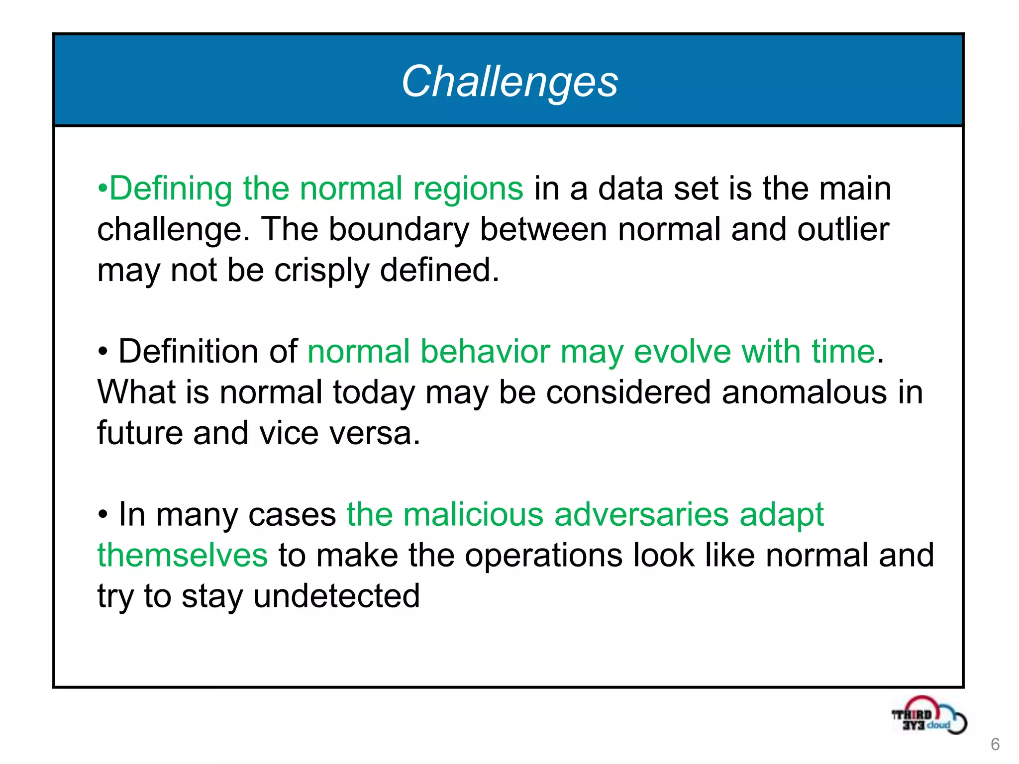
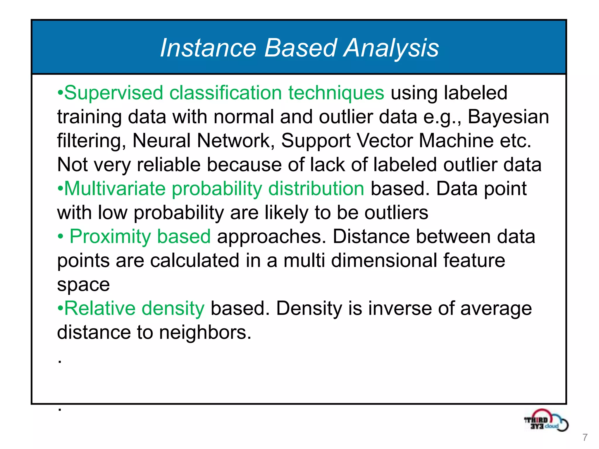
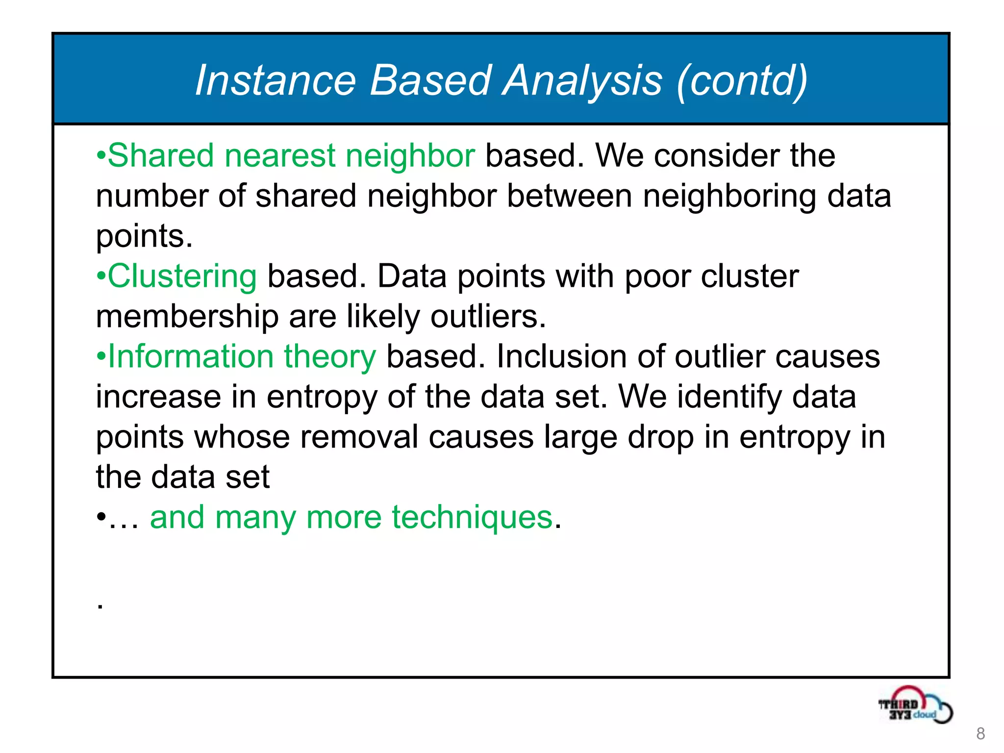
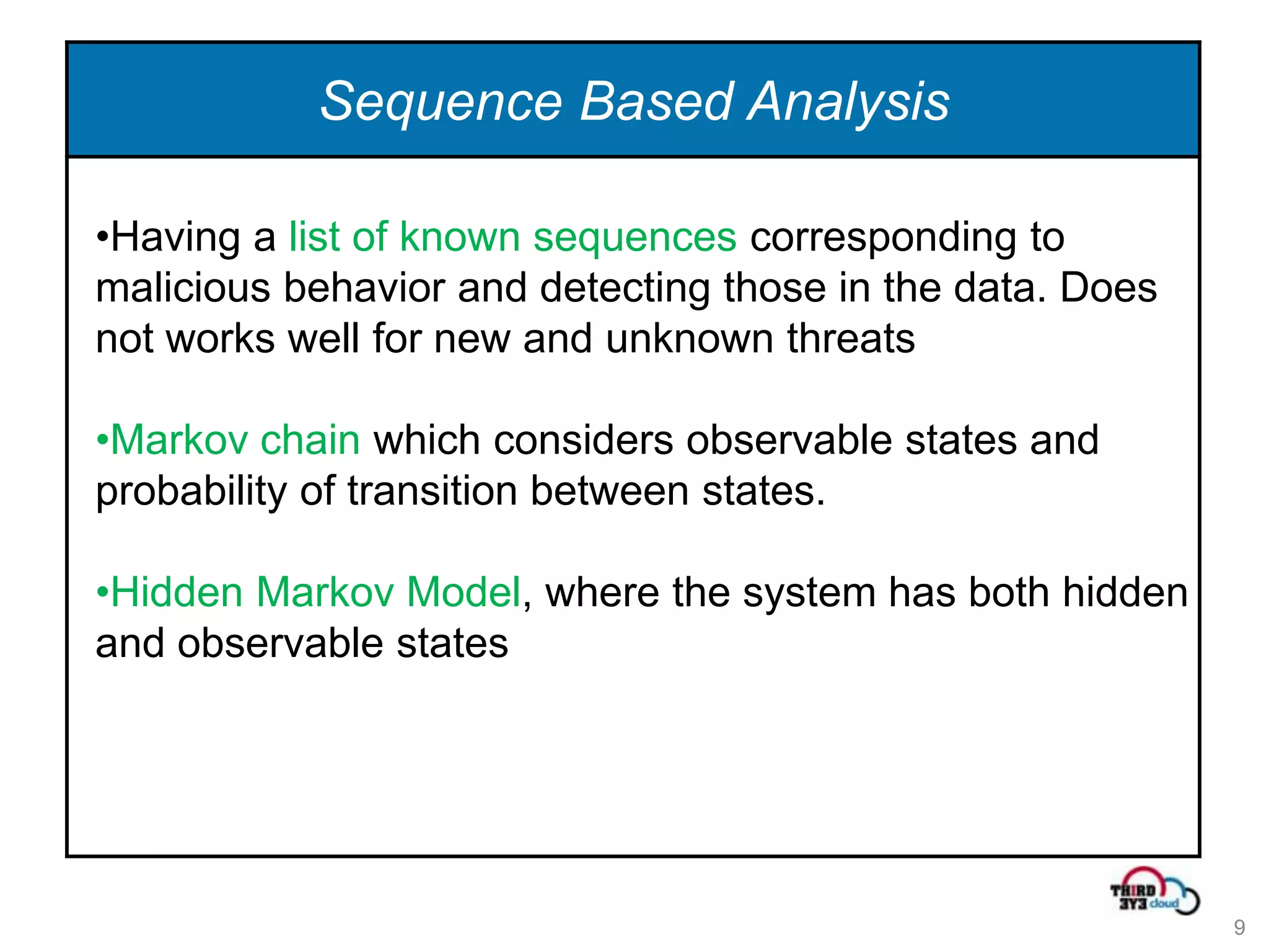
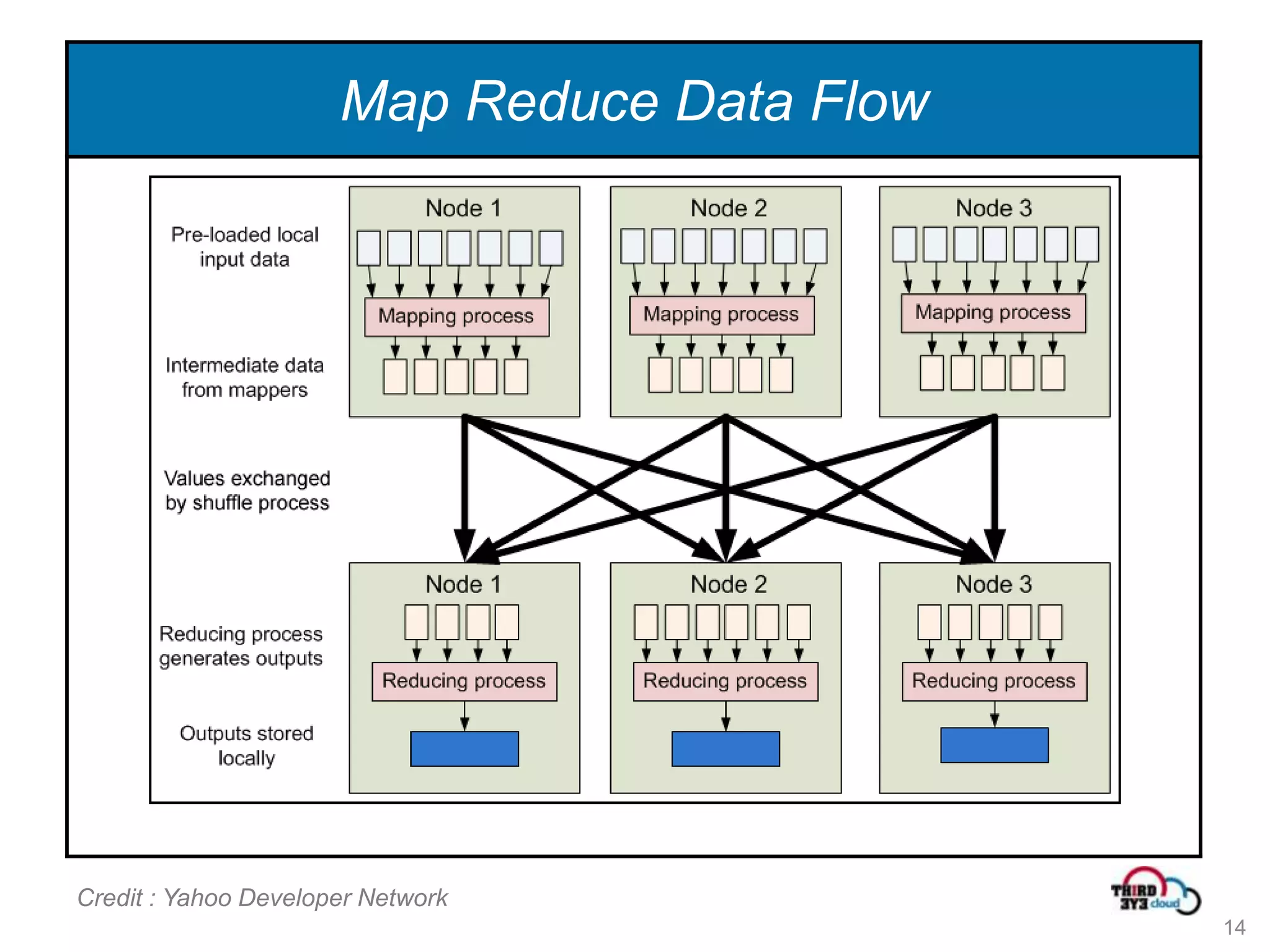
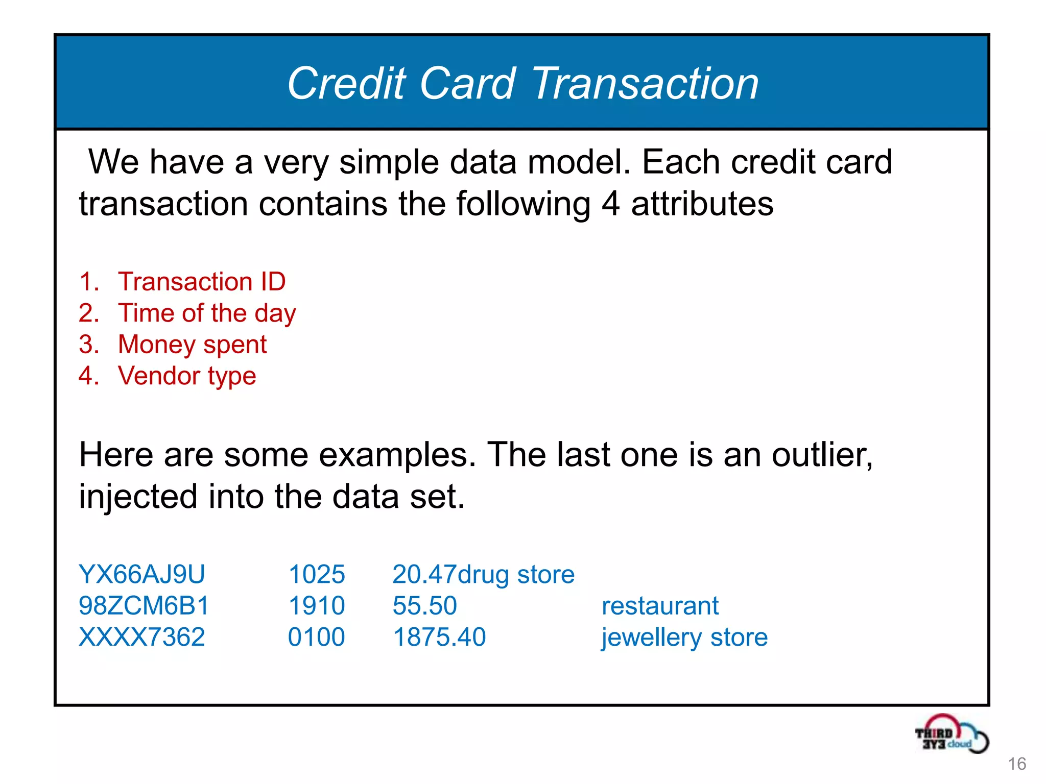
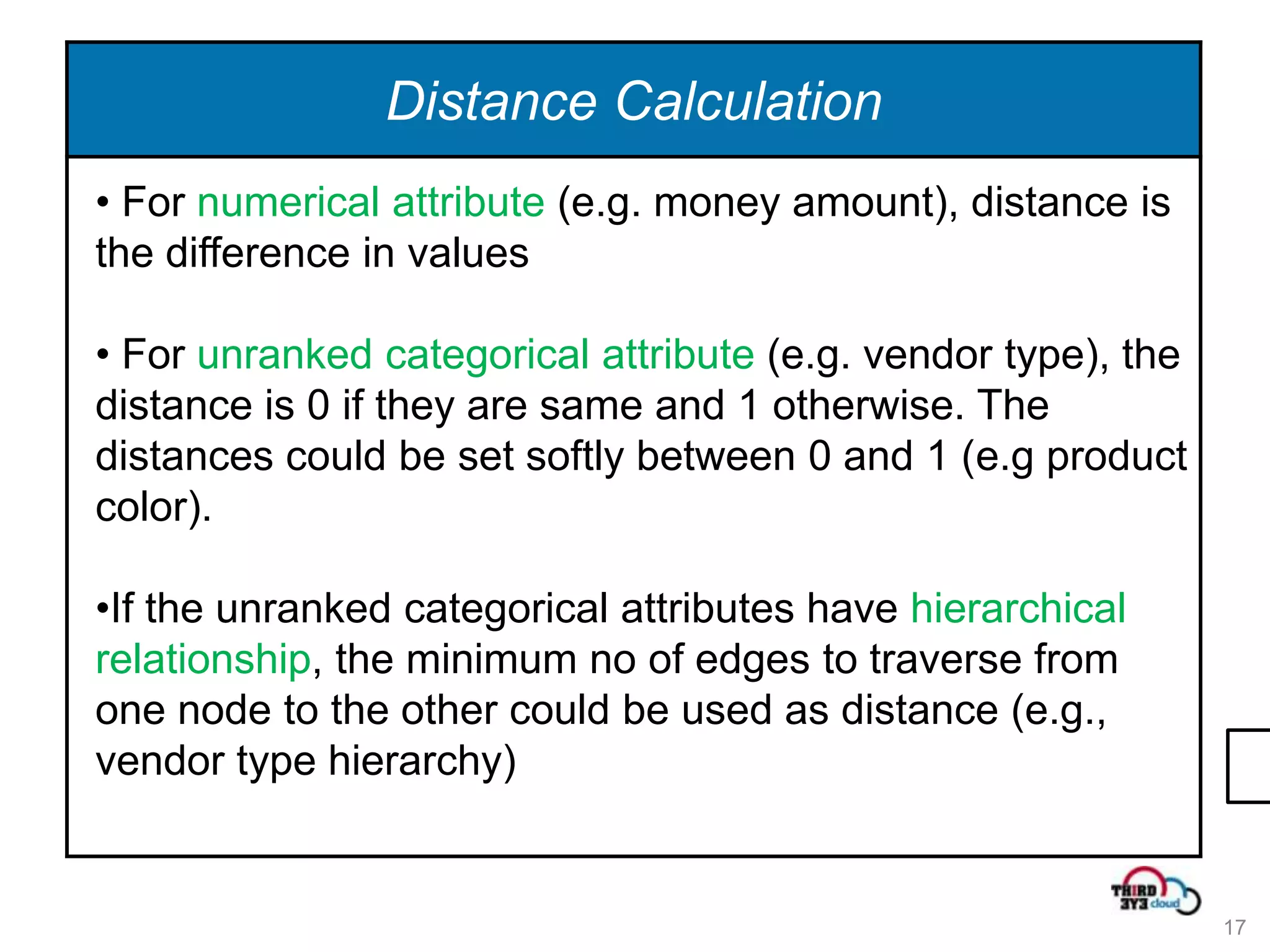
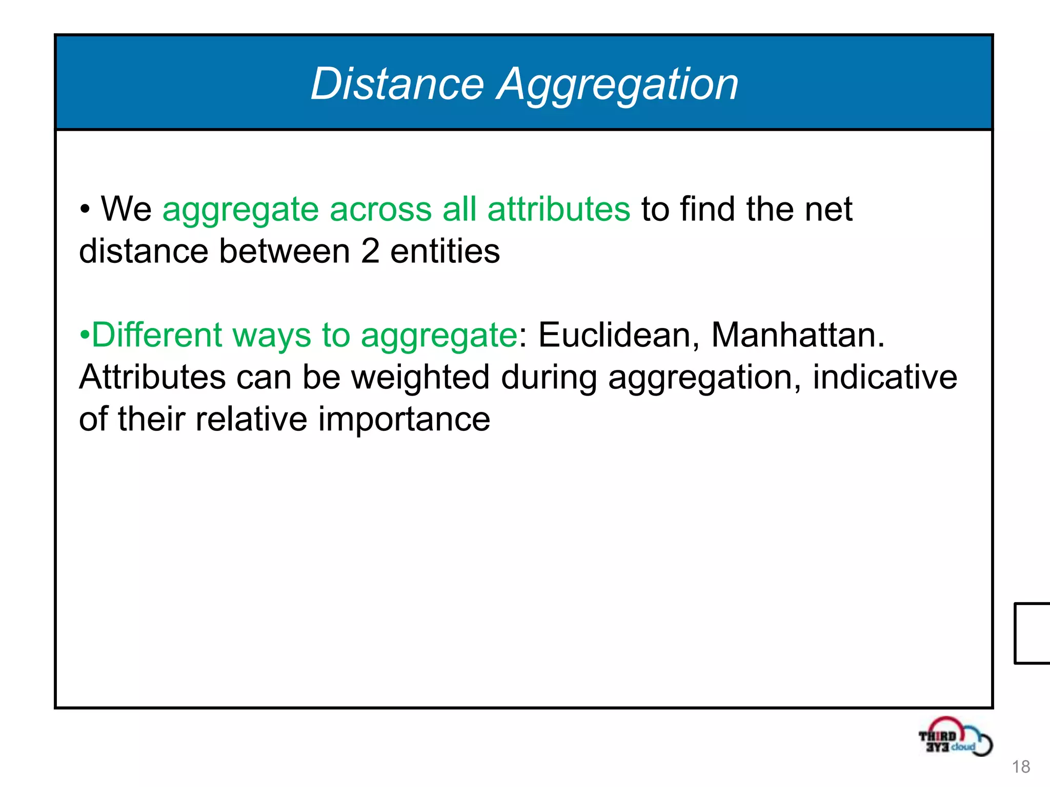
This document summarizes an expert talk on outlier and fraud detection using big data technologies. It discusses different techniques for detecting outliers in instance and sequence data, including proximity-based, density-based, and information theory approaches. It provides examples of using Hadoop and MapReduce to calculate pairwise distances between credit card transactions at scale and find the k nearest neighbors of each transaction to identify outliers. The talk uses credit card transactions as a sample dataset to demonstrate these techniques.


![Vibe Coding vs. Spec-Driven Development [Free Meetup]](https://cdn.slidesharecdn.com/ss_thumbnails/vibecodingvsspecdrivendevelopment-251209105622-43f455e7-thumbnail.jpg?width=640&height=640&fit=bounds)


