The document discusses curvilinear coordinates, specifically cylindrical and spherical polar coordinates, detailing their mathematical representations and derivatives. It emphasizes the utility of these coordinates in simplifying problems with symmetry in integrals, particularly those involving gradient, divergence, curl, Laplacian, and integrals. Additionally, the document explains the Dirac delta function and Helmholtz theorem regarding vector fields, addressing concepts of irrotational and solenoidal fields.

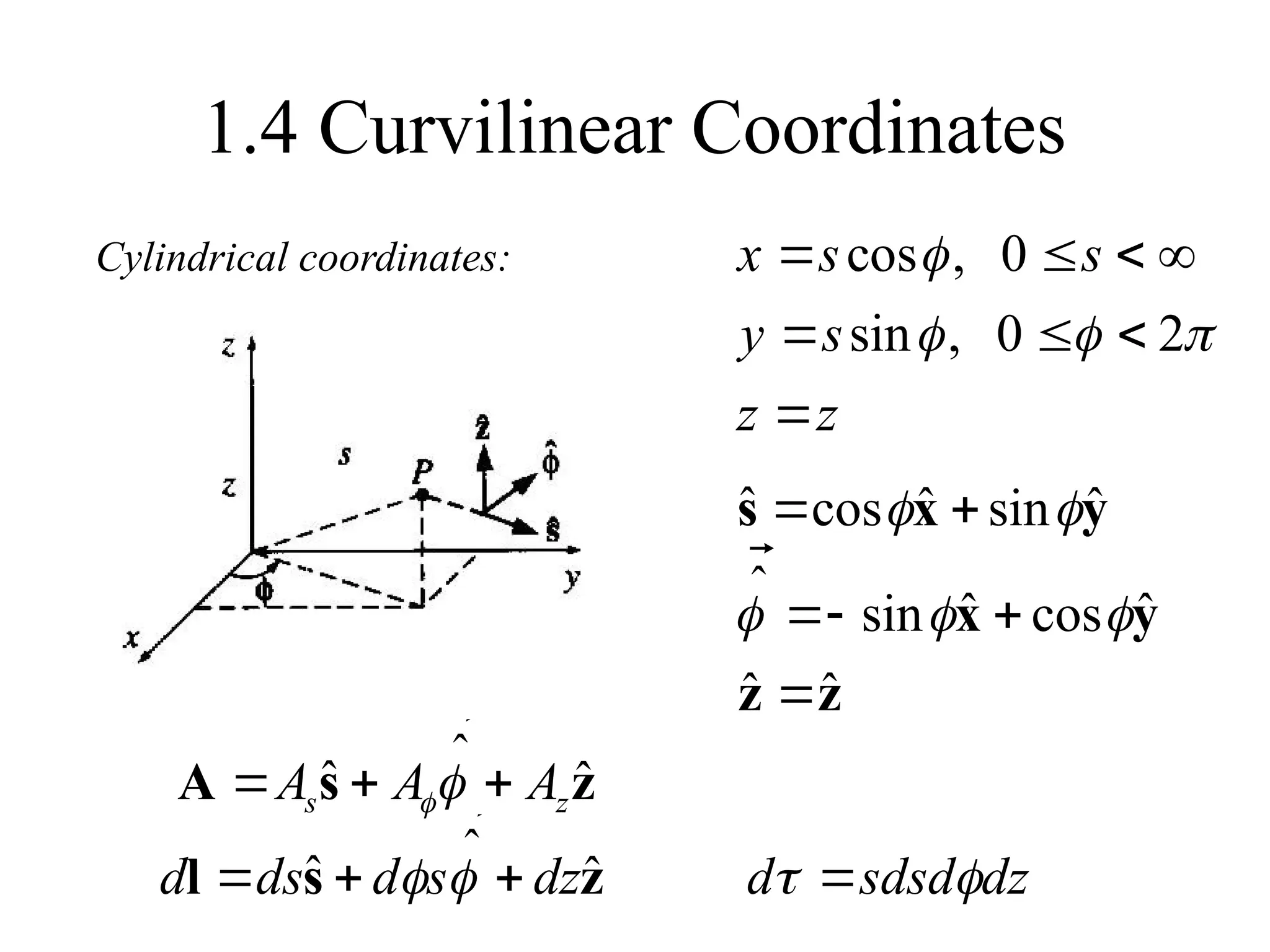
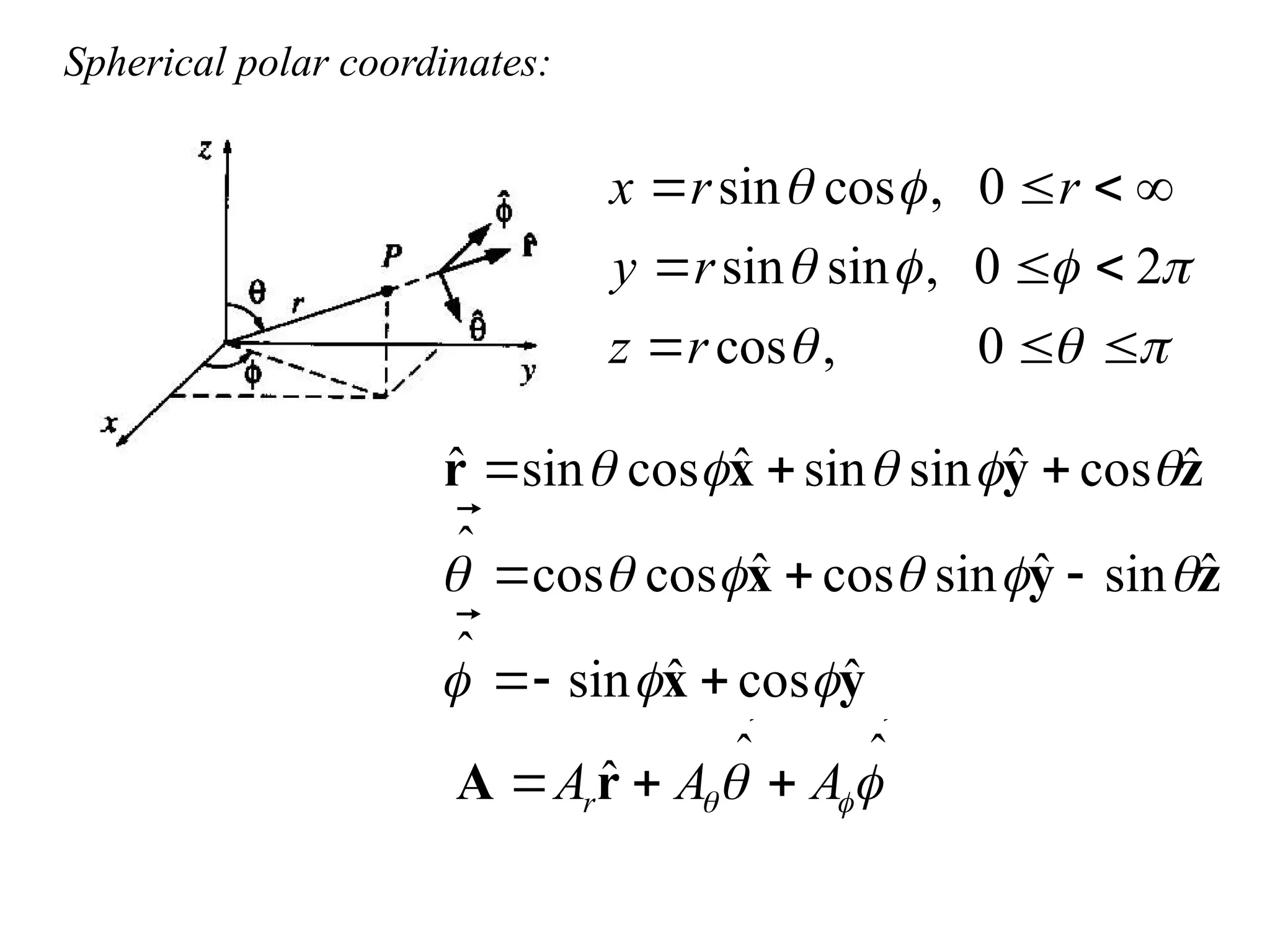
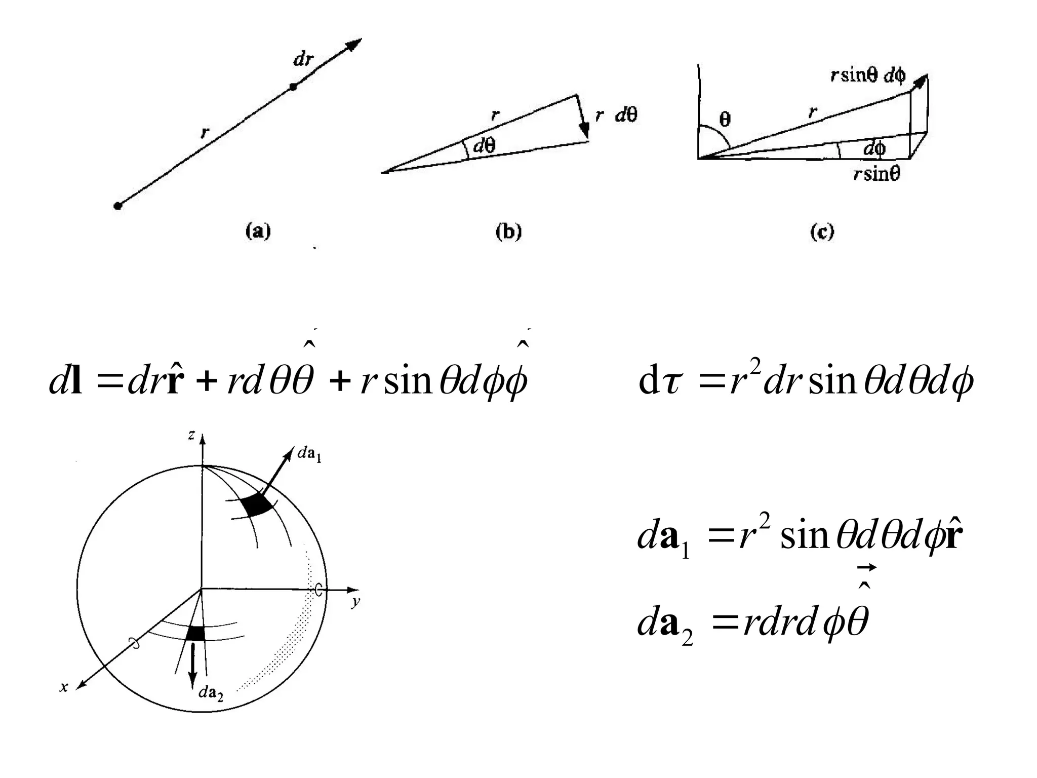
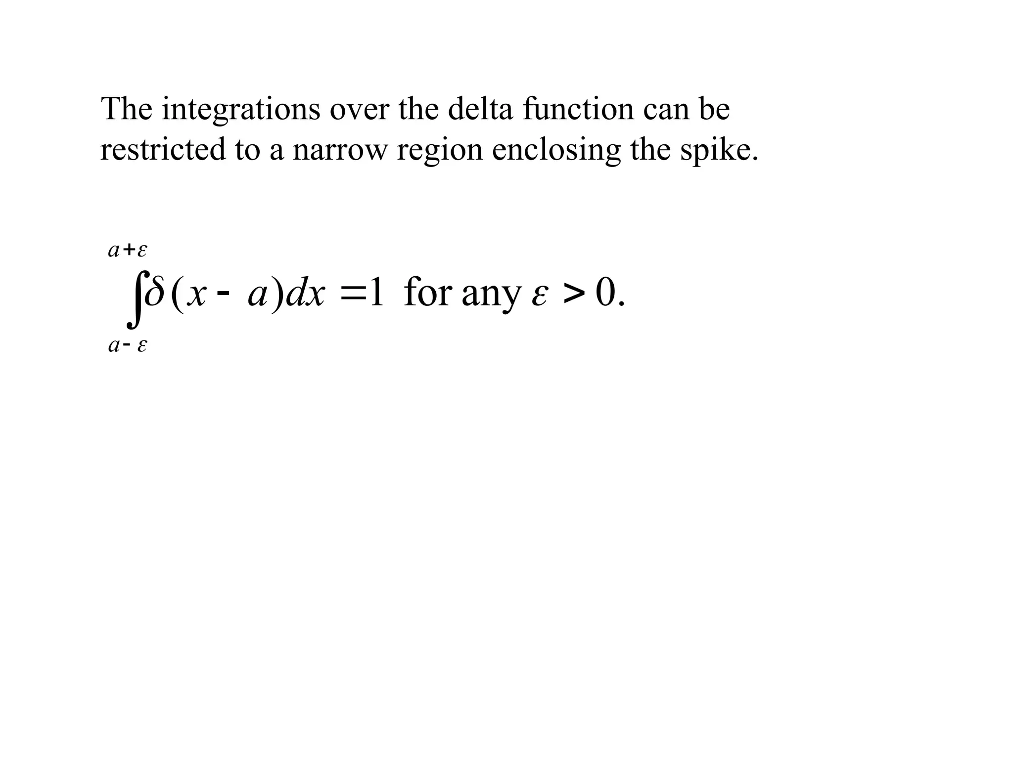
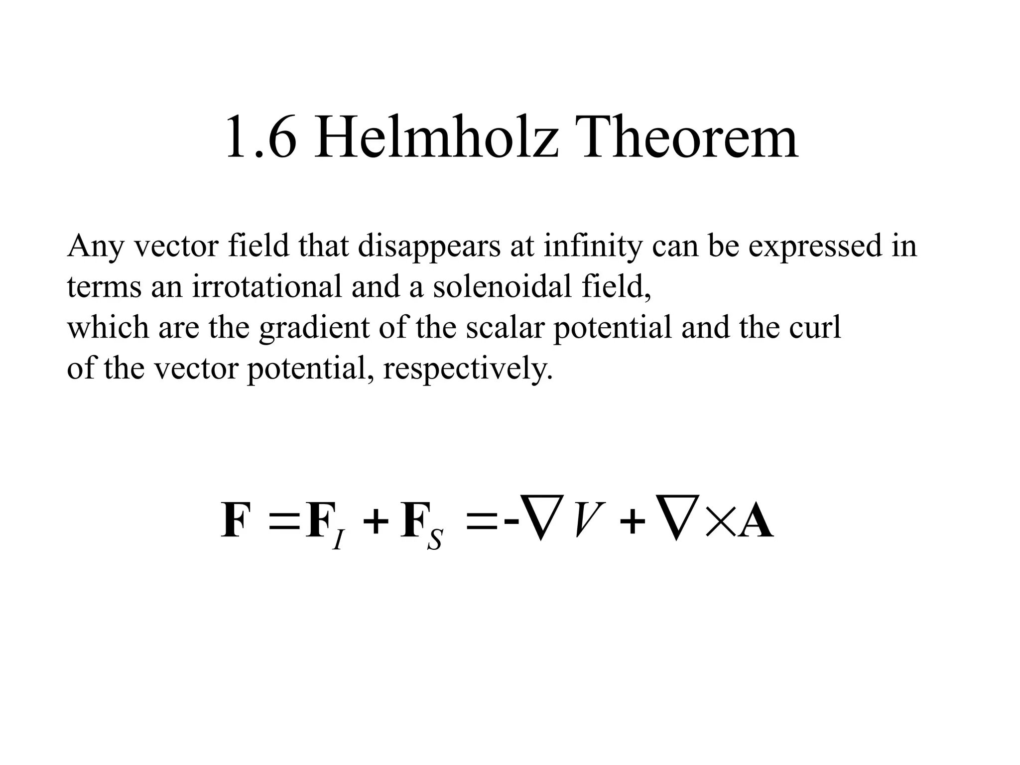
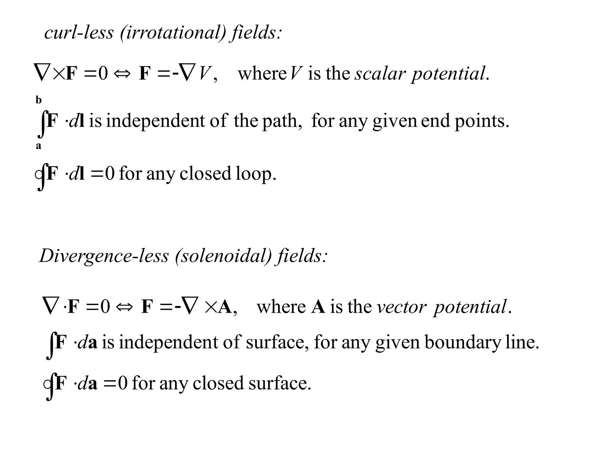
1. 1.4 Curvilinear Coordinates
Cylindrical coordinates:
dz
sdsd
d
dz
s
d
ds
d 


 


 ˆ
ˆ
ˆ z
s
l

z
z
s
y
s
s
x












2
0
,
sin
0
,
cos
z
z
y
x
y
x
s
ˆ
ˆ
ˆ
cos
ˆ
sin
ˆ
ˆ
sin
ˆ
cos
ˆ












z
s
A ˆ
ˆ
ˆ z
s A
A
A 

 



2. Spherical polar coordinates:



















0
,
cos
2
0
,
sin
sin
0
,
cos
sin
r
z
r
y
r
r
x
y
x
z
y
x
z
y
x
r
ˆ
cos
ˆ
sin
ˆ
ˆ
sin
ˆ
sin
cos
ˆ
cos
cos
ˆ
ˆ
cos
ˆ
sin
sin
ˆ
cos
sin
ˆ


























 

ˆ
ˆ
ˆ


A
A
Ar 

 r
A

3. 







 d
d
dr
r
d
r
rd
dr
d sin
d
ˆ
sin
ˆ
ˆ 2






r
l





ˆ
ˆ
sin
2
2
1

rdrd
d
d
d
r
d


a
r
a

4. Gradient, Divergence, Curl,
Laplacian, and Integrals
-Take into account the derivatives of the basis vectors.
-Working it out becomes often tedious.
-Find the results in the textbook.
-See Appendix for a compact form that generalizes to other
curvilinear coordinates.
-Expressions for the volume and surface elements in integrals
can be found in the Appendix.
For problems with spherical or cylindrical symmetry the
appropriate coordinates often lead to considerable
simplifications.

5. 3
r
r
v 

6. 1.5 The Dirac Delta Function











 1
)
(
and
0
0
0
)
( dx
x
x
if
x
if
x 






 )
0
(
)
(
)
(
)
(
)
0
(
)
(
)
( f
dx
x
x
f
x
f
x
x
f 








k
f
dx
kx
x
f
x
k
kx
)
0
(
)
(
)
(
)
(
1
)
( 


At the end, the delta function will appear under an integral.

7. Consider it as the limit of an infinite thin spike of area 1.
The shape of the spike does not matter.

8. three-dimensional delta function:



















space
all
space
all
f
d
f
dxdydz
z
y
x
d
z
y
x
)
(
)
(
)
(
1
)
(
)
(
)
(
)
(
)
(
)
(
)
(
)
(
3
3
3
a
a
r
r
r
r











)
(
4
)
1
(
)
(
4
)
ˆ
( 2
2
r
r
r

 




r
r

9. The integrations over the delta function can be
restricted to a narrow region enclosing the spike.
.
0
any
for
1
)
( 









a
a
dx
a
x

10. 1.6 Helmholz Theorem
Any vector field that disappears at infinity can be expressed in
terms an irrotational and a solenoidal field,
which are the gradient of the scalar potential and the curl
of the vector potential, respectively.
A
F
F
F 





 V
S
I

11. curl-less (irrotational) fields:
loop.
closed
any
for
0
points.
end
given
any
for
path,
the
of
t
independen
is
.
the
is
where
,
0











l
F
l
F
F
F
b
a
d
d
potential
scalar
V
V
Divergence-less (solenoidal) fields:
surface.
closed
any
for
0
line.
boundary
given
any
for
surface,
of
t
independen
is
.
the
is
where
,
0












a
F
a
F
A
A
F
F
d
d
potential
vector