IEEE CLOUD 2012 http://dl.acm.org/citation.cfm?id=2353798 Many business-oriented services will be gradually offered in the Cloud. Java Message Service (JMS) is a critical messaging technology in Java-based business applications, particularly to those that are based on the Java Enterprise Edition (Java EE) open standard. Maintaining high performance in the horizontally scaled, and elastic, cloud environment is critical to the success of the business applications. In this paper, we present practical considerations in optimizing JMS performance for the cloud deployment, where some of the findings may also serve to improve the design of JMS container so it adapts well to cloud computing. Our work also includes performance evaluation on the proposed strategies.

1. Optimizing JMS Performance for Cloud-based Application Servers
Zhenyun Zhuang ∗ and Yao-Min Chen ∗
∗ Oracle Corporation, 4180 Network Circle, Santa Clara, CA 95054, USA
Email: {zhenyun.zhuang,yaomin.chen}@oracle.com
Abstract—Many business-oriented services will be gradually
offered in the Cloud. Java Message Service (JMS) is a critical
messaging technology in Java-based business applications, par-
ticularly to those that are based on the Java Enterprise Edition
(Java EE) open standard. Maintaining high performance in
the horizontally scaled, and elastic, cloud environment is
critical to the success of the business applications. In this
paper, we present practical considerations in optimizing JMS
performance for the cloud deployment, where some of the
findings may also serve to improve the design of JMS container
so it adapts well to cloud computing. Our work also includes
performance evaluation on the proposed strategies.
Keywords-Cloud Computing; Application Server; JMS; We-
blogic Server; ZFSSA;
I. INTRODUCTION
Java Message Service (JMS) is a standard [1] for network-
based messaging, and a key example of Message-Oriented
Middleware [2]. It provides asynchronous transfer of mes-
sages and supports a queue-based as well as topic-based
communication model. The former facilitates one-to-one
communication while the latter, one-to-many. JMS is anal-
ogous to JDBC in that applications can use the same set
of APIs to communicate with each other. JMS is also an
important component in Java EE architecture, and it is
provided as both a service and a special type of enterprise
beans called message-driven bean (MDB). JMS addresses
the need of business applications that have evolved with
increased complexity and sophistication; it provides a mes-
saging service better in terms of scalability, reliability and
flexibility.
One of the emerging cloud-based service deployment is
Platform as a Service (PaaS), where customer applications
are deployed to platform servers that reside in the “cloud.”
One class of such platforms is Java EE-based application
servers [3] such as Oracle’s WebLogic Server (WLS) [4],
IBM’s WebSphere [5], and RedHat’s JBoss [6]. Brought
along with these application servers are the underlying
messaging services including JMS. In addition, through
messaging service infrastructure components such as Tibco’s
Rendezvous [7] and open-source ApacheMQ, JMS can
be used in cloud-based peer-to-peer (P2P), business-to-
business (B2B), and machine-to-machine (M2M) applica-
tions. Furthermore, JMS sees a natural fit into the service-
oriented architecture (SOA), which enables loosely-coupled
and protocol-independent components to interact with each
other. In particular, a recent advancement of SOAP [8] is
that JMS is considered to be the carrying protocol for SOAP
services [9].
For moving into the cloud, a messaging service typically
needs to meet the reliability, scalability, elasticity and per-
formance requirements of the cloud deployment. This paper
addresses the performance requirement and in particular, we
address the performance of JMS as part of an application
server (AS). In other words, the AS is the hosting container
of the JMS component. Although an AS can be implemented
with different technologies, Java EE-based implementation is
popular, mainly due to its standard-based approach where an
application (known as “servlet”) can be deployed to different
AS implementations.
Within the AS context, JMS can be configured to be in
either persistent mode or non-persistent mode. The former
means that the AS keeps an non-volatile copy of the mes-
sages that it receives, so the messages are not lost when
the AS crashes or restarts. By contrast, in the non-persistent
mode the messages are only kept in the system memory.
When reliability is necessary, as needed by mission-critical
applications, the persistent mode is preferred. So in this
paper we study using a ZFS [10] based network-attached
storage appliance [11] to persist the JMS messages. The
appliance is connected to the AS via InfiniBand [12] for
high bandwidth and low latency.
Based on the aforementioned setup, our investigation
leads to three key performance improvement strategies. They
are: (i) matching storage block size with message size,
(ii) applying distributed persistent stores, and (iii) choosing
appropriate storage profiles. And our contributions can be
summarized as: (i) We investigated the problem of optimiz-
ing JMS performance and highlighted a typical deployment
with Weblogic and ZFS storage appliance (ZFSSA); (ii) We
proposed a set of performance improvement strategies; and
(iii) We evaluated the resulting JMS performance based on
the strategies.
For the remainder of the paper, we first provide back-
ground information and highlight the problem definition in
Section II. We then present the detailed strategies in Section
III. We perform performance evaluation and show the results
in Section IV. We also present related works in Section V.
And finally in Section VI we conclude the work and list our
future activities.
2012 IEEE Fifth International Conference on Cloud Computing
978-0-7695-4755-8/12 $26.00 © 2012 IEEE
DOI 10.1109/CLOUD.2012.136
828
2012 IEEE Fifth International Conference on Cloud Computing
978-0-7695-4755-8/12 $26.00 © 2012 IEEE
DOI 10.1109/CLOUD.2012.136
828

2. WebLogic
Server
Application
Server (e.g.,
WebLogic)
ZFSSA
Storage
Storage
(e.g., ZFSSA)
Internet
InfiniBand
Ethernet
JMS clientEE backend
JMS clients
Infiniband
Ethernet
JMS clientEE backend
Internet
JMS clientDesktop JMSJMS clientMobile JMS
Internet
JMS clientEE backend
JMS clients
JMS clientDesktop JMS
clients
JMS clientMobile JMS
clients
Figure 1. Cloud-ready JMS system
II. BACKGROUND AND MOTIVATION
In this section, we first provide background information
regarding JMS and WLS. We then highlight the importance
of investigating their performance and explain the choice
of JMS implementation in WLS. We finally present the
definition of the problem studied in this work.
A. Background
1) JMS: It is one of the mostly used middleware com-
ponents in Java EE architecture. JSR 914 [13] defines
an API for accessing enterprise messaging systems from
Java programs. It dictates how the programs send messages
from one application to another, potentially exploiting a
transactional quality of service (QoS). The messages can
be of several types including byte, text or object-based. JMS
also supports two modes of message delivery: Point-to-Point
(PTP) and Publish and Subscribe (Pub/Sub). The former
is also known as queue-based message delivery, while the
latter, topic-based.
2) Application Server (AS) and WebLogic Server (WLS):
An AS can be implemented with either Java EE, .NET, or
PHP frameworks. Commercial AS such as WLS and Web-
Sphere use Java EE framework. WLS is a key middleware
product from Oracle. which includes the following key com-
ponents: HTTP web server, messaging service, enterprise
portal and Tuxedo, etc. WLS is widely used, supports rich
set of features, and is the foundation for Oracle Fusion
Middleware [14]. Hence it is the AS used for this study.1
Note that, since WLS is based on the Java EE standard, it
is quite likely that some, if not all, of the findings in this
paper can be applicable to other application servers.
3) Cloud Computing: With the premise of better eco-
nomic efficiency and performance scalability, cloud com-
puting has attracted much attention from both the research
1The WLS version used for this study is 10.3.6 (a.k.a., 11g Release 1),
which was released in September 2011.
community and the industry. It provides elastic (or resiz-
able) compute capability. Amazon EC2 [15], for instance,
allows customers to dynamically allocate and de-allocate
compute resources to accommodate customers’ computing
requirement. Cloud Computing best fits computing jobs that
have bursty requirement. By leveraging cloud computing, a
service provider can better adapt to the changing needs for
better performance and reduced cost. Before the mission-
critical business applications can be deployed into the cloud,
we would like to first make sure that the critical middleware
components such as messaging service can work well in the
cloud, which motivates our study of JMS in the cloud.
4) JMS in the Cloud: Recently Amazon has built a cloud-
based messaging system [16] that is sematically similar to
JMS. The trend is followed by other deployment cases [17].
Even though the exact JMS cloud deployment model is still
evolving, for a particular business that requires JMS-based
applications, we will likely see the following three deploy-
ment scenarios based on typical business usages. (i) Full
Cloud Deployment. The application servers are all deployed
in cloud and used exclusively for cloud-based applications.
(ii) Partital Cloud Deployment. A portion of application
servers are deployed in the cloud to serve some cloud-ready
applications, while the rest of application servers are still
deployed locally for the remaining applications, which are
kept within the enterprise perimeter because of application
limitation or security constraints. (iii) Hybrid Cloud Deploy-
ment. Workload is handled with local application servers
in low-load scenarios, while extending to cloud-deployed
application servers when the load becomes high. Such a
deployment model exploits the elastic nature of the cloud, in
the sense that cloud-based servers complement local servers
when necessary. Note that in all scenarios, it is expected
that high performance network links are used to connect the
application servers.
829829

3. B. Problem Definition
The problem context that we will study is as follows. The
assumption is that JMS works in a particular cloud pro-
duction deployment. Such a deployment scenario includes
the following components, as shown in Figure 1: (i) One
or multiple JMS server nodes (e.g. WLS) serving as JMS
providers; (ii) One or multiple JMS client nodes that are
connected to the server nodes with either InfiniBand or
through Internet, where these JMS clients can be other
Java EE backend servers, mobile clients or desktop clients;
and (iii) One or multiple network-attached storage (NAS)
appliances (e.g., ZFSSAs). Note that the third component of
storage appliances is used for JMS persistent mode. With
the above assumptions, the problem comes down to the
following. Given such an environment, how can we optimize
the JMS performance as experienced by the JMS clients?
Please note that we do not just study the application
servers in isolation. We also study the underlying network
IO and storage (ZFSSA) optimizations needed to achieve
best efficiency. From the study we develop a set of three
deployment strategies to optimize the JMS performance.
They span across the AS layer, the network layer and the
storage layer. They will be explained in the next section.
III. OPTIMIZATION STRATEGIES
With the problem defined in Section II, we now elabo-
rate on the strategies that help improve JMS performance
in cloud. The strategies are as follows. In the AS layer,
one should try matching the storage block size with JMS
message size profile. In the networking layer, one should try
applying Distributed Persistent Stores. And in the storage
layer, we should choose appropriate Storage Profiles. Our
description refers to a typical setup to be depicted in detail
in Section IV-A. The setup consists of a JMS “producer” to
send messages to WLS and a JMS “consumer” to receive
the messages. In a cloud setting, the JMS producer and
consumer each can be an application residing in a virtual
machine deployed in a data center.
A. Applying Distributed Persistent Stores
To explore parallel processing, WLS is able to simulta-
neously use multiple persistent stores (e.g., multiple files).
This is achieved by configuring multiple JMS destinations,
each with a separate persistency store. Use of distributed
persistent stores is coupled with using UDDs (Uniform
Distributed Destinations), where multiple JMS destinations
are grouped together into a single sub-deployment. Unlike
standalone queue and topic resources that can only be
targeted to a specific JMS server in a domain, UDDs can
be targeted to multiple JMS servers, WLS instances, or to
a cluster. There are two types of UDDs. They are UDQs
(Uniform Distributed Queues) for queue-based JMS, and
UDTs (Uniform Distributed Topics) for topic-based JMS.
By using distributed destinations, WLS is able to spread
and balance the IO workload across multiple destinations,
which can gain benefits including fail over, better use of
resources, improved response times and increased through-
put. WLS supports two different algorithms for balancing
the workload across the destinations: Round-Robin Distri-
bution and Random Distribution. The round-robin algorithm
maintains an ordering of the defined destinations within the
distributed destination. New messages are then distributed
to the next destination according the the defined ordering
in the configuration file of config.xml. Random distribution
algorithm, however, supports weighting. It uses the weights
assigned to the physical destinations to dispatch the mes-
sages.
1) Impact of Distributed Stores: Multiple persistent
stores, used separately by different UDD destinations, can
be used to achieve parallelism. The persistent stores can be
a server instance’s default store, a user-defined file store,
or a user-defined JDBC-accessible store. Using distributed
persistent stores helps alleviate storage IO bottleneck. For
instance, if a single storage appliance (e.g., ZFSSA) has
reached its IO limit, then using multiple appliances con-
currently can improve the throughput by removing the IO
bottleneck. For ease of explanation, subsequently we will
only use UDQs to elaborate the benefits of distributed stores.
The discussion for UDTs, while omitted, should be similar.
2) Uniform Distributed Queues: In the case of UDQs,
different queues in UDQs are balanced by WLS, and
incoming messages are distributed into the queues. The
load balancing algorithm affects both JMS producers and
consumers, but in different ways. On the producer side, for
each message sent, WLS will determine the destination for
the incoming message according to the balancing algorithm.
On the other hand, for a consumer, the balancing decision
is made only once. When a consumer is created, WLS will
determine the destination bound to that consumer. From then
on, the consumer always receives messages from the pre-
determined destination.
When applying distributed persistent stores, one has to
consider multiple factors including application requirements,
number of JMS consumers, and reliability requirement. First,
applying multiple persistent stores particularly help in the
scenarios where persistent storage tends to be the JMS
performance bottleneck. Second, since the JMS consumers
are statically assigned to a distributed JMS destination, the
UDQ set size should not exceed the the consumer set size.
Third, the number of UDQs has to be at least the number
of storage devices since each JMS server can only link
to one persistent store. Note that each storage device can
correspond to multiple persistent stores, since multiple store
files can reside on the same device.
Configurations of UDQs and persistency can be done
by changing the JMS system modules (i.e., either directly
changing the configuration file or from the web console)
830830

4. and creating sub-deployment inside the system module. The
sub-deployment groups the multiple queues together with a
single JNDI name.
B. Choosing Appropriate Storage Profiles
Cloud storage devices often feature RAID (redundant
array of independent disks) configurations that combine mul-
tiple disk drive components into a logical unit. Depending
on the RAID levels configured, storage devices can provide
a balance among capacity, reliability and performance. For
instance, RAID-1 provides simple mirroring among disks
with highest reliability but lowest capacity, while RAID-0
can achieve the highest capacity, but with lowest reliability.
In addition, different RAID levels, along with read/write
caching mechanisms available on the storage devices, often
result in different performance with respect to read and
write operations. For instance, mirroring (e.g., RAID-1)
typically has better read performance than write. We refer
to the relevant configuration of storage devices as “storage
profiles”.
1) Impact of Storage Profiles: ZFS storage appliances,
which are based on ZFS file system [10], are enterprise-
level options for JMS persistency storages. They support
several “data profiles” which define how the storage disks are
organized to balance among performance, capacity and re-
liability. ZFSSA 7320, for instance, supports 6 data profiles
including Double Parity RAID, Mirrored, Striped, and Triple
mirrored. Among them the Mirrored data profile provides the
highest reliability, but reduces the capacity by two thrids.
By comparison, Striped data profile leads to the maximum
capacity, but supports no redundancy.
Besides the data profile, there are also a log profile and
a cache profile that need to be configured. Particularly, the
log profile specifies how the ZFS internal flash-based log
devices (i.e., Logzillas) are configured. For certain write
operations, data is written to Logzilla and the operation
can be acknowledged to the client instantly. So rather than
acknowledging in the order of milliseconds due to disk
latency, Logzilla responds in about 100us. Log profile has
two types: mirrored and striped, and striped log profile tends
to expedite the writing rate at the expense of reliability.
In Table I, we show the IO rates of six data profiles and the
resulting storage capacities for a particular NFS mounting
Data Profile Capacity Raw IO rate
Double Parity 1.58 0.99
Mirrored 1 (base) 1 (base)
Single Parity 2.11 0.99
Striped 2.12 1.09
Triple Mirrored 0.63 1.00
Triple Parity 1.84 0.95
Table I
IMPACT OF STORAGE PROFILES (THE RESULTS ARE NORMALIZED WITH
RESPECT TO THE DEFAULT CONFIGURATION OF MIRRORED PROFILE)
setup with a ZFSSA. For all profiles, the cache and log
profiles use the default setting (i.e., mirrored). The results
are obtained by running 4 simultaneous writing processes.
Each writing process corresponds to a “dd” command that
continuously writes data to the ZFSSA. We can see that
depending on the data profile, the raw IO rate and capacity
vary.
2) Application-specific Configuration: When determining
the appropriate data profile for JMS applications to use, one
has to assess the JMS persistency requirement for the partic-
ular applications. If maximum reliability is preferred, then
high-reliability data profiles such as Mirrored and Double
Parity profiles should be used. However, if throughput is of
higher priority, or ZFSSA reliability is maintained through
appliance clustering, then using striped data profile could
improve the JMS throughput. In addition, striped data profile
also has the highest capacity. Note that it is also possible to
find a balance between reliability and performance by using
other profiles.
For maximum JMS throughput, full striping can be used
so that data can be parallelly processed. Note that depending
on specific usage environments, full striping does not nec-
essarily lead to compromised reliability. If the applications
are not sensitive to reliability, or the deployment has other
reliability features enabled (e.g., hot-standby servers), then
increasing striping might be a reasonable approach towards
maximized JMS performance. Since this is usage-specific,
we will not delve deeper into the discussion regarding when
to use full striping.
3) Changing Storage Profiles: When changing storage
profiles, one has to consider the deployment setup, applica-
tion requirements, and the performance tradeoffs regarding
reliability, capacity and IO rate. First, if the storage devices
are only used for the WLS applications, then it might make
sense to focus more on the reliability and IO rate, but less
on capacity, as today’s high-end storage devices typically
have far more capacity than regular WLS applications need.
Second, if applications themselves are designed to tolerate
JMS message losses, then storage reliability should be of
less concerns. Third, in typical WLS running environments,
JMS applications tend to write considerably to the storages,
thus the deployment should apply a data profile that has
better writing performance. Fourth, as we will demonstrate
in Section IV, using striped log profile results in higher JMS
throughput and thus helps in scenarios where throughput has
a higher priority.
Most storage appliances, including ZFSSA 7320, provide
BUI (Browser User Interface) to users for administration and
monitoring purposes. The configuration of storage striping
can be done conveniently in this manner. Alternatively, these
storage appliances may also provide CLI (Command Line
Interface) to performance various tasks including storage
configurations.
831831

5. 0.99
0.995
1
1.005
1.01
1.015
1.02
1.025
1.03
0 2000 4000 6000 8000 10000
Block Size (Byte)
Throughput
(a) JMS Throughput
0.8
0.9
1
1.1
1.2
1.3
1.4
0 2000 4000 6000 8000 10000
Block Size (Byte)
IO Rate
(b) Storage IO rate
Figure 2. Impact of Block Size (message size is 500 bytes and the results are normalized with respect to the default block size of 512 bytes)
C. Matching Block Size with Message Size
In persistent mode, JMS messages are stored by WLS in
a non-volatile storage for the purpose of reliability. In WLS,
each message is represented by and stored in one or more
“blocks”. Note that here the block is a fixed consecutive
bytes of memory intrinsic to WLS, not to be confused with
a file block, the storage unit used by the storage device
or server. The block size is one of the user-configurable
parameters in WLS, and its configuration affects the required
storage space and bandwidth capacity. While the storage can
be either a local file system, storage-area network (SAN) or
network-attached storage (NAS). We envision that NAS will
be commonly used in cloud deployment, and choose it to
be the subject of study in this paper. In particular, we study
ZFSSA, which is a type of NAS. For our study, we attach
one or more ZFSSAs to WLS for the purpose of persistent
storage.
1) Impact of Block Size: The blocks are WLS units for
writing to and reading from the storage. Here we show, by
an example, that the block size parameter affects both JMS
throughput and storage IO rate. In Figure 2(a), we show the
experiment results of JMS throughput by having the JMS
producer to send fixed sized messages to WLS and the JMS
consumer to receive the messages via the WLS. The JMS
message size is fixed at 500 bytes.2 We vary the block sizes.3
As block size varies, the JMS throughput changes as well.
It achieves the highest throughput when the block size is set
at 2048 bytes. We also show the corresponding storage IO
rate in Figure 2(b).
The block size is a parameter that can be configured by
the user. Since it is desirable to have higher JMS throughput
in most deployment scenarios, it is necessary to configure
the appropriate block size so that JMS throughput can be
maximized. In production deployment scenarios, the JMS
message sizes used by the particular application may not
vary wildly. Thus, by understanding the relationship between
2For ease of presentation, we only mention the size of the message body,
but an actual JMS message is stored along with other components such as
headers and properties.
3The block size parameter for WLS needs to be a power of 2, between
512 and 8192 bytes.
the message sizes and the block size, it is possible to set a
“sweet” value for block size so that the JMS performance
is maximized for a deployment environment.
2) Message Profiling and Block Size Configuration:
Since block size is one of the tunable parameters of WLS,
in real deployment scenarios, if the JMS message sizes
of the applications are known, then an appropriate block
size can be set. If the JMS message sizes are unknown,
then customers could perform message size profiling to
learn the message sizes used by the particular applications,
then accordingly set appropriate block sizes to maximize
JMS performance. Specifically, by running WLS that with
different block sizes and comparing the JMS performance,
an optimal block size can be determined.
As we have observed that there is an intricate interplay
between the block size and message size, it is worthwhile
to profile the message size distribution of an application in
order to achieve best JMS persistent mode efficiency. The
message size information can be obtained in several ways.
First, if the application design is known, it is possible to
accordingly get such information. Second, for a running ap-
plication, the WLS Admin Console’s monitoring service can
see the message properties including the sizes, where some
post processing can extract the message size distribution.
Third, it is also possible to perform network level sniffing
to obtain the message size information.
In some usage scenarios, the block size might not be
convenient to change. For instance, if a JMS provider has
been used by other applications, and when a new application
is designed or deployed, it may be better to have the new
applications adapt and fit with the existing block size. More
precisely, if the new application has flexibility in setting its
JMS message size, we may adjust it to fit better with the
existing WLS block size.
IV. EVALUATION
In this section, we provide experimental results for the
proposed deployment strategies. We will first describe the
testbed setup, which will then be followed by results specific
to each strategy.
832832

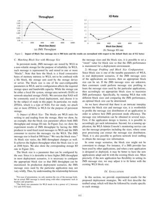
6. 0
0.5
1
1.5
2
2.5
3
-1 1 3 5 7 9 11 13
Number of UDQs
Throughput
(a) JMS Throughput
0
0.2
0.4
0.6
0.8
1
1.2
-1 1 3 5 7 9 11 13
Number of UDQs
Receiver Response Time
(b) Receiver Response Time
Figure 3. Impact of UDQs (the results are normalized with respect to the case of one queue)
A. Testbed Setup
The testbed was set up with the following hardware, OS,
JVM (Java Virtual Machine) and WLS configurations.
1) Hardware and OS: The server hosting WLS is an
Oracle SPARC T4-2 server with 128GB memory. It has dual
SPARC T4 processors with combined 128 hardware strands
that run at 2848 MHz. The server is installed with Solaris
11 and configured with two Logical Domains (LDoms) each
with 64 strands. We run a WLS instance in one of the
domains.
2) ZFSSA: The storage appliance is a Sun Storage 7320
(40 disks with 21.5TB capacity). It is connected to the server
through 40Gbps InifiniBand, running the IP over IB (IPoIB)
upper layer protocol. The ZFSSA is exposed to the server
as an NFS network drive.
3) WLS: The WLS instance operates in Production mode,
and is configured to work with both a single queue and
UDQs. Other important configurations include: Scattere-
dReadsEnabled=true, GatheredWritesEnabled=true, thread-
pool.MaxPoolSize=30, SocketReaders=20. The WLS ver-
sion is version 10.3.6, 2011 Oct 30, 1437254.
4) Java: The JVM used is HotSpot 1.7. The important
options configured for the JVM are: -Xms16g, -Xmx 16g,
-Xmn6g, -XX:ParallelGCThreads=8.
5) Benchmark: Our benchmark uses Faban [18] as har-
ness. Faban is an Oracle-developed benchmark harness and
driver development framework, which has been used in
SPECjEnterprise2010 [19] and SPECsip Infrastructure2011
[20] benchmarks. We develop our workload driver under
the Faban driver framework. The benchmark drives a JMS
producer and a JMS consumer, which are carefully chosen to
avoid being performance bottleneck. The driver machines are
connected to the server, through InfiniBand running IPoIB.
The JMS messages are produced and consumed in a non-
transactional mode. Unless otherwise specified, the messages
are of the “byte” type and have 8k-byte message body.
B. Distributed Persistent Stores
First, we evaluate the impact of using UDQs in persistent
mode. We use a single ZFSSA with Striped data profile,
and set the block size to be 512 bytes. The number of
queues vary from 1 to 9. The performance results are
shown in Figure 3. As Figure 3(a) shows, JMS throughput
increases with the number of queues. The improvement is
more significant when the number of UDQs is relatively
low, compared with the incremental improvement when the
number is high. In Figure 3(b), it shows the response time
becomes lower with the increase in the number of queues.
Similar to the throughput curve, the response time curve has
a knee point where the improvement becomes incremental.
C. Storage Profiles
The storage profile configuration with ZFSSA 7320 con-
sists of three parts: data profile, log profile and cache
profile. Depending on the hardware availability, the three
types of profiles allow users to configure the disks, logging
devices and caching devices for balancing among multiple
performance metrics. The effect of configuring data profile
has been shown in Table I. While different data profiles lead
to different total capacities and different levels of reliability,
the throughput numbers do not seem to differ significantly.
In fact, in our experiment, we have found that log profile is
a more direct factor that affects the JMS throughput.
We also measure the effect of log profile on the JMS
throughput and receiver response time. We compared the
performance results for two types of log profiles: mirrored
log and striped log, where we set the block size to 512 bytes,
and used one ZFSSA and nine queues. With the striped
log, JMS throughput is 11% higher than mirrored log and
response time is 11% lower.
D. Storage Block Size
We now evaluate the impact of setting block size. We use
nine queues with a single ZFSSA.
1) Optimal block size for a given message size: Here we
try to identify the optimal block size, assuming we have
a fixed message size. We iterate through different message
sizes from 500 bytes to 4000 bytes. For a given message size,
we iterate through different JMS block sizes (as allowed
by WLS). We first notice that the storage IO sizes differ
quite a lot when we vary the block sizes for fixed message
sizes. In terms of JMS throughput, for several message
sizes, the throughput numbers within the row do not differ
833833

7. 0.98
0.985
0.99
0.995
1
1.005
1.01
1.015
1.02
1.025
0 2000 4000 6000 8000 10000
Block Size (Byte)
Throughput
(a) JMS Throughput
0.975
0.98
0.985
0.99
0.995
1
1.005
1.01
1.015
1.02
1.025
0 2000 4000 6000 8000 10000
Receiver Response Time
(b) Receiver Response Time
Figure 4. Throughput under different block sizes (where messages have
a random size between 1KB and 2KB, and the results are normalized
with respect to the default block size of 512 bytes)
much; but for some message sizes, such as 4000 bytes,
the throughput number can differ significantly. In Table II,
the JMS throughput numbers for a particular message size
and different block sizes are shown in rows. The reasons
why JMS throughput does not change much for certain
message sizes are that the IO storage is not the performance
bottleneck.
2) Optimal block size for a given message size distribu-
tion: We also consider a scenario where the messages are of
different sizes. Assuming a uniform distribution of message
sizes between 1000 bytes and 2000 bytes, we generate JMS
messages with size randomly chosen in the interval. We then
measure the JMS performance for all valid block sizes. The
results are shown in Figure 4. From the results, we see that
Msg Size Blk=512 1024 2048 4096 8192
500 1 1.01 1.03 1.01 1.01
1,000 1 0.99 1.04 1.03 1.02
1,500 1 1.03 1.04 1.03 1.02
2,000 1 0.97 0.93 0.93 1.02
2,500 1 1.00 0.93 0.94 1.03
3,000 1 0.95 0.98 0.97 0.97
3,500 1 1.01 1.00 0.98 0.99
4,000 1 0.98 0.90 0.75 0.77
Table II
FINDING THE OPTIMAL BLOCK SIZE (JMS THROUGHPUTS ARE
NORMALIZED WITH RESPECT TO THE BLOCK SIZE OF 512 BYTES)
0
5
10
15
20
25
30
35
40
45
0 1000 2000 3000 4000 5000 6000 7000 8000 9000
Message Size (Byte)
JMS Traffic Rate
Figure 5. Finding the optimal message size (results are normalized
with respect to message size being 100 bytes)
the optimal block size that yields to highest JMS throughput
is 8192 bytes and the corresponding response time is also
the lowest.
3) Applications adaptation to fit a block size: If block
size is known or fixed in an environment, one may adjust
message sizes of a JMS application to fit the predetermined
block size to achieve optimal JMS throughput. Such adjust-
ment can occur in two ways. First, if the application is being
developed, then the message sizes used by the applications
can be set to the optimal values. Second, the adjustment can
also be done when the application has been developed and
it allows users to change the message sizes. We considered
a scenario where block size is set to 8192 bytes. We then
varies the message size from 100 bytes to 8500 bytes, and
measure the JMS throughput. Since the message sizes differ,
we use bytes per second as the throughput metric. The results
are shown in Figure 5. We see that when the messages are
7500-byte long, the JMS throughput peaks.
V. RELATED WORK
In this section we survey the related literature and draw
the relationship between our work and others.
A. Workload Characterization for Application Servers
There have been research efforts attempting to charac-
terize the workload for driving various types of application
servers [21]–[23]. Some of the works focus on commercial
application servers such as WLS [23], while others target
open-source application servers. Our work specifically char-
acterizes the JMS workload on WLS.
B. JMS and AS Performance Analysis
There have been earlier studies on JMS performance
[24]–[28]. Menth and Henjes [27] analyzed the message
waiting time with a FioranoMQ JMS Server. Henjes el al
[24] studied the filtering performance of three JMS servers
FioranoMQ, SunMQ and WebsphereMQ, and subsequently a
SunMQ-focused study [25] provided a model for describing
the service time. Our work distinguishes in that we study
WLS, its JMS persistent mode, and the deployment with
ZFSSA in the cloud.
834834

8. C. Industry Best Practices
It is quite a common industry practice to provide rules of
thumbs for maximizing application performance, e.g., [29],
[30]. Most of these efforts are specific to certain products,
while others are more generic and can apply to a large range
of industry products. The strategies provided in this paper
can be taken as best practices for running JMS on WLS.
VI. CONCLUSION
In this work, we study the problem of deploying JMS
in the cloud. Working with a particular JMS setup, we in-
vestigate three strategies for maximizing JMS performance.
We then provide empirical data from testing a real product
to evaluate the strategies. It is advised that one should
analyze his or her application need (e.g., reliability versus
performance), perform JMS related message profiling, and
configure WLS accordingly to achieve optimal performance.
Note that there are a variety of other tuning strategies [31]
that should be considered as well.
REFERENCES
[1] Java Message Service (JMS) API,
http://jcp.org/en/jsr/detail?id=914.
[2] E. Curry, “Message-oriented middleware,” in Middleware for
Communications. Chichester, England: John Wiley and Sons,
2004.
[3] Application Server, http://en.wikipedia.org/wiki/Application server.
[4] Oracle WebLogic Server, http://www.oracle.com/technetwork/
middleware/weblogic.
[5] WebSphere Software, http://www-
01.ibm.com/software/websphere.
[6] JBoss Enterprise Middleware,
http://www.redhat.com/products
/jbossenterprisemiddleware/.
[7] TIBCO Rendezvous Messaging Software,
http://www.tibco.com/products/soa/messaging/rendezvous.
[8] Simple Object Access Protocol, http://www.w3.org/TR/soap.
[9] SOAP over Java Message Service,
http://www.w3.org/TR/soapjms.
[10] S. Watanabe, Solaris 10 ZFS Essentials. Prentice Hall, 2010.
[11] Sun ZFS Storage Appliance,
http://www.oracle.com/us/products/servers-
storage/storage/nas/zfs7420/overview/index.html.
[12] InfiniBand Trade Association, http://www.infinibandta.org.
[13] M. Hapner, R. Burridge, R. Sharma, J. Fialli, and K. Stout,
“Java message service specification v1.1,” 2002.
[14] Oracle Fusion Middleware,
http://www.oracle.com/us/products
/middleware/index.html.
[15] Amazon, “Amazon elastic compute cloud (amazon ec2),” http:
//aws.amazon.com/ec2.
[16] Simple Queue Service (SQS), http://aws.amazon.com/sqs.
[17] Connecting to the cloud,
http://www.ibm.com/developerworks/xml/
library/x-cloudpt2/.
[18] Faban Harness and Benchmark Framework,
http://faban.java.net.
[19] SPECjEnterprise2010, http://www.spec.org/jEnterprise2010.
[20] SPECsip Infrastructure2011, http://www.spec.org/specsip.
[21] K. Chow, M. Bhat, A. Jha, and C. Cunningham, “Character-
ization of java application server workloads,” in Proceedings
of the Workload Characterization, 2001. WWC-4, Washing-
ton, DC, USA, 2001.
[22] K. Chow, A. Wright, and K. Lai, “Characterization of java
workloads by principal components analysis and indirect
branches,” in Proceedings of the Workload Characterization,
Dallas, Texas, USA, 1998.
[23] K. Chow, “Optimizing bea weblogic server application per-
formance on intel based servers,” BEA Dev-to-Dev, San
Francisco, CA, USA, 2002.
[24] R. Henjes, M. Menth, and C. Zepfel, “Throughput perfor-
mance of java messaging services using websphere mq,” in
Proceedings of the 26th IEEE International ConferenceWork-
shops on Distributed Computing Systems, ser. ICDCSW ’06,
Washington, DC, USA, 2006.
[25] ——, “Throughput performance of java messaging services
using sun java system message queue,” in Proceedings of the
20th European Conference on Modelling and Simulation, ser.
ECMS’ 06, Bonn, Germany, 2006.
[26] R. Henjes, M. Menth, , and V. Himmler, “Throughput perfor-
mance of the bea weblogic jms server,” International Trans-
actions on Systems Science and Applications, vol. Volume 3,
Number 3, 2007.
[27] M. Menth and R. Henjes, “Analysis of the message waiting
time for the fioranomq jms server,” in Proceedings of the 26th
IEEE International Conference on Distributed Computing
Systems, ser. ICDCS ’06, Washington, DC, USA, 2006.
[28] T. Barnes, A. Messinger, P. Parkinson, A. Ganesh, G. She-
galov, S. Narayan, and S. Kareenhalli, “Logging last resource
optimization for distributed transactions in oracle weblogic
server,” in Proceedings of the 13th International Conference
on Extending Database Technology, ser. EDBT ’10, 2010.
[29] M. J. Sydor, APM Best Practices: Realizing Application
Performance Management, Berkely, CA, USA, 2010.
[30] J. Pfefer, “Deep in benchmarking: using industry standards
to assess a training program,” in Proceedings of the 31st
annual ACM SIGUCCS fall conference, ser. SIGUCCS ’03,
San Antonio, TX, USA, 2003.
[31] Top Tuning Recommendations for WebLogic Server,
http://docs.oracle.com/cd/E21764 01/web.1111/e13814
/topten.htm#PERFM113.
835835