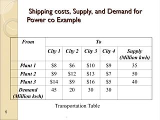
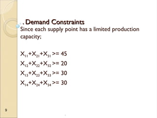
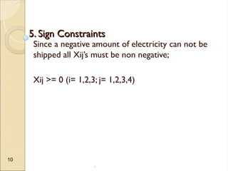
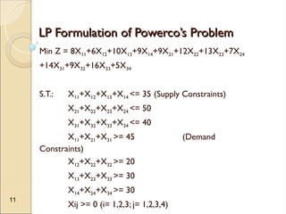
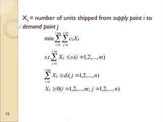
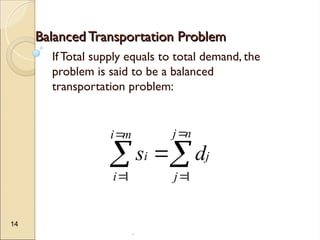
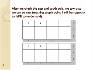
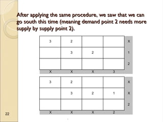
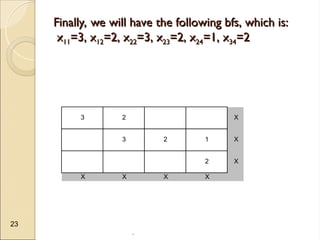
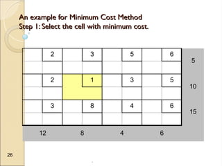
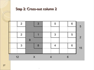
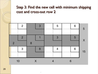
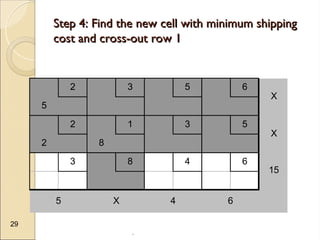
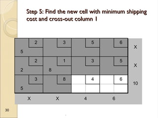
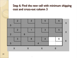
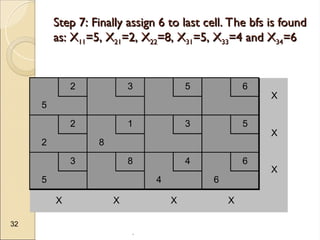
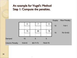
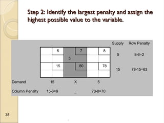
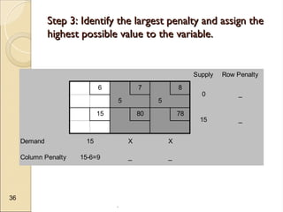
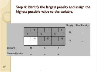
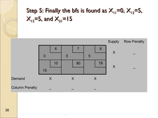
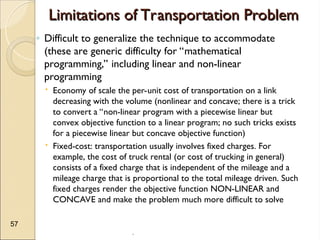
The document discusses transportation problems, which involve optimizing the distribution of goods from multiple supply points to various demand points while minimizing shipping costs. It describes methods for formulating and solving these problems, including the Northwest Corner Method, Minimum Cost Method, and Vogel’s Method, along with a practical example using electric power distribution. Additionally, the document touches upon assignment problems with a focus on minimizing setup times for job assignments to machines.

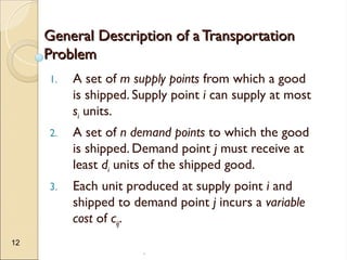


![ANIMAL_CELL_,_TISSUE_AND_ORGAN_CULTURE[1].pptx](https://cdn.slidesharecdn.com/ss_thumbnails/animalcelltissueandorganculture1-260204172026-4462b440-thumbnail.jpg?width=640&height=640&fit=bounds)


