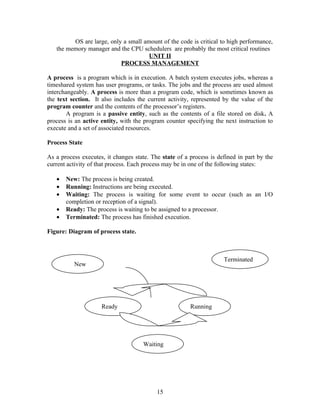
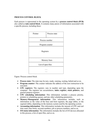
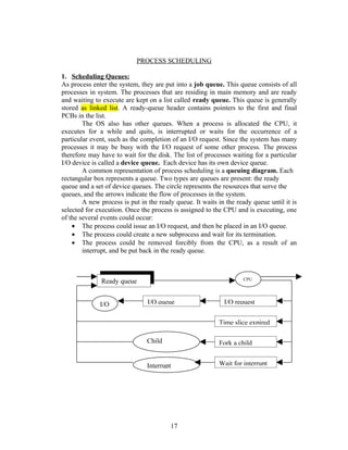
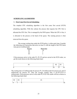
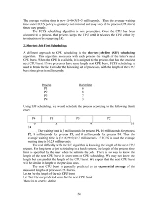
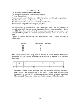
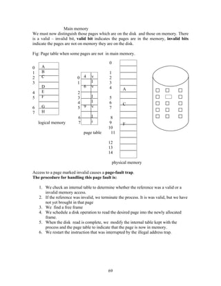
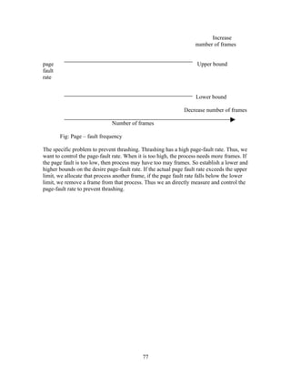
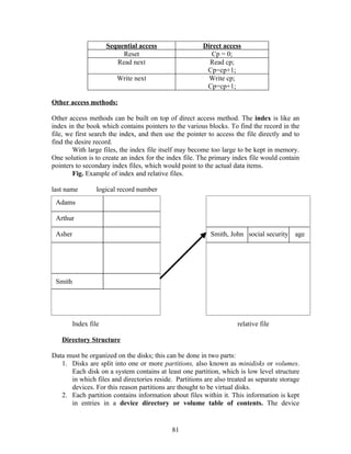
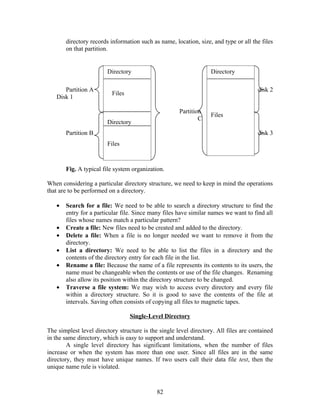
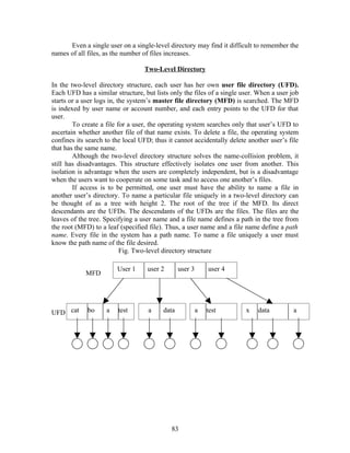
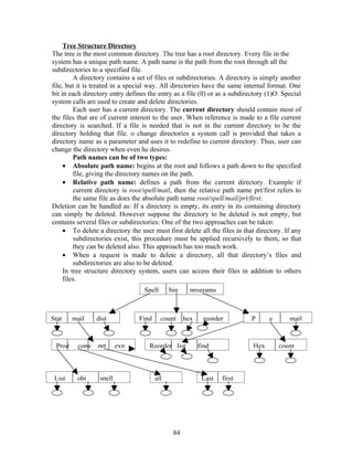
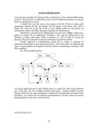
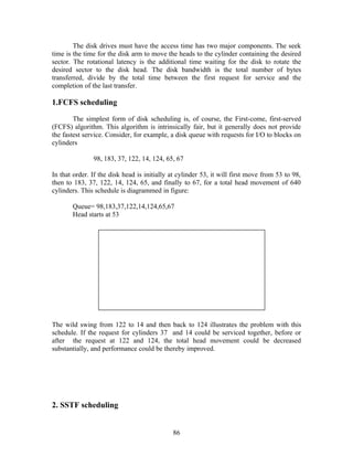
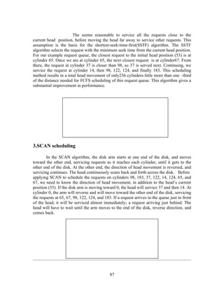
The document discusses the evolution of operating systems from mainframe to desktop and distributed systems. It describes [1] how mainframe systems used batch processing and multiprogramming to improve CPU utilization, [2] how time-sharing systems enabled interactive use by rapidly switching between users, [3] how personal computers led to single-user desktop systems like MS-DOS and Windows, and [4] how distributed systems employ client-server and multiprocessing architectures to share resources over networks.

1. UNIT – I
INTRODUCTION
Operating system is a program that manages the computer hardware. It also provides a
basis for application programs and acts as an intermediary between a user of a computer
and the computer hardware. An operating system is an important part of almost every
computer system. A computer system can be divided roughly into four components:
• The hardware – the central processing unit (CPU), the memory, and the
input/output (I/O) devices provides the basic computing resources.
• The operating system - controls and coordinates the use of the hardware among
the various application programs for the various users.
• Application programs – such as word processors, spreadsheets, compilers, and
web browsers define the way in which these resources are used to solve the
computing problems of the users.
• Users.
MAINFRAME SYSTEMS
Mainframe computer systems were the first computers used to tackle many commercial
and scientific applications.
1.Batch Systems
The user did not interact directly with the computer systems. They prepared a job which
consisted of the program, the data, and some control information about the nature of the
job and submitted it to the computer operator. After some days the output appeared. The
output consisted of the result of the program. The major task was to transfer control
automatically from one job to next.
To speed up processing, operators batched together jobs with similar needs and
ran them through the computer as a group. Thus the programmers leave their programs
with the operator. The operator would sort programs into batches with similar
requirements and, as the computer became available, would run each batch. The output
from each job would be sent back to the appropriate programmer.
2.Multiprogrammed Systems
Multiprogramming increases CPU utilization by organizing jobs so that the CPU
always has one to execute.
The concept of multiprogramming is that the operating system keeps several jobs in
memory simultaneously. This set of jobs are kept in the job pool. The OS picks up and
execute one of the jobs in the memory.
• In non-multiprogramming system, the CPU would sit idle.
• In multiprogramming system, the OS simply switches to, and executes, another
job. When that job needs to wait, the CPU is switched to another job, and so on.
The first finishes waiting and gets the CPU back. As long a at least one job needs
to execute, the CPU is never idle.
1

2. Multiprogramming operating systems are used for decisions for the users. All the jobs
that enter the system are kept in the job pool. This pool consists of all processes residing
on disk awaiting allocation of main memory. If several jobs are ready to be brought into
memory, and if there is not enough room for all of them, then the system must choose
among them. Making this decision is job scheduling. If several jobs are ready to run at
the same time, the system must choose among them, this decision is CPU scheduling.
3.Time – Sharing Systems
Time sharing or multitasking is a logical extension of multiprogramming. The CPU
executes multiple jobs by switching among them, but the switches occur so frequently
that the users can interact with each program while it is running.
An interactive (or hands-on) computer system provides direct communication between
the user and the system. The user gives instructions to the operating system or to a
program directly, using a keyboard or a mouse, and waits for immediate results.
A time-shared operating system allows many users to share the computer
simultaneously. Each action or command in a time –shared system tends to be short, only
a little CPU time is needed for each user. As the system switches rapidly from one user
to the next, each user is given the impression that the entire computer system is dedicated
to her use, even though it is being shared among many users.
A time-shared operating system uses CPU scheduling and multiprogramming to
provide each user with a small portion of a time-shared computer. Each user has atleast
one separate program in memory. A program loaded into memory and executing is
commonly referred to as a process. When a process executes, it typically executes for
only a short time before it either finishes or needs to perform I/O.
DESKTOP SYSTEMS
Personal computers PCs appeared in the 1970s. During their first decade, the CPUs in
PCs lacked the features needed to protect an operating system from user programs. PC
operating systems therefore were neither multiuser nor multitasking. The MS-DOS
operating system from Microsoft has been produced multiple flavors of Microsoft
Windows, and IBM has upgraded MS-DOS to OS/2 multitasking system. UNIX is used
for its scalability, performance, and features but retains the same rich GUI. Linux, a
UNIX operating system available for PCs, has also become popular recently.
OS has developed for mainframes. Micro computers were able to adopt some of
the technology developed for larger OS. On the other hand, the hardware costs for micro
computers are sufficiently low that individuals have sole use of the computer, and the
CPU utilization is no longer a prime concern.
Earlier file protection was not necessary on a personal machine. But these
computers are now often tied into other computers over local-area networks or other
Internet connections. When other computers and other users can access the files on a PC,
file protection becomes essential feature of the operating system. The lack of such
protection has made it easy for malicious programs to destroy data on the systems such as
MS-DOS and the Macintosh operating system. These programs are self-replicating, and
may spread rapidly via worm or virus mechanism.
2

3. MULTIPROCESSOR SYSTEMS
Multiprocessor systems have more than one processor or CPU. Multiprocessor systems
also known as parallel systems. Such systems have more than one processor in close
communication, sharing the computer bus, the clock, and sometimes memory and
peripheral devices.
Advantages of the multiprocessor systems are:
1. Increased throughput: By increasing the number of processors, get more work
done in less time. When multiple processors cooperate on a task, a certain amount
of overhead is incurred in keeping all the parts working correctly.
2. Economy of scale: Multiprocessor systems can save more money than multiple
singe-processor systems, because they can share peripherals, mass storage, and
power supplies. If several programs operate on the same set of data, it is cheaper
to store those data on one disk and to have all the processors share them, than to
have many computers with local disks and many copies of the data.
3. Increased reliability: If functions can be distributed properly among several
processors, then the failure of one processor will not halt the system, only slow it
down.
The most common multiple-processor systems now use symmetric multiprocessing
(SMP), in which each processor runs on identical copy of the OS, and these copies
communicate with one another as needed. Some systems use asymmetric
multiprocessing, in which each processor is assigned a specific task. A master processor
controls the system, the other processors either look to the master for instruction or have
predefined tasks. This scheme defines a master-slave relationship. The master processor
schedules and allocates work to the slave processors.
Figure: Symmetric multiprocessing architecture
CPU CPU
CPU
memory
SMP means that all processors are peers, no master-slave relationship exists between
processors. Each processor concurrently runs a copy of the operating system. The benefit
of this model is that many processes can run simultaneously - N processes can run if
there a N CPUs- without causing a significant performance. Since the CPU are separate,
one may be sitting idle while another is overloaded, resulting in inefficiencies. A
multiprocessor system will allow processors and resources-such s memory to be shared
among the various processors.
3

4. DISTRIBUTED SYSTEMS
A network, in the simplest terms, is a communication path between two or more
systems. Distributed systems depend on networking for their functionality. Distributed
systems are able to share computational tasks, and provide a rich set of features to users.
Networks are typecast based on the distance between their nodes.
• Local area network: exists within a room, a floor, or a building.
• Wide area network: exists between building, cities, or countries. A global
company may have a WAN to connect its offices, world wide.
• Metropolitan are network: could link buildings within a city.
1.Client – Server Systems:
client client client client
server
Terminals connected to centralized systems are now being supplanted by CPU.
Centralized systems today act as server systems to satisfy requests generated by client
systems.
Server systems can be broadly categorized as compute servers and file servers.
• Compute-server systems: provide an interface to which clients can send requests
to perform an action, in response to which they execute the action and send back
results to the clients.
• File-server systems: provide a file-system interface where clients can create,
update, read and delete files.
2.Peer-to-Peer Systems
The growth of computer networks especially the Internet and WWW has a profound
influence on the recent development of OS. When PCs were introduced in 1970s they
were developed as stand alone systems, but with the widespread public use of the Internet
in 1980s for electronic mail, ftp, PCs became connected to computer networks.
Modern PCs and workstations are capable of running a web browser for accessing
hypertext documents on the web. The PCs now include software that enables a computer
to access the Internet via a local area network or telephone connection. These systems
consist of collection of processors that do not share memory or a clock. Instead each
processor has its own local memory. The processors communicate with another through
various communication lines, such as high speed buses or telephone line.
OS has taken the concept of network and distributed systems for network
connectivity. A network operating systems is an OS that provides features such as file
sharing across the network, and that includes a communication scheme that allows
different processes on different computers to exchange messages.
4

5. CLUSTERED SYSTEMS
Clustered systems gather together multiple CPUs to accomplish computational work.
Clustered systems differ from parallel system, in that they are composed of two or more
individual systems coupled together. Clustering is usually performed to provide high
availability. A layer of cluster software runs on the cluster nodes. Each node can monitor
one or more o the others. If the monitored machine fails, the monitoring machine can take
ownership of its storage, and restart the application that were running on the failed
machine. The failed machine can remain down, but the users and clients of the
application would only see a brief interruption of service.
In asymmetric clustering, one machine is in hot standby mode when the other
is running the applications. The hot standby machine does nothing but monitor the active
server. If that server fails, the hot standby host becomes the active serer.
In symmetric clustering, two or more nodes are running applications, and they
are monitoring each other. This mode is more efficient, as it uses all o the available
hardware.
Parallel clusters allow multiple hosts to access the same data on the shared
storage. Because most of the operating systems lack support for simultaneous data access
by multiple hosts, parallel clusters are usually accomplished by special versions of
software. Example Oracle parallel server is a version of Oracle’s database that has been
designed to run on parallel clusters.
REAL-TIME SYSTEMS
A real time system is used when rigid time requirements have been placed on
the operation of a processor or the flow of data; thus it is used as a control device in a
dedicated application. Sensors bring data to the computer. Computer must analyze the
data and possibly adjust controls to modify the sensor inputs. Systems that control
scientific experiments, medical imaging systems, industrial control systems, some
automobile-engine fuel-injection systems, home appliance controllers and weapon
systems are also real time systems.
A real-time system has well-defined, fixed time constraints. Processing must be
done within the defined constraints, or the system will fail. A real time systems functions
correctly only if it returns the correct result within its time constraints.
Real time systems if of two types:
• A hard real time system guarantees that critical tasks be completed on time. This
goal requires that all delays in the system be bounded, from the retrieval of stored
data to the time that it takes the operating system to finish any request made of it.
• A soft real time system where a critical real time task gets priority over those
tasks, and retains that priority until it completes. An in hard real-time systems, the
OS kernel delays need to be bounded: A real-time task cannot be kept waiting
indefinitely for the kernel to run it. They are useful in several areas, including
multimedia, virtual reality, and advanced scientific projects such as undersea
exploration and planetary rovers. These systems needs advanced operating
systems.
5

6. HANDHELD SYSTEMS
Handheld systems include personal digital assistants(PDAs), such as Palm pilots
or cellular telephones with connectivity to a network such as the Internet. The
handheld systems are of limited size. Example, a PDA is typically 5 inches in height
and 3 inches in width, and weighs less than one-half pound. Due to its limited size,
handheld systems have a small amount of memory, include slow processors, and
feature small display screens. They have between 512 KB and 8 MB of memory.
The next issue is the handheld devices is the speed of the processor used in the
device. Processors of handheld devices often run at a fraction of the speed of a
processor in a PC. Faster processors require more power. To include a faster
processor in a handheld device would require a larger battery that would have to be
replaced more frequently.
The last issue for the designers for handheld devices are handheld devices is
the small display screens typically available. Whereas a monitor for a home computer
may measure up to 21 inches, the display for a handheld device is often no more than
3 inches square. Tasks such as reading e-mail or browsing web pages, must be
condensed onto the smaller displays. One approach for displaying the content in web
pages is web clipping, where only a small subset of a web page is delivered and
displayed on the handheld device.
Some handheld devices may use wireless technology, such as BlueTooth,
allowing remote access to e-mail and web browsing. Cellular telephones with
connectivity to Internet fall into this category. To download data to these devices,
first the data is downloaded to a PC or workstation, and then downloads the data to
the PDA. Some PDAs allow data to be directly copied from one device to another
using an infrared link.
OPERATING SYSTEM STRUCTURES
An operating system may be viewed from several points.
1. By examining the services that it provides.
2. By looking at the interface that it makes available to users and programmers.
3. By disassembling, the system into its components and their interconnections.
OPERATING SYSTEM COMPONENTS:
The various system components are:
1. Process management
2. Main-memory management
3. File management
4. I/O-system management
5. Secondary-storage management
6. Networking
7. Protection system
8. Command-Interpreter system
6

7. 1. Process Management
A Process is thought as a program in execution. A program does nothing unless
its instructions are executed by a CPU. Example, a compiler is a process, a word
processing program run by an individual user on a PC is a process, a system task,
such as sending output to a printer is also a process.
A process needs certain resources including CPU time, memory, files and
I/O devices to accomplish its task. These resources are either given to the process
when it is created or allocated to it while it is running. A program is a passive
entity, such as the contents of the file stored on disk, whereas a process is an
active entity, with a program counter specifying the next instruction to be
executed. The execution of the process must be sequential. The CPU executes
one instruction of the process after another, until the process completes.
A process is the unit of work in a system. Such a system consists of
collection of processes, some of which are operating system processes and the rest
are user processes.
The OS is responsible for the following activities in process management:
• Creating and deleting both user and system processes
• Suspending and resuming processes
• Providing mechanisms for process synchronization
• Providing mechanisms for process communication
• Providing mechanisms for deadlock handling
2. Main-Memory Management
Main memory is a repository of quickly accessible data shared by the CPU and I/
O devices. The central processor reads the instructions from main memory during
the instruction fetch cycle, and it reads instructions from main memory during the
data fetch cycle.
The main memory is the only larger storage device the CPU able to
address and access directly. For a program to be executed, it must be mapped to
absolute addresses and loaded into memory. As the program executes, it accesses
program instructions and data from memory by generating theses absolute
addresses. To improve the CPU utilization and the speed of the computer’s
response to its users, we must keep several programs in memory.
The OS is responsible for the following activities in memory management:
• Keeping track of which parts of memory are currently being used and
by whom
• Deciding which processes are to be loaded into memory when memory
space becomes available.
• Allocating and deallocating memory space as needed.
7

8. 3. File Management
A File is a collection of related information defined by its creator. Files define
programs and data. Data files can be numeric, alphabetic and alphanumeric. Files
may be of free form, or may be formatted rigidly. A file consists of sequence of
bits, bytes, lines or records whose meanings are defined by their creators. Files are
organized into directories to ease of their use. Files can be opened in different
modes to be accessed, they are : read, write, append.
The OS responsibilities for the following activities for file management :
• Creating and deleting files
• Creating and deleting directories
• Supporting primitives for manipulating files and directories
• Mapping files onto secondary storage
• Backing up files on stable, nonvolatile storage media
4. I/O System Management
One of the purposes of an operating system is to hide the attributes and characters
of specific hardware devices for the user.
The I/O subsystem consists of:
• A memory-management component that includes buffering, caching,
and spooling
• A general device-driver interface
• Drivers for specific hardware devices
The device drivers alone know the characteristics of the specific device to which
it is assigned.
5. Secondary-Storage Management
The main purpose of the computer system is to execute the programs. These
programs, with the data they access, must be in main memory, or primary
memory, during execution. Because the main memory is too small to hold all the
data and programs, and as the data it holds is lost when the power is lost, the
computer must provide secondary storage to back up main memory. Programs
such as compilers, assemblers, routines, editors and formatters are stored in
the disk until loaded into main memory.
The OS responsibility for the following activities for disk management:
• Free-space management
• Storage allocation
• Disk scheduling
8

9. 6. Networking
A distributed system is a collection of processors that do not share memory,
peripheral devices, or a clock. Each processor has its own local memory and clock,
and the processors communicate with one another through various communication
lines, such as high-speed buses or networks. The processors in distributed system
vary in size and function. They include small micro-processors, workstations,
minicomputers and large, general purpose computer systems.
A distributed system collects physically separate, and many heterogeneous
systems into a single coherent system, providing user with access to the various
resources that the system maintains. The shared resources allows computation
speedup, increased functionality, increased data availability, and reliability.
Different protocols are used in the network system, such as file-transfer
protocol (FTP), Network file-system (NFS), hypertext transfer protocol (HTTP) ,
for use in communication between a web server and a web browser. A web browser
then just needs to send a request for information to a remote machines web server.
And the information is returned.
7. Protection System
If a computer system has multiple users and allows the concurrent execution of
multiple processes, then the various processes must be protected from the other
process.
Protection is any mechanism for controlling the access of programs,
processes, or users to the resources defined by a computer system. This mechanism
must provide means for specification of the controls to be imposed and means for
enforcement.
Protection can improve reliability by detecting latent errors at the interfaces
between component subsystems. Early detection of interface errors can often prevent
contamination of a healthy subsystem by another subsystem. Unprotected system can
be used by unauthorized users.
8. Command-Interpreter System
Command interpreter is an interface between the user and the operating system.
Many commands are given to the operating system by control statements. When a
new job is started in a batch system, or when a user logs on to a time-shared system, a
program that reads and interprets control statement is executed automatically. This
program is sometimes called the control card interpreter or command-Interpreter,
and is often known as the shell. Its function is to get the next command statement and
execute it.
9

10. OPERATING SYSTEM SERVICES
An operating system provides an environment for the execution of programs. It
provides certain services to programs and to the users of those programs.
The various services offered by Operating system are:
• Program execution: The system may be able to load a program into memory
and to run that program. The program must be able to end its execution, either
normally or abnormally indicating the error.
• I/O operations: A running program may require I/O. This I/O may involve a
file or an I/O device. For security and efficiency users usually cannot control
I/O devices directly, operating system must be provided to do it.
• File-system manipulation: The files needs programs to read and write files.
Programs also need to create and delete files by names.
• Communications: One process needs to communicate with another process.
Such communication may occur in two ways:
o Communication takes place between processes that are executing on
the same computer.
o Takes place between processes that are executing on different
computer systems that are tied together by a computer network.
Communications may be implemented via shared memory, or by the
technique of message passing, in which packets of information are
moved between processes by the operating system.
• Error detection: The operating system constantly needs to be aware of
possible errors. Errors may occur in :
o the CPU and memory hardware-memory error or power failure.
o I/O devices-such as parity error on tape, a connection failure on
network, or lack of paper in the printer.
o User program-an arithmetic overflow, an attempt to access an illegal
memory location, or too great use of CPU time.
• Resource allocation: When multiple users are logged on the system, multiple
jobs are running at the same time, resources must be allocated to all of them.
Many different types of resources are managed by the operating system. Some
are CPU cycles, main memory, and file storage may have special allocation
code, and I/O devices may have general request and release code.
• Accounting: Os must keep track of which users use how many and which
kinds of computer resources.
• Protection: The owners of the information stored in a multiuser computer
system may want to control use of the information. When several processes
are executed concurrently, one process should not interfere with the other
process. Security of the system from outsiders is also important. Such
security starts with each user having to authenticate himself to the system ,
usually by means of a password, to be allowed access to the resources.
10

11. SYSTEM CALLS
System calls provide the interface between a process and the operating system. These
calls are usually available as assembly-language instructions and they are listed in
manuals for programmers. Several systems allow system calls to be available in high
level languages. Several languages such as C, C++, Perl have replaced assembly
language for system programming. Example, UNIX system calls may be invoked
directly from a C or C++ program.
System calls can be grouped into five major categories:
1) Process Control:
A running program needs to be able to halt its execution either normally or
abnormally. If a system call is made to terminate the currently running program
abnormally. Either normal or abnormal , the operating system must transfer control to
the command interpreter. The command interpreter then reads the next command.
The command interpreter reads the next instruction.
A process or job executing one program may want to load and execute other
program. An interesting question is where to return control when the loaded program
terminates. Whether the existing program is lost, saved, or allowed to continue
execution concurrently with the new program.
If control returns to the existing program when the new program terminates,
we must save the memory image of the existing program. If both programs continue
concurrently, we have created a new job or process to be multiprogrammed. System
calls for this purpose is create process or submit job.
If a new job or process is created, we may need to wait for them for some time
to finish their execution. We may want to wait for a certain amount of time (wait
time), we may want to wait or a specific event to occur (wait event). The jobs or
processes should then signal when that event has occurred (signal event).
If we create a new job or processes, we should be able to execute it. This
control requires the ability to determine and reset the attributes of a job or process,
including the job’s priority, its maximum allowable execution time, (get process
attributes and set process attribute).
Another set of system calls is helpful in debugging a program. Many systems
provide system calls to dump memory. This provision is useful for debugging. A
program trace lists each instruction as it is executed; it is provided by fewer systems.
The trap is usually caught by a debugger, which is a system program designed to aid
the programmer in finding and correcting bugs.
2) File Management
The files must be created and deleted. Either system calls requires the name of the
file and some of the attributes. Once the file is created, it must be open and used. It
11

12. may also read, write and reposition (rewind or skip to the end of the file). Finally the
file need to be closed.
File attributes include the file name, a file type, protection codes, accounting
information and so on. The system calls for this purpose are get file attribute and set
file attribute.
3) Device Management
A program running, may need additional resources to proceed. The resources may be
more memory, tape drivers, access to files. If the resources are available, they can be
granted and control can be returned to the user program; otherwise the program will
have to wait until sufficient resource are available.
Once the device has been requested (an allocating to us), we can read, write,
and reposition the device.
4) Information Maintenance
Many system calls exist simply for the purpose of transferring information between
the user program and the operating system. For example, systems have a system call
to return the current time and date. Other system calls may return information about
the system, such as the number of current users, the version number of the operating
system, the amount of free memory or disk space.
There are system calls to access these information. They are get process
attributes and set process attributes.
5) Communication
There are two common models of communication. In message-passing model,
information is exchanged through an interprocess communication. Before
communication can take place, a connection must be opened. The name of the other
communicator must be known, bit it another process on the same PU, or a process on
another computer connected by networks. Each computer in the network has a host
name, such as IP name. Similarly each process has a process name.
The get hosted and get processed system calls do this process. These identifiers
are then passed to specific open connection and close connection system calls. The
recipient process usually must give its permission for communication to take place
with an accept connection call. Most processes that will be receiving connection are
special purpose daemons. They execute a wait for connection call and are awakened
when a connection is made. The source of the communication, known as the client,
and the receiving daemon, known as server, then exchange messages by read message
and write message system calls. The close connection terminates the communication.
In shared-memory model, processes may exchange information by reading
and writing data in these processes and are not under the operating systems control.
12

13. SYSTEM PROGRAMS
System program provide a convenient environment for program development and
execution. They can be divided into these categories:
• File Management
These programs create, delete, copy, rename, print, dump, list and generally
manipulate files and directories.
• Status information
Some programs simply ask the system for the date, time, amount of available
memory or disk space, number of users, or similar status information. That
information is then formatted, and printed to the terminal or other output
device or file.
• File modification
Several text editors may be available to create and modify the content of the
files stored on disk or tape.
• Programming language support
Compilers, assemblers, and interpreters for common programming languages
such a C, C++, java, Visual Basic are often provided to the user with the
operating system. Some of these programs are now priced and provided
separately.
• Program loading and execution
Once a program is assembled or compiled, it must be loaded into memory to
be executed. Debugging systems for either higher-level languages or machine
language are needed.
• Communications
These programs provide the mechanism for creating virtual connections
among processes, users, and different computer systems. They allow users to
send messages to one another’s screens, to browse web pages, to send e-mail
messages, to log remotely, or to transfer data files from one machine to
another.
13

14. SYSTEM DESIGN AND IMPLEMENTATION
1. Design Goals
The first problem in designing a system is to define the goals and specification of the
system. The design of the system will be affected by the choice of hardware and type
of system: batch, time shared, single user, multiuser, distributed, real time, or general
purpose.
Requirement can be divided into two basic groups:
• User goals
• System goals
User desire certain properties in a system: The system should be convenient and easy
to use, easy to learn, reliable, safe, and fast. Similarly a set of requirements can be
defined by those people who must design, create, implement and maintain; it should
be flexible, reliable, error free, and efficient.
2. Mechanisms and Policies
One important principle is the separation of policy from mechanism. Mechanism
determines how to do something; policies determine what will be done. Example, the
timer construct is a mechanism for ensuring CPU protection, but deciding how long
the timer is to be set for a particular user is a policy decision.
Policies are likely to change across places or overtime. In worst case, each
change in policy would require a change in the underlying mechanisms. A change in
policy would require redefinition of only certain parameters of the system. For
instance, if one computer system, a policy decision is made that I/O intensive
programs should have priority over CPU intensive ones, then the opposite policy
could be instituted easily on some other computer systems if the mechanism were
properly separated and were policy independent.
3. Implementation
Once an operating system is designed, it must be implemented. Traditionally, OS
were written in assembly language. Now they are often written in higher-level
languages as C, C++.
The various operating systems not written in assembly language are:
• The Master Control Program (MCP), it was written in ALGOL.
• MULTICS, developed at MIT, was written in PL/1.
• The Primos operating system for Prime computers is written in Fortran.
• The UNIX operating system, OS/2, and Windows NT are written in C.
The advantages of writing OS in higher-level language are the code can be
written faster, is more compact, and is easier to understand and debug. The OS is far
easier to port to move to some other hardware if it is written in high-level language.
The disadvantage of writing OS in high-level language is the reduced speed
and increased storage requirements.
14

15. OS are large, only a small amount of the code is critical to high performance,
the memory manager and the CPU schedulers are probably the most critical routines
UNIT II
PROCESS MANAGEMENT
A process is a program which is in execution. A batch system executes jobs, whereas a
timeshared system has user programs, or tasks. The jobs and the process are used almost
interchangeably. A process is more than a program code, which is sometimes known as
the text section. It also includes the current activity, represented by the value of the
program counter and the contents of the processor’s registers.
A program is a passive entity, such as the contents of a file stored on disk. A
process is an active entity, with the program counter specifying the next instruction to
execute and a set of associated resources.
Process State
As a process executes, it changes state. The state of a process is defined in part by the
current activity of that process. Each process may be in one of the following states:
• New: The process is being created.
• Running: Instructions are being executed.
• Waiting: The process is waiting for some event to occur (such as an I/O
completion or reception of a signal).
• Ready: The process is waiting to be assigned to a processor.
• Terminated: The process has finished execution.
Figure: Diagram of process state.
Terminated
New
Ready Running
Waiting
15

16. PROCESS CONTROL BLOCK
Each process is represented in the operating system by a process control block (PCB)
also called as task control block. It contains many pieces of information associated with
a specific process, including these:
Pointer Process state
Process number
Program counter
Registers
Memory lines
List of open files
….
….
Figure: Process control block
• Process state: The state may be new, ready, running, waiting, halted and so on.
• Program counter: The counter indicates the address of the next instruction to be
executed.
• CPU registers: The registers vary in number and type, depending upon the
computer. The registers are accumulators, index register, stack pointers, and
general purpose registers.
• CPU scheduling information: This information includes a process priority,
pointers to scheduling queues, and any other scheduling parameters.
• Memory-Management information: This information includes such as
information as the value of the base and limit registers, the page tables, or the
segment tables, depending on the memory system used by the operating system.
• Accounting information: This information includes the amount of CPU and real
time used, time limits, account numbers, job or process numbers, and so on.
• I/O status information: The information includes the list of I/O devices allocated
to this process, a list of open files, and so on.
16

17. PROCESS SCHEDULING
1. Scheduling Queues:
As process enter the system, they are put into a job queue. This queue consists of all
processes in system. The processes that are residing in main memory and are ready
and waiting to execute are kept on a list called ready queue. This queue is generally
stored as linked list. A ready-queue header contains pointers to the first and final
PCBs in the list.
The OS also has other queues. When a process is allocated the CPU, it
executes for a while and quits, is interrupted or waits for the occurrence of a
particular event, such as the completion of an I/O request. Since the system has many
processes it may be busy with the I/O request of some other process. The process
therefore may have to wait for the disk. The list of processes waiting for a particular
I/O device is called a device queue. Each device has its own device queue.
A common representation of process scheduling is a queuing diagram. Each
rectangular box represents a queue. Two types are queues are present: the ready
queue and a set of device queues. The circle represents the resources that serve the
queues, and the arrows indicate the flow of processes in the system.
A new process is put in the ready queue. It waits in the ready queue until it is
selected for execution. Once the process is assigned to the CPU and is executing, one
of the several events could occur:
• The process could issue an I/O request, and then be placed in an I/O queue.
• The process could create a new subprocess and wait for its termination.
• The process could be removed forcibly from the CPU, as a result of an
interrupt, and be put back in the ready queue.
CPU
Ready queue
I/O I/O queue I/O request
Time slice expired
Child Fork a child
executes
Interrupt Wait for interrupt
17

18. 2. Schedulers
A process migrates between the various scheduling queues throughout its lifetime.
The operating system must select, for scheduling purposes, processes from these
queues in some fashion. The selection process is carried out by the appropriate
scheduler. There are two types of schedulers:
• Long-term schedulers or job schedulers: This selects processes from
job pool and loads them into memory for execution.
• Short-term scheduler or CPU scheduler: This selects among the
processes that are ready to execute and allocates the CPU to one of them.
The primary difference between these two schedulers is the frequency of their
execution. The short-term scheduler must select a new process for the CPU
frequently. A process may execute for only a few milliseconds therefore waiting for
an I/O request. This often executes once in every 100 milliseconds.
The long-term scheduler on the other hand, executes much less frequently.
There may be minutes between the creations of new processes in the system. The
long-term schedulers are needed to be invoked only when the process leaves the
system.
On some systems, such as time sharing systems, may introduce an additional,
intermediate level of scheduling. This medium-term scheduler removes processes
from memory, and thus reduces the degree of multiprogramming. At some later time,
the process can be reintroduced into memory and its execution can be continued
where it left off. This scheme is called swapping. The process is swapped out, and is
later swapped in, by the medium-term scheduler.
3. Context Switch
Switching the CPU to another process requires saving the state of the old process and
loading the saved state for the new process. This task is known as a context switch.
The context of a process is represented in the PCB of a process; it includes the value
of the PU registers, the process state and memory management information. When a
context switch occurs the Kernel saves the context of the old process in its PCB and
loads the saved context of the new process scheduled to run. Context switch is pure
overhead, because the system does no useful work while switching. Its speed varies
from machine to machine, depending on the memory speed, the number of registers
that must be copied, and the existence of special instructions. The speed ranges from
1 to 1000 milliseconds.
OPERATIONS ON PROCESSES
The processes in the system can execute concurrently, and they must be created and
deleted dynamically. Thus the operating system must provide a mechanism for process
creation and termination.
18

19. 1. Process Creation
A process may create several new processes, via create-process system call during
the execution. The creating process is called a parent process, whereas the new
processes are called children of that process. Each of these new processes may in
turn create other processes, forming a tree structure.
A process needs certain resources such as CPU time, memory, files, I/O
devices to accomplish any task. When a process creates a sub process may be able to
obtain its resources directly from the operating system, or the parent may have to
partition its resources among its children.
Example: Consider a process whose function is to display the status of a file,
say F1, on the screen of the terminal. When it is created, it will get as an input from
its parent process, the name of the file F1, and it will execute using that datum to
obtain the desired information. It may also get the name of the output device.
When a process creates new process, two possibilities exist in terms of
execution:
1. The parent continues to execute concurrently with its children.
2. The parent waits until some or all of its children have terminated.
3. Process Termination
A process terminates when it finishes executing its final statement and asks the
operating system to delete it by using the exit system call. At that point the process
may return data output to its parent process via a wait system call.
A process can cause termination of another process via an appropriate system
call. When a process is newly created, the identity of the newly created process is
passed to its parent.
A parent may terminate the execution of one of its children for a variety of
reasons, such as:
• The child has exceeded its usage of some of the resources that it has been
allocated. This requires the parent to have a mechanism to inspect the state of
its children.
• The task assigned to the child is no longer required.
• The parent is exiting, and the operating system does not allow a child to
continue if its parent terminates. On such systems, if a process terminates then
all its children must also be terminated. This phenomenon is called as
cascading termination.
COOPERATING PROCESSES
The concurrent processes executing in the operating system may either be independent
processes or cooperating processes. A process is independent if it cannot affect or be
affected by other processes executing in the system. The process that does not share any
data with any other process is independent. A process is cooperating if it can affect or be
affected by the other processes is a cooperating process.
19

20. Process cooperation is provided for several reasons:
• Information sharing: Since several users may be interested in the same piece of
information, we must provide an environment to allow concurrent access to these
types of resources.
• Computation speedup: If we want a particular task to run faster, we must break
it into subtasks, each of which will be executing in parallel with the others. Such
speedup can be achieved only if the computer has multiple processing elements.
• Modularity: We may want to construct the system in a modular fashion, dividing
the system functions into separate processes or threads.
• Convenience: Even an individual user may have many tasks on which to work at
one time. For instance, a user may be editing, printing, and compiling in parallel.
To illustrate the concept of cooperating processes, consider the producer-consumed
problem. A producer process produces information that is consumed by a consumer
process. Example, a print program produces characters that are consumed by the
printer device. A compiler may produce assembly code, which is consumed by an
assembler. The assembler, in turn, may produce object modules, which are consumed
by the loader.
To allow producer and consumer processes to run concurrently, we must have
available a buffer of items that can be filled by producer and emptied by the
consumer. A producer can produce one item while the consumer is consuming
another item. The producer and the customer must be synchronized so that the
consumer does not try consuming an item that has not yet produced.
INTERPROCESS COMMUNICATION
IPC provides a mechanism to allow processes to communicate and to synchronize their
actions without sharing the same address space. IPC is particularly useful in a distributed
environment where the communicating processes may reside on different computers
connected with a network. An example is the chat program used on WWW.
1. Message Passing System
The function of a message system is to allow processes to communicate with one another
without the need to resort to the shared data. Communication among the user processes is
accomplished through the passing of message. An IPC facility provides at least the two
operations: Send(message) and receive(message).
Messages sent by7 a process can be of either fixed size or variable size. If
processes P and Q want to communicate they must send messages to and receive
messages from each other; a communication link must exist between them. This link can
be implemented in a variety of ways. We are concerned not with physical
implementation(such as shared memory, hardware, bus or network) but rather with its
logical implementation. Here are several methods for logically implementing a link and
the send / receive operations:
• Direct or indirect communication
• Symmetric or asymmetric communication
20

21. • Automatic or explicit buffering
• Send by copy or send by reference
• Fixed-sized or variable-sized messages.
Naming
1. Direct Communication:
With direct communication, each process that wants to communicate must
explicitly name the recipient or sender of the communication. In this scheme the send
and the receive primitives are:
• Send (P, message) – Send a message to process P.
• Receive(Q, message) – receive a message from process Q
A communication link in this scheme has the following properties:
• A link is established automatically between every pair of processes that want to
communicate. The processes need to know only each other’s identity to
communicate.
• A link is associated with exactly two processes.
• Exactly one link exists between each pair of processes.
This scheme exhibits symmetry in addressing, that is both the sender and the receiver
processes must name the other to communicate. A variant of this scheme employs
asymmetric in addressing. Only the sender names the recipient; the recipient is not
required to name the sender. In this scheme the send and receive primitives are defined as
follows:
• Send (P, message) – send a message to process P
• Receive(id, message) – receive a message from any process, the variable id is set
to the name of the process with which communication has taken place.
2. Indirect Communication:
With indirect communication, the messages are sent to and received from
mailboxes, or ports. A mailbox can be viewed abstractly as an object into which
message can be placed by processes and from which messages can be removed. Each
mailbox has a unique identification. In this scheme a process can communicate with some
other process via a number of different mailboxes. Two processes can communicate only
if they share a mailbox. The send and receive primitives are defined as follows:
• Send (A, mailbox) – send a message to mailbox A
• Receive(A, message) – receive a message from mailbox A
In this scheme, a communication link has the following property:
• A link may be associated with more than two processes.
21

22. • A number of different links may exist between each pair of communicating
processes, with each link corresponding to one mailbox.
Mailbox can be owned by either by a process or by the operating system. If the mailbox
is owned by a process, then each owner is distinguished (who can receive the message)
and the user( who send the messages). Since each mailbox has a unique owner, there can
be no confusion about who should receive the message sent to the mailbox. When a
process that owns a mailbox terminates, the mailbox disappears. Any process that
subsequently sends a message to this mailbox must be notified that the mailbox no longer
exists.
On the other hand, a mailbox owned by the operating system is independent and
is not attached to any particular process. The operating system then must provide a
mechanism that allows a process to do the following:
• Create a new mailbox
• Send and receive messages through the mailbox
• Delete a mailbox.
3. Synchronization:
Communication between processes takes place by calls to send and receive primitives.
Message passing may be either blocking or non-blocking also known as synchronous
and asynchronous.
• Blocking send: The sending process is blocked until the message is received by
the receiving process or by the mailbox.
• Non-blocking send: The sending process sends the message and resumes
operation.
• Blocking receive: The receiver blocks until a message is available.
• Non-blocking receive: The receiver retrieves either a valid message or a null.
4. Buffering:
Whether the communication is direct or indirect, message exchanged by communicating
processes reside in a temporary queue.
• Zero capacity: The queue has maximum length 0, thus the link cannot have any
message waiting in it. In this case, the sender must block until the recipient
receives the message.
• Bounded capacity: The queue has finite length n; thus at most n message can
reside in it. If the queue is not full when a new message is sent, the latter is placed
in the queue, and the sender can continue execution without waiting. The link has
finite capacity. If the link is full, the sender must block until space is available in
the queue.
• Unbounded capacity: The queue has potentially infinite length, thus any number
of messages can wait in it. The sender never blocks.
22

23. SCHEDULING ALGORITHMS
1. First Come First Served Scheduling:
The simplest CPU scheduling algorithm is the first come first served (FCFS)
scheduling algorithm. With this scheme the process that requests the CPU first is
allocated the CPU first. This is managed by the FIFO queue. When the CPU is free, it
is allocated to the process at the head of the queue. The running process is then
removed from the queue.
The average waiting time under the FCFS policy, is often quite long. Consider
the following set of processes that arrive at time 0, with the length of the CPU-burst
time given in milliseconds:
Process Burst time
P1 24
P2 3
P3 3
If the processes arrive in the order P1, P2, P3 and are served in the FCFS order, we
get the result shown in the following Gantt chart:
P1 P2 P3
0 24 27 30
The waiting time is 0 milliseconds for process P1, 24 milliseconds for process p2, and 27
millisecond for process P3. Thus the average waiting time is (0+24+27)/3=17
milliseconds. If the processes arrive in the order P2, P3,P1 the results will be as shown in
the following Gantt chart:
P2 P3 P1
0 3 6 30
23

24. The average waiting time is now (6+0+3)/3=3 milliseconds. Thus the average waiting
time under FCFS policy is generally not minimal and may vary if the process CPU-burst
times vary greatly.
The FCFS scheduling algorithm is non preemptive. Once the CPU has been
allocated to a process, that process keeps the CPU until it releases the CPU either by
termination or by requesting I/O.
2. Shortest-Job First Scheduling:
A different approach to CPU scheduling is the shortest-job-first (SJF) scheduling
algorithm. This algorithm associates with each process the length of the latter’s next
CPU burst. When the CPU is available, it is assigned to the process that has the smallest
next CPU burst. If two processes have same length next CPU burst, FCFS scheduling is
used to break the tie. Consider the following set of processes, with the length of the CPU
burst time given in milliseconds:
Process Burst time
P1 6
P2 8
P3 7
P4 3
Using SJF scheduling, we would schedule the process according to the following Gantt
chart:
P4 P1 P3 P2
0 3 9 16
24
The waiting time is 3 milliseconds for process P1, 16 milliseconds for process
P2, 9 milliseconds for process P3, and 0 milliseconds for process P4. Thus the
average waiting time is (3+16+9+0)/4=7 milliseconds. If FCFS is used the average
waiting time is 10.25 milliseconds.
The real difficulty with the SJF algorithm is knowing the length of the next CPU
request. For long term or job scheduling in a batch system, the length of the process time
limit is specified by the user when he submits the job. There is no way to know the
length of the next CPU burst in short term or CPU scheduling. We may not know the
length but can predict the length of the CPU burst. We expect that the next CPU burst
will be similar in length to the previous ones.
The next CPU burst is generally predicted as an exponential average of the
measured lengths of previous CPU bursts.
Let tn be the length of the nth CPU burst
Let Tn+1 be our predicted value for the next CPU burst.
Then for α, o≤α≤1, define
24

25. Tn+1 = α tn + (1 - α) Tn
This formula defines an exponential average.
The value of tn contains our most recent information;
Tn stores the past history
The parameter α controls the relative weight of recent and past history in our prediction.
If α=0 then Tn+1=Tn, recent history has no effect
If α=1 then Tn+1 = tn only the most recent CPU burst matters
If α=1/2 recent and past history are equally weighted.
SJF is preemptive or non preemptive. The choice arises when a new process arrives at
the ready queue while previous process is executing. The new process may have a shorter
next CPU burst than what is left of the currently executing process, whereas non
preemptive SJF algorithm will preempt the currently running process to finish its CPU
burst.
Consider an example, with four processes, with the length of the CPU burst time given in
milliseconds:
Process Arrival time Burst time
P1 0 8
P2 1 4
P3 2 9
P4 3 5
If the processes arrive at the ready queue at the times as shown and need the indicated
burst times, then the resulting preemptive SJF schedule is as depicted in the following
Gantt chart:
P1 P2 P4 P1 P3
0 1 5 10 17 26
Process P1 is started at time 0, since it is the only process in the queue. Process P2
arrives at time 1. The remaining time for process P1 (7 milliseconds) is larger than the
time required by process P2 (4 milliseconds), so process P1 is preempted and process
P2 is scheduled. The average waiting time for this example is 6.5 milliseconds.
25

26. 3. Priority Scheduling:
The SJF is a special case of the general priority-scheduling algorithm. A priority is
associated with each process, and the CPU is allocated to the process with the highest
priority. Equal priority processes are scheduled in FCFS order.
As an example, consider the following set of processes, assumed to have arrived
at time 0, in the order P1, P2, P3,P4,P5, with the length of the CPU burst time given in
milliseconds:
Process Burst time Priority
P1 10 3
P2 1 1
P3 2 4
P4 1 5
P5 5 2
Using the priority scheduling, we would schedule these processes according to the
following Gantt chart:
P2 P5 P1 P3 P4
0 1 6 16 18 19
The average waiting time is 8.2 milliseconds. Priorities can be defined either
internally or externally. Internally defined priorities use some measurable quantity to
compute the priority of a process. For example, time limits, memory requirements, the
number of open files etc. External priorities are set by criteria that are external to the
operating system, such as importance of the process, the type and amount of funds being
paid for computer use, the department sponsoring the work, and other often political
factors.
Priority scheduling can be either preemptive or non-preemptive. When
process arrives at the ready queue, its priority is compared with the priority of the
currently running process. A preemptive priority-scheduling algorithm will preempt the
CPU if the priority of the newly arrived process is higher than the priority of the currently
running process. A non preemptive priority scheduling algorithm will simply put the new
process at the head of the ready queue.
26

27. A major problem with priority-scheduling algorithms is indefinite blocking or
starvation. A process that is ready to run but lacking the CPU is considered blocked –
waiting for the CPU. A priority-scheduling algorithm can leave some low-priority
processes waiting indefinitely for the CPU. Generally one of the two things will happen.
Either the process will eventually be run, or the computer system will eventually crash
and lose all unfinished low-priority processes.
A solution to the problem of indefinite blockage of low-priority processes is
aging. Aging is a technique of gradually increasing the priority of processes that wait in
the system for a long time.
4. Round-Robin Scheduling:
The round-robin (RR) scheduling algorithm is designed especially for time-
sharing systems. It is similar to FCFS scheduling, but preemption is added to switch
between processes. A small unit of time, called a time quantum is defined. The time
quantum is generally from 10 to 100 milliseconds. The ready queue, allocating the CPU
to each process for a time interval of up to 1 time quantum.
To implement RR scheduling, we keep the ready queue as a FIFO queue of
processes. New processes are added to the tail of the ready queue. The CPU scheduler
picks the first process from the ready queue, sets a timer to interrupt after 1 time
quantum, and dispatches the process.
One of the two things will then happen. The process may have a CPU burst of less
than 1 time quantum. In this case the process itself will release the CPU voluntarily. The
scheduler will then proceed to the next process in the ready queue. Otherwise, if the CPU
burst of the currently running process is longer than 1 time quantum, the timer will go off
and will cause an interrupt to the operating system. A context switch will be executed,
and the process will be put at the tail of the ready queue. The CPU scheduler will then
select the next process in the ready queue.
Consider the following set of processes that arrive at time 0, with the length of the
CPU burst time given in milliseconds:
Process Burst Time
P1 24
P2 3
P3 3
If the time quantum is 4 milliseconds, then process P1 gets the first 4
milliseconds. Since it requires another 20 milliseconds, it is preempted after the first time
quantum, and the CPU is given to the next process in the queue, process P2. Since
process p2 does not need 4 milliseconds, it quits before its time quantum expires. The
CPU is then given to the next process, process P3. Once each process has received 1 time
quantum, the CPU is returned to process P1 for an additional time quantum. The
resulting RR scheduling is:
P1 P2 P3 P1 P1 P1 P1 P1
27

28. 0 4 7 10 14 18 22 26
30
The average waiting time is 17/3=5.66 milliseconds. In RR scheduling algorithm, no
process is allocated the CPU for more than 1 time quantum in a row. If a process CPU
burst exceeds 1 time quantum, that process is preempted and is put back in the ready
queue. The RR scheduling algorithm is preemptive.
If there are n processes in the ready queue and the time quantum is q, then each
process gets 1/n of the CPU time in chunks of atmost 1 time units. Each process must
wait no longer than (n-1) x q time units until its next time quantum.
The effect of context switch must also be considered in the performance of RR
scheduling. Let us assume that we have only one process of 10 time units. If the time
quantum is 12 time units, the process finishes in less than 1 time quantum with no over
head. If the quantum is 6 time units, the process requires 2 quanta, resulting in 1 context
switch.
5. Multilevel Queue Scheduling:
A multilevel queue scheduling algorithm partitions the ready queue into several separate
queues. The processes are permanently assigned to one queue, based on some property of
the process, such as memory size, process priority or process type. Each queue has its
own scheduling algorithm. For example, separate queues can be used as foreground and
background queues.
• Foreground queues: this is for interactive processes, with highest priority. This
can be scheduled using RR scheduling algorithm.
• Background queues: This is for batch processes, with lowest priority and uses
FCFS scheduling algorithm for scheduling.
System processes
Interactive processes
Interactive editing processes
Batch processes
Student processes
Let us look at an example of a multilevel queue scheduling algorithm with five
queues:
1. System processes
2. Interactive processes
3. Interactive editing processes
4. Batch processes
5. Student processes
Each queue has absolute priority over lower priority. No process in batch queue for
example could run unless the queues for system processes, interactive processes, and
28

29. interactive editing processes were all empty. If an interactive editing process entered the
ready queue while a batch process was running, the batch process would be preempted.
6. Multilevel Feedback Queue Scheduling:
In a multilevel queue scheduling algorithm, process are permanently assigned to a queue
on entry to the system. Processes do not move between queues. If there are separate
queues for foreground and background processes, for example, processes do not move
from one queue to the other, since processes do not change their foreground or
background nature.
Multilevel feedback queue scheduling, allows a process to move between the
queues. The idea is to separate processes with different CPU burst characteristics.
• If a process uses too much CPU time, it will be moved to a lower priority queue.
• If a process waits too long in a lower priority queue may be moved to a higher-
priority queue. This form of aging prevents starvation.
For example consider a multilevel feedback queue scheduler with three queues,
numbered from 0 to 2. The scheduler first executes all processes in queue 0. Only when
queue 0 is empty will it execute processe4s in queue 1. Similarly, processes in queue 2
will be executed only if queues 0 and 1 are empty. A process that arrives for queue 1 will
preempt a process in queue 2. A process that arrives for queue 0 will, in turn preempt a
process in queue 1.
A process entering the ready queue is put in queue 0. A process in queue is given
a time quantum of 8 milliseconds. If it does not finish within this time it is moved to the
tail of the queue . If queue 0 is empty, the process at the head of queue 1 is given a
quantum of 16 milliseconds. If it does not complete, it is preempted and is put into queue
2. Process in queue 2 is run on an FCFS basis, only when queues 0 and 1 are empty.
Multilevel feedback queue scheduler is defined by the following parameters:
• The number of queues
• The scheduling algorithm for each queue
• The method used to determine when to upgrade a process to a higher priority
queue
• The method used to determine when to demote a process to a lower priority
queue
• The method used to determine which queue a process will enter when the process
needs service.
MULTIPLE – PROCESSOR SCHEDULING
If multiple CPUs are available, the scheduling problem is more complex. In multiple
processors system those system with identical in terms of functionality are called
homogenous. And those CPUs with different functionality are called heterogeneous.
Even within homogenous multi processor, there are sometimes limitations on
scheduling. If several identical processes are available, then load sharing can occur. It
would be possible to provide a separate queue for each processor. In this case one
processor could be idle, with an empty queue, while another processor was very busy. To
29

30. prevent this situation, we use a common ready queue. All processes go into one queue
and are scheduled onto any available processor.
In such a scheduling scheme one of the two scheduling approaches may be used.
• Self-scheduling:. Each processor examines the common ready queue and
selects a process to execute.
• Master-Slave structure: appointing one processor as a scheduler for the
other processors, thus creating a master slave structure.
REAL TIME SCHEDULING
Real time computing is divided into two types:
• Hard real time systems
• Soft real time systems
Hard real time systems are required to complete a critical task within a guaranteed
amount of time. A process is submitted with a statement of the amount of time in which it
needs to complete or perform I/O. The scheduler either admits the process, guaranteeing
that the process will complete on time or rejects the request as impossible. This is known
as resource reservation.
Such a guarantee requires that the scheduler know exactly how long each type of
operating system functions takes to perform, and therefore each operation must be
guaranteed to take a maximum amount of time. Therefore, hard real time systems run on
special software dedicated to their critical process, and lack the full functionality of
modern computers and operating systems.
Soft real time systems computing is less restrictive. It requires that critical processes
receive priority over less fortunate ones. Implementing soft real time functionality
requires careful design of the scheduler and related aspects of the operating system.
1. The system must have priority scheduling, and real time processes must have the
highest priority . The priority of real time processes must not degrade over time,
even though the priority of non-real time processes may.
2. The dispatch latency must be small. The smaller the latency the faster a real time
process ca start executing once it is runable.
30

31. UNIT III
DEADLOCKS
In a multiprogramming environment, several processes may compete for a finite
number of resources. A process requests resources; if the resources are not available at
that time, the process enters a wait state. Waiting processes may never again change state,
because the resources they have requested are by other waiting processes. This situation
is called a deadlock.
A process must request a resource before using it, and must release the resource after
using it. A process may request as many resources as it requires to carry out its task.
The number of resources, requested may not exceed the total number of resources
available in the system. A process cannot request three printers if the system has only
two.
Under the normal mode of operation, a process may utilize a resource in only the
following sequence:
1. Request: If the request cannot be granted immediately, (if the resource is being
used by another process), then the requesting process must wait until it can
acquire the resource.
2. Use: The process can operate on the resource, (for example if the resource is a
printer, the process can print on the printer).
3. Release: The process releases the resources.
A set of processes is in a deadlock state when every process in the set is waiting for
an event that can be caused only be another process in the set.
DEADLOCK CHARACTERIZATION
I. Necessary Conditions:
A deadlock situation can arise if the following four conditions hold simultaneously in a
system:
1. Mutual exclusion: At least one resource must be held, that is only one process at
a time can use the resource. If another process requests that resource, the
requesting process must be delayed until the resource has been released.
2. Hold and wait: A process must be holding at least one resource and waiting to
acquire additional resources that are currently being held by other processes.
3. No preemption: Resources cannot be preempted, that is, a resource can be
released only after the process ahs completed its task.
4. Circular wait: A set {P0, P1,P2,……,Pn} of waiting processes must exist such
that P0 is waiting for a resource that is held by P1,
P1 is waiting for a resource that is held by P2,
P2 is waiting for a resource that is held by p3,
31

32. Pn-1 is waiting for a resource that is held by Pn,
Pn is waiting for a resource that is held by P0.
II. Resource Allocation Graph:
Deadlocks can be described in terms of directed graph called a system resource
allocation graph. This graph consists of set of vertices V and set of edges E. The set of
vertices V is partitioned into two different types of nodes
• P= {P1, P2,…,Pn}, set consisting of active processes in the system
• R={R1, R2,….,R3}, set consisting of all resource types in the system.
A directed edge from process Pi to resource type Rj is denoted by Pi Rj it signifies
that process Pi requested an instance of resource type Rj and is currently waiting for that
resource. This edge is called a request edge.
A directed edge from resource type Rj to resource type Pi is denoted by Rj Pi it
signifies that an instance of resource type Rj has been allocated to process Pi. This edge
is called a assignment edge.
Pictorially each process Pi is represented by a circle, and each resource type Rj as
a square. Since resource type Rj may have more than one instance, we represent each
such instance as a dot within the square.
The resource allocation graph shown in figure depicts the following situation:
Resource allocation graph
R1 R3
P
P P
R2
R4
• The sets P, R and E:
o P={P1,P2,P3}
o R={R1,R2,R3}
o E={P1 R1, P2 R3, R1 P2, R2 P2, R2 P1, R3 P3}
• Resource instances:
o One instance of resource type R1
o Two instances of resource type R2
32

33. o One instance of resource type R3
o Three instances of resource type R4
• Process states:
o Process P1 is holding an instance of resource type R2, and is waiting for
an instance of resource type R1.
o Process P2 is holding an instance of R1 and R2, and is waiting for an
instance of resource type R3.
o Process P3 is holding an instance of R3.
 Given the definition of a resource allocation graph, if the graph contain no cycle,
then no process in the system is deadlocked.
 If the graph contains a cycle, then a deadlock may exist.
 If each resource type is exactly having one instance, then a cycle implies that a
deadlock has occurred.
 If each resource type has several instances, then a cycle does not have a deadock
occurred.
Fig. Resource allocation graph with a deadlock
R1 R3
P
P P
R2
R4
Two minimal cycles exist in the system:
P1 R1 P2 R3 P3 R2 P1
P2 R3 P3 R2 P2
Processes P1, P2 and P3 are deadlocked. Process P2 is waiting for the resource R3,
which is held by process P3. Process P3, on the other hand, is waiting for either
33

34. process P1 or process P2 to release resource R2. In addition, process P1 is now
waiting for process P2 to release resource R1.
Methods for Handling Deadlocks
Deadlock problem can be dealt in one of the three ways:
• We can use a protocol to prevent or avoid deadlocks, ensuring that the system will
never enter a deadlock state.
• We can allow the system to enter a deadlock state, detect it, and recover.
• We can ignore the problem altogether, and pretend that deadlocks never occur in
the system.
To ensure that deadlocks never occur, the system can use either a deadlock
prevention or a deadlock avoidance scheme.
Deadlock prevention: this is a set of methods for ensuring that at least one of the
necessary condition cannot hold.
Deadlock avoidance: requires the OS be given in advance additional information
concerning which resources a process will request and use during its lifetime. With this
additional knowledge, we can decide for each request can be satisfied or must be delayed,
the system must consider the resources currently available, the resources currently
allocated to each process and the future requests and releases of each process.
DEADLOCK PREVENTION
Deadlocks can be prevented by ensuring that each of the four conditions cannot hold. The
conditions are:
• Mutual Exclusion
• Hold and Wait
• No Preemption
• Circular Wait
1. Mutual Exclusion:
The mutual exclusion condition must hold for non sharable resources. For example, a
printer cannot be simultaneously shared by several processes. Sharable resources on the
other hand, do not require mutually exclusive access, and thus cannot be involved in a
deadlock. Read only files are a good example for sharable resources. If several processes
attempt to open a read-only file at the same time, they can be granted simultaneous access
to the file. A process never needs to wait for a sharable resource.
2. Hold and Wait:
To ensure that the hold and wait condition never occurs in the system, we must guarantee
that, whenever a process requests a resource, it does not hold any other resources.
34

35. One protocol that can be used requires each process to request and be allocated all its
resources before it begins execution.
Another protocol allows a process to request resources only when the process has none.
A process may request some resources and use them. Before it can request any additional
resources, it must release all the resources that it is currently allocated.
Examples to illustrate the two protocols:
Consider a process that copies data from a tape drive to a disk file, sorts the disk file and
then prints the results to a printer.
Protocol one - If all resources must be requested at the beginning of the process, then the
process must initially request the tape drive, disk file and printer. It will hold the printer
for its entire execution, even though it needs the printer only at the end.
Protocol two – the second method allows the process to request initially only the tape
drive and disk file. It copies from the tape drive to the disk, then releases both the tape
drive and the disk file. The process must then again request the disk file and the printer.
After copying the disk file to the printer, it releases these two resources and terminates.
Disadvantages of two protocols:
1. Resource utilization may be low, since many of the resources may be allocated
but unused for a long period.
2. Starvation is possible. A process that needs several popular resources may have to
wait indefinitely, because at least one of the resources that it needs is always
allocated to some other process.
3. No Preemption
The third necessary condition is that there be no preemption of resources that have
already been allocated. To ensure this condition does not happen, the following protocol
is used.
If the process is holding some resources and requests another resource that cannot
be immediately allocated to it, then all resources for which the process is waiting. The
process will be restarted only when it can regain its old resources, as well as the new ones
that it is requesting.
If process requests some resources, we first check whether they are available. If
they are, we allocate them. If they are not available, we check whether they are allocated
to some other process that is waiting for additional resources. If so preempt the desired
resources from the waiting process and allocate them to the requesting process. If the
resources are not either available or held by a waiting process, the requesting process
must wait. While it is waiting, some of its resources may be preempted, but only if
another process requests them. A process can be restarted only when it is allocated the
new resources it is requesting and recovers any resources that were preempted while it is
waiting.
35

36. 4. Circular Wait
The fourth condition for deadlocks is circular-wait. One way to ensure this conditions is
to impose a total ordering of all resource types, and to require that each process requests
resources in the increasing order of enumeration.
Let R = {R1, R2,…. Rm} be set of resource types. We assign to each resource
type an unique number, which compares the resources and to determine whether one
precedes another in our ordering.
Example: F(tape drive) = 1,
F(disk drive) = 5
F(printer) = 12.
Now consider the protocol to prevent deadlocks. Each process is requested in an
increasing order. If a process request resource type Ri, after that the process can request
instances of resource type Rj if and only if F(Rj) > F(Ri). Example, using the function
defined above, a process that wants to use a tape drive and printer at the same time must
first request the tape drive and then request the printer.
Alternatively, we can require that, whenever a process requests an instance of
resource type Rj, it has released any resources Ri such that the F(Ri)>= F(Rj). If these
two protocol are used, then the circular wait cannot hold.
DEADLOCK RECOVERY
There are two approaches to solve the deadlock problem. They are
• Suspend/Resume a Process
• Kill a Process
1. Suspend/Resume a Process:
In this method a process is selected based on a variety of criteria example low priority
and it is suspended for a long time. The resources are reclaimed form that process and
then allocated to other processes that are waiting for them. When one of the waiting
process gets over the original suspended process is resumed.
This process strategy cannot be used in any on-line or real time systems, because
the response time of some processes then become unpredictable.
Suspend/Resume operations are not easy to manage example that a tape is read
half way through and then a process holding the tape drive is suspended. The operator
will have to dismount that tape, mount the new tape for the new process to which the tape
drive is now to be allocated. After this new process is over, when the old process is
resumed, the tape for the original process will have to be mounted again, and more
importantly, it will exactly positioned.
36

37. 2. Kill a Process:
The operating system decides to kill a process and reclaim all its resources after ensuring
that such action will solve the deadlock. This solution is simple but involves loss of at
least one process.
Choosing a process to be killed, again, depends on the scheduling policy and the process
priority. It is safest to kill a lowest priority process which has just begin, so the loss is not
very heavy.
DEADLOCK AVOIDANCE
Deadlock avoidance is concerned with starting with an environment, where a deadlock is
possible, but by some algorithm in the operating system, it is ensured before allocating
any resource that after allocating it, deadlock can be avoided. If that cannot be avoided,
the operating system does not grant the request of the process for a resource.
Dijkstra was the first person to propose an algorithm in 1965 for deadlock
avoidance. This is known as “Banker algorithm” due to its similarity in solving a
problem of a banker waiting to disburse loans to various customers within limited
resources.
This algorithm in the OS is such that it can know in advance before a resource is
allocated to a process, whether it can lead to a deadlock “unsafe state” or it can manage
to avoid it “safe state”.
Banker’s algorithm maintains two matrices.
Matrix A – consists of the resources allocated to different processes at a given time.
Matrix B – maintains the resources still needed by different processes at the same time.
Process Tape Printers Plotters
drives
P0 2 0 0
P1 0 1 0
P2 1 2 1
P3 1 0 1
Process Tape Printers Plotters
drives
P0 1 0 0
P1 1 1 0
P2 2 1 1
P3 1 1 1
Matrix A Matrix B
Resources assigned Resources still required
37

38. Vectors
Total Resources (T) = 543
Held Resources (H) = 432
Free Resources (F) = 111
Matrix A shows that process P0 is holding 2 tape drives. At the same time
P1 is holding 1 printer and so on. The total held resources by various processes are : 4
tape drives, 3 printers and 2 plotters.
This says that at a given moment, total resources held by various processes are: 4
tape drivers, 3printers and 2 plotters. This should not be confused with the decimal
number 432. That is why it is called a vector. By the same logic, the figure shows that the
vector for the Total Resources (T) is 543. This means that in the whole system, there are
physically 5 tape drivers, 4printers and 3 plotters. These resources are made known to the
operating system at the time of system generation. By subtraction of (H) from (T) column
wise, we get a vector (F) of free resources which is 111. This means that the resources
available to the operating system for further allocation are: 1 tape drive, 1 printer and 1
plotter at that juncture.
Matrix B gives process wise additional resources that are expected to be required
in the course during the execution of these processes. For instance, process P2 will
require 2 tape drives, 1 printer and 1 plotter, in addition to the resources already held by
it. It means that process P2 requires in all 1+2=3 tape drivers, 2+1=3 printers and 1+1=2
plotters. If the vector of all the resources required by all the processes (vector addition of
Matrix A and Matrix B) is less then the vector T for each of the resources, there will be
no contention and therefore, no deadlock. However, if that is not so, a deadlock has to be
avoided.
Having maintained these two matrices, the algorithm for the deadlock avoidance
works as follows:
(i) Each process declares the total required resources tot the operating
system at the beginning. The operating system puts this figure in Matrix
B (resources required for completion) against each process. For a newly
created process, the row in Matrix A is fully zeros to begin with, because
no resources are yet assigned for that process. For instance, at the
beginning of process P2, the figures for the row P2 in Matrix A will be
all 0’s; and those in Matrix B will be 3, 3 and 2 respectively.
(ii) When a process requests the operating system for a resources, the
operating system finds out whether the resource is free and whether it
can be allocated by using the vector F. If it can be allocated, the
operating system does so, and updates Matrix A by adding 1 to the
38

39. appropriate slot. It simultaneously subtracts 1 from the corresponding
slot of Matrix B. For instance, starting from the beginning, if the
operating system allocates a tape drive to P2, the row for P2 in Matrix
will become 1, 0 and 0. The row for P2 in Matrix B will correspondingly
become 2, 3 and 2. At any time, the total vector of these two, i.e.
addition of the corresponding numbers in the two rows, is always
constant and is equivalent to the total resources needed by P2, which in
this case will be 3, 3 and 2.
(iii) However, before making the actual allocation, whenever, a process
makes a request to the operating system for any resource, the operating
system goes through the Banker’s algorithm to ensure that after the
imaginary allocation, there need not be a deadlock, i.e. after the
allocation, the system will still be in a ‘safe state’. The operating system
actually allocates the resource only after ensuring this. If it finds that
there can be a deadlock after the imaginary allocation at some point in
time, it postpones the decision to allocate that resource. It calls this state
of the system that would result after the possible allocation as ‘unsafe’.
Remember: the unsafe state is not actually a deadlock. It is a situation of
a potential deadlock.
The point is: How does the operating system conclude about the safe or unsafe? It uses an
interesting method. It looks at vector F and each row of Matrix B. It compares them on a
vector to vector basis i.e. within the vector, it compares each digit separately to conclude
whether all the resources that a process is going to need to complete are available at that
juncture or not. For instance, the figure shows F = 111. It means that at that juncture, the
system has 1 tape drive, 1 printer and 1 plotter free and allocable. (The first row in Matrix
B for P0 to 100.) This means that if the operating system decides to allocate all needed
resources to P0, P0 can go to completion, because 111 > 100 on a vector basis. Similarly
row for P1 in Matrix B is 110. Therefore, if the operating system decides to allocate
resources to P1 instead of to P0, P1 can complete. The row for P2 is 211. Therefore, P2
cannot complete unless there is one more tape drive available. This is because 211 is
greater than 111 on a vector basis.
The vector comparison should not be confused with the arithmetic comparison.
For instance, if were 411 and a row in Matrix B was 322, it might appear that 411 > 322
and therefore, the process can go to completion. But that is not true. As 4 > 3, the tape
drives would be allocable. But as 1 < 2, the printer as well as the plotter would both fall
short.
The operating system now does the following to ensure the safe state:
(a) After the process requests for a resources, the operating system allocates it on a
‘trial’ basis.
(b) After this trial allocation, it updates all the matrices and vectors, i.e. it arrives at
the new values of F and Matrix B, as if the allocation was actually done.
Obviously, this updation will have to be done by the operating system in a
separate work area in the memory.
39

40. (c) It then compares vector F with each row of Matrix B on a vector basis.
(d) If F is smaller than each of the rows in Matrix B on a vector basis, i.e. even if all
F was made available to any of the processes in Matrix B, none would be
guaranteed to complete, the operating system concludes that it is an ‘unsafe state’.
Again, it does not mean that a deadlock has resulted. However, it means that it
can takes place if the operating system actually goes ahead with the allocation.
(e) If F is greater than any row for a process in Matrix B, the operating system
proceeds as follows:
• It allocates all the needed resources for that process on a trial basis.
• It assumes that after this trial allocation, that process will eventually get
completed, and, in fact, release all the resources on completion. These
resources now will be added to the free pool (F). Its now calculates all the
matrices and F after this trial allocation and the imaginary completion of
this process. It removes the row for the completed process from both the
matrices.
• It repeats the procedures from step © above. If in the process, all the rows
in the matrices get eliminated, i.e. all the process can go tot completion,
yit concludes that it is a ‘safe state’ i.e. even after the allocation, a
deadlock can be avoided. Otherwise, it concludes that it is an ‘unsafe
state’.
(f) For each request for any resources by a process, the operating system goes
through all these trial or imaginary allocations and updations, and if finds that
after the trial allocation, the state of the system would be ‘safe’, it actually goes
ahead and makes an allocation after which it updates various matrices and table in
real sense. The operating system may need to maintain two sets of matrices for
this purpose. Any time, before any allocation, it could copy the first set of
matrices (the real one) into the other, carry out all trial allocations and updations
in the other, and of the safe state results, update the former set with the
allocations.
Banker’s Algorithm
The resource-allocation graph algorithm is not applicable to a resource-allocation system
with multiple instances of each resource type. The allocation system with multiple
instances of each resource type. The deadlock-avoidance algorithm that we describe next
is applicable to such a system, but is less efficient than the resource-allocation graph
scheme. This algorithm is commonly known as the banker’s algorithm. The name was
chosen because this algorithm could used in a banking system to ensure that the bank
never allocates its available its available cash such that it can longer satisfy the needs of
all its customers.
When a new process enters the system, it must declare the maximum number of
instances of each resources type that it may need. This number may not exceed the total
number of resources in the system. When a user requests a set of resources, the system
must determine whether the allocation of these resources will leave the system in a safe
40

41. state. If it will, the resources are allocated; otherwise, the process must wait until some
other releases enough resources.
Safety Algorithm
The algorithm for finding out the whether or not a system is in a safe state can be
described as follows:
1. Let work and Finish be vectors of length m and n, respectively. Initialize
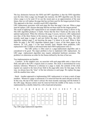
Work: =Available and Finish[i]:=false for i=1,2,3,….., n.
2. Find an I such that both
a. Finish[i]=false
b. Need i Work.
If no such I exists, go to step 4.
3. Work: =Work + Allocation;
Finish[i]: =true
Go to step 2.
4. If Finish[i] = true for all I, then the system is in a safe state.
This algorithm may require an order of m x n operations to decide whether a state is safe.
Resource-Request Algorithm
Let Request i be the request vector for process Pi. If requesti[j] = k, then process pi wants
k instances of resource type Rj. When a request for resources is made by process Pi, the
following actions are taken:
1. If Requesti < Needi, go to step 2. Otherwise , raise an error condition, since the
process has exceeded its maximum claim.
2. If Requesti< Available, go to step 3. Otherwise, Pi must wait, since the resources
are not available.
3. Have the system pretend to have allocated the requested resources to process Pi
by modifying the state as follows:
Available: = Available – Requesti;
Allocationi :=Allocationi + Requesti;
Needi := Needi – Requesti;
If the resulting resource-allocation state is safe, the transaction is completed and process
Pi is allocated its resources. However, if the new state is unsafe, then Pi must wait for
Request and the old resource-allocation state is restored.
41

42. DEADLOCK DETECTION
The graphs (DRAG) provide good help in doing this, as we have seen. However,
normally, a realistic DRAG is not as straight forward as a DRAG between two processes
(P1, P2) and two resources (R1 and R2) as depicted. In reality, there could be a number
of resource types such as printers, plotters, tapes, and so on. For instance, the system
could have two identical printers, and the operating system must be told about it at the
time of printers when requested. The complexity arises due to the fact that allocation to a
process is made of a specific resource by the operating system, depending upon the
availability, but the process normally makes the request to the operating system for only a
resource type. A very large number of processes can make this DRAG look more
complex and the deadlock detection more time consuming.
We will denote multiple instances of the same resource type by means of multiple
symbols within the square. For example, consider the DRAG shown in figure.
Figure: multiple resource for a type
P
1
R1 ( )R10 ( )R20 R2
( )R11
P
2
R1 is a resource type – say, a tape drive of a certain kind, and let us assume that there are
two tape drivers R10 and R11 of the same kind known to the system. R2 may be a of a
certain type there may be only one of that type available in the system – say, R20. In fig,
R10 is allocated to P1. P1 is waiting for R20. R20 is allocated to P2. Now comes the
question of last in the diagram. Let us assume that R11 is free and P2 wants it. In this
case, P2 can actually grab R11. And if it does so, an arrow will be actually drawn from
R11 to P2 as shown in Fig. If you traverse from a node, following the arrows, you would
not arrive at the starting node. This violates the rules for a circular wait. Therefore, even
if it gives an impression of a deadlock at first sight, it is NOT a deadlock situation.
P
1
R1 ( )R10 ( )R20 R2
( )R11
P
2
Figure: no deadlock situation.
42

43. Therefore, P2 in this case need not wait for R11. It can go to completion. The point is that
the visual illusion of the cycle should not deceive us. It is not a circular wait condition. If
R11 however, is also not free and is already grabbed by, say P1, it can lead to a deadlock
if P2 requests for R1.
The operating system, in the case, could do the following to detect a deadlock:
(i) Number all process as P0, P1 ….PN.
(ii) Number each resource separately – using a meaningful coding scheme. For
instance, the first character could always be “R” denoting a resource. The
second character could denote the resource type (0=tape, 1=printer, etc.) and
the third character could denote the resource number or an instance within the
type, e.g. R00, R01, R02,…..could be different tape drivers of the same type;
R10, R11, R12, …….
(iii) Maintain two tables as shown in fig. One is a resource wise table giving ,
for each resource, its type, allocation status, the process to which it is
allocated and the processes that are waiting for it.
Another table is a process wise table, giving for each process, the
resources held by it and the resources it is waiting for. This is normally held along
with PCB. Logically, it is a part of PCB, but an operating system could choose to
maintain it in a separate table linked to the PCB for that process. The operating
system could use this information to detect any deadlock, as we shall see later.
(iv) Whenever a process requests the operating system for a resource, the
request is obviously for a resource belonging to resource type. The user would
not really care which one is exactly allocated (if he did, a new resource type
should have been created). The operating system then goes through the
resource wise table to see if there is any free resource of that type. This also
will necessitate updating of both tables.
When a process releases a resource, again both tables will be updated
accordingly.
(v) At any time, the operating system can use these tables to detect a circular wait
or a deadlock. Typically, whenever a resource is demanded by a process,
before actually allocating it, the operating system could use this algorithm to
see whether the allocation can potentially lead to a deadlock or not.
The working is as follows:
(a) Go through the resource wise table entries one by one (e.g. R00, R01 …etc.),
each time storing the resource numbers processed. This is useful in detecting
a circular wait, i.e. in finding out whether we have reached the same node
again or not.
(b) Ignore entries for free resources.
43

44. (c) For each of the entries, access the process to which the resource is allocated.
In the case, store the numbers R01 and P1 in separate lists called resource list
and process list respectively.
(d) Access the entry in the process wise table for that process obtained in step (c)
(P1 in this case).
(e) Access one by one the resources this process (P1) is waiting for. For example,
P1 is waiting for resource R20. Check if this is the same as the one already
encountered i.e. if R20 Is the same as R01 stored in step (c). In short, check
if circular wait is already encountered. If yes, the deadlock is detected. If no,
store this resource (e.g R20) in the resource list. This list will now contain
R01 and R20. The process list still contains only P1. Whether there is any
other resource apart from R20 that process P1 is waiting for. If there is any,
this procedure will have to be repeated. In this example, there is no such
resource. Therefore, the operating system goes to the next step (f).
(f) Access the next entry in the resource list maintained in step (e). This entry is
R20. Now access the resource wise table for R20 to find that R20 is allocated
to P5.
(g) Check if this process (i.e. P5) is the one already encountered in the process
list maintained in step (e). If it is the same, a deadlock is confirmed. In this
case, P5 is not the same as P1. So only store P5 after P1 in the process list and
proceed. The process list now contains P1 and P5. The resource list is still
R01, R20 as in step (e). After this, the operating system will have to choose
R10 and R23, as they are the resources process P5 is waiting for. It finds that
R10 is allocated to P1 already existed in the process list. Hence, a deadlock
(P1←R20←P5←R10←P1) has been detected.
Therefore, the operating system will have to maintain two lists – one list
of resources already encountered and a separate list of all the waiting
processes already encountered. Any time the operating system list while going
through the algorithm, the deadlock is confirmed.
(h) If a deadlock is not confirmed, continue this procedure for all the
permutations and combinations e.g for all the resources that a process is
waiting for and then for each of these resources, the processes to which they
are allocated. This procedure has to be repeated until both the lists are
exhausted one by one. If all the paths lead to resources which are free and
allocable, there is no deadlock. If all the paths make the operating system
repeatedly got through same process or resource, it is a deadlock situation.
Having finished one row, go to the next one and repeat this procedure for all the rows
where the status is NOT=free.
44

45. PROCESS SYNCHRONIZATION
A system consists on n processes { P0,P1,….,Pn-1}. Each process has a segment of code
called a critical section, in which the process may be changing common variables,
updating a table, writing a file and so on. Each process must request permission to enter
its critical section. The section of code implementing this request is the entry section.
The critical section may be followed by an exit section. The remaining code is the
remainder section.
Fig. General structure of a typical process Pi.
do{
entry section
critical section
exit section
remainder section
} while(1);
A solution to the critical section problem must satisfy the following requirements:
1. Mutual Exclusion: If process Pi is executing in its critical section, then no other
processes can be executing in their critical sections.
2.Progress: If no process is executing in its critical section and some process wish to
enter their critical sections, then only that process not in the remainder section can
enter the critical section.
3. Bounded waiting: There exists a bound on the number of times that other
processes are allowed to enter their critical sections after a process has made a request
to its critical section.
Two Process Solutions:
I. Algorithm 1:
do{
45

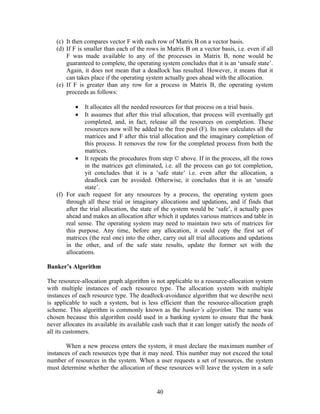
46. while (turn !=j);
critical section
turn = j;
remainder section
} while (1);
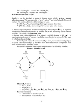
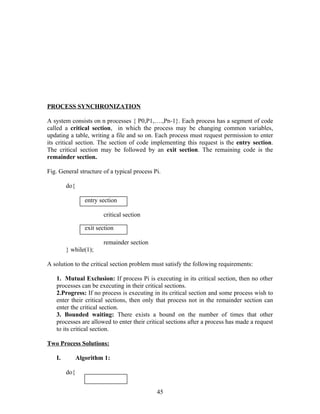
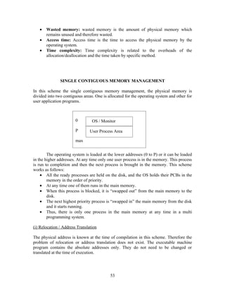
Fig. The structure of process Pi in algorithm 1.
The two processes P0, P1 share the common integer variable turn = 0 or 1. If turn == i,
then process Pi is allowed to execute in its critical section. The structure of Pi is shown in
fig. This solution ensures that only one process at a time can be in its critical section. But
it does not satisfy the progress requirement.
II. Algorithm 2
do{
flag[i] = true;
while (flag[j]);
Critical section
flag[i] = false;
Remainder section
{ while(1);
The remedy to algorithm 1 is we can replace the variable turn with the following array:
Boolean flag[2];
The elements of the array are initialized to false. If flag[i] is true, this value indicates that
Pi is ready to enter the critical section. The structure of Pi is shown in figure.
In this algorithm, process Pi first sets flag[i] to be true, signaling that it is ready to
enter its critical section. Then Pi checks to verify that process Pj is not also ready to enter
its critical section. If Pj were ready, then Pi would wait until Pj no need to be in critical
section. Then Pi will enter critical section and on exiting the critical section, Pi wouls set
flag[i] to be false, allowing the other process to enter its critical section.
In this mutual exclusion is satisfied. But progress is not satisfied. Consider the
following execution:
To: Po sets flag[0] = true
T1: P1 sets flag[1] = true
During time To the process Po is executed and a timing interrupt occurs after To is
executed, and the CPU switches from one process to another.
III. Algorithm 3:
46

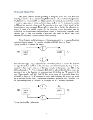
47. By combining the key ideas of algorithm 1 and 2 we obtain the correct solution to the
critical section problem where all the three requirements is met.
The processes share the two variables:
Boolean flag[2];
int turn;
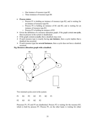
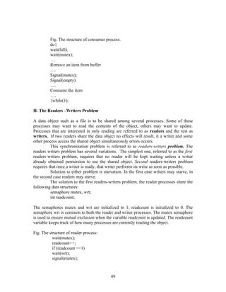
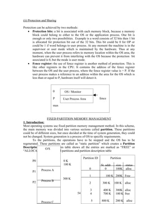
Fig. The structure of process Pi in algorithm 3.
do{
flag[i] = true;
turn = j;
while (flag[j] && turn == j);
critical section
flag[i] = false;
remainder section
} while (1);
Initially flag[o] = flag[1] = false, and the value of turn = 0 or 1.
To enter the critical section, process Pi first sets flag[i]=true and sets turn = j value(1). So
that the pother process wishes to enter the critical section can enter. If both process try to
enter at the same time then value of turn decides which of the two process to enter.
To proves solution is correct show:
1. Mutual exclusion is preserved
2. The progress requirement is satisfied
3. The bounded waiting requirement is met.
To prove property 1:
Pi enters its critical section only is either flag[j] ==false or turn==i. At the time,
flag[j]==true, and turn ==j, until this condition persist as long as Pj is in its critical
section, the result is mutual exclusion is followed.
To prove property 2:
The Process Pi can be prevented from entering the critical section when the condition
flag[j] ==true and turn==j;
If Pj is not ready to enter the critical section , then flag[j] == false and Pi an enter
the critical section.
If Pj has set flag[j] ==true and is and executing in the while loop then either
turn==I or turn==j; If turn==I then Pi will enter the critical section. If turn==j, then Pj
47

48. will enter the critical section. When Pj exists the critical section it will reset the
flag[j]==false allowing Pi to enter the critical section.
If Pj resets flag[j] == true then it must also set turn ==i. Thus, since Pi does not
change the value of the variable turn while executing the while statement, Pi will enter
the critical section(progress) which after at most one entry by Pj(bounded waiting).
CLASSIC PROBLEMS OF SYNCHRONIZATION
I. Bounded Buffer Problem:
This illustrates the concept of cooperating processes, consider the producer and
consumer problem. A producer process produces information that is consumed by a
consumer. Example, a print program produces characters that is consumed by the printer
device. We must have available buffer of items that can be filled by the producer and
emptied by the consumer. A producer can produce one item while the consumer is
consuming another item. The producer and the consumer must be synchronized so that
the consumer does not try to consume n item that has not yet been produced.
In unbounded buffer produce4r consumer problems has no problem on the limit
on the size of the buffer. The consumer have to wait for new items but the producer can
always produce new items.
In bounded buffer producer consumer problem assumes fixed buffer size. In this
case if consumer must wait if the buffer is empty, and the producer must wait if the buffer
is full.
In the bounded buffer problem , we assume the pool consists of n buffers, each
capable of holding one item. The mutex semaphore provides mutual exclusion for access
to the buffer pool and is initialized to the value 1. The empty and full semaphores count
the number of empty and full buffers. The semaphore empty is initialized to value n, and
full initialized to the value 0.
Fig. The structure of the producer process.
do{
….
Produce an item
….
wait(empty);
wait(mutex);
….
add to buffer
….
signal(mutex);
signal(full);
}while(1);
48

49. Fig. The structure of consumer process.
do{
wait(full);
wait(mutex);
….
Remove an item from buffer
….
Signal(mutex);
Signal(empty)
….
Consume the item
….
}while(1);
II. The Readers –Writers Problem
A data object such as a file is to be shared among several processes. Some of these
processes may want to read the contents of the object, others may want to update.
Processes that are interested in only reading are referred to as readers and the rest as
writers. If two readers share the data object no effects will result, it a writer and some
other process access the shared object simultaneously errors occurs.
This synchronization problem is referred to as readers-writers problem. The
readers writers problem has several variations. The simplest one, referred to as the first
readers-writers problem, requires that no reader will be kept waiting unless a writer
already obtained permission to use the shared object. Second readers-writers problem
requires that once a writer is ready, that writer performs its write as soon as possible.
Solution to either problem is starvation. In the first case writers may starve, in
the second case readers may starve.
The solution to the first readers-writers problem, the reader processes share the
following data structures:
semaphore mutex, wrt;
int readcount;
The semaphores mutex and wrt are initialized to 1; readcount is initialized to 0. The
semaphore wrt is common to both the reader and writer processes. The mutex semaphore
is used to ensure mutual exclusion when the variable readcount is updated. The readcount
variable keeps track of how many processes are currently reading the object.
Fig. The structure of reader process:
wait(mutex);
readcount++;
if (readcount ==1)
wait(wrt);
signal(mutex);
49

50. …
reading is performed
…
wait(mutex);
readcount --;
if(readcount ==0)
signal(wrt);
signal(mutex);
Fig. The structure of a writer process:
wait(wrt);
…
writing is performed
…
signal(wrt);
III. The Dining-Philosophers Problem:
Consider five philosophers who spend their lives thinking and eating. The philosophers
share a common circular table surrounded by five chairs each for the five philosophers. In
the center of the table is a bowl of rice, and the table is laid with five single chopsticks.
When a philosopher thinks, she does not interact with her colleagues. From time to time,
a philosopher gets hungry and tries to pick up the two chopsticks that are closest to her. A
philosopher may pick up only one chopstick at a time. She cannot pick up a chopstick
that is already in the hand of a neighbor. When a hungry philosopher has both her
chopsticks at the same time, she eats without releasing her chopsticks. When she is
finished eating, she puts down both of her chopsticks and starts thinking again.
The dining philosopher is a simple representation of the need to allocate
several resources among several processes in a deadlock and starvation free manner. One
simple solution is to represent each chopstick by a semaphore. A philosopher tries to grab
the chopstick by executing a wait operation on that semaphore. She releases her
chopsticks by executing the signal operation on appropriate semaphores. Thus the shared
data are:
Semaphore chopstick[5];
Where all the elements of chopstick are initialized to 1.
do{
wait(chopstick[I]);
wait(chopstick[(I+1)%5];
…
eat
…
signal(chopstick[I]);
signal(chopstick[(I+1)]%5);
…
think
50

51. …
}while(1);
This solution guarantees that no two neighbors are eating simultaneously, it must be
rejected because it has the possibility of creating a deadlock. Suppose that all five
philosophers become hungry simultaneously, and each grabs her left chopstick. All the
elements of chopstick will now be equal to 0. When each philosopher tries to grab her
right chopstick, she will be delayed forever.
Several remedies to deadlock problem are:
• Allow at most four philosophers to be sitting simultaneously at the table.
• Allow a philosopher to pick up her chopsticks only if both chopsticks are
available.
• Use asymmetric solution: an odd philosopher picks up first her left chopstick and
then her right chopstick, whereas an even philosopher picks up her right and then
her left chopstick.
51

52. UNIT – 4
MEMORY MANAGEMENT
The systems can be divided into two major parts “Contiguous” and “Non Contiguous”
memory management.
• Contiguous memory management schemes expect the program to be loaded in
contiguous memory location. It considers of single contiguous memory, fixed
partition memory, and variable partition memory.
• Non contiguous systems remove this problem. They are allowing to program to be
divided into different chunks and to be loaded at different portions of the memory.
It consists of paging, segmentation memory management schemes.
The above schemes will be discussed with the following issues involved in it:
(i) Relocation and Address Translation
Relocation and address translation refers to the problem that arises because , at the time
of compilation, the exactly physical memory locations that a program is going to occupy
at the run time are not known. The compiler executes the machine code assuming that the
program starts fro word 0. At the execution time, the program may need to be relocated to
different location, and all the addresses will need to be changed before execution.
(ii) Protection and Sharing
Protection refers to the prevention o one program from interfering with other programs.
This is true even if only single user process and operating system are both residing in the
main memory.
Sharing is the opposite of protection. In this case multiple processes have to share the
same memory locations. Having 10 copies of the same program in memory for 10
different users is a waste of memory.
(iii) Evaluation
Each of these memory management methods can be judged in terms of efficiency by the
following norms:
52

53. • Wasted memory: wasted memory is the amount of physical memory which
remains unused and therefore wasted.
• Access time: Access time is the time to access the physical memory by the
operating system.
• Time complexity: Time complexity is related to the overheads of the
allocation/deallocation and the time taken by specific method.
SINGLE CONTIGUOUS MEMORY MANAGEMENT
In this scheme the single contiguous memory management, the physical memory is
divided into two contiguous areas. One is allocated for the operating system and other for
user application programs.
0 OS / Monitor
P User Process Area
max
The operating system is loaded at the lower addresses (0 to P) or it can be loaded
in the higher addresses. At any time only one user process is in the memory. This process
is run to completion and then the next process is brought in the memory. This scheme
works as follows:
• All the ready processes are held on the disk, and the OS holds their PCBs in the
memory in the order of priority.
• At any time one of them runs in the main memory.
• When this process is blocked, it is “swapped out” from the main memory to the
disk.
• The next highest priority process is “swapped in” the main memory from the disk
and it starts running.
• Thus, there is only one process in the main memory at any time in a multi
programming system.
(i) Relocation / Address Translation
The physical address is known at the time of compilation in this scheme. Therefore the
problem of relocation or address translation does not exist. The executable machine
program contains the absolute addresses only. They do not need to be changed or
translated at the time of execution.
53

54. (ii) Protection and Sharing
Protection can be achieved by two methods:
• Protection bits: a bit is associated with each memory block, because a memory
block could belong to either to the OS or the application process. One bit is
enough or only two possibilities. Example is a word consists of 32 bits then 1 bit
is allocated for protection bit out of the 32 bits. This bit could be 0 for OP or
could be 1 if word belongs to user process. At any moment the machine is in the
supervisor or user mode which is maintained by the hardware. Thus at any
moment, when the user process refers to memory location within the OS area, the
hardware can prevent it from interfering with the OS because the protection bit
associated is 0, but the mode is user mode.
• Fence register: the use of fence register is another method of protection. This is
like other registers in the CPU. It contains the address of the fence register
between the OS and the user process, where the fence register value is = P. If the
user process makes a reference to an address within the area for the OS which is
less than or equal to P, hardware itself will detect it.
0 OS / Monitor
P User Process Area fence
e
max
FIXED PARTITION MEMORY MANAGEMENT
1. Introduction:
Most operating systems use fixed partition memory management method. In this scheme,
the main memory was divided into various sections called partition. These partitions
could be of different sizes, but once decided at the time of system generation, they could
not be changed. System generation is a process of OS to specific requirements.
To the partitions, the operations have to be stopped and the OS has to be
regenerated. These partitions are called as “static partition” which creates a Partition
Description Table(PDT). This table shows all the entries are marked as “FREE” or
O/S
“ALLOCATED” Fig. Fixed partitions and partition description table
Partition ID Partition
P0 0K
100 K St. addr size status
Process A 0 0 100K alloc
P1
1 100 K 200K Free
300 K
P2 Process B
2 300 K 100 K alloc
3 400 K 300K alloc
54 4 700 K 100 K free
Process C 5 800 K 200 K alloc

55. 400 K
P3
700 K
P4
800 K
P5 1000 K
When a partition is to be allocated to a process, the following takes place:
1. Decide which partition is to be brought into the memory next.
2. It finds the size of the program to be loaded
3. It then makes a request to the partition allocation routine of the MM to allocate
the free partition with the appropriate size.
4. It now loads the binary program into the allocated partition.
5. It then makes an entry of the partition ID in the PCB before the PCB is linked to
the chain of the ready processes.
6. The routine in the MM now marks the status of the partition as “allocated”
2. Allocation Algorithms:
The OS maintains and uses the PDT as in figure. In this fig. Partition 0 is occupied by
OS and is thus unallocable. The “FREE” partitions are only 1 and 4. Thus if new
process is to be loaded, we have to choose from 1 or 4. The process waiting to be
loaded in the memory are held in a queue by the OS. There are two methods of
maintaining this queue, multiple queues and single queue.
Multiple Queues:
In multiple queues there is one separate queue for each partition. For instance:
queue 0 - will hold processes with size 0-2K
queue 1 - will hold processes with size between 5K and 8K
queue 2 - will hold processes with size between 2K and 5K
When a process wants occupy memory it is added to a proper queue depending upon
the size of the process. Scheduling can be round robin, FIFO or priority. An
advantage of this scheme is that very small process are not loaded in a very larger
partition.
Monitor
Queue0 1K 1K 2K 1K 2K 1K
2K
Queue 1 …….. 6K 7K 6K 8K
8K
Queue 2 …….. 3K 4K 5K 3K
55 5K

56. Fig. Multiple queues.
Single queues:
In the single queue only one queue is maintained of all the ready processes. The order in
which PCBs of ready processes are chained, depends upon the scheduling algorithm. The
PCB contains the process size. A free partition is then found based on either the first, best
or worst fit algorithm.
Monitor
3K 8K 2K 7K
2K
8K
5K
Fig. Single queue
If the PCB at the head of the queue requires memory which is not available now, but
there is a free partition available to fit the process represented by the next PCB in the
queue. Example the partition with size = 5K is free, the highest priority process at the
head of the chain with size =7K cannot be dispatched. The OS then has to find the next
process in the queue which can fit into the 5 K partition. In this case the OS finds the next
process with size=2K can fit well. External fragmentation occurs in this scheme.
Swapping:
Lifting the program from memory and placing it on the disk is called “swapping out”.
To bring the program again from the disk into the main memory is called “swapping in”.
Swapping algorithm has to coordinate amongst information, process and memory
management systems. If the operating system completes the I/O on behal of the blocked
process which was swapped out, it keeps the data read recently in its own buffer. When
the process is swapped in again, the OS moves the data into the I/O area of the process
and then makes the process ‘ready’.
OS has to find a place on the disk for the swapped out process. There
are two approaches for this:
• to create a separate swap file for each process. This method is very flexible, but
can be very inefficient due to the increased number of files and directory entries.
56

57. • To keep a common swap file on the disk and the note the location of each
swapped out process within that file. In this scheme estimate the swap file size. If
a smaller area is reserved for this file, the OS may not be able to swap out
processes beyond a certain limit.
Relocation and Address Translation:
Static Relocation and AT: This is performed before or during the loading of the
program in the memory, by the relocating linker or relocating loader. The compiler
compiles the program assuming the program is to be loaded in the main memory at the
starting address0. The relocating linker/loader goes through each instruction and changes
the addresses in each instruction of the program before it is loaded and executed.
Starting address of the partition
Relocated program
Compiled Relocating with changed
program linker/ loader addresses
Fig. Static relocation
Dynamic relocation:
Dynamic relocation is used at the run time for each instruction. It is normally done by a
special piece of hardware. It is faster but expensive called as “base register”. This
register contains the value of relocation. In this case the compiled program is loaded at a
starting memory location different than 0 without any change to any instruction in the
program. Example instruction “LDA 500” actually loaded at some memory locations
between 1000 to 1500. The address 500 in this instruction is invalid as it is the logical
address. Hence the address in the instruction must be changed to physical address during
run time.
Normally any instruction such as “LDA 500” when executed is fetched to
instruction register (IR). Where the address portion is separated and sent to memory
address register (MAR). Before this is done the base register value 1000 is added to it and
only the resulting address 1500 finally goes to MAR. 1500 refers to the physical address.
Base register
1000
IR MAR
500 + 1500 LDA
500
Virtual physical
Address address
57
Physical memory

58. Fig. Dynamic relocation
Protection and sharing:
There are two approaches in this scheme:
• Protection bits
• Limit register
Protection bits;
The idea of single user system except that 1 bit not sufficient for protection hence uses 4
bits. Example if there are 16 user processes running in 16 partitions. If the word length is
32, 4 bits allocated for protection bits 4/32= 1/8 or 12.5% increase in overheads. The
IBM series of computers divide the computer memory into 2 KB blocks and reserved 4
protection bits called “key” But this resulted in memory wastage or internal
fragmentation. Assume that the block size is 2 KB, and the process size is 10KB + 1
byte, if two are the partitions are of size 10 KB and 12KB, the OS with 12 KB has to be
allocated as 10 KB will not be enough. So this leads to memory wastage called internal
fragmentation.
Protection keys PSW
2K Partition 0 0000 0000
4K Partition 1 0001 0001
0001
Partition 2 0010 0010
8K 0010
0010
0010
2K Partition 3 0011 0011
Partition 15 1111 1111
4K
1111
All the blocks associated with a partition allocated to a process are given the same
key value in this scheme. If the number of partitions are 16, there can be a maximum 16
58

59. user processes at any moment in the main memory. Therefore a 4 bit key value ranging
from 0000 to 1111 is used.
Limit register:
Another method of providing protection is by using a limit register, which ensures that
the virtual address present in the original instruction, moved into IR before any
relocation/Address translation, is within the bounds of the process address space. If the
program size is 1000, the virtual addresses would range from 0 to 999. In this case the
limit register would be set to 999. Every logical or virtual address will be checked to
ensure it is less than or equal to 999 and only then added to the base register. If it is not
within the bounds, the hardware itself will generate an error message and the process will
be aborted.
Sharing:
Sharing process is a serious problem in fixed partitions, because it might compromise on
protection.
• One approach is to keep copies of the sharable data in all partitions where
required. But it is wasteful, and the same pieces of data are updated differently in
two different partitions.
• Other way is to keep all the sharable code and data in one partition, and with
either change to base/limit registers allowing controlled access to this partition
even from outside by another process.
Evaluation:
1. Wasted memory:
If a partition of size 100K is allocated to a process of size 60K, then the 40K
space of that partition is wasted and cannot be allocated to any other process. This is
called internal fragmentation. But it may happen that two free partitions of size 20K
and 40K are available and a process of 50K is to be accommodated. In this case both
the available partitions cannot be allocated to that process, because it will violate our
assumption of contiguous memory. And hence the space is wasted. This is called as
external fragmentation.
2. Access Time:
The access time is not very high due to the assistance of special hardware. The
translation from virtual to physical address is done by the hardware itself and hence
rapid access.
3. Time Complexity:
Time complexity is very low, because allocation/deallocation routines are simple,
as the partitions are fixed.
59

60. VARIABLE PARTITION
Variable partitions came to overcome the problems of fixed partition. The number of
partitions and their sizes can vary. They are not defined at the time of generation. At any
time the partition can be free or allocated. The only difference between fixed and variable
partition the starting address if the variable partitions is unknown.
The eight states of the memory allocations in the figure correspond to the eight
events which are given below:
(i) The OS is loaded in the memory. All the rst of the memoery is free.
(ii) A program P1 is loaded in memory and it starts executing
(iii) A program P2 is loaded in the memory and it starts executing
(iv) A program P3 is loaded in the memory and it starts executing
(v) The process P1 is blocked. After a while a new high priority program P4
wants to occupy the memory. The existing free space is less than the size of
P4. Assume that P4 is smaller that P1 but bigger than the free area available
at the bottom.P1 is swapped out and now two chunks of free space is
available.
(vi) P4 is now loaded in the memory and it starts executing. P4 is loaded in the
same space where P1 was loaded.
(vii) P2 terminates. Only P4 and P3 continue. The free are at the top and the one
released by P2 can now be joined together. There is now a large free space in
the middle, in addition to a free chunk at the bottom.
(viii) P1 is swapped in as the OS has completed the I/O on its behalf and the data is
already in the buffer of the OS. Also the free space in the middle is sufficient
to hold P1 now. Another process P5 is also loaded in the memory. Only little
free space is left.
os os
(i) (ii) (iii) (iv) (v) (vi) (vii)
(viii)
60

61. Allocation Algorithm
The basic information needed to allocate and deallocate is the same as given in the PDT
in fixed partition. The same information is normally kept as bitmaps or linked lists.
In bitmap method, the OS maintains 1 bit for each chunk denoting if it is allocated (1)
and for free(0).
In linked list we create a record for each variable partition. Each record maintains
information such as:
• Allocated/Free (F=free, A=allocated)
• Starting chunk number
• Number of chunks
• Pointer to the next entry
In this scheme of variable partitions, when a chunk is allocated to a process or a process
terminates, thereby freeing a number of chunks, the bit map or the linked list is updated .
Merits and Demerits for both approaches:
Bitmaps are very fast for deallocation. But slow for allocations. For instance if the
process terminates, the OS just carries out the following steps:
• Access the PCB of the terminated process
• Find out the starting chunk number and the number of chunks allocated to that
process.
• Access the corresponding bits for those chunks in the bit map and set them to 0.
0 4 7 9 14 15 17 20 24 25
28
P1 P2 P3 P4 P5 P6
(a) Memory Allocation
00001110011111011000111100111
(b) Bitmap
F 0 4 A 4 3 F 7 2 A 9 5
F 14 1 A 15 2 F 17 3 A 20 4
F 24 2 A 26 1 A 27 2 *
61

62. (c) Linked List
Compaction:
This technique shifts the necessary process images to bring the free chunks to adjacent
position. There could be different ways to achieve compaction. For instance, in the
method shown in fig. B the OS has to move P3 (size=400) and P4(size=800). Hence the
total movement is 1200. Fig c, only P4 (size=800) is moved in the free chunk of 800
available (1201-2000). Hence the total movement is only 800. In fig d. only P3
(size=400) in the free chunk of contiguous chunk is in the middle in this case. The
method d is best.
When ever a process terminates, the OS would do the following:
(i) Free that memory
(ii) Coalesce if necessary
(iii) Check if there is another free space which is not contiguous and if yes do
compaction process
(iv) Create a new bitmap/linked list as per the new memory allocations.
(v) Store the starting address of the partitions in the PCBs of the corresponding
processes.
Fig: Compaction: different possibilities.
Swapping:
62

63. The swapping considerations are almost identical to those of fixed partitions.
Relocation and Address Translation:
This is same as in fixed partitions. This depends upon the base register which is stored for
calculating the physical address from the logical address.
Protection and Sharing:
Protection is achieved with the help of the limit register. Before calculating the physical
address, the virtual address is checked to ensure that it is equal to or less than the limit
register.
Sharing is possible only to a limited extent by suing “Overlapping partitions” as in fig.
Process Base Limit 3000
A 3000 4000
A A
B 6000 3000 6000
7000 A, B shared
B
B
9000
Fig. Overlapping Partitions
Evaluation:
1. Wasted memory:
2. Access Time:
3. Time Complexity:
SWAPPING
A process needs to be in a memory to be executed. A process, can be swapped
temporarily out of memory to a backing store, and then brought back into memory for
continued execution. For example, assume a multiprogramming environment with a
round robin CPU scheduling algorithm. When a time quantum expires, the memory
manager will start to swap out the process that just finished, and to swap in another
process to the memory space that has been freed. In meantime the CPU scheduler will
allocate a time slice to some other process in memory. When each process finishes its
63

64. quantum, it will be swapped with another process. The memory manager can swap
processes.
Another variant of swapping policy is used for priority based scheduling
algorithms. If a higher priority process arrives and wants service, the memory manager
can swap out the lower priority process so that it can load and execute the higher priority
process. When the higher priority process finishes the lower priority process can be
swapped back and continued. This is also called as roll in and roll out.
Normally a process that is swapped out will be swapped back into the same
memory space that it occupied previously. This restriction is dictated by the method of
address binding. If binding is done at load time, then the process cannot be moved to
different locations. If execution time binding is being used then a process can be swapped
into a different memory space.
Swapping requires a backing store. The backing store is commonly fast disk. It
must be large enough to accommodate copies of all memory for all users, and it must
provide direct access to these memory. The system manages a ready queue consisting of
all processes whose memory are on the backing store or in memory and are ready to run.
When the CPU scheduler decides to execute a process, it calls the dispatcher.
The context switch time in such a swapping is high. For, example of context
switch assume the process is of size 1MB and the backing store is a standard hard disk
with a transfer rate of 5 MB per second. The actual transfer of 1 MB process to or from
memory takes:
1000 KB / 5000 KB per second = 1 / 5 second = 200 milliseconds.
Swapping is constrained by other factors as well:
If we want to swap a process, we must be sure that it is completely idle. Particularly is I/
O operation is pending. A process may be waiting for an I/O operation when we want to
swap that process to free up its memory then swapping is not done. Assume that the I/O
operation was queued because the device was busy. Then if we were to swap out process
P1 and swap P2, the I/O operation might then attempt to use the memory which now
belongs to P2.
CONTIGUOUS MEMORY ALLOCATION
The main memory is divided into two partitions: one for the resident of the OS and one
for the user processes. The OS may be in either the low or high memory. In contiguous
memory allocation, each process is contained in a single contiguous section of memory.
SEGMENTATION
Segmentation is a memory-management scheme that supports this user view of memory.
A logical address space is a collection of segments. Each segment has a name and a
length. The addresses specify both the segment name and the offset within the segment.
The user there specifies each address by two quantities:
64

65. • Segment name
• Offset
Segments are numbered and referred as segment number, rather than by a segment name.
Thus a logical address consists of two tuples:
<segment number, offset>
The user program is compiled and the compiler automatically constructs segments
reflecting the input program.
Hardware:
User refers to program by a two dimensional address, the actual physical memory is one
dimensional sequence of bytes. So the two dimensional user defined address is mapped
into two physical addresses. This mapping is affected by a segment table. Each entry of
the segment table has a segment base and a segment limit. The segment base contains
the starting physical address where the segment resides in memory, whereas the segment
limit specifies the length of the segment.
Use of segment table is shown in the figure. A logical address consists of two parts: a
segment number, s and the offset into that segment, d. The segment number is used as
an index into the segment table. The offset d of logical address must be between 0 and the
segment limit. If not then we trap a addressing error. If this offset is legal, it is added to
the segment base to produce the address in physical memory of the desire byte.
s
Limit base
Segment table physical memory
CPU S d
yes
< +
no
trap addressing error
Fig. Segmentation hardware
65

66. As an example, consider the situation as in below fig. We have five segments numbered
from 0 through 4. The segments are stored in physical memory as shown. The segment
table has a separate entry for each segment, giving the beginning address of the segment
in physical memory and the length of the segment(limit). For example, segment 2 is 400
bytes long and begins at location 4300. Thus a reference to byte 53 of segment 2 is
mapped onto location 4300+53 = 4353. A reference to segment 3, byte 852 is mapped to
3200 (the base of segment 3) + 852 = 4052. A reference to byte 1222 of segment 0 would
result in a trap to the OS, as this segment is only 1000 bytes long.
stack
subro
1400
utine
Segment3 Segment 0
Symbol 2400
Segment 0 table
Segment 1 3200
sqrt Segment 4 Segment 3
Main 4300
Limit base
program
0 4700 Segment 2
1000 1400
1
Segment 2 400 6300 Segment 4
2
400 4300 5700
1100 3200
logical address space 3 6300
1000 4700
4 6700
Segment 1
physical address
Protection and Sharing:
Advantage of segmentation is protection with the segments. Some of the segment are
instructions and some are data. The memory mapping hardware will check the protection
bits associated with each segment table entry to prevent illegal accesses to memory, such
as attempts to write into a read only segment, or to use an execute only segment as data.
Another advantage of segmentation involves the sharing of the code or data.
Each process has a segment table associated with it, which the dispatcher uses to define
the hardware segment table when this process is given the CPU. Segments are shared
when entries in the segment tables of two different processes point to same physical
location as in below figure.
The sharing occurs at the segment level. Thus any information can be shared if
it is defined to be a segment. Several segments can be shared.
For example, consider the text editor in a time sharing system. The editor consists of
many segments. These segments can be shared among all the users, rather than n copies
of the editor for each user.
Even parts of programs can be shared if they are declared sharable, Read only
segments.
66

67. editor 43062
Limit base
Segment 0 0 25286 43062 Editor
1 4425 68348
Data 1 72773 Data 1
Segment 1 segment table process p1
Logical memory process P1
90003
Limit base Data 2
editor 25286 43062 98553
8850 90003
Segment 0
Segment table process P2 Physical memory
Data 1
Segment 1
Logical memory process P2
Fragmentation:
The long term scheduler must find and allocate memory for all the segments of a user
program. This situation is similar to paging except that the segments are of variable
length; pages are all the same size. Thus, as with the variable-sized partition scheme,
memory allocation is a dynamic storage allocation problem.
Segmentation may then cause external fragmentation, when all blocks of free
memory are too small to accommodate a segment. In this case, the process may simply
have to wait until more memory becomes available, or until compaction creates a larger
hole. Because segmentation is done by its nature a dynamic relocation algorithm, we can
compact memory whenever we want.
67

68. VIRTUAL MEMORY
Virtual memory is the separation of user logical memory from physical memory. This
separation allows an extremely large virtual memory to be provided for programmers
when only a smaller physical memory is available. Virtual memory also allows files and
memory to be shared by several different processes through page sharing.
Virtual memory is commonly implemented by demand paging. It can
also be implemented in segmentation system. Demand segmentation can also be used to
provide virtual memory.
DEMAND PAGING
A demand paging system is similar to a paging system with swapping. Processes reside
on secondary memory. When a process is to be executed, it is swapped into the memory.
Rather than swapping the entire process a lazy swapper is used. The lazy swapper
never swaps a page into memory unless that page will be needed.
Basic Concepts:
When a process is to be swapped in, the pager guesses which pages will be used before
the process is swapped out again. Instead of swapping in a whole process, the pager
brings only those necessary pages into memory. Thus it avoids reading into memory
pages that will not be used, decreasing the swap time and the amount of physical memory
needed.
Fig: Transfer of paged memory to contiguous disk space.
Swap out
Program A 0 1 2 3
4 5 6 7
8 9 10 11
Program B swap in 12 13 14 15
16 17 18 19
20 21 22 23
68

69. Main memory
We must now distinguish those pages which are on the disk and those on memory. There
is a valid – invalid bit, valid bit indicates the pages are in the memory, invalid bits
indicate the pages are not on memory they are on the disk.
Fig: Page table when some pages are not in main memory.
0
0 A
1 B 1
2 C 0 4 v 2
3 1 I 3
D 6 v 4 A
4 E 2
5 F 3 I 5 A
4 I 6 C
6 G 5 9 v 7
7 H
6 I 8
logical memory 7 i 9 F
10
page table 11
12
13
14
physical memory
Access to a page marked invalid causes a page-fault trap.
The procedure for handling this page fault is:
1. We check an internal table to determine whether the reference was a valid or a
invalid memory access.
2. If the reference was invalid, we terminate the process. It is was valid, but we have
not yet brought in that page
3. We find a free frame
4. We schedule a disk operation to read the desired page into the newly allocated
frame.
5. When the disk read is complete, we modify the internal table kept with the
process and the page table to indicate that the page is now in memory.
6. We restart the instruction that was interrupted by the illegal address trap.
69

70. 3. page is on backing store
Operating system
1.reference 2. trap
Load M i
6 restart
Page table
instr
Free frame
5 reset page
table 4 bring in missing page
Fig. Steps in handling a page fault
PAGE REPLACEMENT
Page replacement takes the following approach. If no frames is free, we find one that is
not currently being used and free it. We can free a frame by writing its contents to swap,
and changing the page table. We can now use the freed frame to hold the page for which
the process faulted. We modify the page fault service routine to include page
replacement.:
1. Find the location of the desired page on the disk.
2. Find a free frame:
a. If there is a free frame, use it.
b. If there is no free frame, use a page replacement algorithm to select a
victim frame.
c. Write the victim page to the disk; change the page and frame tables
accordingly.
3. Read the desired page into the free frame; change the page and frame tables.
4. Restart the user process.
victim
70

71. frame valid-invalid bit
1. swap out
2. change to invalid victim page
0 i
f
f v 4. reset page
table for new page 3. swap desired
page in
page table
physical memory
Fig: page replacement
I. FIFO Page Replacement
The simplest page-replacement algorithm is a FIFO algorithm. A FIFO replacement
algorithm associates with each page the time when that page was brought into memory.
When a page must be replaced, the oldest page is chosen. We replace the page at the head
of the queue. When a page is brought into memory, we insert it at the tail of the queue.
For our example reference string, our three frames are initially empty. The first
three reference (7, 0, 1) cause page faults, and are brought into these empty frames. The
next reference (2) replaces page 7, because page 7 was brought in first. Since 0 is the next
reference and 0 is already in memory, we have no fault for this reference. The first
references to 3 results in page 0 being replaced , since it was the first of the three pages in
memory (0, 1, and 2) to be brought in Because of this replacement, the next reference, to
0 will fault. Page 1 is then replaced by page 0. Every time a fault occurs, we show which
pages are in our three frames. There are 15 faults altogether.
The FIFO page –replacement algorithm is easy to understand and program.
However, its performance is not always good. The page replaced may be an initialization
module that was used a long time ago and is no longer needed. On other hand ,it could
contain a heavily used variable that was initialized early and is in constant use.
To illustrate the problems that are possible with a FIFO page replacement
algorithm, we consider the reference string.
1,2,3,4,1,2,5,1,2,3,4,5.
reference string
71

72. 7 0 1 2 0 3 0 4 2 3 0 3 2 1 2 0 1 7 0 1
Most unexpected result is known as belady’s anomaly: for some page-replacement
algorithms, the page-fault rate may increase as the number of allocates frames increases.
II. Optimal page replacement
One result of the discovery of belady’s anomaly was the
search for an optimal page-replacement algorithm. An optimal page-replacement
algorithm has the lowest page-fault rate of all algorithms, and will never suffer from
belady’s anomaly. Such an algorithm does exist, and has been called OPT or MIN. It is
simply
Replace the page that will not be used
for the longest period of time.
Use of the page -replacement algorithm guarantees the lowest possible page fault rate for
a fixed number of frames.
For example, an our sample reference string, optimal page-replacement algorithm
would yield nine page faults, as shown in the fig. The first three reference cause faults
that fill the three empty frames. The reference to page 2 replaces page 7, because 7 will
not be used until reference 18, whereas page 0 will be used at 5 and page 1 at 14. The
reference to page three replaces page 1, as page 1 will be the last of the three pages in the
memory to be referenced again. With only 9 page faults, optimal replacement is much
better than a FIFO algorithm, which had 15 faults
7 0 1 2 0 3 0 4 2 3 0 3 2 1 2 0 1 7 0 1
Fig. Optimal Page Replacement
III. LRU page replacement
72

73. The key distinction between the FIFO and OPT algorithms is that the FIFO algorithm
uses the time when a page was brought into memory; the OPT algorithm uses the time
when a page is to be used. If we use the recent past as an approximation of the near
future, then we will replace the page that has not been used for the longest period of time.
This approach is the least –recently-used (LRU) algorithm.
LRU replacement associates with each page the time that page’s last use. When a page
must be replace, LRU chooses that page that has not been used for the longest period.
The result of applying LRU replacement to our example reference string is shown in fig.
The LRU algorithm produces 12 faults. Notice that the first 5 faults are the same as the
optimal replacement. When the reference the page 4 occurs, however, LRU replacement
sees that, of the three frames in the memory, page 2 was used least recently. The most
recently used page is page 0, and just before the page 3 was used. Thus, the LRU
algorithm replaces page 2, not knowing the page 2 is about to be used. When it then
faults for page 2, the LRU algorithm replaces page 3 since, of the three pages in the
memory {0, 3,4}, page 3 is the least recently used. Despite these problems, LRU
replacement with 12 faults is still much better then FIFO replacement with 12.
The LRU policy is often used as a page-replacement algorithm and is
considered to be good. The major problem is hoe to implement LRU replacement. An
LRU page –replacement algorithm may require substantial hardware assistance. The
problem is to determine an order for the frames defined by the time of last use.
Two implementation are feasible:
. Counters: In the simplest case, we associate with each page-table entry a time-of-use
field, and add to the CPU a logical clock or counter. The clock is incremented for every
memory reference. Whenever a reference to a page is made, the contents of the clock
register are copied to the time-of-use field in the page-table entry for that page. In this
way, we always have the “time” of the last reference to each page. We replace the page
with the smallest time value.
. Stack: Another approach to implementing LRU replacement is to keep a stack of page
numbers. Whenever a page is referenced, it is removed from the stack and put on the top.
In this way, the top of the stack is always the most recently used page and the bottom is
the LRU page. Because entries must be removed from the middle of the stack, it is best
implemented by a doubly linked list, with a head and tail pointer.
7 0 1 2 0 3 0 4 2 3 0 3 2 1 2 0 1 7 0 1
Fig: LRU page-replacement algorithm.
73

74. IV. Counting-Based Page Replacement
There are many other algorithms that can be used for page replacement. For
example, we could keep a counter of the number of references that have been made to
each page, and develop the following two schemes.
The least frequently used (LFU) page-replacement algorithm requires that the page with
the smallest count be replaced. The reasons for this selection are that an actively used
page should have a large reference count. This algorithm suffers from the situation in
which a page is used heavily during the initial phase of a process, but then is never used
again. Since it was used heavily, it has a large count and remains in memory even though
it is no longer needed. One solution is to shift the counts right by 1 bit at regular intervals,
forming an exponentially decaying average usage count.
The most frequently used (MFU) page-replacement algorithm is based on the
argument that the page with the smallest count was probably just brought in and has yet
to be used.
THRASHING
When page faults occurs again, again, and again. The process continues to fault,
replacing pages for which it then faults and brings back in right away. This high paging
activity is called thrashing. A process is thrashing if it is spending more time paging than
executing.
I. Cause of Thrashing:
Thrashing results in severe performance problems. The OS monitors CPU utilization. If
CPU utilization is too low, we increase the degree of multiprogramming by introducing a
new process to the system. A global page replacement algorithm is used, it replaces
page with no use to the process to which they belong. Now that process enters a new
phase in its execution and needs more frames. It starts faulting and taking frames away
from other processes. These processes need those pages, so they also fault, taking frames
from other processes. These faulting processes must use the paging device to swap pages
in and out.
The scheduler sees the decreasing CPU utilization, and increases the degree of
multiprogramming as a result. The new process tries to get started by taking frames from
running processes, causing more page faults, and a longer queue for the paging device.
The CPU scheduler tries to increase the degree of multiprogramming more. Thrashing
has occurred and memory access time increases. No other work is getting done because
the processes re spending all there time paging.
thrashing
74

75. CPU
utilization
Degree of multiprogramming
Thrashing can be limited by using a local replacement algorithm. With local
replacement, if one process starts thrashing, it cannot take frames from another process. If
processes are thrashing, they will be in the queue for the paging device most of the time.
The average service time for a page fault will increase, due to the longer average queue
for the paging device. Thus, the effective access time will increase even for a process that
is not thrashing.
To Prevent thrashing:
The number of frames each process needs has to be specified. But how to know the
number of frames it “needs”.
There are several techniques: The working – set strategy – starts by looking at how
many frames a process is actually using. This approach defines the locality model of
process execution.
The locality model states that, as a process executes, it moves from locality to
locality. A locality is a set of pages that are actively used together. A program is
generally composed of several different localities, which may overlap.
II. Working – Set Model:
The Working-set model is based on the assumption of locality. This model uses a
parameter ∆, to define the working-set window. The idea is to examine the most recent
∆ page references. The set of pages in the most recent ∆ page references is the working
set . If a page is in the active use, it will be in the working set. If it is no longer being
used, it will drop from the working set ∆ time units after it last reference.
For example, given the sequence of memory references shown in the figure, if ∆ = 10
memory reference, then the working set at time t1 is {1,2,5,6,7}. By time t2, the working
set has changed to {3,4}.
Figure: Working set model.
75

76. …2615777751 623412 3444343444 13234443444...
∆ ∆
t1 t2
WS(t1)={1,2,5,6,7} WS(t2)={3,4}
The most important property of the working set is its size. If we compute the working set
size, WSS, for each process in the system, we can consider
D = Σ WSS I
Where D - is the total demand for frames. Thus process I needs WSSi frames. If the total
demand is greater than the total number of available frames (D>m), thrashing will occur,
because some processes will not have enough frames.
Use of working-set model:
The OS monitors the working set of each process and allocates to that working set
enough frames to provide it with its working set size. If there are enough extra frames,,
another process can be initiated. If the sum of the working-set size increase, exceeding
the total number of available frames, the operating system selects a process to suspend.
The process pages are written out and its frames are reallocated to other processes. The
suspended process can be restarted later.
This working set prevents thrashing while keeping the degree of
multiprogramming as high as possible.
Difficulty of working set model:
The difficulty is keeping track of the working set.
III. Page Fault Frequency:
The working set model is successful and knowledge of the working set can be useful for
preparing but it seems a difficult way to control thrashing. A strategy that uses the page
fault frequency (PFF) takes a more direct approach.
76

77. Increase
number of frames
page Upper bound
fault
rate
Lower bound
Decrease number of frames
Number of frames
Fig: Page – fault frequency
The specific problem to prevent thrashing. Thrashing has a high page-fault rate. Thus, we
want to control the page-fault rate. When it is too high, the process needs more frames. If
the page fault is too low, then process may have too may frames. So establish a lower and
higher bounds on the desire page-fault rate. If the actual page fault rate exceeds the upper
limit, we allocate that process another frame, if the page fault rate falls below the lower
limit, we remove a frame from that process. Thus we an directly measure and control the
page-fault rate to prevent thrashing.
77

78. UNIT V
FILE CONCEPTS
Computers can store information on several different storage medium, such as
magnetic disks, magnetic tapes, and optical disks. Files are non volatile, so the contents
are persistent through power failures and system reboots. A file is a named collection of
related information that is recorded on secondary storage. Data files may be numeric,
alphabetic, alphanumeric, or binary. Files may be free form, such as text files, or may be
formatted rigidly.
A file has a certain defined structure according to its type. A text file is a
sequence of characters organized into lines. A source file is a sequence of subroutines
and functions, each of which is further organized as declarations followed by executable
statements. An object file is a sequence of bytes organized into blocks understandable by
the system linker. An executable file is a series of code sections that the loader can bring
into memory and execute.
File Attributes:
A file is named, for the convenience of its human users and is referred to bny its name. A
name is usually a sting of characters, A file has certain other attributes which vary from
one operating system to another, they are:
• Name: The symbolic file name is the only information kept in human readable
form.
• Identifier: This unique tag, usually a number identifies the file within the file
system; it is the non-human readable name for the file.
• Type: This information is needed for those systems that support different types.
• Location: This information is a pointer to a device and to the location of the file
on the device.
• Size: The current size of the file and the maximum allowed size are included in
this attribute.
• Protection: Access control information determines who can do reading, writing,
executing and so on.
• Time, date, and user identification: This information may be kept for creation,
last modification, and last use. Thee data are useful for protection, security and
usage monitoring.
File Operations:
A file is an abstract data type. To define a file properly, we need to consider the
operations that can be performed on files. The operating system can provide system calls
to create, write, read, reposition, delete and truncate files along with the other basic six
operations are:
78

79. • Creating a file: The two steps in creating file are 1. Space in system file must be
found for the file. 2. an entry for the new file must be made in the directory. The
directory entry records the name of the file and the location in the file system, and
possibly other information.
• Writing a file: to write we specify both the name of the file and the information
to be written to the file. Given the name of the file the system reaches the
directory to find the location of the file. The system must keep the write pointer to
the location in the file where the next write sis to take place. The write pointer
must be update whenever the write occurs.
• Reading a file: To read a file, system call specifies the name of the file and where
the next block of the file should be put. The system needs to keep a read pointer to
the location in the file where the next read is to take place. Once the read has
taken place the read pointer is updated.
• Repositioning within a file: The directory is searched for the appropriate entry,
and the current file position is set to a given value. Repositioning within a file
does not need to involve any actual I/O. This file operation is also known as a file
seeks.
• Deleting a file: To delete a file, we search the directory for the named file.
Having found the associated directory entry, we release all file space so that it can
be reused by other files, and erases the directory entry.
• Truncating a file: The user may want to erase the contents of a file but keep its
attributes. The attributes remain unchanged except for the file length which is
reset to length zero and its file space is released.
File Types:
A common technique for implementing file types is to include the type as part of the file
name. The name is split into two parts – a name and an extension, usually separated by a
period character. The system uses the extension to indicate the type of the file and the
type of operations that can be done on that file. Only files with .com, .exe. .bat extensions
can be executed.
File type Extension Function
Executable Exe, com, bin Read to run machine language program
Object Obj Compiled machine language
Source code C, java pas Source code in various language
Batch Bat Commands to command interpreter
Text Txt, doc Textual data, documents
Word processor wp, tex, doc Various word processor formats
Library Lib, dll Libraries of routines for programmers
Multimedia Mpeg, mov, rm Binary file containing audio or A/V
information
79

80. Access Methods
Files store information. When it is used, this information must be accessed and read into
computer memory. The information in the file can be accessed in several ways.
1. Sequential Access:
The simplest access method is sequential access. Information in the file is processed in
order, one record after the other. The bulk of the operations on a file reads and writes. A
read operation reads the next portion of the file and automatically advances a file pointer
which tracks the I/O location. A write appends to the end of the file and advances to the
end of the newly written material (end of file). Sequential access is based on a tape model
of a file.
Current position
Beginning end
Rewind read or writes
Fig. Sequential access file
2. Direct Access:
Another method is direct access. A file is made up of fixed length logical records that
allow programs to read and write records rapidly in no particular order. The direct access
method is based on a disk model of a file, since disks allow random access to any file
block. A direct access file allows arbitrary blocks to be read or written. It is viewed as
numbered orders of blocks or records.
Simple example is an airline reservation system, the information about a
particular flight in the block identified by the flight number. Thus the number of available
seats for flight 713 is stored in block 713 o f the reservation file.
For direct access method, the file operations must be modified to include the
block number as a parameter. Thus read n, where n is the block number rather than read
next, and write n rather than write next. And to add an operation position file to n, where
n is the block number. Then to affect a read n, we would position to n and then read
next.
The block number is provided by the user is called a relative block number. It is
the index to the beginning of the file. The first relative block of the file is 0; the next is 1
and so on. But the actual absolute disk address of the block may be 14703 for the first
block and 3192 for the second.
Not all operating systems support sequential and direct access for files. Some
allow sequential and others allow direct access. But is easy to implement sequential
access on direct access, using a variable cp that defines the current position.
80

81. Sequential access Direct access
Reset Cp = 0;
Read next Read cp;
Cp=cp+1;
Write next Write cp;
Cp=cp+1;
Other access methods:
Other access methods can be built on top of direct access method. The index is like an
index in the book which contains pointers to the various blocks. To find the record in the
file, we first search the index, and then use the pointer to access the file directly and to
find the desire record.
With large files, the index file itself may become too large to be kept in memory.
One solution is to create an index for the index file. The primary index file would contain
pointers to secondary index files, which would point to the actual data items.
Fig. Example of index and relative files.
last name logical record number
Adams
Arthur
Asher Smith, John social security age
Smith
Index file relative file
Directory Structure
Data must be organized on the disks; this can be done in two parts:
1. Disks are split into one or more partitions, also known as minidisks or volumes.
Each disk on a system contains at least one partition, which is low level structure
in which files and directories reside. Partitions are also treated as separate storage
devices. For this reason partitions are thought to be virtual disks.
2. Each partition contains information about files within it. This information is kept
in entries in a device directory or volume table of contents. The device
81

82. directory records information such as name, location, size, and type or all the files
on that partition.
Directory Directory
Partition A disk 2
Files
Disk 1
Partition
Files
C
Directory
Partition B disk 3
Files
Fig. A typical file system organization.
When considering a particular directory structure, we need to keep in mind the operations
that are to be performed on a directory.
• Search for a file: We need to be able to search a directory structure to find the
entry for a particular file. Since many files have similar names we want to find all
files whose names match a particular pattern?
• Create a file: New files need to be created and added to the directory.
• Delete a file: When a file is no longer needed we want to remove it from the
directory.
• List a directory: We need to be able to list the files in a directory and the
contents of the directory entry for each file in the list.
• Rename a file: Because the name of a file represents its contents to its users, the
name must be changeable when the contents or use of the file changes. Renaming
also allow its position within the directory structure to be changed.
• Traverse a file system: We may wish to access every directory and every file
within a directory structure. So it is good to save the contents of the file at
intervals. Saving often consists of copying all files to magnetic tapes.
Single-Level Directory
The simplest level directory structure is the single level directory. All files are contained
in the same directory, which is easy to support and understand.
A single level directory has significant limitations, when the number of files
increase or when the system has more than one user. Since all files are in the same
directory, they must have unique names. If two users call their data file test, then the
unique name rule is violated.
82

83. Even a single user on a single-level directory may find it difficult to remember the
names of all files, as the number of files increases.
Two-Level Directory
In the two-level directory structure, each user has her own user file directory (UFD).
Each UFD has a similar structure, but lists only the files of a single user. When a user job
starts or a user logs in, the system’s master file directory (MFD) is searched. The MFD
is indexed by user name or account number, and each entry points to the UFD for that
user.
To create a file for a user, the operating system searches only that user’s UFD to
ascertain whether another file of that name exists. To delete a file, the operating system
confines its search to the local UFD; thus it cannot accidentally delete another user’s file
that has the same name.
Although the two-level directory structure solves the name-collision problem, it
still has disadvantages. This structure effectively isolates one user from another. This
isolation is advantage when the users are completely independent, but is a disadvantage
when the users want to cooperate on some task and to access one another’s files.
If access is to be permitted, one user must have the ability to name a file in
another user’s directory. To name a particular file uniquely in a two-level directory can
be thought of as a tree with height 2. The root of the tree if the MFD. Its direct
descendants are the UFDs. The descendants of the UFDs are the files. The files are the
leaves of the tree. Specifying a user name and a file name defines a path in the tree from
the root (MFD) to a leaf (specified file). Thus, a user name and a file name define a path
name. Every file in the system has a path name. To name a file uniquely a user must
know the path name of the file desired.
Fig. Two-level directory structure
User 1 user 2 user 3 user 4
MFD
UFD cat bo a test a data a test x data a
83

84. Tree Structure Directory
The tree is the most common directory. The tree has a root directory. Every file in the
system has a unique path name. A path name is the path from the root through all the
subdirectories to a specified file.
A directory contains a set of files or subdirectories. A directory is simply another
file, but it is treated in a special way. All directories have the same internal format. One
bit in each directory entry defines the entry as a file (0) or as a subdirectory (1)O. Special
system calls are used to create and delete directories.
Each user has a current directory. The current directory should contain most of
the files that are of current interest to the user. When reference is made to a file current
directory is searched. If a file is needed that is not in the current directory to be the
directory holding that file. o change directories a system call is provided that takes a
directory name as a parameter and uses it to redefine to current directory. Thus, user can
change the directory when even he desires.
Path names can be of two types:
• Absolute path name: begins at the root and follows a path down to the specified
file, giving the directory names on the path.
• Relative path name: defines a path from the current directory. Example if
current directory is root/spell/mail, then the relative path name prt/first refers to
the same file as does the absolute path name root/spell/mail/prt/first.
Deletion can be handled as: If a directory is empty, its entry in its containing directory
can simply be deleted. However suppose the directory to be deleted is not empty, but
contains several files or subdirectories: One of the two approaches can be taken:
• To delete a directory the user must first delete all the files in that directory. If any
subdirectories exist, this procedure must be applied recursively to them, so that
they can be deleted also. This approach has too much work.
• When a request is made to delete a directory, all that directory’s files and
subdirectories are also to be deleted.
In tree structure directory system, users can access their files in addition to others
files.
Spell bin programs
Stat mail dist Find count hex reorder P e mail
Prog copy prt exp Reorder list find Hex count
List obj spell all Last first
84

85. Acyclic Graph Directories
A tree structure prohibits the sharing of files or directories to have shared subdirectories
and files. The same file or subdirectory may be in two different directories. An acyclic
graph, is a graph with no cylces.
A shared file is not the same as two copies of the file. With two copies, each
programmer changes the file, the changes will not appear in the others copy. With a
shared file, only one actual file exists, so any changes made by one person are
immediately visible to the other. Sharing is important for subdirectories.
Shared files or directories are implemented in several ways. A link is effectively a
pointer to another file or subdirectory. Example, a link may be implemented as an
absolute or relative path name. When a reference to a file is made we search the
directory. We resolve the link by using the path name to locate the real file.
Another approach to implementing shared files is simple to duplicate all
information about them in both sharing directories. Thus, both entries are identical and
equal. A major problem with duplicate directory entries is maintaining consistency if the
file is modified.
Fig. Acyclic graph directory
Dict spell
List all w count Count words list
List rade w7
An acyclic graph structure is more flexible than is a simple tree. But several problems
are: A file may now have multiple absolute path names. Another problem involves
deletion. When can the space allocated to a shared file be deallocated and reused? One
possibility is to remove the file whenever anyone deletes it, but this action may lead to
dangling pointers to the now- nonexistent file.
DISK SCHEDULING
85

86. The disk drives must have the access time has two major components. The seek
time is the time for the disk arm to move the heads to the cylinder containing the desired
sector. The rotational latency is the additional time waiting for the disk to rotate the
desired sector to the disk head. The disk bandwidth is the total number of bytes
transferred, divide by the total time between the first request for service and the
completion of the last transfer.
1.FCFS scheduling
The simplest form of disk scheduling is, of course, the First-come, first-served
(FCFS) algorithm. This algorithm is intrinsically fair, but it generally does not provide
the fastest service. Consider, for example, a disk queue with requests for I/O to blocks on
cylinders
98, 183, 37, 122, 14, 124, 65, 67
In that order. If the disk head is initially at cylinder 53, it will first move from 53 to 98,
then to 183, 37, 122, 14, 124, 65, and finally to 67, for a total head movement of 640
cylinders. This schedule is diagrammed in figure:
Queue= 98,183,37,122,14,124,65,67
Head starts at 53
The wild swing from 122 to 14 and then back to 124 illustrates the problem with this
schedule. If the request for cylinders 37 and 14 could be serviced together, before or
after the request at 122 and 124, the total head movement could be decreased
substantially, and performance could be thereby improved.
2. SSTF scheduling
86

87. The seems reasonable to service all the requests close to the
current head position, before moving the head far away to service other requests. This
assumption is the basis for the shortest-seek-time-first(SSTF) algorithm. The SSTF
algorithm selects the request with the minimum seek time from the current head position.
For our example request queue, the closest request to the initial head position (53) is at
cylinder 65. Once we are at cylinder 65, the next closest request is at cylinder67. From
there, the request at cylinder 37 is closer than 98, so 37 is served next. Continuing, we
service the request at cylinder 14, then 98, 122, 124, and finally 183. This scheduling
method results in a total head movement of only236 cylinders-little more than one –third
of the distance needed for FCFS scheduling of this request queue. This algorithm gives a
substantial improvement in performance.
3.SCAN scheduling
In the SCAN algorithm, the disk arm starts at one end of the disk, and moves
toward the other end, servicing requests as it reaches each cylinder, until it gets to the
other end of the disk. At the other end, the direction of head movement is reversed, and
servicing continues. The head continuously scans back and forth across the disk. Before
applying SCAN to schedule the requests on cylinders 98, 183, 37, 122, 14, 124, 65, and
67, we need to know the direction of head movement, in addition to the head’s current
position (53). If the disk arm is moving toward 0, the head will service 37 and then 14. At
cylinder 0, the arm will reverse and will move toward the other end of the disk, servicing
the requests at 65, 67, 98, 122, 124, and 183. If a request arrives in the queue just in front
of the head, it will be serviced almost immediately; a request arriving just behind. The
head will have to wait until the arm moves to the end of the disk, reverse direction, and
comes back.
87

88. 4. C-SCAN scheduling
Circular scan (c-scan) scheduling is a variant of scan designed to provide a more
uniform wait time. Like SCAN, C-SCAN moves the head from one end of the disk to
the other, servicing requests along the way. When the head reaches the other end,
however, it immediately returns to the beginning of the disk, without servicing any
requests on the return trip. The C-SCAN scheduling algorithm essentially treats the
cylinder as a circular list that wraps around from the final cylinder to the first one.
5. LOOK scheduling
As we described them, both SCAN and C-SCAN move the
disk arm across the full width of the disk. The arm goes only as for as the final
request in each direction. Then it reverses direction immediately, without going all
the way to the end of the disk. These versions of SCAN and C-SCAN are called
LOOK and C-LOOK scheduling, because they look for a request before continuing to
move in a given direction.
File-System Structure
Disk provides the bulk of secondary storage on which a file system is
maintained. They have two characteristics that make them a convenient medium for
storing multiple files:
They can be rewritten in place; it is possible to read a block form the disk, to modify
the block, and to write it back into the same place. They can access directly any given
block of information on the disk. To provide on efficient and convenient access to the
disk, the operating system imposes one or more file systems to allow the data to be
stored, located, and retrieved easily. The lowest level, the I/O control, consists of
device drivers and interrupts handlers to transfer information between the main
memory and the disk system. The device driver usually writes specific bit patterns to
special location in the I/O controller’s memory to tell the controller on which device
location to act and what actions to take.
88

89. The basic file system needs only to issue generic commends to the appropriate
device driver to read and write physical blocks on the disk.
The file-organization module knows about files and their logical blocks, as well
as physical blocks. By knowing the type of file allocation used and the location of the
file, the file-organization module can translate logical block addresses to physical block
addresses for the basic file system to transfer. The file organization module also includes
the free-space manager, which tracks unallocated blocks and provides these blocks to the
file-organization module when requested.
The logical file system manager’s metadata information. Meta data includes all of
the file-systems structure, excluding actual data. A file control block (FCB) contains
information about the file, including ownership, permissions, and location of the file
contains.
Allocation methods
The direct-access nature of disks allows us flexibility in the implementation of
files. In almost every case, many files will be stored on the same disk. The main problem
is how to allocate space to these files so that disk space is utilized effectively and files
can be accessed quickly. Three major methods of allocating disk space are in wide use:
contiguous, linked, and indexed. Each method has advantages. Some systems support all
three. More commonly, a system will use one particular method for all files.
Contiguous Allocation
The contiguous-allocation method requires each file to occupy a
set of contiguous blocks on the disk. Disk addresses define a linear ordering on the disk.
Accessing block b+1 after block b normally requires no head movement. When head
movement is needed (from the last sector of the one cylinder to the first sector of the next
cylinder), it is only one track. Thus, the number of disk seeks required for accessing
contiguously allocated files in minimal, as is seek time when a seek is finally needed. The
IBM VM/CMS operating system uses contiguous allocation because it provides such
good performance.
Contiguous allocation of a file is defined by the disk address and length (in block
units) of the first block. If the files is n blocks long and starts at location b, then it
occupies blocks b, b+1, b+2 … b+n-1. The directory entry for each file indicates the
address of the starting block and the length of the area allocated for this file.
Accessing a file that has been allocated contiguously is easy. For sequential
access, the file system remembers the disk address of the last block referenced and, when
necessary, needs the next block b, we can immediately access block b+i. Thus, both
sequential and direct access can be supported by contiguous allocation.
The problem of external fragmentation is when files are allocated and deleted; the
free disk space is broken into little pieces. External fragmentation exists whenever free
space is broken into chunk is insufficient for a request; storage is fragmented into a
number of holes, no one of which is large enough to store the data. Some older
microcomputer systems used contiguous allocation on floppy disks. To prevent loss of
89

90. significant amounts of disk space to external fragmentation, the user had to run a
repacking routine that copied the entire file system onto another floppy disk or onto a
tape. The original floppy disk was then freed completely, creating one large contiguous
free space. The routine then copied the files back onto the floppy disk by allocating
contiguous space from this one large hole. This scheme effectively compacts all free
space into one contiguous space, solving the fragmentation problem. The cost of this
compaction is time. During this down time, normal system operation generally cannot be
permitted, so such compaction is avoided at all costs on production
Machines.
Fig. Contiguous allocation of disk space.
Another problem with contiguous allocation is determining how much space is
needed for a file. When the file is created, the total amount of space it will need must be
found and allocated.
If we allocate too little space to a file, we may find that the file cannot be
extended. Hence, we cannot make the file larger in place. Two possibilities the exist.
First, the user program can be terminated, with an appropriate error message. The user
must then allocate more space and run the program again. These repeated runs may be
costly. To prevent them the user will normally overestimate the amount of space needed,
resulting in considerable wasted space.
The other possibility to find a larger hole, copies the contents of the file to the
new space, and release the previous space.
Linked Allocation
Linked allocation solves all problems of contiguous allocation.
With linked allocation, each file is a linked list of disk blocks; the disk blocks may be
scattered anywhere on the disk. The directory contains a pointer to the first and last
blocks of the file .For example, a file of five blocks might start at block 9, continue at
block 16, then block 1, block 10, and finally block 25. Each block contains a pointer to
the next block.
90

91. To create a new file, we simply create a new entry in the directory. With linked
allocation, each directory entry has a pointer to the first disk block of the file. This
pointer is initialized to nil (the end -of-list pointer value) to signify an empty file. The
size field is also set to 0. A write to the file causes a free block to be found via the free-
space-management system, and this new block is then written to, and is linked to the end
of the file. To read a file, we simply read blocks by following the pointers from block to
block. There is no external fragmentation with linked allocation, and any free block on
the
Free-space list can be used to satisfy a request. The size of a file does not need to be
declared when that file is created.
Disadvantages:
The major problem is that it can be used effectively only for sequential-access
files. To find the ith block of a file, we must start at the beginning of that file, and follow
the pointers until we get to the ith block
Another disadvantage to linked allocation is the space required for the pointers.
The usual solution to this problem is to collect block into multiples, called clusters, and to
allocate the clusters rather than blocks. For instance, the file system may define a cluster
as 4 blocks.
Yet another problem of linked allocation is reliability. Since the files are linked
together by pointers scattered all over the disk, consider what would happen if a pointer
where lost or damaged.
An important variation on the linked allocation method is the use of a file-
allocation table. The FAT is used much as is a linked list. The directory entry contains the
block number of the first block of the file. The table entry indexed by that block number
then contains the block number of the next block in the file. This chain continues until the
last block unused blocks are indicated by a 0 table value. Allocating a new block to a file
is a simple matter of finding the first 0-valued table entry, and replacing the previous end-
of-file value with the address of the new block. The 0 is then replaced with the End-of-
file value
Indexed Allocation
Linked allocation solves the external-fragmentation and size-
declaration problems of contiguous allocation. Linked allocation cannot support efficient
direct access, since the pointers to the blocks are scattered with the blocks themselves all
over the disk and need to be retrieved in order. Indexed allocation solves this problem by
bringing all the pointers together into one location: the index block.
Each file has its own index block, which is an array of disk-block addresses. The
ith entry in the index block points to the ith block of the file. The directory contains the
address of the index block. To read the ith block, we use the pointer in the ith index-block
entry to find and read the desired block. Indexed allocation does suffer from wasted
space. If the index block is too small, however, it will not be able to hold enough pointers
for a large file, and a mechanism will have to be available to deal with this issue:
91

92. Linked scheme:
An index block is normally one disk block. Thus, it can be read and
written directly by itself. To allow for large files, we may link together several index
blocks.
Multilevel index:
A variant of the linked representation is to use a first-level index block to
point to a set of second-level index blocks, which in turn point to the file blocks. To
access a block, the operating system uses the first-level index to find a second-level index
block, and that block to find the desired data block.
Combined scheme:
Another alternative, used in the UFS, is to keep the first, say, 15 pointers
of the index block in the file’s inode. The first 12 of these pointers point to the direct
blocks; that is, the contain addresses of blocks that contain data of the file. The first
indirect block pointer is the address of a single indirect block. The single indirect block is
An index block, containing not data, but rather the addresses of blocks that do contain
data. Then there is a double indirect block pointer, which contains the address of a block
That contains the addresses of blocks that contain pointers to the actual data blocks. The
last pointer would contain the address of a triple indirect block.
FREE-SPACE MANAGEMENT
Since disk space is limited, we need to reuse the space from deleted files for new
files, if possible. To keep track of free disk space, the system maintains a free-space list.
The free-space list records all free disk blocks-those not allocated to some file or
directory. To create a file, we search the free-space list for the required amount of space,
92

93. and allocate that space to the new file . This space is then removed from the free-space
list. When a file is deleted, its disk space is added to the free-space list.
Bit vector
Frequently, the free-space list is implemented as a bit map or bit vector. Each
block is represented by 1 bit. If the block is free, the bit is 1; if the block is allocated, the
bit is 0
For example, consider a disk where blocks 2, 3, 4, 5, 8, 9, 10, 11, 12, 13, 17, 18,
25, 26, and 27 are free, and the rest of the blocks are allocated. The free-space bit map
would be
001111001111110001100000011100000…
Linked list
Another approach to free-space management is to link together all the free disk
blocks, keeping a pointer to the first free block in a special location on the disk and
caching it in memory. This first block contains a pointer to the next free disk block, and
so on. In our example, we would keep a pointer to block 2, as the first free block. Block 2
would contain a pointer to block 3, which would point to block 4, which would point to
block 5, which would point to block 8, and so on.
Grouping
A modification of the free-list approach is to store the addresses of n free
blocks in the first free block. The first n-1 of these blocks is actually free. The last block
contains the addresses of another n free block, and so on.
Counting
Another approach is to take advantage of the fact that, generally, several
contiguous blocks may be allocated or freed simultaneously, particularly when space is
allocated with the contiguous-allocation algorithm or through clustering. Thus, rather
then keeping a list of n free disk addresses, we can keep the address of the first free block
and the number n of free contiguous blocks that follow the first block. Each entry in the
free-space list then consists of a disk address and a count.
93