This thesis describes work towards developing a portable and inexpensive lab-on-a-chip device for point-of-care genetic analysis. Key modules for sample preparation (SP), polymerase chain reaction (PCR), and melting curve analysis (MCA) were designed, tested individually, and integrated on a microfluidic chip. An automated XY stage was developed for magnetic bead-based DNA purification. A LED/CCD-based system enabled on-chip real-time PCR and MCA detection. Proof-of-principle experiments successfully demonstrated on-chip SP-PCR-MCA analysis of human DNA from buccal cells.


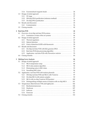


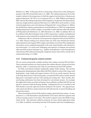
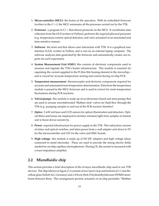
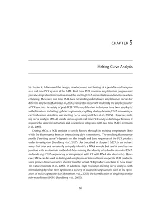
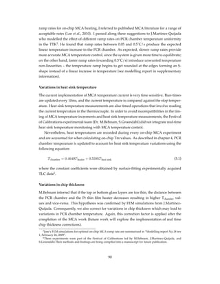
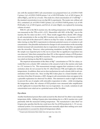
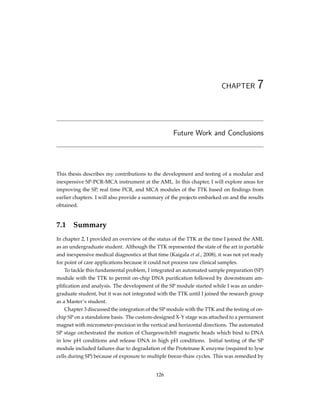
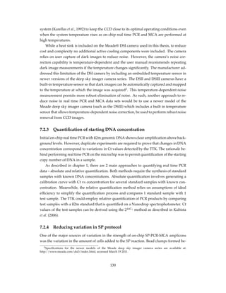
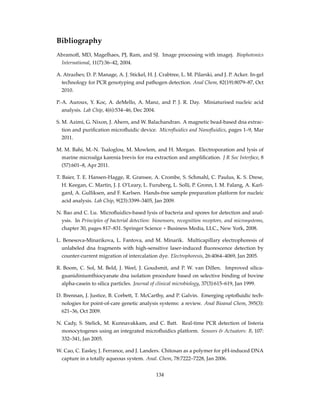
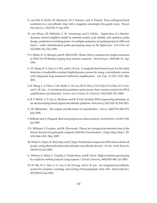
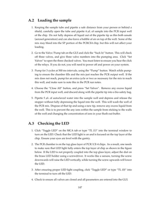
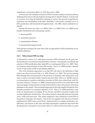
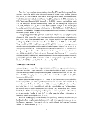
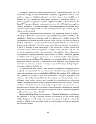
![style” microvalves using mini-pumps integrated with the TTK. The 90µm deep PCR reac-
tion chamber is located on the top glass layer and has a total volume of 600 nL. The design
incorporates a valveless sample preparation channel for DNA purification, and capillary
electrophoresis channels and wells for post-PCR analysis.
2.2.1 Microfabrication protocol
Microchip fabrication is the same as in our past work (Kaigala et al., 2008) but is summarized
here for completeness. Chip designs were completed in L-Edit v3.0 (MEMS Pro 8, MEMS
CAP,CA, USA) and transferred to a photolithography mask using a pattern generator (DWL
200, Heidelberg Instruments, CA, USA). The 4” x 4” glass substrate was first cleaned in hot
Piranha (3:1 of H2SO4:H2O2) cleaning and then coated with 30nm of Cr and 180nm of Au
by sputtering. Next, HPR 504 photoresist (Fujifilm USA Inc., NY, USA) was spun onto the
glass substrate at a spin speed of 500 rpm for 10 s and a spread speed of 4000 rpm for 40 s.
The photoresist-coated substrate was then baked in an oven at 115˚C for 30 min. The next
lithography steps were followed by UV exposure (4 s, 356 nm and with an intensity of 19.2
mW/cm) of the spin- coated substrate through the chrome mask using a mask aligner (ABM
Inc., San Jose, CA, USA) and chemical developing of the photoresist using Microposit 354
developer (Shipley Company Inc. ,Marlborough, MA, USA) for ∼ 25 s. The glass substrate
was etched using hydrofluoric acid [20:14:66 HF(49%): HNO3(70%): H2O], this etch process
has the etch rate of ∼1.1 µm/min. The bottom glass layer (control layer) was etched to a
70 µm depth, and the top glass layer (fluidic layer which includes SP channel, and PCR
chamber) was etched to 90 µm. Finally to glass etching, the masking metals, Cr and Au,
were stripped using Au etch (0.0985M I2+0.6024 M KI) and Cr etch (Arch Chemicals Inc.,
Norwalk, CT, USA).
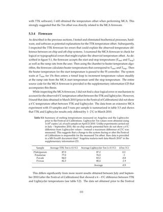
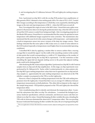
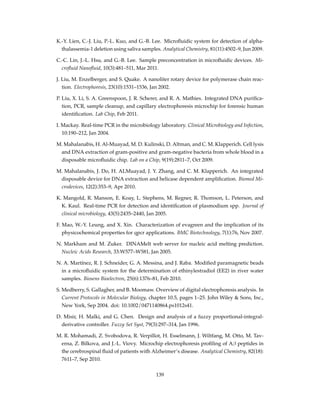
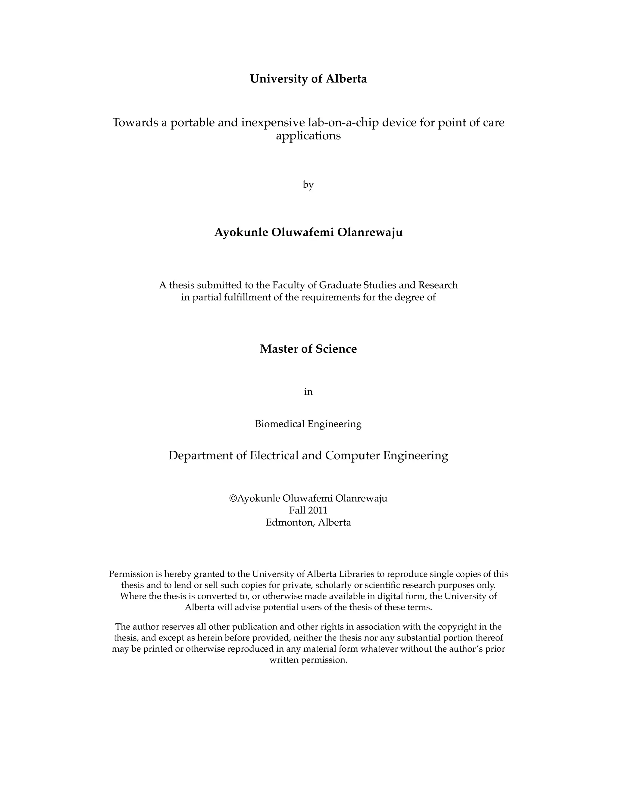
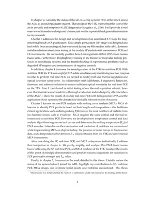
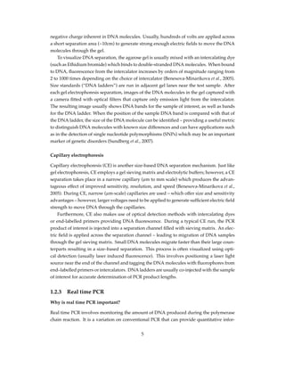
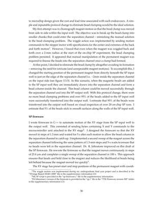
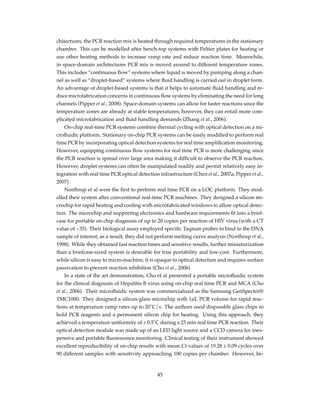
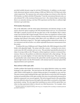
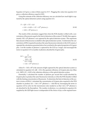
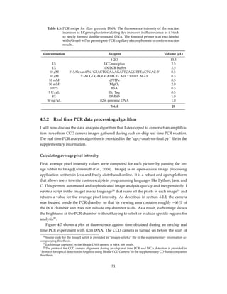
Figure 2.1: Tri-layer microfluidic chip for SP, PCR, and MCA. The chip is made up of 2 Bo-
rofloat glass layers and an intermediate PDMS layer for micro-valve actuation.
Features in red are on the bottom face of top glass layer (“fluidic layer”) where
fluid and magnetic bead movement is performed while features in blue are on
the upper face of the bottom glass layer (“control layer”) where valve actuation
is controlled. The platinum heating/sensing element is etched onto the control
layer of the microchip
To access both fluidic and control channels, portholes were drilled using a Water-jet sys-
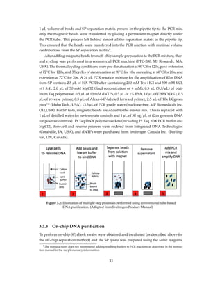
tem (Bengal, Flow International Corp., Kent, WA, USA). To fabricate the micro-heater/sensor,
a Pt film was patterned on the bottom glass layer using “lift-off” technique. After cleaning
14](https://image.slidesharecdn.com/f38dcd23-babd-4fbe-bb5d-16ddc03410a2-150510135757-lva1-app6891/85/Olanrewaju_Ayokunle_Fall-2011-26-320.jpg)
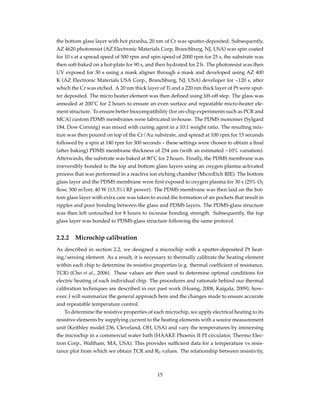


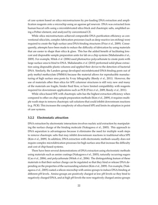
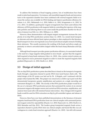
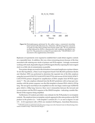
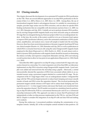
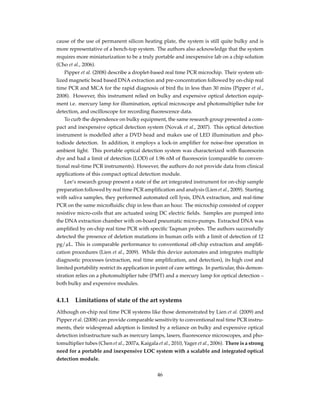
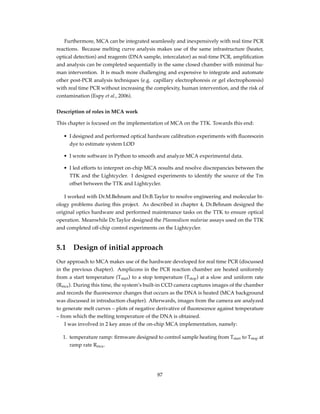
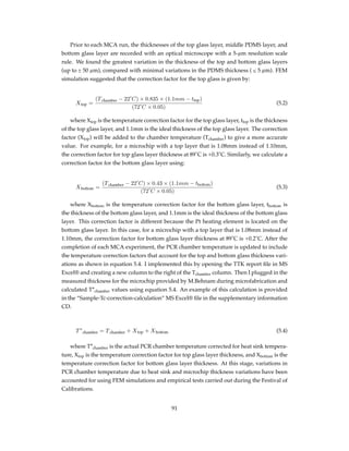
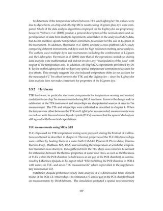
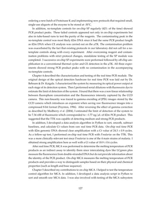
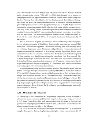
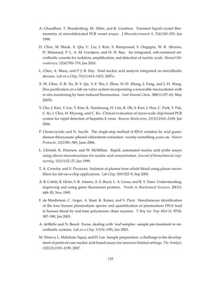
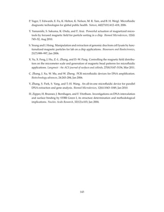
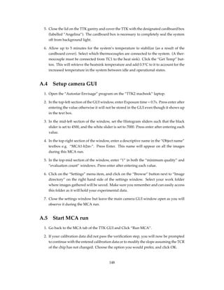
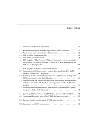
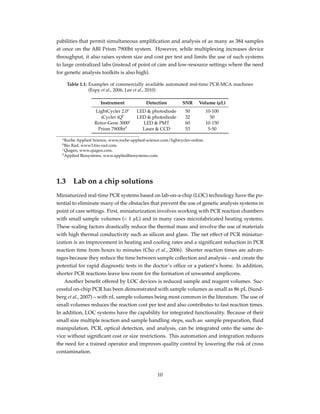
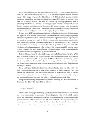
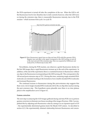
![experiment, and the change in heater resistance corresponding to the current supplied to
the heater.
Step by step derivations of the relationship between the change in heater resistance and
heater temperature are provided in Dr. R. Johnstone’s “Error in Heater Temperature Mea-
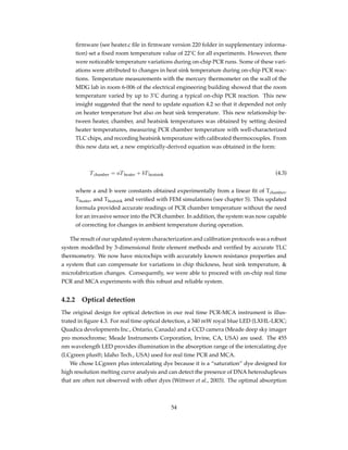
surements using TTKs” report. To summarize, the heater temperature is given by equation
4.1.
Th = Theat sink +
∆Rh
m
(4.1)
where Th is the heater temperature, Theat sink is the heat sink temperature, ∆Rh is the
change in heater temperature, and m is the temperature coefficient of resistance obtained
as the slope of microchip calibration experiments in the water bath described in protocol
11P in the AML microfabrication binder.
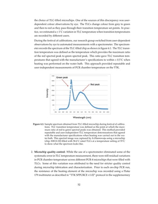
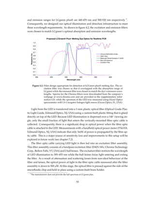
An empirical relationship between heater and chamber temperatures was obtained by
measuring the heater temperature required to obtain colour changes in TLC-filled microchips.
This empirical Tc-Th relationship was used to predict future conversions between heater
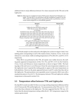
and chamber temperature. S. Poshtiban performed the initial experiments to determine an
empirical relationship between heater and chamber temperatures. Her procedure and re-
sults are summarized in the “Thermal Calibration Report” provided in the supplementary
information CD. I will summarize the key points here.
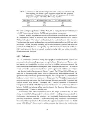
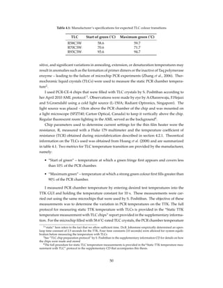
Thermochromic liquid crystals with transition temperatures of 58.6˚C, 70.6˚C, and 93.6˚C
were obtained (R58C3W, R70C3W, R93C3W, Hallcrest, Glenview, IL, USA). Microchips
were filled with the crystals and bonded as described in S. Poshtiban’s “TLC chip prepa-
ration protocol” also provided in the supplementary information. 3 microchips were pre-
pared with the 93.6˚C crystals and the 70.6˚C crystals respectively, while 2 microchips were
filled with the 58.6˚C crystals. The heater temperature was set manually until the TLC crys-
tals were observed to turn green – with observations carried out in a dark room under light
illumination from a cold light source (L-150A; Radiant Optronics, Singapore) placed ~10cm
above the microchip. The room temperature was fixed to 22˚C in the firmware. Using the
data gathered from all 8 microchips, an experimental relationship between the heater and
chamber temperatures was obtained as shown in equation 4.2.
Tc = 2.15Th − 37.95[˚C] (4.2)
where Tc is PCR chamber temperature and Th is heater temperature.
Temperature variations
Prior to on-chip real time PCR experiments, TLC measurements on the TTK were repeated
to measure the variation in PCR chamber temperature. PCR reactions are temperature sen-
49](https://image.slidesharecdn.com/f38dcd23-babd-4fbe-bb5d-16ddc03410a2-150510135757-lva1-app6891/85/Olanrewaju_Ayokunle_Fall-2011-61-320.jpg)
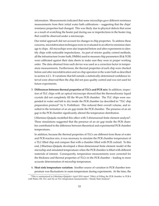
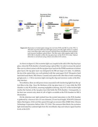

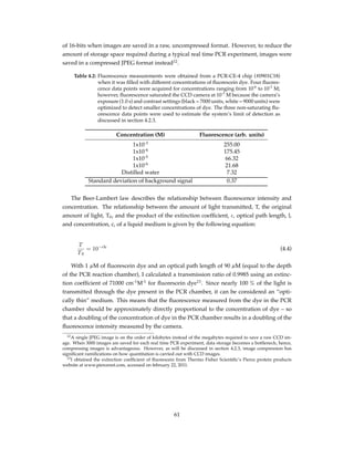
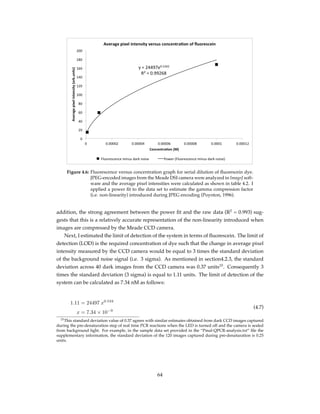
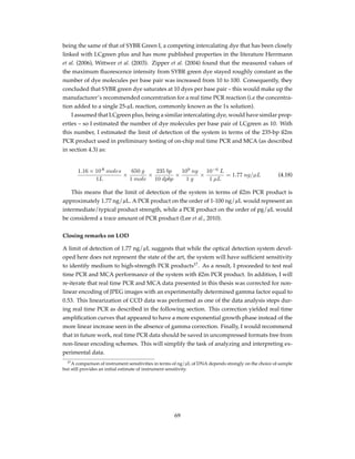
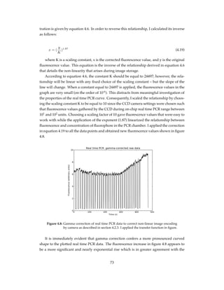
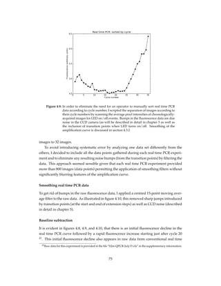
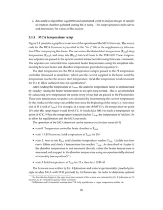
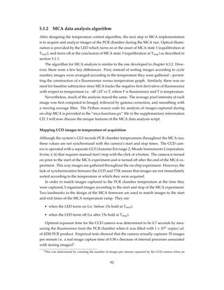
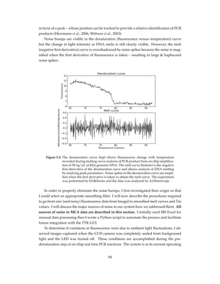
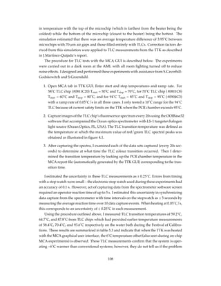
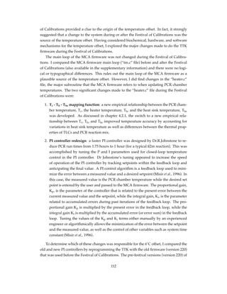
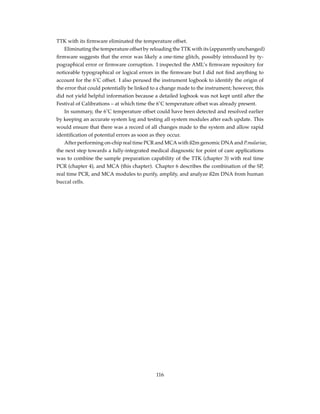
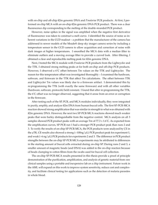
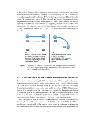
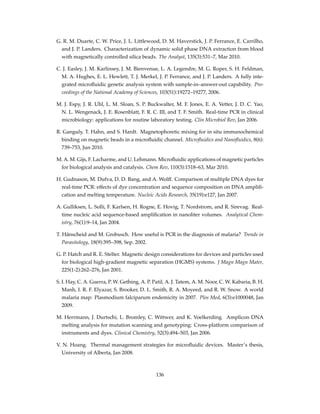
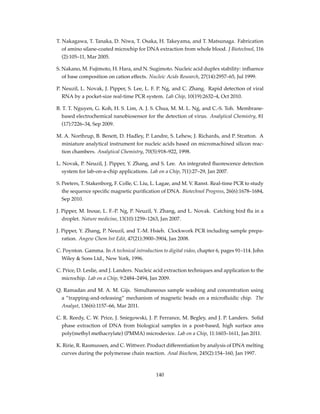
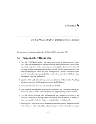
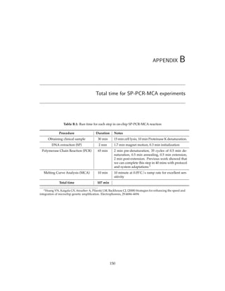
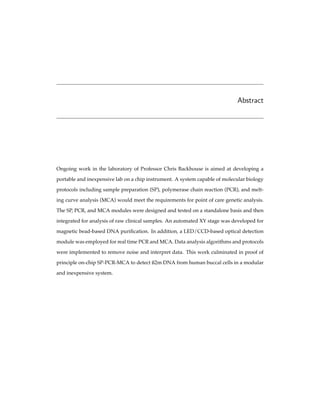
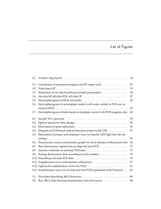
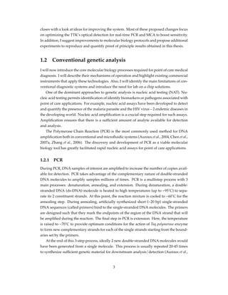
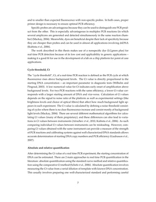
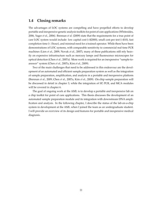
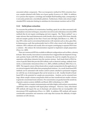
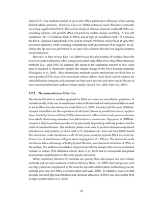
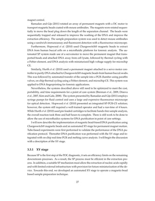
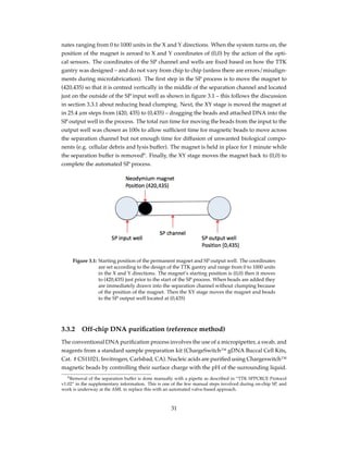
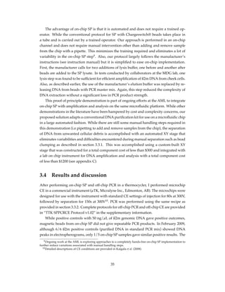
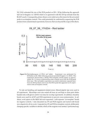
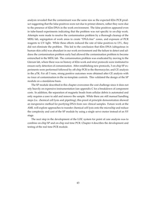
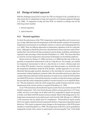
![Figure 4.10: Smoothing real time PCR data. I removed bumps from sorted real time PCR
data by applying with a moving average filter. I identified the source of noise
in the data and described the rationale behind noise removal in chapter 5.1.3.
PCR machines like the Lightcycler and is attributed to temperature-dependent fluorescence
decrease of the intercalator and adsorption of the dye by PCR chamber walls in microchip-
based systems (Cady et al., 2005).
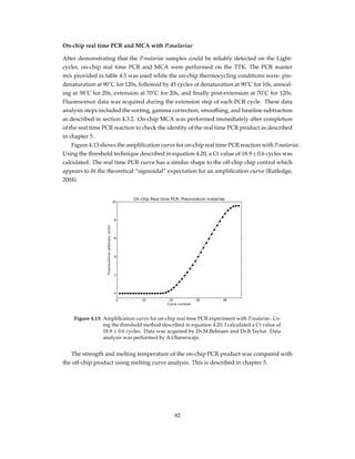
Baseline correction to eliminate this dye-dependent fluorescence decrease is common in
the literature (Neuzil et al., 2010, Rutledge, 2004, Schefe et al., 2006). As such, data gathered
from a conventional machine usually shows zero fluorescence during this initial decline pe-
riod, and then begins to show non-zero increasing fluorescence values once the fluorescence
stops decreasing. This allows the user to ignore the ever-present fluorescence decrease and
focus on important features of the amplification curve such as the cycle threshold.
Real time PCR curves are usually U-shaped, with the left side representing the gently
sloping fluorescence decrease due to dye effects, and the right side representing the rapid
exponential fluorescence increase as double stranded DNA is made. Rutledge (2004) sug-
gest defining the baseline as the minimum point of the real time PCR curve (usually some-
where near the middle of the curve) and setting the fluorescence of all the cycles leading up
to this point to zero. Next, the minimum value is subtracted from all fluorescence values
obtained in cycles after the minimum point.
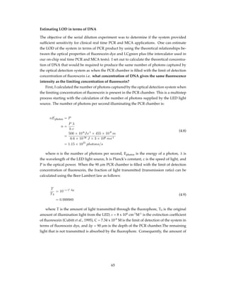
This was implemented in Python as follows:
# ‘ ‘ data ’ ’ i s an array c o n t a i n i n g r e a l time PCR f l u o r e s c e n c e v a l u e s
min_index = data . argmin ( )
min_value = data . min ( )
# equate a l l v a l u e s b e f o r e min_index to 0 s i n c e f l u o r e s c e n c e i s d e c r e a s i n g
for i in range (0 , min_index ) :
data [ i ] = 0
76](https://image.slidesharecdn.com/f38dcd23-babd-4fbe-bb5d-16ddc03410a2-150510135757-lva1-app6891/85/Olanrewaju_Ayokunle_Fall-2011-88-320.jpg)
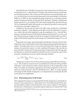
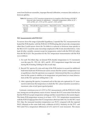
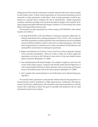
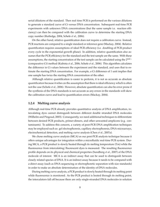
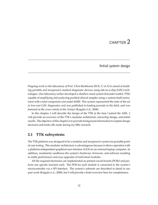
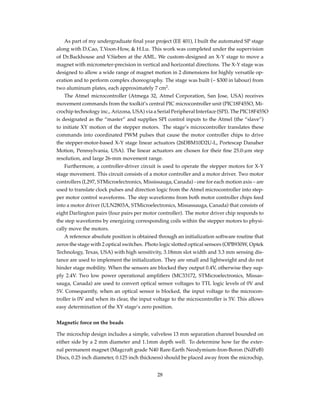
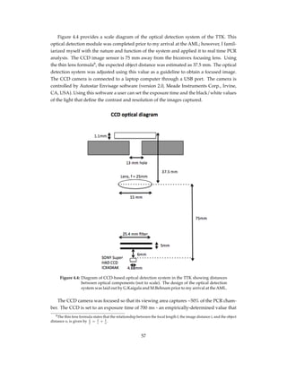
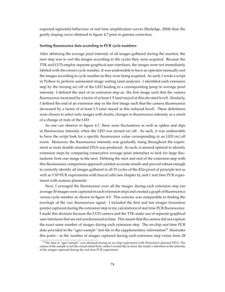
![# s u b t r a c t min_value from a l l v a l u e s a f t e r min_index to remove b a s e l i n e
for i in range ( min_index , size ( data ) ) :
data [ i ] −= min_value
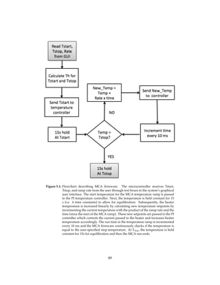
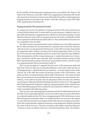
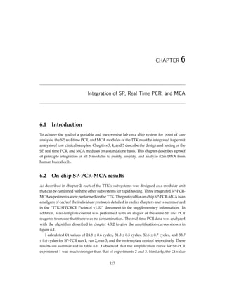
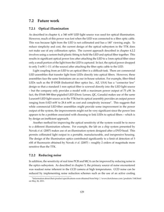
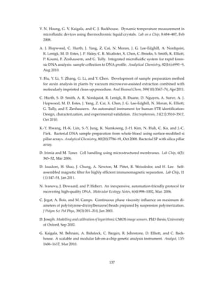
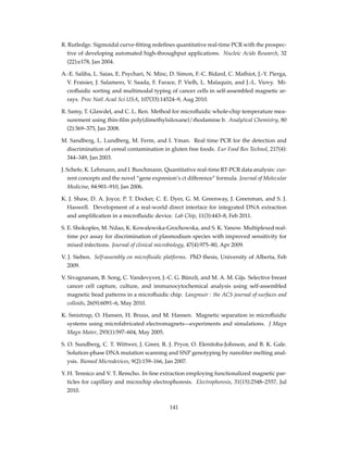
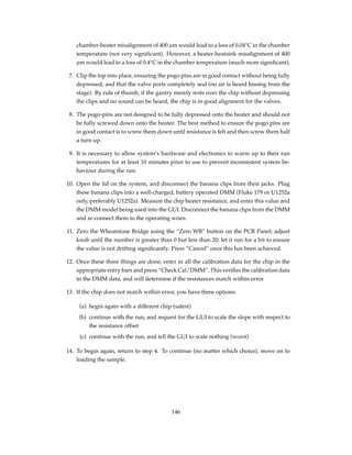
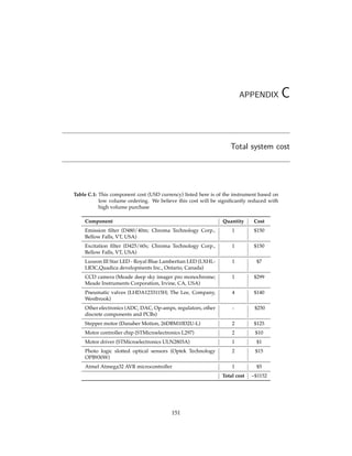
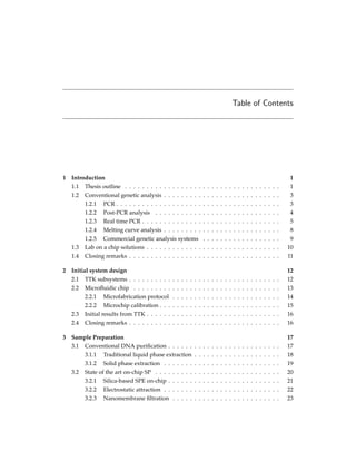
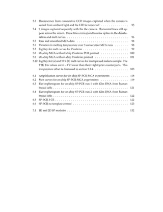
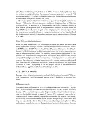
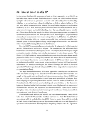
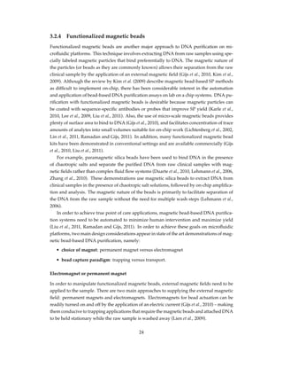
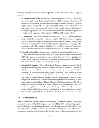
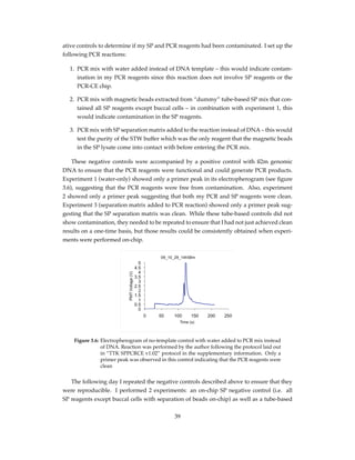
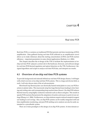
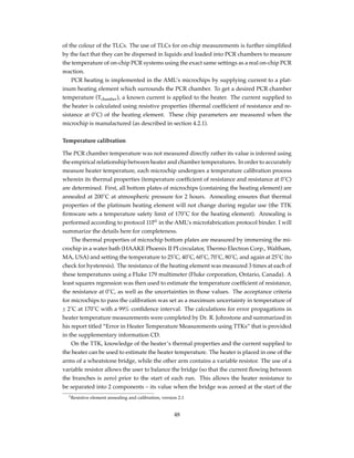
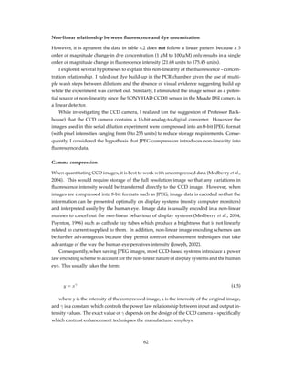
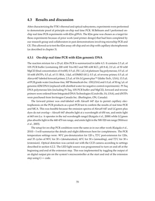
Using this simple baseline subtraction approach, I removed the initial fluorescence de-
cline and plotted the amplification curve with a focus on the fluorescence increase as shown
in figure 4.11. This allowed examination of important features of the real time PCR reaction
such as the calculation of the cycle threshold (Ct value) as described in chapter 1.
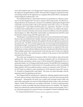
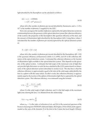
Figure 4.11: The baseline of the amplification curve was removed as described in section
4.3.2, to remove the initial fluorescence decline that is also observed in con-
ventional systems using a simple minimum-subtraction technique described
by Rutledge (2004).
Calculating the Ct value
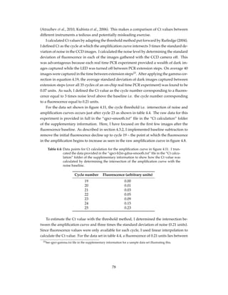
The Ct value is defined as the cycle at which real time PCR fluorescence exceeds background
levels (Mackay, 2004). As described in chapter 1, the Ct value is directly proportional to
the starting DNA concentration – an important parameter in diagnostic tests (Wilhelm and
Pingoud, 2003). A low numerical value for Ct indicates early onset of amplification above
background levels. For two PCR reactions with the same efficiency, a lower Ct value cor-
responds with a larger starting amount of DNA and vice-versa (Gudnason et al., 2007).
One approach to calculating the Ct value involves defining a noise threshold that en-
compasses the fluorescence from cycles where there is no clear fluorescence increase. This
noise threshold usually also includes a measure of fluorescence variation within a cycle
as a result of the signal to noise ratio of the instrument in use (Mackay, 2004). There are
several different mathematical algorithms for calculating Ct values (many of them propri-
etary), and these differences can also lead to variations in Ct values between instruments
77](https://image.slidesharecdn.com/f38dcd23-babd-4fbe-bb5d-16ddc03410a2-150510135757-lva1-app6891/85/Olanrewaju_Ayokunle_Fall-2011-89-320.jpg)