Final_project_watermarked

Electronics and Computer Science
Faculty of Physical Sciences and Engineering
University of Southampton
by Norbert D. Naskov
May 4, 2016
Evaluating Cochlear Implant’s Microphone Acoustic
Performance in an Uncontrolled Environment
Supervisor: Dr. Mark Weal
Second Examiner: Dr. Pawel Sobocinski
A project progress report submitted for the award of
BSc Computer Science
U
niversity
ofSoutham
pton
by
N
orbertN
askov

Abstract
This paper examines the suitability of Frequency Response as an objective mea-
surement for assessing the Cochlear Implant microphone’s current performance,
within an uncontrolled environment. The tests were performed using Advanced
Bionics Nada Cochlear Implant.
A series of tests were developed for assessing the repeatability of the measurement,
as well as the impact of di↵erent factors noise; environment (e.g. Bedroom, Ane-
choic Room, Living room); position of the microphone in relation to the speaker;
ambient noise; di↵erent speaker. Importantly, the measurements acquired with
this method, are not absolute measurements but instead are relative and can only
be used within the context of this application.
Two types of analysis were carried out ﬁrstly, measuring the repeatability of
each test and secondly, comparing the variance that each variable introduces, in
comparison to a base test.
The results show a high repeatability of the tests in all environments, as well
as using di↵erent speakers <1dB variance in each frequency. However, when the
position of the microphone changes and when there is signiﬁcant noise, the variance
between each test, under the same conditions, increases - >2.5dB variance.
Even so, the results show that the Frequency Response measurement can be used in
uncontrolled environments, such as CI users homes, and provide a more objective
overview of the CI microphones performance.
i
U
niversity
ofSoutham
pton
by
N
orbertN
askov

Contents
List of Figures iii
Acknowledgements vi
1 Introduction 1
1.1 Context and motivation . . . . . . . . . . . . . . . . . . . . . . . . 1
1.2 Purpose of this project . . . . . . . . . . . . . . . . . . . . . . . . . 2
2 Background and Current Technologies 3
2.1 Acoustics and the human ear . . . . . . . . . . . . . . . . . . . . . 3
2.2 Digital Signal processing . . . . . . . . . . . . . . . . . . . . . . . . 4
2.3 Hardware description . . . . . . . . . . . . . . . . . . . . . . . . . . 5
2.4 Hearing aid testing standards . . . . . . . . . . . . . . . . . . . . . 7
2.5 Frequency response . . . . . . . . . . . . . . . . . . . . . . . . . . . 7
2.6 TS, TRS, TRRS . . . . . . . . . . . . . . . . . . . . . . . . . . . . 8
3 Implementation and Design 10
3.1 User Interface description . . . . . . . . . . . . . . . . . . . . . . . 10
3.2 Measurement points . . . . . . . . . . . . . . . . . . . . . . . . . . 11
3.3 Syncing . . . . . . . . . . . . . . . . . . . . . . . . . . . . . . . . . 12
3.4 Project management . . . . . . . . . . . . . . . . . . . . . . . . . . 12
3.4.1 Risk assessment . . . . . . . . . . . . . . . . . . . . . . . . . 12
3.4.2 Time management . . . . . . . . . . . . . . . . . . . . . . . 13
4 Evaluation 15
4.1 Method . . . . . . . . . . . . . . . . . . . . . . . . . . . . . . . . . 15
4.2 Dependent variable . . . . . . . . . . . . . . . . . . . . . . . . . . . 16
4.3 Independent variables . . . . . . . . . . . . . . . . . . . . . . . . . . 16
4.3.1 Category 1 Environment variables . . . . . . . . . . . . . . 16
4.3.1.1 Position of the microphone in relation to the mi-
crophone . . . . . . . . . . . . . . . . . . . . . . . 16
4.3.1.2 Distance between speaker and microphone . . . . . 17
4.3.1.3 Noise . . . . . . . . . . . . . . . . . . . . . . . . . 17
4.3.1.4 Surroundings . . . . . . . . . . . . . . . . . . . . . 18
4.3.1.5 Speaker . . . . . . . . . . . . . . . . . . . . . . . . 18
4.3.2 Category 2 Real scenario simulation . . . . . . . . . . . . . 18
ii
U
niversity
ofSoutham
pton
by
N
orbertN
askov

CONTENTS iii
4.3.3 Category 3 Syncing variables . . . . . . . . . . . . . . . . . 19
4.4 Controlled variables . . . . . . . . . . . . . . . . . . . . . . . . . . . 21
4.5 Data collection . . . . . . . . . . . . . . . . . . . . . . . . . . . . . 21
5 Results 22
5.1 Syncing . . . . . . . . . . . . . . . . . . . . . . . . . . . . . . . . . 23
5.2 Null measurement . . . . . . . . . . . . . . . . . . . . . . . . . . . . 23
5.3 Repeatability of the measurement . . . . . . . . . . . . . . . . . . . 23
5.3.1 Category 1 Environment Variables . . . . . . . . . . . . . . 24
5.3.2 Category 2 testing with di↵erent microphones . . . . . . . . 25
5.4 Comparison with base test . . . . . . . . . . . . . . . . . . . . . . . 26
5.4.1 Category 1 Environment variables . . . . . . . . . . . . . . 26
5.4.1.1 Environment . . . . . . . . . . . . . . . . . . . . . 26
5.4.1.2 Position . . . . . . . . . . . . . . . . . . . . . . . . 27
5.4.1.3 Noise . . . . . . . . . . . . . . . . . . . . . . . . . 27
5.4.1.4 Speakers . . . . . . . . . . . . . . . . . . . . . . . . 27
5.4.2 Category 2 testing with di↵erent microphones . . . . . . . . 28
6 Discussion 29
6.1 Limitations . . . . . . . . . . . . . . . . . . . . . . . . . . . . . . . 31
6.1.1 Fundamental acoustic problem . . . . . . . . . . . . . . . . . 31
6.1.2 Relative measurements . . . . . . . . . . . . . . . . . . . . . 32
6.1.3 Syncing . . . . . . . . . . . . . . . . . . . . . . . . . . . . . 33
6.2 Future work . . . . . . . . . . . . . . . . . . . . . . . . . . . . . . . 34
7 Conclusion 35
Bibliography 35
Appendix 1 38
U
niversity
ofSoutham
pton
by
N
orbertN
askov

List of Figures
2.1 Nyquist theorem and aliasing.[5] . . . . . . . . . . . . . . . . . . . . 5
2.2 Frequency and time domains visual explanation.[4] . . . . . . . . . 5
2.3 A full Nada Cochlear Implant with T-Mic 2. . . . . . . . . . . . . 6
2.4 Nada Cochlear Implant with Listening Check. . . . . . . . . . . . . 6
2.5 GN Otometrics Aurical Plus Test chamber and Measurement Mi-
crophone . . . . . . . . . . . . . . . . . . . . . . . . . . . . . . . . 6
2.6 A Frequency Response Graph . . . . . . . . . . . . . . . . . . . . . 7
2.7 TS, TRS, TRRS . . . . . . . . . . . . . . . . . . . . . . . . . . . . 8
2.8 TS, TRS, TRRS CITA . . . . . . . . . . . . . . . . . . . . . . . . . 8
2.9 TRRS male to TRS + TRS female splitter . . . . . . . . . . . . . . 9
3.1 Comparing tests . . . . . . . . . . . . . . . . . . . . . . . . . . . . . 10
3.2 Main Screen . . . . . . . . . . . . . . . . . . . . . . . . . . . . . . . 11
3.3 Risk Assessment . . . . . . . . . . . . . . . . . . . . . . . . . . . . . 13
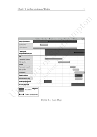
3.4 Gantt Chart . . . . . . . . . . . . . . . . . . . . . . . . . . . . . . . 14
4.1 Final Set up for the experiment . . . . . . . . . . . . . . . . . . . . 16
4.2 Mic on the side of speaker . . . . . . . . . . . . . . . . . . . . . . . 17
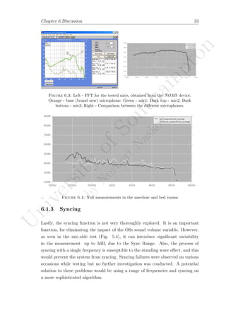
4.3 FFT for the tested mics, obtained from the NOAH device. Orange
- base (brand new) microphone; Green - mic1; Dark top - mic2;
Dark bottom - mic3 . . . . . . . . . . . . . . . . . . . . . . . . . . . 19
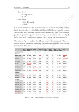
4.4 Conducted tests and relevant variables . . . . . . . . . . . . . . . . 20
4.5 External USB sound card . . . . . . . . . . . . . . . . . . . . . . . 21
5.1 Point variance . . . . . . . . . . . . . . . . . . . . . . . . . . . . . . 22
5.2 Results for the Sync experiment . . . . . . . . . . . . . . . . . . . . 23
5.3 Results for the Repeatability . . . . . . . . . . . . . . . . . . . . . . 24
5.4 The 5 measurements of the mic side test . . . . . . . . . . . . . . . 25
5.5 The 5 measurements of the noise 70dB test . . . . . . . . . . . . . . 25
5.6 Results compared with base tests. Split in octaves . . . . . . . . . . 26
5.7 Base test with mic side and far mic comparison . . . . . . . . . . . 27
5.8 Comparison between the di↵erent microphones. . . . . . . . . . . . 28
6.1 Di↵erence in Octave 5 (4-8 kHz) between Base, Anechoic and Living
room tests . . . . . . . . . . . . . . . . . . . . . . . . . . . . . . . . 30
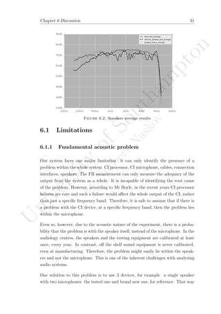
6.2 Speakers average results . . . . . . . . . . . . . . . . . . . . . . . . 31
iv
U
niversity
ofSoutham
pton
by
N
orbertN
askov

LIST OF FIGURES v
6.3 Left - FFT for the tested mics, obtained from the NOAH device.
Orange - base (brand new) microphone; Green - mic1; Dark top -
mic2; Dark bottom - mic3; Right - Comparison between the di↵er-
ent microphones. . . . . . . . . . . . . . . . . . . . . . . . . . . . . 33
6.4 Null measurements in the anechoic and bed rooms . . . . . . . . . . 33
U
niversity
ofSoutham
pton
by
N
orbertN
askov

Acknowledgements
I want to personally thank my supervisor Dr Mark Weal and the principal in-
vestigator of the remote care package Dr Helen Cullington for the immense help
with this project. Without their feedback and guidance, this project would not
have been as successful as it is now.
Furthermore, I want to thank Mr Patrick Boyle and his company Advanced Bionics
LLC, for supplying the required hardware and giving invaluable feedback during
the requirements gathering phase. Without their strong cooperation, this research
would not have been possible.
Lastly, the kind sta↵ of the University of Southampton Auditory Implant Service
Centre for their help and cooperation with the administrative tasks and during
the evaluation phase.
vi
U
niversity
ofSoutham
pton
by
N
orbertN
askov

Chapter 1
Introduction
1.1 Context and motivation
Cochlear implants (CI) are small electronic devices, which completely substitute
the function of a fully damaged ear [9]. In the UK, there are around 12,000 CI
users [8] and these numbers are growing steadily. Currently, only 5% of people
who would beneﬁt are using an implant [2].
Implant services commit to a lifetime post-operative care for CI users, which in-
cludes rehabilitation, device adjustments, hearing tests, etc. However, such care
can only be provided at one of the approximately 20 tertiary centres across the
UK. Typically, patients are required to attend the designated centre once every
year, to carry out the tests. This results in a costly, clinician-centred pathway
that proves ine cient in responding to immediate problems that patients might
be experiencing [1].
One way of dealing with these problems is to implement a patient-centred, remote-
care support package. Such a project is currently being developed by Dr Helen
Cullington and her team [10]. The main purpose of the package is to provide
patients with tools to support remote analysis of their CI and their hearing ex-
perience at the convenience of their home. This paper is a contribution to this
remote-care package.
Initially, two meetings were made with Dr Cullington and Mr Patrick Boyle, a
Hardware Engineer at Advanced Bionics LLC, in which a problem with the Nada
CI device was identiﬁed. Over time the CI’s microphone su↵ers gradual degra-
dation in its performance, especially in the higher frequencies, due to the natural
1
U
niversity
ofSoutham
pton
by
N
orbertN
askov

Chapter 1 Introduction 2
wear of the device and external environmental factors [6]. Since this phenomenon
happens slowly and over time, it is inherently di cult for patients to identify
it. Furthermore, patients sometimes experience problems di↵erentiating between
normal and abnormal behaviour of the device, since they already have a hearing
impairment.
Currently, Nada CI allows for only one way of testing the microphones performance
at home. An unaided user can listen to the current live output, using earphones,
and can do manual, unstructured tests, to make an overall judgment of the hearing
experience (more details in Section 2.3).
1.2 Purpose of this project
The purpose of the project is to investigate, whether a CI user can achieve better
estimation of the microphones performance in uncontrolled environments, such
as their home, with no or relatively cheap additional hardware. Speciﬁcally, to
identify which factors need to be taken into consideration for obtaining robust
measurements of the microphones current performance. What levels of tolerance
are acceptable when comparing performance measurements in uncontrolled envi-
ronments?
The scope of this project is limited to exploring the immediate context around
these two problems. Its focus is on investigating the feasibility of obtaining Fre-
quency Response measurements in uncontrolled environments for objective com-
parison and determining the CI microphones current performance. A real appli-
cation for CI users would need to investigate many more issues related to design,
information visualisation, etc., which fall outside of the scope for this project.
U
niversity
ofSoutham
pton
by
N
orbertN
askov

Chapter 2
Background and Current
Technologies
Assessing the quality of a microphone requires thinking about both the acoustic
nature of the experiment and the digital representation of an analog signal (Digital
Signal Processing).
2.1 Acoustics and the human ear
Acoustics is a complex matter and analysing acoustic performance is typically
done in highly controlled environments, since many parameters a↵ect the outcome
of any measurement [7].
Speciﬁcally, when sound waves reach the ear or measuring instrument the result-
ing change of pressure can be measured. Sound intensity is usually expressed in
decibels of sound pressure level (dB SPL) and is measured in Pascal (Pa). [14] The
human ear can detect pressures from 20 microPa to 20 Pa, resulting in a range of
1:10,000,000. This large range is represented by the logarithmic scale dB SPL.
The Bel scales, are scales of ratio. Each scale must have a reference point at 0
dB, and the measurements are relative to that reference point. The dB SPL scale
represents the ratio of the measured sound pressure using the threshold of human
hearing as reference point 0dB = 20 microPa. Furthermore, a logarithmic scale
resembles more accurately the way the human hearing system interprets sound
loudness.
3
U
niversity
ofSoutham
pton
by
N
orbertN
askov

Chapter 2 Background and Current Technologies 4
A microphone is technically an analog to digital converter (ADC), which converts
the continuous audio signal into discrete samples of voltage. Every microphone
has some form of a membrane that gets excited by sound pressure. The movement
of the membrane is converted into voltage, amplified by an amplifier and finally
converted into a digital number. For conversion between the microphones output
and the absolute Sound Pressure Level, the microphone needs to have an accurate
and current reference point to dB SPL scale. Such reference point can only be
acquired using specially designed environment and equipment.
Firstly, an anechoic chamber is one such environment. All the surfaces are suited
for absorbing the sound energy, resulting in significant reduction of sound re-
flections within the room. Secondly, a measurement microphone, is a specially
manufactured and tested microphone, whose frequency response is calibrated and
accurately cross-referenced to the dB SPL scale. Using such measurement mi-
crophone during a test (alongside the tested microphone), allows for obtaining
absolute measurements of the tested microphone, by comparing its relative out-
put to the measurement microphones absolute output. [13]
However, such calibrated equipment is expensive and impractical for home users
to obtain or use. Therefore, the measurements that we obtain are not absolute
and cannot be interpreted as dB SPL, because there is no reference point to an
absolute value in dB SPL. Instead, they are relative measurements and are only
meaningful within the context of our application.
2.2 Digital Signal processing
DSP is a field of computer science that deals with the conversion of analog signals
to digital signals and their storage and processing. Audio Processing is a subfield
of DSP.
The number of samples per second that the microphone takes is called the sample
rate. According to the Nyquist Theorem, we need to sample the analog signal at
a rate at least twice the highest frequency of the signal we are interested in. [15]
The idea behind the sampling theorem is that we need to have at least 2 samples
within a cycle of a component to be able to detect that component. If there are
less than 2 samples per cycle, than the output signal will introduce lower frequency
components, which were not present in the original signal aliasing. (Fig. 2.1)
U
niversity
ofSoutham
pton
by
N
orbertN
askov

Figure 2.1: Nyquist theorem and
aliasing.[5] Figure 2.2: Frequency and time
domains visual explanation.[4]
Human hearing is limited to the range of 20Hz to 20kHz [14]. Therefore, the
standard sample rate of 44.1 kHz has emerged, capable of capturing all audible
signals of the human ear. This means that the microphone creates 44,100 integer
(standard is 16 bit) samples per second, representing the amplitude of the signal
at that particular moment of time. Combining the samples together in an array,
represents the audio signal in the time domain.
However, according to the Fourier Theorem, any periodic signal can be decom-
posed into a series of sines and cosines, with di↵erent frequencies, amplitudes and
phases. This decomposition of the signal renders the same signal in another do-
main the frequency domain. The Fourier Transform is a transform, which converts
a signal from the time domain to the frequency domain. [16] (Fig. 2.2) Both rep-
resentations are equivalent to each other and encode the same information about
the signal. However, the frequency domain allows for di↵erent types of analysis
and manipulation of the signal. The Fourier Transform for discrete signals is called
Discrete Fourier Transform and the implementation of the DFT, called the Fast
Fourier Transform FFT, is widely used within the DSP ﬁeld. [16]
In the context of our project, we create a frequency response graph, by analysing
the magnitude of the di↵erent frequency components of the input signal.
2.3 Hardware description
Fig.2.3 shows an overview of the Nada Cochlear Implant. This device was provided
by Advanced Bionics LLC to conduct the tests. The tested CI device consisted of
the following components: Nada CI Q70 (CI-5245) processor; PowerCel battery
110; T-Mic 2 Large; CI-5823 Nada CI Listening Check.
U
niversity
ofSoutham
pton
by
N
orbertN
askov

The Nada CI, comes with an external module Listening Check, (Fig. 2.4) which
allows the audio to be output via 3.5mm TRS interface. (3.5mm Jack with stereo
output). At home, the CI device is tested manually from a person without a
hearing impairment, by using earphones and subjectively assessing the quality
of the sound input. Users test the device by talking” to the microphone and
making di↵erent sounds to get a feel of the hearing experience. This method is
clearly subjective and error-prone but provides a quick and easy way for testing the
device. Unfortunately, employing such a method proves hard in unambiguously
identifying problems with the performance and is only suitable for outlining a
general overview of the sound quality.
Figure 2.3: A full Nada Cochlear Implant with T-Mic 2.
Figure 2.4: Nada Cochlear Im-
plant with Listening Check.
Figure 2.5: GN Otometrics Au-
rical Plus Test chamber and Mea-
surement Microphone
U
niversity
ofSoutham
pton
by
N
orbertN
askov

In contrast, at the University of Southampton’s Auditory Implant Centre, CI’s
microphone performance is tested using special equipment like GN Otometrics Au-
rical Plus (NOAH ) (Fig. 2.5). The NOAH device has a small isolation chamber,
where the hearing aid is mounted. Also, a measurement microphone (explained
above) is provided and is set up next to the CI. Finally, the CI is connected to a
computer via 2cc coupler, using a 3.5mm stereo jack. The NOAH device includes
a software package and provides various di↵erent tests for assessing the charac-
teristics of the CI Reference Test Gain, Frequency Response Curve, Frequency
Range, Harmonic Distortions and others.
2.4 Hearing aid testing standards
The manual of the NOAH device states that the tests are implemented in accor-
dance to the standard ANSI S3.22-1996. This is not latest version of the standard,
however, since it was revised again in 2003. The standard is created for quality
control purposes. It outlines the di↵erent conditions, which need to be met in
order to perform tests on hearing aids. For the Frequency Response test there are
several requirements in the latest standard and we have implemented the follow-
ing: volume (gain) of the CI is set to Reference Test Setting (RTS); the Automatic
Gain Control (AGC) is turned o↵; the recommended tolerance level of 4dB under
2kHz and 6dB above 2kHz is used in calculating erroneous measurements.
2.5 Frequency response
Figure 2.6: A Frequency Re-
sponse Graph
For the purpose of this project, we fo-
cused on reproducing only one of these
tests the frequency response test (FR).
FR is a measurement of the magnitude
of the input as a function of the fre-
quency. In other words, when we play
a signal at a speciﬁc frequency, what is
the magnitude of the microphones in-
put for that frequency. The result is
plotted on a graph like in Fig. 2.6. The
U
niversity
ofSoutham
pton
by
N
orbertN
askov

Y axis of the graph represents the mag-
nitude (in dB) and the X axis is the frequency (in Hz). Both axes are logarithmic
axes, resembling the human hearing experience.
Assessing the frequency response (FR) of the microphone can give an adequate
overview of its performance. All acoustic tests are performed with pure tone
signals. Although these do not represent the signal that a typical user would be
hearing, pure tone signals are used since analysis on them produces more consistent
results across di↵erent conﬁgurations.
The criteria for determining the quality of the tested CI device is by comparing the
current measurement to a base measurement. Base measurements are obtained
from a brand new CI device (of the same model) either the same device, at the
day of acquiring, or a new device, currently available at the audiology centre.
2.6 TS, TRS, TRRS
It was proposed that a mobile platform, such as an iPhone or iPad, would be a
suitable system to design the project for. However, it turns out that iOS devices
have hardware incompatibility with the Nada CI.
The CI provides an external module called the Listening check (as described
above). Speciﬁcally, this module allows for the output of the CI device to be
accessed via 3.5mm port.
Figure 2.7: TS, TRS, TRRS
Figure 2.8: TS, TRS, TRRS CITA
There are 3 standard
types of 3.5mm con-
nectors TS, TRS,
TRRS (Fig. 2.7), de-
pending on the num-
ber of channels in-
cluded. TS and TRS
do not vary between
manufacturers they
follow the same organ-
isation Audio (Left,
Right) and Ground.
However, when it comes to adding the 4th signal the microphone, there are
U
niversity
ofSoutham
pton
by
N
orbertN
askov

multiple standards OMTP (Open Mobile Terminal Platform), CTIA (Cellular
Telephone Industries Association) and other standards. (Fig. 2.8)
Figure 2.9: TRRS male
to TRS + TRS female
splitter
The incompatibility between the CI and the
iOS devices arise, since Apple have currently
employed the TRRS CITA standard on their
devices both laptops and mobile devices. The
3.5mm socket of any modern Apple device has
a single (mono) input channel at the Sleeve
and two output channels at the Tip and Ring1.
However, the CI outputs a TRS configuration
with left and right (stereo) outputs on the Tip
and Ring1, e↵ectively trying to input its signal
to the output ports of the Apple device. Due
to this incompatibility, using the two devices
directly is impossible. The only available solution to this problem is to use a
TRRS splitter (Fig. 2.9) . The splitter splits the single TRRS port into two TRS
ports one for headphones and one for a microphone.
Using the best splitter on the market (according to Amazon user reviews) this
configuration for bridging the CI device and the iPhone was tested. However, the
input from the CI was received with considerable breaks of the signal e.g. 0.2s
of data with 0.8s of null data, and after a few seconds, the data completely stops.
The tests were conducted on an iPhone 5, iPad 2 and iPad 3. All 3 iOS devices
experienced the same problems. On the other hand, using the same set up (CI
and splitter) with a MacBook Pro, which also has the same TRRS jack, does not
exhibit these data loss issues.
These findings suggest there is a limitation within the iOS system itself. Hence,
further iOS compatibility was not investigated. Instead, the test was conducted
using OS X and MacBook Pro.
U
niversity
ofSoutham
pton
by
N
orbertN
askov

Chapter 3
Implementation and Design
To analyse the Frequency Response, a Python app was built. The Python lan-
guage was chosen, since one of the requirements for the project is portability.
Python is available on all major OS-s. Furthermore, the availability of the pack-
age Scipy/Numpy makes Python is very well suited language for building scien-
tiﬁc prototypes. Almost every function for DSP, data analysis and manipulation
is available in these packages. For visualisation purposes, the package Matplotlib
was used.
3.1 User Interface description
Figure 3.1: Comparing tests
The application focuses only on facili-
tating the execution of an experiment
and appropriately visualising the re-
sults. It is not targeted at end users,
since this is outside of the scope of this
project. It consists of two windows
one is the main frame (Fig. 3.2) of the
application, where the researcher can
run a new test, load a test and com-
pare two di↵erent tests. The second
window shows the speciﬁc comparison
between the tests, highlighting the er-
rors between the two tests. (Fig. 3.1)
10
U
niversity
ofSoutham
pton
by
N
orbertN
askov

Chapter 3 Implementation and Design 11
Figure 3.2: Main Screen
An important detail of the implementation is the Sync function (see Section 3.3).
The user can choose to do a test with or without the sync function.
Syncing eliminates one of the variables of the test the OSs sound output. The
function automatically adjusts the sound output to reach a predeﬁned level for
the Sync Frequency.
3.2 Measurement points
As mentioned above, the test consists of measurements of the magnitude for each
frequency. 5 octaves of frequencies were used and within each octave 16 fre-
quency points were measured. A Perfect Octave by deﬁnition (ANSI/ASA S1.1-
2013 Acoustical Terminology) ranges from a start frequency to an end frequency,
which is double the start. We have not used perfect octaves, instead the rounded
octaves were used. (See Appendix 1) The scale was created by taking the lowest
frequency, technically audible by the CI 200Hz, and laying out the 5 octaves on
top with the appropriate frequencies. The technical frequency cut-o↵ of the CI
is at 8kHz but for the sake of completeness, the test frequencies range to 10kHz
with 6 of them above 8kHz. However, these are not taken into account during the
evaluation. There are 74 frequencies in total, between 200Hz and 8kHz.
To make a test, the application simultaneously plays a sound through the speakers
and analyses the input from the CI microphone. The application plays the Test
Frequencies in order and expects to receive them in the input. The magnitude
for each frequency is computed using the FFT of 6 separate bu↵ers, 4096 samples
U
niversity
ofSoutham
pton
by
N
orbertN
askov

each. The final magnitude value for the frequency is taken as the average of the
first two bu↵ers, which have it as the one with the highest amplitude. However,
if there are not two such bu↵ers, then the average amplitude for that frequency
of all 6 bu↵ers is taken. This method minimises the e↵ects of the environment
on the measurement, since the actual measurement is taken as the average over
a significantly long period (0.3s 1s) of pure tone signal. The whole test takes
around 1 minute to complete.
3.3 Syncing
The first step is Syncing. During this step, the app plays a pure tone sound at
only one frequency the Sync Frequency. It adjusts the output volume of the OS
up or down until the magnitude of the Sync Frequency is at the specified level
Sync Level. The Sync Level is a predefined constant at 70dB. There is also a
Sync Range 3dB. These constants were estimated during tests with the device.
A Synchronised State is attained when the following conditions have been met 10
consecutive time:
• the Sync Frequency is the Frequency with the highest magnitude
• the magnitude is Sync Level magnitude Sync Level + Sync Range
The Sync Function does not break portability, even though it alters the OS Volume
Output Setting directly. In Mac OS this is done with a terminal command, however
on a Windows machine, there also exists an external utility to control the output
via command line Nircmd.
Optionally, this step can be skipped and the researched can manually control the
volume of the OS. Even though this is not recommended, it is useful in situations,
where Synced State cannot be attained.
3.4 Project management
This section outlines the techniques and tools used for managing the project.
3.4.1 Risk assessment
U
niversity
ofSoutham
pton
by
N
orbertN
askov

Figure 3.3: Risk Assessment
First of all, a risk
assessment procedure
was carried out to
identify potential risks
with the project and
solutions to mitigate
them. An outline is
given in Fig. 3.3.
The chart describes
the various related risks
and the relevant ac-
tions to diminish them
with a simple scoring
system of 1-5. Unfor-
tunately, not enough
importance was given
on the compatibility
between the CI implant and the iOS device, hence a portion of the time was spent
developing an application for iOS. However, in retrospect, the double implementa-
tion of the algorithms helped me to really deepen and solidify my understanding
of the problem and context around it.
3.4.2 Time management
For time keeping and planning the Gantt Chart proved very helpful in assessing
the progress of the project.(Fig. 3.4) An obvious miscalculation can be observed
with the literature review section. The nature of this project was exploratory and
accessing books and information in relation to DSP and acoustics was necessary
throughout the whole project. Also, it can be observed that the second implemen-
tation took considerably less time for completion, conﬁrming the higher degree of
problem comprehension.
U
niversity
ofSoutham
pton
by
N
orbertN
askov

Figure 3.4: Gantt Chart
U
niversity
ofSoutham
pton
by
N
orbertN
askov

Chapter 4
Evaluation
4.1 Method
The project aims to answer the questions:
• What are the expected levels of tolerance for the accuracy of the measure-
ment?
• What factors do the users need to consider when performing the tests?
Firstly, for estimating the tolerance for accuracy, 5 consecutive measurements of
every test were conducted. The 5 measurements are then compared internally, with
each other, and conclusions are drawn from the results. For comparing di↵erent
tests, ﬁrst the means of the 5 measurements for both tests are taken, and then the
comparison is based on those mean vectors.
The literature shows that the most important factors to consider are:
• the interference of the sound waves with the environment and the objects in
proximity [11] [13]
• the background noise [11] [13]
• the performance of the speaker itself [11]
The next sections discuss the speciﬁc variables, which were examined within this
experiment.
15
U
niversity
ofSoutham
pton
by
N
orbertN
askov

Chapter 4 Evaluation 16
4.2 Dependent variable
The dependent variable is the collection of all measured points (see Section 3.2),
representing the amplitudes of the di↵erent frequencies, also known as the Fre-
quency Response Curve. However, it is important to note that these measured
points are relative and not absolute measurements, since there is no calibrated ab-
solute reference point. These measurements can only be used within the context
of this system.
4.3 Independent variables
Figure 4.1: Final Set up
for the experiment
To investigate the robustness of the measure-
ment, a number of tests were constructed, each
focusing on a di↵erent variable. A photo of the
final set up is shown in Fig. 4.1. The evalua-
tions are split in 3 categories:
4.3.1 Category 1 Environment
variables
This category of tests focuses on exploring the
variation, which the di↵erent environment fac-
tors introduce. The sound waves could easily be altered by the surrounding objects
and the room where the test takes place. Therefore, the importance of the follow-
ing factors was examined:
4.3.1.1 Position of the microphone in relation to the microphone
• On a microphone stand, directly above the speaker (Default)
• On the desk, at the side of the speaker (Fig. 4.2)
The position of the microphone in relation to the speaker is of great significance,
since the sound waves are a↵ected by reflections of the flat surface, as well as by
any objects in proximity. Furthermore, the speaker that we used Minirig, is faced
upwards, towards the ceiling and not sideways, along the desk surface.
U
niversity
ofSoutham
pton
by
N
orbertN
askov

Figure 4.2: Mic on the
side of speaker
Constraints:
The ﬁrst constraint for this variable is that
there are no obstacles between the CI device
and the speaker.
The second constraint is related to the micro-
phone stand. It must be a cylindrical tall ob-
ject, with a relatively small diameter, in order
to prevent interference with the sound waves.
The last constraint is related to the speaker
the speaker must be aimed at the microphone.
4.3.1.2 Distance between speaker and microphone
• 10cm (Default)
• 1m
The distance between the speaker and microphone has an obvious e↵ect on the
measurement. The further the microphone from the speaker, the lower the Signal
to Noise ratio, e↵ectively losing the sound within the background noise.
4.3.1.3 Noise
• Room noise (Default) 52 dB
• Loud noise created with speakers 70dB
• Reduced noise in the anechoic room (anechoic test) 45dB
Clearly the ambient noise of the environment can impact the measurement. There-
fore, di↵erent levels of noise were tested. The noise level in all environments was
measured with a calibrated noise meter, lent from the Audiology Centre. The
loud noise test was measured in the room with UE BOOM speaker, facing the
microphone and the Minirig, playing a Forest and Nature Sounds track [3] , at
level 70dB.
U
niversity
ofSoutham
pton
by
N
orbertN
askov

4.3.1.4 Surroundings
• Room1 (Bedroom) (Default)
• Room2 (Living room)
• Outdoors
• Anechoic room in the audiology centre
The default environment is a typical bedroom, which has a desk, a bed, various
objects on the bed and within the room. The di↵erence between a bedroom and
a living room is relatively small, since both are filled with uncontrolled number
of objects and obstacles for the sound waves. The anechoic chamber in the ISVR
unit was also used for a comparison.
4.3.1.5 Speaker
• Minirig (Default)
• Logitech UE BOOM 2 speaker
• Internal Mac Book Speakers
The speakers play an important role in the whole process. Inevitably, an error with
the speaker itself, will be detected by the microphone. Therefore, a high quality
speaker is recommended. For this experiment the default speaker is Minirig, whose
frequency response is given by the manufacturer as - 75 - 20,000Hz 3dB. This
means that within the range, every tone is within 3dB of any other tone, resulting
in relatively flat frequency response curve, suitable for our purposes.
There are 8 tests in total in Category 1, one for each di↵erent value of the variables.
For each test, only 1 variable was changed and this setup allows for analysis of the
impact from that specific variable only.
4.3.2 Category 2 Real scenario simulation
For a real world test, 3 other T-Mic-s were used. They are known to have some
problems and are collected from the Audiology Centre as dysfunctional. The
brand new T-mics frequency response was compared with the other microphones
responses (Fig. 4.3). Mic1 and Mic2 exhibit similar performance to each other
and to the base microphone, as tested by the Noah equipment . In contrast Mic3
shows clearly noticeable failure, easily distinguishable by a manual check with
headphones almost no sounds are audible.
U
niversity
ofSoutham
pton
by
N
orbertN
askov

This category is used for evaluation of the behaviour of the application with micro-
phones, which are not brand new. Essentially creating a simulation of a realistic
scenario.
Figure 4.3: FFT for the tested mics, obtained from the NOAH device. Orange
- base (brand new) microphone; Green - mic1; Dark top - mic2; Dark bottom -
mic3
4.3.3 Category 3 Syncing variables
The Syncing function was introduced to eliminate one of the variables the variable
volume setting of the OS. A standard for acoustic measurement is to take the base
measurement at 1kHz. Therefore, the same frequency was chosen for the Sync
function. However, the e↵ects of di↵erent Syncing conﬁgurations were investigated
in search for better understanding of the syncing e↵ect on the test. The following
variables were investigated:
• Sync Frequency
– 1000 Hz (Default)
– 1600 Hz
– 2500 Hz
U
niversity
ofSoutham
pton
by
N
orbertN
askov

• Sync Level
– 70 dB (Default)
– 60 dB
• Sync Range
– +3 dB (Default)
– +1.5 dB
It is important to note, that there was only one successful test at 60 dB Sync
Level, since the other two 60+3dB at 1600Hz and 2500Hz, were not able to attain
Synchronised State, since the required output was slightly lower than the lowest
possible output of the speaker. Every reading taken from the speaker was slightly
higher than 63dB even when the speaker was set on the lowest output option.
The table in Fig. 4.4 outlines the di↵erent tests in the experiment. There is a
default value for each of the 9 variables, the combination of which forms the base
measurement base test.
Figure 4.4: Conducted tests and relevant variables
U
niversity
ofSoutham
pton
by
N
orbertN
askov

4.4 Controlled variables
Figure 4.5: External USB sound
card
Firstly, the T-mic is an omnidirectional
microphone and therefore the rotation,
with respect to the speaker, was kept
constant.
Secondly, the connection interfaces be-
tween the computer and the device was
also kept the same and external USB
sound card, built with the HS-100 B
chip. (Fig.4.5) This is a better so-
lution, which on theory provides less
noise then using the splitter. The price of both devices is under 10.
Lastly, the tests were carried out on a single machine - MacBook Pro (13-inch,
Early 2015), running OSX El Capitan 10.11.4 with Python 3.4.3.
4.5 Data collection
For the data collection a new module of the app was build. It automated the data
collection by running the test 5 consecutive times and saving the data into ﬁles.
For each test, the independent variable was conﬁgured and then the automation
module was run.
U
niversity
ofSoutham
pton
by
N
orbertN
askov

Chapter 5
Results
The analysis of the data was done by using the Python library Numpy. It is an
e↵ective tool for dealing with and analysing scientific data. The choice was made
primarily due to the ease of integration with test data. For more sophisticated
analysis and visualisation, tools like IBM SPSS or the R Language would be more
suitable. In the context of this project, however, Pythons Numpy was su cient.
For visualisation, Microsoft Excel was used.
Figure 5.1: Point variance
A definition for Point Vari-
ance (PV) is given as the
di↵erence between the maxi-
mum and minimum measure-
ment for a specific frequency,
from a subset of tests. PV is
calculated for each frequency
under 8kHz and is measured in
dB. (Fig. 5.1) Average Point
Variation is denoted as avgPV.
Two di↵erent analysis were
completed. One of them fo-
cuses on the repeatability of
each test and the other one calculates the variation of the di↵erent tests in com-
parison to the base test.
22
U
niversity
ofSoutham
pton
by
N
orbertN
askov

Chapter 5 Results 23
5.1 Syncing
Exploration of the Sync Function was conducted at the beginning, to gain under-
standing of the e↵ects and choose the most suitable parameters. It was tested
by changing the di↵erent sync parameters Sync Frequency, Sync Level and Sync
Range. The test name denotes all three parameters e.g. sync 1000 60+3 is a test
performed at 1000 Hz Sync Frequency, 60 dB Sync Level and 3dB Sync Range.
The conﬁguration, which exhibits the lowest variation with the lowest number of
outliers was chosen. (Fig. 5.2)
Figure 5.2: Results for the Sync experiment
5.2 Null measurement
Two null measurements were made one in the Bedroom (default) and another
one in the anechoic room. A null measurement is a measurement, which records
the ambient noise of the environment and there is no output from the application.
The microphone is on the stand. These measurements represent the noise of the
system and the environment.
5.3 Repeatability of the measurement
Firstly, analysis on the repeatability of the tests was carried out. In this scenario,
PV is calculated based on the 5 runs of the same test. (Fig. 5.1) Speciﬁcally,
robustness of the tests was estimated by calculating the avgPV, across all fre-
quencies. This analysis provides an overview of how much di↵erence between
U
niversity
ofSoutham
pton
by
N
orbertN
askov

separate measurements can be expected when repeating a test under the same
conditions. Furthermore, the number of points, for which the PV is higher than a
tolerance, are also plotted. This is useful for analysing the extremes within a test.
All tests are outlined in Fig. 5.3.
Figure 5.3: Results for the Repeatability
5.3.1 Category 1 Environment Variables
All tests proved very high repeatability factor under 2.5dB of Point Variance
among the repeated measurements. The least repeatability was observed from the
tests for microphone/speaker position (mic side with avgPV of 2.5dB) and high
noise (noise 70dB with avgPV of 2.3dB). Further investigation in the mic side
test (Fig. 5.4) reveals that one of the measurements mic side 4, was measured
slightly higher than the other 4 tests. This suggests that the error is due to the
syncing function it was synced at a slightly higher output volume. Therefore, for
this speciﬁc test if we take the average of the other 4 tests, we get an avgPV for
mic side of 1.0dB.
In comparison, within the noise test we do not see the same behaviour. Instead
we can observe a more uniform distribution of variance between the di↵erent mea-
surements. (Fig. 5.5)
Lastly, it can be observed that among all tests there is only one outlier, the PV of
which is higher than 6 dB around 7kHz in noise 70dB 2 test. (Fig. 5.5) All other
U
niversity
ofSoutham
pton
by
N
orbertN
askov

Figure 5.4: The 5 measurements of the mic side test
Figure 5.5: The 5 measurements of the noise 70dB test
tests, show steadily declining trend of number of points with PV higher than a
tolerance, when increasing the tolerance.
5.3.2 Category 2 testing with di↵erent microphones
The secondhand microphones were tested with the default values for all environ-
ment variables. All exhibit a high measurement repeatability, even the clearly
dysfunctional microphone Mic3. This is expected but important fact, proving the
accuracy of the system.
U
niversity
ofSoutham
pton
by
N
orbertN
askov

5.4 Comparison with base test
The second analysis estimates the impact that each independent variable has on
the measurement, in comparison to the base test. Here, an average measurement
for each test is taken, as the mean vector from the 5 individual runs. The com-
parison is then calculated using those averaged vectors between the base test and
the other test, in question. Within the context of this analysis, a test refers to the
averaged vector. Also, PV indicates the di↵erence in magnitude measurements for
a given frequency, only between the base and the other test, in question.
Two measurements are given the avgPV and number of errors. Errors in this
context, are taken from the ANSI standard, as PV >4dB at and under 2kHz and
PV >6dB above 2kHz. The measurements are calculated separately for each oc-
tave, to give more precise understanding of the di↵erences at the di↵erent sections
across the whole spectrum.
Figure 5.6: Results compared with base tests. Split in octaves
5.4.1 Category 1 Environment variables
By changing only one variable and comparing it with the base test, we can ap-
proximate the impact of that speciﬁc variable.
5.4.1.1 Environment
According to the results, the environment has a minimal e↵ect on our system. The
Anechoic room, Living room and Outdoors exhibit only 0.6dB, 0.7dB and 1.2dB
of average Point Variation. Obviously, the noisier the environment (Outdoors)
the higher the PV for test. Interestingly, the base test in a Bedroom only di↵ers
U
niversity
ofSoutham
pton
by
N
orbertN
askov

minimally 0.6dB compared to a test made in anechoic room. However, no errors
were observed from changing the environment.
5.4.1.2 Position
The position (mic side) and the distance (far mic) of the microphone, in relation to
the speaker, are the most important variables for our system (avgPV of 4.5dB and
5.3dB and total errors of 40 and 32, respectively). With both tests, the majority
of the errors are concentrated in the higher frequencies range octaves 3, 4 and 5.
(Fig. 5.7)
Figure 5.7: Base test with mic side and far mic comparison
5.4.1.3 Noise
Surprisingly, there were no observed errors between the average measurement of
the noise test with the base test. The total avgPV was 0.9dB.
5.4.1.4 Speakers
Changing the speakers would have an obvious impact on the measurement, since
the capabilities of the speakers could potentially di↵er widely. A relatively high
di↵erence was observed between the Minirig (default) and the internal speakers
avgPV = 3.8dB; errors 26. These two speakers are quite di↵erent, which explains
the observation. A lower degree of variance was observed between the UE-BOOM
and the Minirig avgPV = 2.0dB and only 4 errors.
U
niversity
ofSoutham
pton
by
N
orbertN
askov

5.4.2 Category 2 testing with di↵erent microphones
As expected, the Mic1 and Mic2 show no errors, corresponding to the observation
from the NOAH device. Also, Mic3 shows full failure with errors at every point.
(Fig. 5.8)
Figure 5.8: Comparison between the di↵erent microphones.
U
niversity
ofSoutham
pton
by
N
orbertN
askov

Chapter 6
Discussion
The evaluation of the system shows very positive results. The measurements are
highly repeatable and the main factors to consider are position of the microphone
in relation to the speaker and the quality of the speaker itself.
Regarding the position, both the distance from the speaker and the orientation of
the microphone in relation to the speaker, prove to have high impact (mic side,
far mic). The speaker should be aimed directly at the microphone to maximise the
robustness of the test. The analysis shows high repeatability within those two tests
but high degree of variation in comparison to the base test. This strongly suggests
that the impact is a result of the acoustic distortions created by the room and the
surrounding objects. The greater the distance between the microphone and the
speaker, the more susceptible the measurement is to reflections and distortions
in the signal. The real application must define clear constraints on those two
variables.
In terms of background noise, the tests showed that it does not have a high im-
pact on the measurements (0.9dB avgPV). The explanation lies in the fact that the
signal is coming from a much closer to the microphone position, e↵ectively achiev-
ing a very high Signal to Noise Ratio. This allows for the signal to be clearly
identified and measured, even in the presence of high volumes of ambient noise.
Similar e↵ects are observed in fingerprinting mobile phone microphones in a noisy
environment [12]. However, under high noise conditions 70dB in our experiment,
the repeatability of the test is lower avgPV of 2.3dB. Therefore, even though on
average the noise proves to have a low impact on the comparison, it does not hold
true for a single measurement. In conclusion, low noise environments are ideal for
29
U
niversity
ofSoutham
pton
by
N
orbertN
askov

Chapter 6 Discussion 30
executing the test but if such environment is not available, using an average of
several tests would also provide a fall back for su ciently accurate results.
Figure 6.1: Di↵erence in Octave 5 (4-8
kHz) between Base, Anechoic and Living
room tests
A slight anomaly in the 5th
octave between the base test
and both the living room (1.4
dB) and the anechoic room
(1.2dB) tests was observed.
(Fig. 6.1) One possible expla-
nation is that there could be
some sound cancellation hap-
pening in the base tests envi-
ronment around these higher
frequencies. However, it is very
hard to precisely determine the
cause of such minimal mea-
surement anomaly with uncal-
ibrated equipment.
The speakers used in the test, play a critical role in the performance of the system.
The better the speakers, the more accurate the result. For example, in Fig. 6.2
, we can clearly see the di↵erences in the results obtain by the di↵erent speakers.
The Minirig (default) is the best speaker of all and has the ﬂattest curve. The
MacBook’s internal speaker, in contrast, has a very limited response in the low
frequencies under 500Hz. Therefore, results obtained with one speaker are gener-
ally, incomparable with those obtained from a di↵erent speaker. However, as long
as the speaker is the same, the measurements proved to be very robust.
These results suggest that CI users could easily beneﬁt from an application, which
implements our system. Despite having some constraints, users can get a more
objective estimation of the CI microphones performance, using only cheap, o↵
the shelf hardware. It is reasonable to conclude, that such an application would
have a real impact on the users’ lives and help them improve their overall hearing
experience, with minimal e↵ort and cost on their side.
U
niversity
ofSoutham
pton
by
N
orbertN
askov

Figure 6.2: Speakers average results
6.1 Limitations
6.1.1 Fundamental acoustic problem
Our system faces one major limitation it can only identify the presence of a
problem within the whole system CI processor, CI microphone, cables, connection
interfaces, speakers. The FR measurement can only measure the adequacy of the
output from the system as a whole. It is incapable of identifying the root cause
of the problem. However, according to Mr Boyle, in the recent years CI processor
failures are rare and such a failure would a↵ect the whole output of the CI, rather
than just a speciﬁc frequency band. Therefore, it is safe to assume that if there is
a problem with the CI device, at a speciﬁc frequency band, then the problem lies
within the microphone.
Even so, however, due to the acoustic nature of the experiment, there is a proba-
bility that the problem is with the speaker itself, instead of the microphone. In the
audiology centres, the speakers and the testing equipment are calibrated at least
once, every year. In contrast, o↵ the shelf sound equipment is never calibrated,
even at manufacturing. Therefore, the problem might easily lie within the speak-
ers and not the microphone. This is one of the inherent challenges with analysing
audio systems.
One solution to this problem is to use 3 devices, for example a single speaker
with two microphones the tested one and brand new one, for reference. That way
U
niversity
ofSoutham
pton
by
N
orbertN
askov

if an error occurs with the CI users normal microphone, it can easily be verified
with the reference one. A scenario may look like this a user observes and error
with his everyday microphone. They can immediately run the test with the new
microphone. The expectation is that with the new microphone, the error will not
be present. In this case, the user has a higher confidence that the microphone is
the cause of the problem. However, if the new microphone also shows the same
error, then there is a higher probability that the error is due to the speaker both
microphones detect the same error. Similar check can be achieved by using two
speakers. In that case, the user would expect to see the error with both speakers.
If the error is only detected with one of the speakers, then it is more likely that
the speaker itself is exhibiting a faulty behaviour. This is a simple and feasible
solution to the fundamental problem with acoustic measurements.
6.1.2 Relative measurements
The second most important limitation to be considered is the fact that the mea-
surements, taken with this system, are not absolute measurements. They are not
taken with calibrated equipment, therefore there is no reference point to an abso-
lute value. Instead, they are relative measurement and can only be used within
the context of our application. For example, when we compare the measurements
from the NOAH device and from our system (Fig. 6.3. Bigger versions available
in Fig. 4.3 and Fig. 5.8) we can see a significant di↵erence. Firstly, most of the
variation in the curve is missing. We get a relatively flat curve in our experiment,
which is in strong contrast to the FR curve from the NOAH device. One possible
explanation to this phenomenon could be the di↵erence of noise levels between
the room and NOAH devices chamber. The noise level is shown in Fig. 6.4. Un-
fortunately, the noise levels do not correspond to the observed di↵erences in the
curves. Both noise levels are relatively similar, rendering this hypothesis unlikely.
Another explanation could be the variation introduced by using the measurement
mic within the NOAH device. The measurement mic is the calibrated microphone
and using its FR, adjustments can be made to the tested microphones FR to
compensate for the environmental noise, as well as for the imperfections in the
speaker. Further testing would be required to precisely identify the cause for this
phenomenon.
U
niversity
ofSoutham
pton
by
N
orbertN
askov

Figure 6.3: Left - FFT for the tested mics, obtained from the NOAH device.
Orange - base (brand new) microphone; Green - mic1; Dark top - mic2; Dark
bottom - mic3; Right - Comparison between the di↵erent microphones.
Figure 6.4: Null measurements in the anechoic and bed rooms
6.1.3 Syncing
Lastly, the syncing function is not very thoroughly explored. It is an important
function, for eliminating the impact of the OSs sound volume variable. However,
as seen in the mic side test (Fig. 5.4), it can introduce signiﬁcant variability
in the measurement up to 3dB, due to the Sync Range. Also, the process of
syncing with a single frequency is susceptible to the standing wave e↵ect, and this
would prevent the system from syncing. Syncing failures were observed on various
occasions while testing but no further investigation was conducted. A potential
solution to these problems would be using a range of frequencies and syncing on
a more sophisticated algorithm.
U
niversity
ofSoutham
pton
by
N
orbertN
askov

6.2 Future work
This paper explored the impact of some of the most important variables, regard-
ing measuring the Cochlear Implant microphone’s performance in less controlled
environments. There are still several important questions that this work does not
answer.
The first one is - How can a more robust syncing function be achieved? Exploration
of the syncing function would be highly desirable, for achieving event more robust
measurements. The details are discussed in the Limitations section (above).
The second important follow up would be to test the system with microphones,
that experience degradation only in the high frequencies. From the three micro-
phones, none was specifically meeting this criterion. Also, the 3 microphones were
only tested with the default setup, hence its unknown whether some of the envi-
ronment variables would have a di↵erent impact on the measurement. However, it
can be assumed that these variables would have a similar e↵ects to those observed
with the base test (brand new microphone).
Using this system, an application can be built, specifically targeted at CI users.
Currently, the majority of implant patients are elderly people and not necessar-
ily technically competent. Therefore, the application must be carefully designed
with those users in mind. Such an application would involve both software and
hardware components. The software components would keep track of the di↵erent
measurements and the potential errors. A visualisation of the results must be
implemented to specifically target a non technical audience and to clearly identify
the presence of an error. The hardware components of the system, would ideally
include a speaker, fixed within a box, from a solid material like plastic. This box
would serve to enforce the constraints of the position, direction and distance of
the microphone in relation to the speaker.
U
niversity
ofSoutham
pton
by
N
orbertN
askov

Chapter 7
Conclusion
This paper presented several experiments, assessing the suitability of Frequency
Response tests of a hearing aid, in uncontrolled environments, for creating a more
objective overview of the current performance of a it’s microphone. The results
suggest that the position and the distance of the microphone in relation to the
speaker are the most inﬂuential variables. On the other hand, the noise and the
settings, where the test takes place, proved to be less important for creating com-
parable objective measurements of the microphone. There are several limitations
with the system like the inability to precisely identify the problem of the test,
without using a 3rd device; the relative nature of the measurements; and the po-
tential faults within the syncing function. For a real world application to be built
with the proposed system, those problems must be addressed and resolved.
There is a clear beneﬁt for Cochlear Implant users of such a cost-e↵ective appli-
cation was built and delivered.
35
U
niversity
ofSoutham
pton
by
N
orbertN
askov

Bibliography
[1] Disccusion with Dr Helen Cullington. on 2015-11-23.
[2] Facts and ﬁgures on hearing loss and tinnitus. http:
//www.actiononhearingloss.org.uk/your-hearing/
about-deafness-and-hearing-loss/statistics/~/media/
56697A2C7BE349618D336B41A12B85E3.ashx. Accessed: 2015-12-05.
[3] Forest and nature sounds on youtube. https://youtu.be/OdIJ2x3nxzQ. Ac-
cessed: 2016-03-25.
[4] Frequency and time domain. picture source:. http://www.rf-mw.org/the_
spectrum_analyzer_introduction_introduction.html, June. Accessed:
2016-03-25.
[5] Nyquist oversamping theorem. picture source:. http://3.bp.blogspot.
com/-KZzBF-Jfcyc/UbdBP-qjFqI/AAAAAAAAABI/jmVWQZdxqtA/s1600/
aliasing.png, June. Accessed: 2016-03-25.
[6] Disccusion with Patrick Boyle, Engineer at Advanced Bionics. on 2015-
11-30.
[7] RoomTune. What is it and why is it important? http://www.otometrics.
co.uk/~/media/DownloadLibrary/Otometrics/Extranet/Products,
-sp-,and,-sp-,Software/Fitting/AURICAL/Marketing,-sp-,Kit/
Educational/Whitepapers/7-26-1500-EN_00_WEB.ashx. Accessed: 2015-
12-03.
[8] Total number of new ci 2014. http://www.bcig.org.uk/wp-content/
uploads/2014/10/BCIG-activity.pdf. Accessed: 2015-12-05.
[9] What is a cochlear implant? http://www.cochlear.com/wps/
wcm/connect/uk/home/understand/hearing-and-hl/hl-treatments/
cochlear-implant. Accessed: 2015-12-03.
36
U
niversity
ofSoutham
pton
by
N
orbertN
askov

BIBLIOGRAPHY 37
[10] Telemedicine in cochlear implants. http://www.southampton.ac.
uk/engineering/research/projects/telemedicine_in_cochlear_
implants.page, 2014.
[11] Henrik Biering. Measurment of loudspeaker and microphone performance
using dual channel ↵t-analysis. Br¨uel and Kjær Application notes.
[12] A. Das, N. Borisov, and M. Caesar. Fingerprinting Smart Devices Through
Embedded Acoustic Components. ArXiv e-prints, March 2014.
[13] J. Eargle. The Microphone Book: From mono to stereo to surround, chapter
7 - Microphone Measurements, Standards, and Speciﬁcations. Taylor and
Francis, 2012.
[14] SCENIHR. Potential health risks of exposure to noise from per-
sonal music players and mobile phones including a music playing func-
tion. http://ec.europa.eu/health/ph_risk/committees/04_scenihr/
docs/scenihr_o_017.pdf, June 2008. Accessed: 2016-03-25.
[15] Ph.D. Steven W. Smith. The Scientist and Engineer’s Guide to Digital Signal
Processing, chapter 3 - ADC and DAC. 2011.
[16] Ph.D. Steven W. Smith. The Scientist and Engineer’s Guide to Digital Signal
Processing, chapter 8 - The Discrete Fourier Transform. 2011.
U
niversity
ofSoutham
pton
by
N
orbertN
askov

Final_project_watermarked

More Related Content

What's hot

Similar to Final_project_watermarked

Final_project_watermarked