Download as PDF, PPTX


![15 / 29 ICAPS 2017 Novel Applications Track © 2017 IBM Corporation
Good quality solutions (CP Optimizer model)
TL: origin of the schedule
TU: horizon of the schedule
m : upper-bounds on number of
observations of a given scene
V : gain function
NoObs[i]: for observation i,
step function equal to 0 on
time-slots where scene i is not
observable and 1 otherwise
SB
ST
VB
VT
Gain
dd
0
1](https://image.slidesharecdn.com/geo-cape-170622213236/75/New-Results-for-the-GEO-CAPE-Observation-Scheduling-Problem-15-2048.jpg)
![17 / 29 ICAPS 2017 Novel Applications Track © 2017 IBM Corporation
Good quality solutions (CP Optimizer model)
a[i,j]: interval variable of size 1
representing the jth
observation
of scene i (if i is observed at least
j times), otherwise a[i,j] is absent
s[i,j]: interval variable representing
the separation time between
a[i,j] and a[i,j+1]](https://image.slidesharecdn.com/geo-cape-170622213236/75/New-Results-for-the-GEO-CAPE-Observation-Scheduling-Problem-17-2048.jpg)
![18 / 29 ICAPS 2017 Novel Applications Track © 2017 IBM Corporation
Good quality solutions (CP Optimizer model)
a[i,j]: interval variable of size 1
representing the jth
observation
of scene i (if i is observed at least
j times), otherwise a[i,j] is absent
s[i,j]: interval variable representing
the separation time between
a[i,j] and a[i,j+1]
...s[i,j] s[i,j+1]
a[i,j] a[i,j+1]
...](https://image.slidesharecdn.com/geo-cape-170622213236/75/New-Results-for-the-GEO-CAPE-Observation-Scheduling-Problem-18-2048.jpg)
![19 / 29 ICAPS 2017 Novel Applications Track © 2017 IBM Corporation
Good quality solutions (CP Optimizer model)
a[i,j]: interval variable of size 1
representing the jth
observation
of scene i (if i is observed at least
j times), otherwise a[i,j] is absent
s[i,j]: interval variable representing
the separation time between
a[i,j] and a[i,j+1]
...s[i,j] s[i,j+1]...
a[i,j] a[i,j+1]](https://image.slidesharecdn.com/geo-cape-170622213236/75/New-Results-for-the-GEO-CAPE-Observation-Scheduling-Problem-19-2048.jpg)
![20 / 29 ICAPS 2017 Novel Applications Track © 2017 IBM Corporation
Good quality solutions (CP Optimizer model)
a[i,j]: interval variable of size 1
representing the jth
observation
of scene i (if i is observed at least
j times), otherwise a[i,j] is absent
s[i,j]: interval variable representing
the separation time between
a[i,j] and a[i,j+1]
Interval variable a[i,j] cannot overlap
a time-slot that is not observable
(NoObs[i](t)=0)
a[i,j]
0
1](https://image.slidesharecdn.com/geo-cape-170622213236/75/New-Results-for-the-GEO-CAPE-Observation-Scheduling-Problem-20-2048.jpg)
![21 / 29 ICAPS 2017 Novel Applications Track © 2017 IBM Corporation
Good quality solutions (CP Optimizer model)
a[i,j]: interval variable of size 1
representing the jth
observation
of scene i (if i is observed at least
j times), otherwise a[i,j] is absent
s[i,j]: interval variable representing
the separation time between
a[i,j] and a[i,j+1]
Interval variable a[i,j] cannot overlap
a time-slot that is not observable
(NoObs[i](t)=0)
Intervals a[i,j] do not overlap as the
the instrument can observe only one
scene at a time
a[i,j]
0
1](https://image.slidesharecdn.com/geo-cape-170622213236/75/New-Results-for-the-GEO-CAPE-Observation-Scheduling-Problem-21-2048.jpg)
![22 / 29 ICAPS 2017 Novel Applications Track © 2017 IBM Corporation
Good quality solutions (CP Optimizer model)
a[i,j]: interval variable of size 1
representing the jth
observation
of scene i (if i is observed at least
j times), otherwise a[i,j] is absent
s[i,j]: interval variable representing
the separation time between
a[i,j] and a[i,j+1]
Objective is to maximize the total
gain due to separation time between
observations (length of interval
variables s[i,j]):
∑i,j
V(lengthOf(s[i,j]))
SB
ST
VB
VT
Gain
dd](https://image.slidesharecdn.com/geo-cape-170622213236/75/New-Results-for-the-GEO-CAPE-Observation-Scheduling-Problem-22-2048.jpg)
![23 / 29 ICAPS 2017 Novel Applications Track © 2017 IBM Corporation
Good quality solutions (CP Optimizer model)
Notion of an isolated observation a[i,j]:
Property: there exist an optimal
solution that does not contain any
isolated observation
SB
ST
VB
VT
Gain
dd
s[i,j-1] s[i,j]
a[i,j-1] a[i,j] a[i,j+1]
>ST
: no gain >ST
: no gain](https://image.slidesharecdn.com/geo-cape-170622213236/75/New-Results-for-the-GEO-CAPE-Observation-Scheduling-Problem-23-2048.jpg)
![24 / 29 ICAPS 2017 Novel Applications Track © 2017 IBM Corporation
Good quality solutions (CP Optimizer model)
Two possibilities are considered for a
separation s[i,j]:
sv[i,j]: length is in [SB
,ST
] and it
brings some value
s0[i,j]: length is >ST
and it does not
bring any value
s[i,j-1] s[i,j]
a[i,j-1] a[i,j] a[i,j+1]
s0[i,j]
sv[i,j]
s0[i,j-1]
sv[i,j-1]
SB
ST
0
Alternatives
Alternatives](https://image.slidesharecdn.com/geo-cape-170622213236/75/New-Results-for-the-GEO-CAPE-Observation-Scheduling-Problem-24-2048.jpg)
![25 / 29 ICAPS 2017 Novel Applications Track © 2017 IBM Corporation
Good quality solutions (CP Optimizer model)
Two possibilities are considered for a
separation s[i,j]:
sv[i,j]: length is in [SB
,ST
] and it
brings some value
s0[i,j]: length is >ST
and it does not
bring any value
s[i,j-1] s[i,j]
a[i,j-1] a[i,j] a[i,j+1]
s0[i,j]
sv[i,j]
s0[i,j-1]
sv[i,j-1]
SB
ST
0
Alternatives
Alternatives](https://image.slidesharecdn.com/geo-cape-170622213236/75/New-Results-for-the-GEO-CAPE-Observation-Scheduling-Problem-25-2048.jpg)

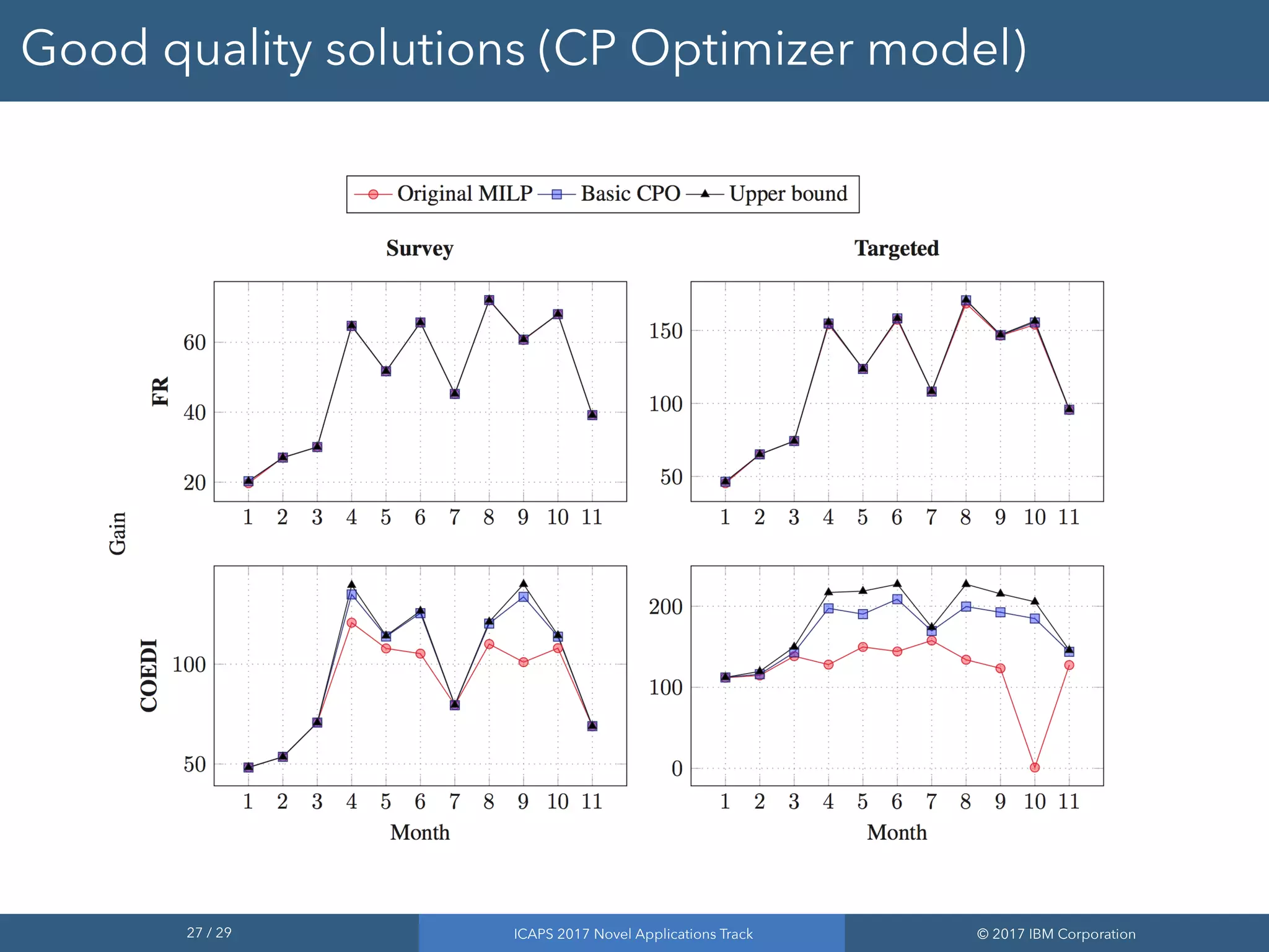
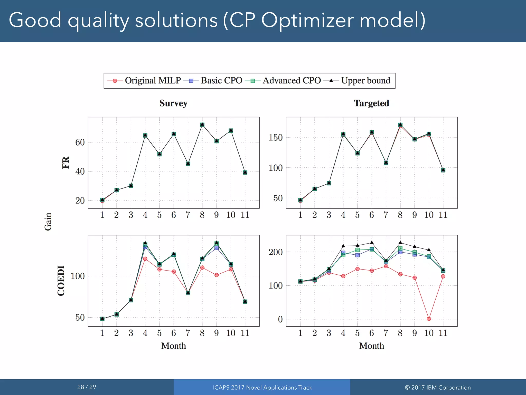


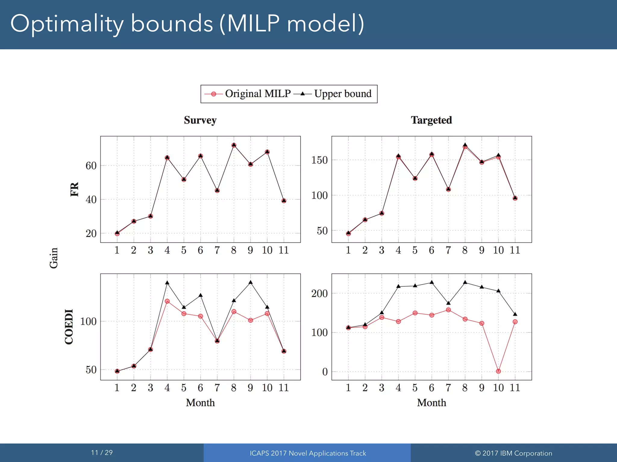
The document discusses the results of addressing the NASA satellite observation scheduling problem through improved optimization methods. It highlights the use of a mixed-integer linear programming (MILP) model and a constraint programming (CP) optimizer to achieve better quality solutions, with approximately 80% of instances yielding optimal or near-optimal solutions. The findings demonstrate the effectiveness of the CP optimizer in handling complex scheduling challenges and its adaptability for various observational scenarios.


![Vibe Coding vs. Spec-Driven Development [Free Meetup]](https://cdn.slidesharecdn.com/ss_thumbnails/vibecodingvsspecdrivendevelopment-251209105622-43f455e7-thumbnail.jpg?width=640&height=640&fit=bounds)