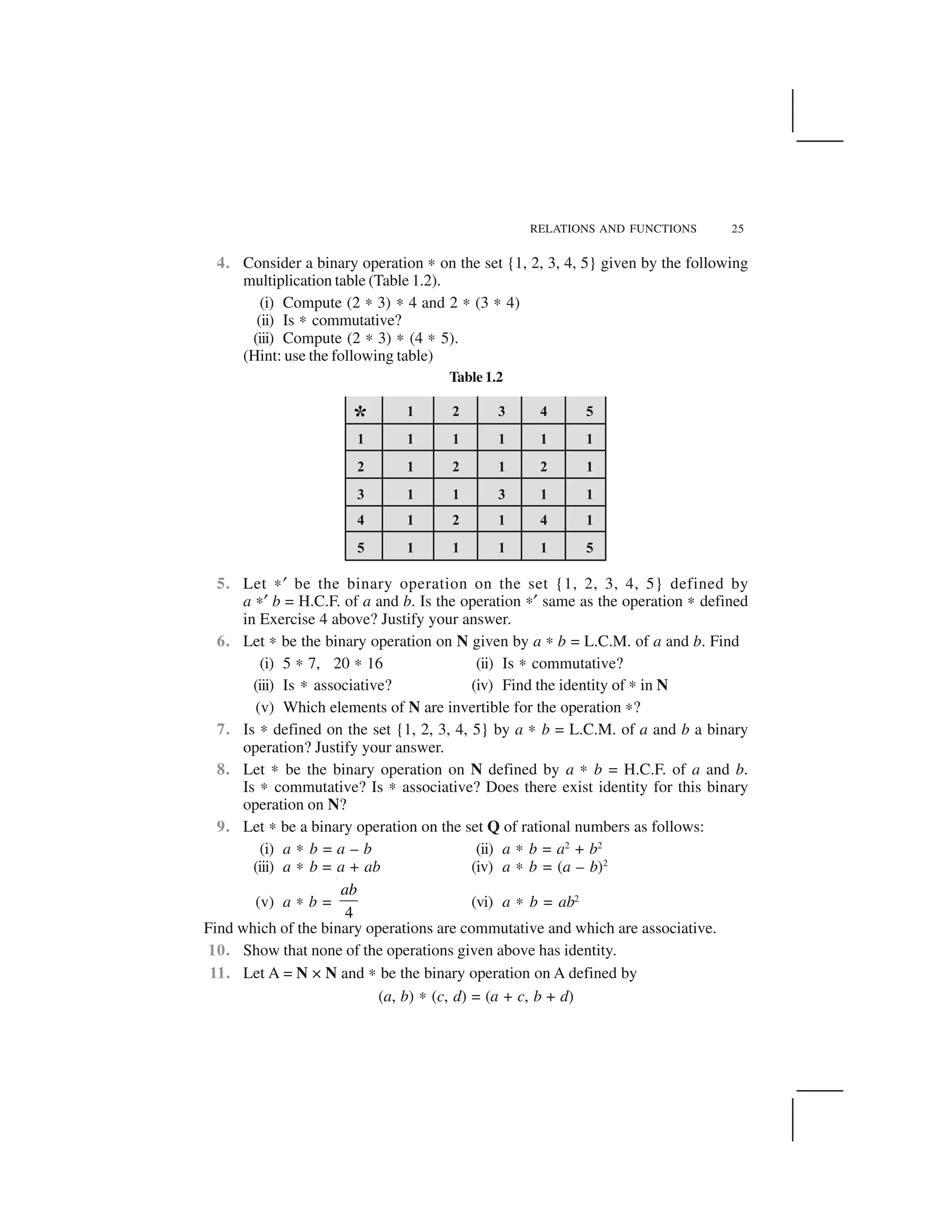
The document discusses types of relations. It defines empty relation, universal relation, reflexive relation, symmetric relation and transitive relation. An equivalence relation is a relation that is reflexive, symmetric and transitive. An equivalence relation partitions a set into mutually exclusive and exhaustive equivalence classes. Elements within an equivalence class are related to each other under the relation, while elements of different classes are not related. Examples of equivalence relations and their equivalence classes are provided.
![MATHEMATICS4
In Example 5, note that all even integers are related to zero, as (0, ± 2), (0, ± 4)
etc., lie in R and no odd integer is related to 0, as (0, ± 1), (0, ± 3) etc., do not lie in R.
Similarly, all odd integers are related to one and no even integer is related to one.
Therefore, the set E of all even integers and the set O of all odd integers are subsets of
Z satisfying following conditions:
(i) All elements of E are related to each other and all elements of O are related to
each other.
(ii) No element of E is related to any element of O and vice-versa.
(iii) E and O are disjoint and Z = E ✠ O.
The subset E is called the equivalence class containing zero and is denoted by
[0]. Similarly, O is the equivalence class containing 1 and is denoted by [1]. Note that
[0] ✡ [1], [0] = [2r] and [1] = [2r + 1], r ✂ Z. Infact, what we have seen above is true
for an arbitrary equivalence relation R in a set X. Given an arbitrary equivalence
relation R in an arbitrary set X, R divides X into mutually disjoint subsets Ai
called
partitions or subdivisions of X satisfying:
(i) all elements of Ai
are related to each other, for all i.
(ii) no element of Ai
is related to any element of Aj
, i ✡ j.
(iii) ✠ Aj
= X and Ai
☛ Aj
= ✄, i ✡ j.
The subsets Ai
are called equivalence classes. The interesting part of the situation
is that we can go reverse also. For example, consider a subdivision of the set Z given
by three mutually disjoint subsets A1
, A2
and A3
whose union is Z with
A1
= {x ✂ Z : x is a multiple of 3} = {..., – 6, – 3, 0, 3, 6, ...}
A2
= {x ✂ Z : x – 1 is a multiple of 3} = {..., – 5, – 2, 1, 4, 7, ...}
A3
= {x ✂ Z : x – 2 is a multiple of 3} = {..., – 4, – 1, 2, 5, 8, ...}
Define a relation R in Z given by R = {(a, b) : 3 divides a – b}. Following the
arguments similar to those used in Example 5, we can show that R is an equivalence
relation.Also,A1
coincides with the set of all integers in Z which are related to zero,A2
coincides with the set of all integers which are related to 1 and A3
coincides with the
set of all integers in Z which are related to 2. Thus, A1
= [0], A2
= [1] and A3
= [2].
In fact, A1
= [3r], A2
= [3r + 1] and A3
= [3r + 2], for all r ✂ Z.
Example 6 Let R be the relation defined in the set A = {1, 2, 3, 4, 5, 6, 7} by
R = {(a, b) : both a and b are either odd or even}. Show that R is an equivalence
relation. Further, show that all the elements of the subset {1, 3, 5, 7} are related to each
other and all the elements of the subset {2, 4, 6} are related to each other, but no
element of the subset {1, 3, 5, 7} is related to any element of the subset {2, 4, 6}.](https://image.slidesharecdn.com/ncert-class-12-mathematics-part-1-161112165946/75/Ncert-class-12-mathematics-part-1-7-2048.jpg)
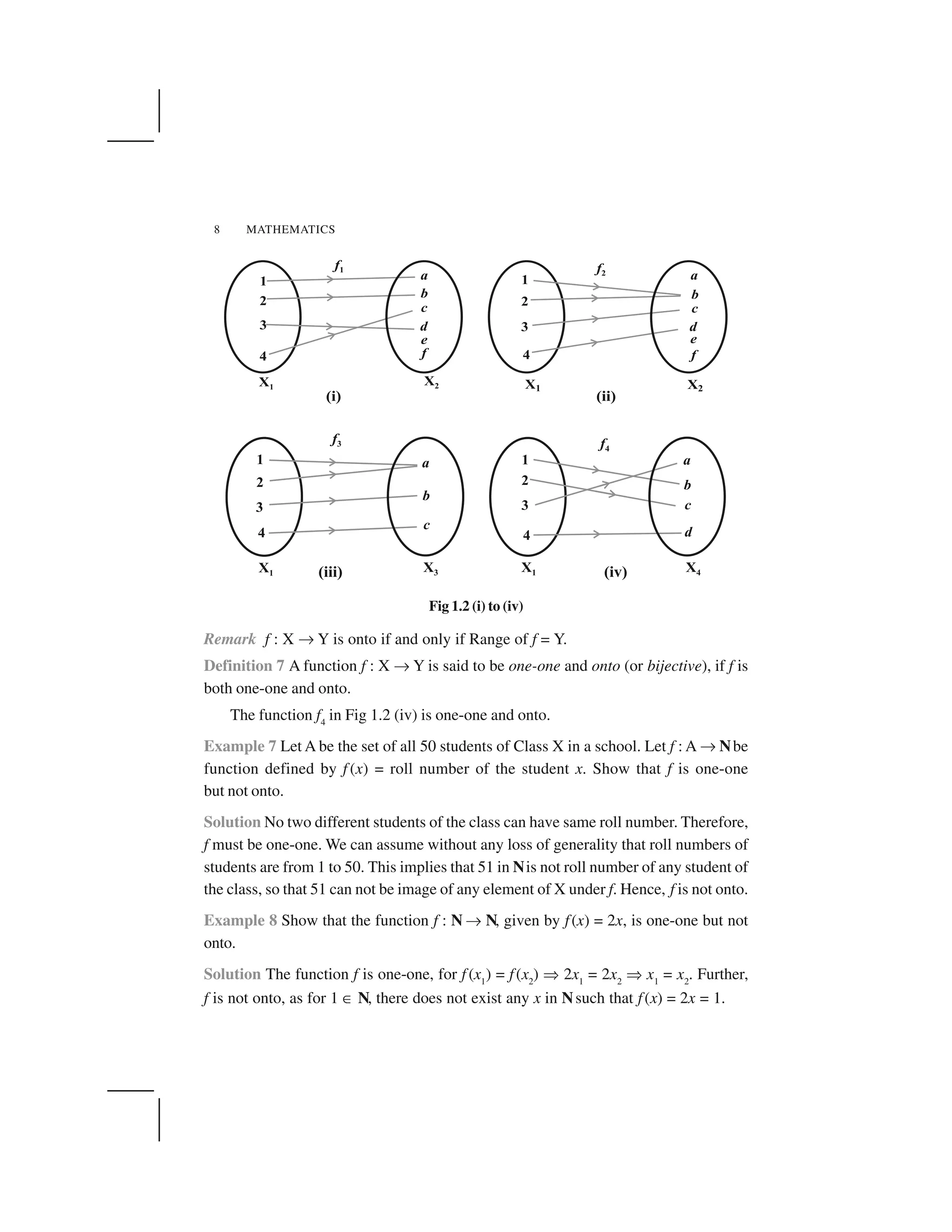
![MATHEMATICS10
Solution Suppose f (x1
) = f (x2
). Note that if x1
is odd and x2
is even, then we will have
x1
+ 1 = x2
– 1, i.e., x2
– x1
= 2 which is impossible. Similarly, the possibility of x1
being
even and x2
being odd can also be ruled out, using the similar argument. Therefore,
both x1
and x2
must be either odd or even. Suppose both x1
and x2
are odd. Then
f (x1
) = f (x2
) ✞x1
+ 1 = x2
+ 1 ✞x1
= x2
. Similarly, if both x1
and x2
are even, then also
f (x1
) = f (x2
) ✞ x1
– 1 = x2
– 1 ✞ x1
= x2
. Thus, f is one-one. Also, any odd number
2r + 1 in the co-domain N is the image of 2r + 2 in the domain N and any even number
2r in the co-domain N is the image of 2r – 1 in the domain N. Thus, f is onto.
Example 13 Show that an onto function f : {1, 2, 3} ✌{1, 2, 3} is always one-one.
Solution Suppose f is not one-one. Then there exists two elements, say 1 and 2 in the
domain whose image in the co-domain is same. Also, the image of 3 under f can be
only one element. Therefore, the range set can have at the most two elements of the
co-domain {1, 2, 3}, showing that f is not onto, a contradiction. Hence, f must be one-one.
Example 14 Show that a one-one function f : {1, 2, 3} ✌{1, 2, 3} must be onto.
Solution Since f is one-one, three elements of {1, 2, 3} must be taken to 3 different
elements of the co-domain {1, 2, 3} under f. Hence, f has to be onto.
Remark The results mentioned in Examples 13 and 14 are also true for an arbitrary
finite set X, i.e., a one-one function f : X ✌X is necessarily onto and an onto map
f : X ✌X is necessarily one-one, for every finite set X. In contrast to this, Examples 8
and 10 show that for an infinite set, this may not be true. In fact, this is a characteristic
difference between a finite and an infinite set.
EXERCISE 1.2
1. Show that the function f : R✍✍✍✍✍ ✌R✍✍✍✍✍ defined by f (x) =
1
x
is one-one and onto,
where R✍✍✍✍✍is the set of all non-zero real numbers. Is the result true, if the domain
R✍✍✍✍✍ is replaced by N with co-domain being same as R✍✍✍✍✍?
2. Check the injectivity and surjectivity of the following functions:
(i) f : N ✌N given by f(x) = x2
(ii) f : Z ✌Z given by f(x) = x2
(iii) f : R ✌R given by f(x) = x2
(iv) f : N ✌N given by f(x) = x3
(v) f : Z ✌Z given by f(x) = x3
3. Prove that the Greatest Integer Function f : R ✌R, given by f(x) = [x], is neither
one-one nor onto, where [x] denotes the greatest integer less than or equal to x.](https://image.slidesharecdn.com/ncert-class-12-mathematics-part-1-161112165946/75/Ncert-class-12-mathematics-part-1-13-2048.jpg)
![MATHEMATICS18
EXERCISE 1.3
1. Let f : {1, 3, 4} ✌ {1, 2, 5} and g : {1, 2, 5} ✌ {1, 3} be given by
f = {(1, 2), (3, 5), (4, 1)} and g = {(1, 3), (2, 3), (5, 1)}. Write down gof.
2. Let f, g and h be functions from R to R. Show that
(f + g)oh = foh + goh
(f . g)oh = (foh) . (goh)
3. Find gof and fog, if
(i) f (x) = | x | and g(x) = | 5x – 2 |
(ii) f (x) = 8x3
and g(x) =
1
3x .
4. If f (x) =
(4 3)
(6 4)
x
x
✁
,
2
3
x ✂ , show that fof (x) = x, for all
2
3
x✄ . What is the
inverse of f ?
5. State with reason whether following functions have inverse
(i) f : {1, 2, 3, 4} ✌ {10} with
f = {(1, 10), (2, 10), (3, 10), (4, 10)}
(ii) g : {5, 6, 7, 8} ✌ {1, 2, 3, 4} with
g = {(5, 4), (6, 3), (7, 4), (8, 2)}
(iii) h : {2, 3, 4, 5} ✌ {7, 9, 11, 13} with
h = {(2, 7), (3, 9), (4, 11), (5, 13)}
6. Show that f : [–1, 1] ✌ R, given by f (x) =
( 2)
x
x ☎
is one-one. Find the inverse
of the function f : [–1, 1] ✌ Range f.
(Hint: For y ✆ Range f, y = f (x) =
2
x
x ✝
, for some x in [–1, 1], i.e., x =
2
(1 )
y
y✞
)
7. Consider f : R ✌ R given by f (x) = 4x + 3. Show that f is invertible. Find the
inverse of f.
8. Consider f : R+
✌ [4, ✎) given by f (x) = x2
+ 4. Show that f is invertible with the
inverse f –1
of f given by f –1
(y) = 4y ✟ , where R+
is the set of all non-negative
real numbers.](https://image.slidesharecdn.com/ncert-class-12-mathematics-part-1-161112165946/75/Ncert-class-12-mathematics-part-1-21-2048.jpg)
![MATHEMATICS30
Define the relation R in P(X) as follows:
For subsets A, B in P(X), ARB if and only if A ✝B. Is R an equivalence relation
on P(X)? Justify your answer.
9. Given a non-empty set X, consider the binary operation ✍: P(X) × P(X) ✌P(X)
given by A ✍ B = A ☛ B A, B in P(X), where P(X) is the power set of X.
Show that X is the identity element for this operation and X is the only invertible
element in P(X) with respect to the operation ✍.
10. Find the number of all onto functions from the set {1, 2, 3, ... , n} to itself.
11. Let S = {a, b, c} and T = {1, 2, 3}. Find F–1
of the following functions F from S
to T, if it exists.
(i) F = {(a, 3), (b, 2), (c, 1)} (ii) F = {(a, 2), (b, 1), (c, 1)}
12. Consider the binary operations ✍ : R × R ✌ R and o : R × R ✌ R defined as
a ✍b = |a – b| and a o b = a, a, b ✂ R. Show that ✍ is commutative but not
associative, o is associative but not commutative. Further, show that a, b, c ✂R,
a ✍ (b o c) = (a ✍ b) o (a ✍b). [If it is so, we say that the operation ✍ distributes
over the operation o]. Does o distribute over ✍? Justify your answer.
13. Given a non-empty set X, let ✍ : P(X) × P(X) ✌ P(X) be defined as
A * B = (A – B) ✠ (B – A), A, B ✂ P(X). Show that the empty set ✄ is the
identity for the operation ✍ and all the elements A of P(X) are invertible with
A–1
= A. (Hint : (A – ✄) ✠ (✄ – A) = A and (A – A) ✠ (A – A) = A ✍ A = ✄).
14. Define a binary operation ✍ on the set {0, 1, 2, 3, 4, 5} as
, if 6
6 if 6
a b a b
a b
a b a b
✁ ✁ ☎✆✞ ✟ ✡ ✁ ☞ ✁ ✎✏
Show that zero is the identity for this operation and each element a of the set is
invertible with 6 – a being the inverse of a.
15. Let A = {– 1, 0, 1, 2}, B = {– 4, – 2, 0, 2} and f, g : A ✌ B be functions defined
by f (x) = x2
– x, x ✂ A and
1
( ) 2 1,
2
g x x✑ ✒ ✒ x ✂ A. Are f and g equal?
Justify your answer. (Hint: One may note that two functions f : A ✌ B and
g : A ✌ B such that f (a) = g(a) a ✂ A, are called equal functions).
16. LetA= {1, 2, 3}. Then number of relations containing (1, 2) and (1, 3) which are
reflexive and symmetric but not transitive is
(A) 1 (B) 2 (C) 3 (D) 4
17. Let A = {1, 2, 3}. Then number of equivalence relations containing (1, 2) is
(A) 1 (B) 2 (C) 3 (D) 4](https://image.slidesharecdn.com/ncert-class-12-mathematics-part-1-161112165946/75/Ncert-class-12-mathematics-part-1-33-2048.jpg)
![RELATIONS AND FUNCTIONS 31
18. Let f : R ✌ R be the Signum Function defined as
1, 0
( ) 0, 0
1, 0
x
f x x
x
✁
✂
✄ ✄☎
✂✆ ✝✞
and g : R ✌ R be the Greatest Integer Function given by g(x) = [x], where [x] is
greatest integer less than or equal to x. Then, does fog and gof coincide in (0, 1]?
19. Number of binary operations on the set {a, b} are
(A) 10 (B) 16 (C) 20 (D ) 8
Summary
In this chapter, we studied different types of relations and equivalence relation,
composition of functions, invertible functions and binary operations. The main features
of this chapter are as follows:
✟ Empty relation is the relation R in X given by R = ✠ ✡ X × X.
✟ Universal relation is the relation R in X given by R = X × X.
✟ Reflexive relation R in X is a relation with (a, a) ☛ R ☞ a ☛ X.
✟ Symmetric relation R in X is a relation satisfying (a, b) ☛ R implies (b, a) ☛ R.
✟ Transitive relation R in X is a relation satisfying (a, b) ☛ R and (b, c) ☛ R
implies that (a, c) ☛ R.
✟ Equivalence relation R in X is a relation which is reflexive, symmetric and
transitive.
✟ Equivalence class [a] containing a ☛ X for an equivalence relation R in X is
the subset of X containing all elements b related to a.
✟ A function f : X ✌ Y is one-one (or injective) if
f (x1
) = f(x2
) ✍ x1
= x2 ☞ x1
, x2
☛ X.
✟ A function f : X ✌ Y is onto (or surjective) if given any y ☛ Y, ✏ x ☛ X such
that f (x) = y.
✟ A function f : X ✌ Y is one-one and onto (or bijective), if f is both one-one
and onto.
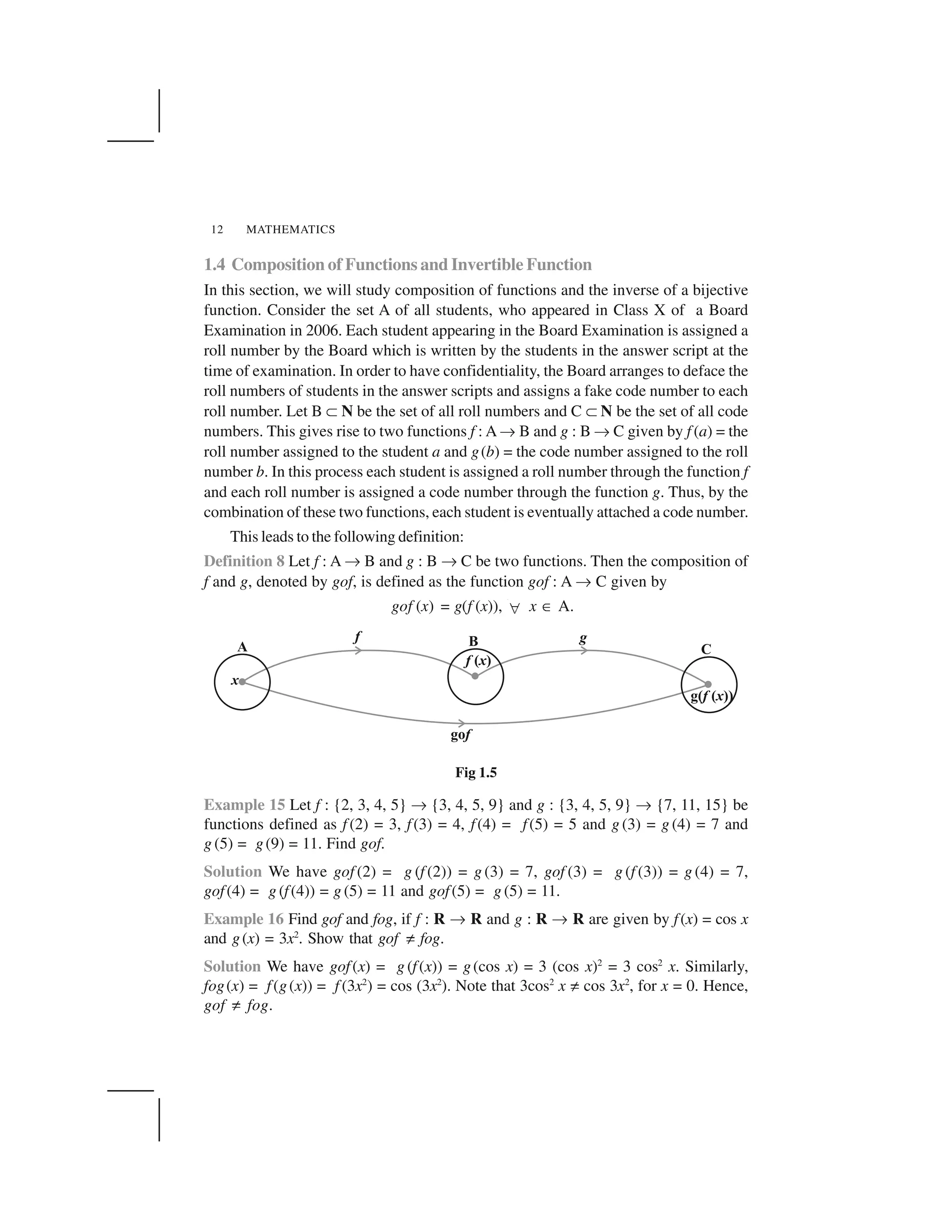
✟ The composition of functions f : A ✌ B and g : B ✌ C is the function
gof : A ✌ C given by gof (x) = g(f (x))☞ x ☛ A.
✟ A function f : X ✌ Y is invertible if ✏ g : Y ✌ X such that gof = IX
and
fog = IY
.
✟ A function f : X ✌ Y is invertible if and only if f is one-one and onto.](https://image.slidesharecdn.com/ncert-class-12-mathematics-part-1-161112165946/75/Ncert-class-12-mathematics-part-1-34-2048.jpg)
![Mathematics, in general, is fundamentally the science of
self-evident things. — FELIX KLEIN
2.1 Introduction
In Chapter 1, we have studied that the inverse of a function
f, denoted by f –1
, exists if f is one-one and onto. There are
many functions which are not one-one, onto or both and
hence we can not talk of their inverses. In Class XI, we
studied that trigonometric functions are not one-one and
onto over their natural domains and ranges and hence their
inverses do not exist. In this chapter, we shall study about
the restrictions on domains and ranges of trigonometric
functions which ensure the existence of their inverses and
observe their behaviour through graphical representations.
Besides, some elementary properties will also be discussed.
The inverse trigonometric functions play an important
role in calculus for they serve to define many integrals.
The concepts of inverse trigonometric functions is also used in science and engineering.
2.2 Basic Concepts
In Class XI, we have studied trigonometric functions, which are defined as follows:
sine function, i.e., sine : R ✂[– 1, 1]
cosine function, i.e., cos : R ✂[– 1, 1]
tangent function, i.e., tan : R – { x : x = (2n + 1)
2
✁, n ✥Z} ✂R
cotangent function, i.e., cot : R – { x : x = n☎, n ✥Z} ✂R
secant function, i.e., sec : R – { x : x = (2n + 1)
2
✁ , n ✥Z} ✂R – (– 1, 1)
cosecant function, i.e., cosec : R – { x : x = n☎, n ✥Z} ✂R – (– 1, 1)
Chapter 2
INVERSE TRIGONOMETRIC
FUNCTIONS
Arya Bhatta
(476-550 A. D.)](https://image.slidesharecdn.com/ncert-class-12-mathematics-part-1-161112165946/75/Ncert-class-12-mathematics-part-1-36-2048.jpg)
![34 MATHEMATICS
We have also learnt in Chapter 1 that if f : X✂Y such that f (x) = y is one-one and
onto, then we can define a unique function g : Y✂X such that g(y) = x, where x ✄ X
and y = f (x), y ✄ Y. Here, the domain of g = range of f and the range of g = domain
of f. The function g is called the inverse of f and is denoted by f –1
. Further, g is also
one-one and onto and inverse of g is f. Thus, g–1
= (f –1
)–1
= f. We also have
(f –1
o f ) (x) = f –1
(f (x)) = f –1
(y) = x
and (f o f –1
) (y) = f (f –1
(y)) = f (x) = y
Since the domain of sine function is the set of all real numbers and range is the
closed interval [–1, 1]. If we restrict its domain to ,
2 2
✁ ✁☎ ✆
✝ ✞✟ ✠
, then it becomes one-one
and onto with range [– 1, 1]. Actually, sine function restricted to any of the intervals
3 –
,
2 2
✡ ☛ ☛☞ ✌
✍ ✎✏ ✑
, ,
2 2
✡☛ ☛☞ ✌
✍ ✎✏ ✑
,
3
,
2 2
✒ ✒✓ ✔
✕ ✖✗ ✘
etc., is one-one and its range is [–1, 1]. We can,
therefore, define the inverse of sine function in each of these intervals. We denote the
inverse of sine function by sin–1
(arc sine function). Thus, sin–1
is a function whose
domain is [– 1, 1] and range could be any of the intervals
3
,
2 2
✙ ✒ ✙✒✓ ✔
✕ ✖✗ ✘
, ,
2 2
✙✒ ✒✓ ✔
✕ ✖✗ ✘
or
3
,
2 2
☛ ☛☞ ✌
✍ ✎✏ ✑
, and so on. Corresponding to each such interval, we get a branch of the
function sin–1
. The branch with range ,
2 2
✙✒ ✒✓ ✔
✕ ✖✗ ✘
is called the principal value branch,
whereas other intervals as range give different branches of sin–1
. When we refer
to the function sin–1
, we take it as the function whose domain is [–1, 1] and range is
,
2 2
✙✒ ✒✓ ✔
✕ ✖✗ ✘
. We write sin–1
: [–1, 1] ✂ ,
2 2
✙✒ ✒✓ ✔
✕ ✖✗ ✘
From the definition of the inverse functions, it follows that sin (sin–1
x) = x
if – 1 ✚ x ✚ 1 and sin–1
(sin x) = x if
2 2
x
✛ ✛
✜ ✢ ✢ . In other words, if y = sin–1
x, then
sin y = x.
Remarks
(i) We know from Chapter 1, that if y = f(x) is an invertible function, then x = f –1
(y).
Thus, the graph of sin–1
function can be obtained from the graph of original
function by interchanging x and y axes, i.e., if (a, b) is a point on the graph of
sine function, then (b, a) becomes the corresponding point on the graph of inverse](https://image.slidesharecdn.com/ncert-class-12-mathematics-part-1-161112165946/75/Ncert-class-12-mathematics-part-1-37-2048.jpg)
![INVERSE TRIGONOMETRIC FUNCTIONS 35
of sine function. Thus, the graph of the function y = sin–1
x can be obtained from
the graph of y = sin x by interchanging x and y axes. The graphs of y = sin x and
y = sin–1
x are as given in Fig 2.1 (i), (ii), (iii). The dark portion of the graph of
y = sin–1
x represent the principal value branch.
(ii) It can be shown that the graph of an inverse function can be obtained from the
corresponding graph of original function as a mirror image (i.e., reflection) along
the line y = x. This can be visualised by looking the graphs of y = sin x and
y = sin–1
x as given in the same axes (Fig 2.1 (iii)).
Like sine function, the cosine function is a function whose domain is the set of all
real numbers and range is the set [–1, 1]. If we restrict the domain of cosine function
to [0, ☎], then it becomes one-one and onto with range [–1, 1].Actually, cosine function
Fig 2.1 (ii) Fig 2.1 (iii)
Fig 2.1 (i)](https://image.slidesharecdn.com/ncert-class-12-mathematics-part-1-161112165946/75/Ncert-class-12-mathematics-part-1-38-2048.jpg)
![36 MATHEMATICS
restricted to any of the intervals [– ☎, 0], [0,☎], [☎, 2☎] etc., is bijective with range as
[–1, 1]. We can, therefore, define the inverse of cosine function in each of these
intervals. We denote the inverse of the cosine function by cos–1
(arc cosine function).
Thus, cos–1
is a function whose domain is [–1, 1] and range
could be any of the intervals [–☎, 0], [0, ☎], [☎, 2☎] etc.
Corresponding to each such interval, we get a branch of the
function cos–1
. The branch with range [0,☎] is called theprincipal
value branch of the function cos–1
. We write
cos–1
: [–1, 1] ✂ [0, ☎].
The graph of the function given by y = cos–1
x can be drawn
in the same way as discussed about the graph of y = sin–1
x. The
graphs of y = cos x and y = cos–1
x are given in Fig 2.2 (i) and (ii).
Fig 2.2 (ii)
Let us now discuss cosec–1
x and sec–1
x as follows:
Since, cosec x =
1
sin x
, the domain of the cosec function is the set {x : x ✄ R and
x ✝ n☎, n ✄ Z} and the range is the set {y : y ✄ R, y ✞ 1 or y ✆ –1} i.e., the set
R – (–1, 1). It means that y = cosec x assumes all real values except –1 < y < 1 and is
not defined for integral multiple of ☎. If we restrict the domain of cosec function to
,
2 2
✁ ✟
✠✡ ☛☞ ✌
–{0},thenitisonetooneand onto with itsrangeas thesetR–(– 1,1).Actually,
cosec function restricted to any of the intervals
3
, { }
2 2
✍ ✎ ✍✎✏ ✑
✍ ✍✎✒ ✓✔ ✕
, ,
2 2
✍✎ ✎✏ ✑
✒ ✓✔ ✕
– {0},
3
, { }
2 2
✁ ✟
✠ ✡ ☛☞ ✌
etc., is bijective and its range is the set of all real numbers R – (–1, 1).
Fig 2.2 (i)](https://image.slidesharecdn.com/ncert-class-12-mathematics-part-1-161112165946/75/Ncert-class-12-mathematics-part-1-39-2048.jpg)
![INVERSE TRIGONOMETRIC FUNCTIONS 37
Thus cosec–1
can be defined as a function whose domain is R – (–1, 1) and range could
be any of the intervals , {0}
2 2
✁ ✁✂ ✄
☎ ✆✝ ✞
,
3
, { }
2 2
✁ ✁✂ ✄
✁☎ ✆✝ ✞
,
3
, { }
2 2
✟ ✟✠ ✡
☛ ✟☞ ✌✍ ✎
etc. The
function corresponding to the range , {0}
2 2
✁ ✁✂ ✄ ☎ ✆✝ ✞
is called the principal value branch
of cosec–1
. We thus have principal branch as
cosec–1
: R – (–1, 1) ✏ , {0}
2 2
✁ ✁✂ ✄ ☎ ✆✝ ✞
The graphs of y = cosec x and y = cosec–1
x are given in Fig 2.3 (i), (ii).
Also, since sec x =
1
cos x
, the domain of y = sec x is the set R – {x : x = (2n + 1)
2
✑
,
n ✒ Z} and range is the set R – (–1, 1). It means that sec (secant function) assumes
all real values except –1 < y < 1 and is not defined for odd multiples of
2
✑
. If we
restrict the domain of secant function to [0, ✓] – {
2
✑
}, then it is one-one and onto with
Fig 2.3 (i) Fig 2.3 (ii)](https://image.slidesharecdn.com/ncert-class-12-mathematics-part-1-161112165946/75/Ncert-class-12-mathematics-part-1-40-2048.jpg)
![38 MATHEMATICS
its range as the set R – (–1, 1). Actually, secant function restricted to any of the
intervals [–☎, 0] – {
2
✁
}, [0, ] –
2
✂✄ ✆
✂ ✝ ✞
✟ ✠
, [☎, 2☎] – {
3
2
✁
} etc., is bijective and its range
is R – {–1, 1}. Thus sec–1
can be defined as a function whose domain is R– (–1, 1) and
range could be any of the intervals [– ☎, 0] – {
2
✁
}, [0, ☎] – {
2
✁
}, [☎, 2☎] – {
3
2
✁
} etc.
Corresponding to each of these intervals, we get different branches of the function sec–1
.
The branch with range [0, ☎] – {
2
✁
} is called the principal value branch of the
function sec–1
. We thus have
sec–1
: R – (–1,1) ✡ [0, ☎] – {
2
✁
}
The graphs of the functions y = sec x and y = sec-1
x are given in Fig 2.4 (i), (ii).
Finally, we now discuss tan–1
and cot–1
We know that the domain of the tan function (tangent function) is the set
{x : x ☛ R and x ☞ (2n +1)
2
✁
, n ☛ Z} and the range is R. It means that tan function
is not defined for odd multiples of
2
✁
. If we restrict the domain of tangent function to
Fig 2.4 (i) Fig 2.4 (ii)](https://image.slidesharecdn.com/ncert-class-12-mathematics-part-1-161112165946/75/Ncert-class-12-mathematics-part-1-41-2048.jpg)
![40 MATHEMATICS
intervals (–☎, 0), (0, ☎), (☎, 2☎) etc. These intervals give different branches of the
function cot–1
. The function with range (0, ☎) is called the principal value branch of
the function cot–1
. We thus have
cot–1
: R ✂ (0, ☎)
The graphs of y = cot x and y = cot–1
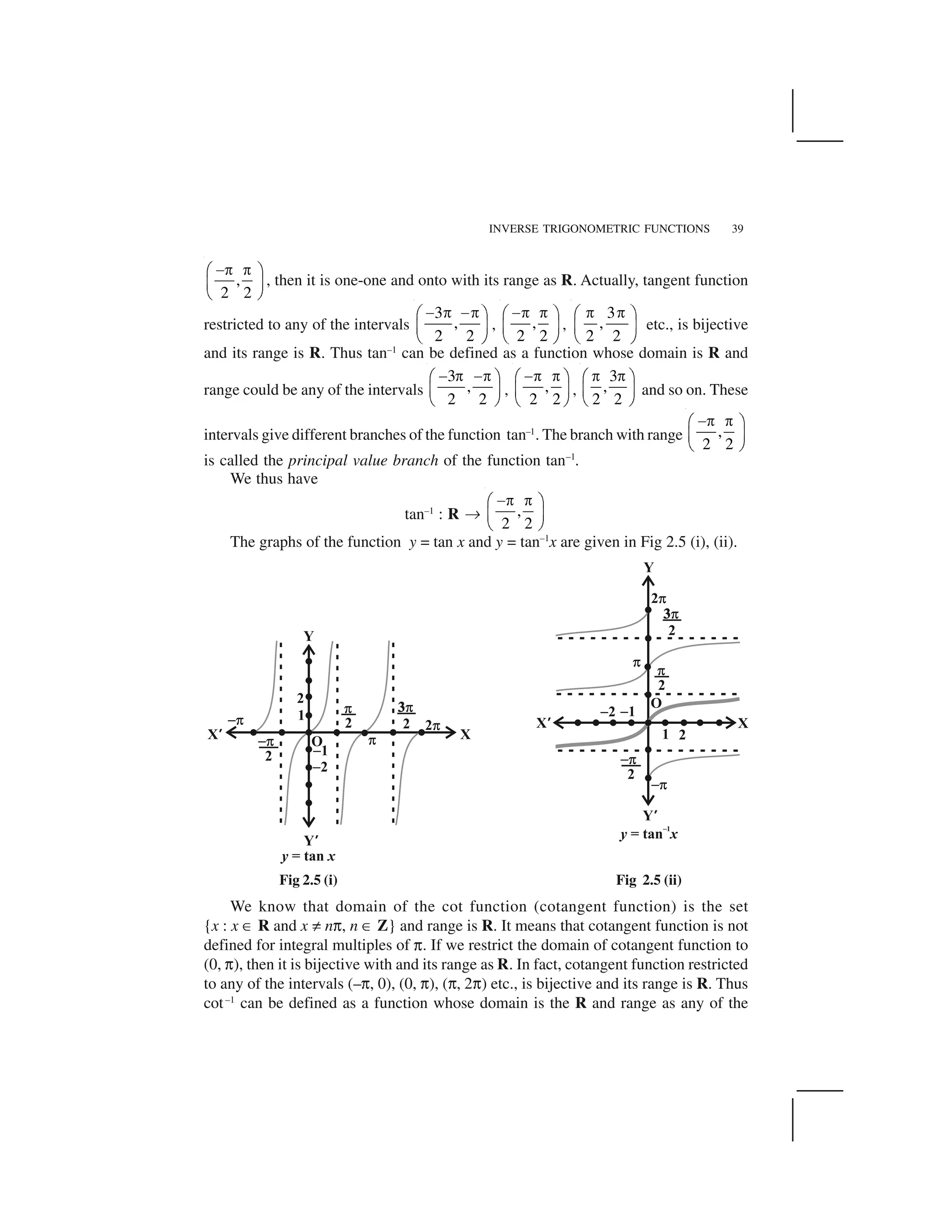
x are given in Fig 2.6 (i), (ii).
Fig 2.6 (i) Fig 2.6 (ii)
The following table gives the inverse trigonometric function (principal value
branches) along with their domains and ranges.
sin–1
: [–1, 1] ✂ ,
2 2
✁ ✄
✆✝ ✞✟ ✠
cos–1
: [–1, 1] ✂ [0, ☎]
cosec–1
: R – (–1,1) ✂ ,
2 2
✡ ✡☛ ☞
✌✍ ✎✏ ✑
– {0}
sec–1
: R – (–1, 1) ✂ [0, ☎] – { }
2
✒
tan–1
: R ✂ ,
2 2
✌✡ ✡✓ ✔
✕ ✖
✗ ✘
cot–1
: R ✂ (0, ☎)](https://image.slidesharecdn.com/ncert-class-12-mathematics-part-1-161112165946/75/Ncert-class-12-mathematics-part-1-43-2048.jpg)
![42 MATHEMATICS
7. sec–1
2
3
✁
✂ ✄
☎ ✆
8. cot–1
( 3) 9. cos–1
1
2
✁
✝✂ ✄
☎ ✆
10. cosec–1
( 2✞ )
Find the values of the following:
11. tan–1
(1) + cos–1
1
2
✟ ✠
✡☛ ☞
✌ ✍
+ sin–1
1
2
✎ ✏
✑✒ ✓
✔ ✕
12. cos–1
1
2
✟ ✠
☛ ☞
✌ ✍
+ 2 sin–1
1
2
✎ ✏
✒ ✓
✔ ✕
13. If sin–1
x = y, then
(A) 0 ✖ y ✖ ✗ (B)
2 2
y
✘ ✘
✙ ✚ ✚
(C) 0 < y < ✗ (D)
2 2
y
✛ ✛
✜ ✢ ✢
14. tan–1
✣ ✤
1
3 sec 2✥
✦ ✦ is equal to
(A) ✗ (B)
3
✘
✙ (C)
3
✘
(D)
2
3
✘
2.3 Properties of Inverse Trigonometric Functions
In this section, we shall prove some important properties of inverse trigonometric
functions. It may be mentioned here that these results are valid within the principal
value branches of the corresponding inverse trigonometric functions and wherever
they are defined. Some results may not be valid for all values of the domains of inverse
trigonometric functions. In fact, they will be valid only for some values of x for which
inverse trigonometric functions are defined. We will not go into the details of these
values of x in the domain as this discussion goes beyond the scope of this text book.
Let us recall that if y = sin–1
x, then x = sin y and if x = sin y, then y = sin–1
x. This is
equivalent to
sin (sin–1
x) = x, x ✧ [– 1, 1] and sin–1
(sin x) = x, x ✧ ,
2 2
★ ★✩ ✪
✫
✬ ✭
✮ ✯
Same is true for other five inverse trigonometric functions as well. We now prove
some properties of inverse trigonometric functions.
1. (i) sin–1
1
x
= cosec–1
x, x ✰✰ 1 or x ✖✖✖✖ – 1
(ii) cos–1
1
x
= sec–1
x, x ✰✰ 1 or x ✖ – 1](https://image.slidesharecdn.com/ncert-class-12-mathematics-part-1-161112165946/75/Ncert-class-12-mathematics-part-1-45-2048.jpg)
![INVERSE TRIGONOMETRIC FUNCTIONS 43
(iii) tan–1
1
x
= cot–1
x, x > 0
To prove the first result, we put cosec–1
x = y, i.e., x = cosec y
Therefore
1
x
= sin y
Hence sin–1
1
x
= y
or sin–1
1
x
= cosec–1
x
Similarly, we can prove the other parts.
2. (i) sin–1
(–x) = – sin–1
x, x ✄ [– 1, 1]
(ii) tan–1
(–x) = – tan–1
x, x ✄ R
(iii) cosec–1
(–x) = – cosec–1
x, | x | ✞ 1
Let sin–1
(–x) = y, i.e., –x = sin y so that x = – sin y, i.e., x = sin (–y).
Hence sin–1
x = – y = – sin–1
(–x)
Therefore sin–1
(–x) = – sin–1
x
Similarly, we can prove the other parts.
3. (i) cos–1
(–x) = ☎☎ – cos–1
x, x ✄✄ [– 1, 1]
(ii) sec–1
(–x) = ☎ – sec–1
x, | x | ✞ 1
(iii) cot–1
(–x) = ☎ – cot–1
x, x ✄ R
Let cos–1
(–x) = y i.e., – x = cos y so that x = – cos y = cos (☎ – y)
Therefore cos–1
x = ☎ – y = ☎ – cos–1
(–x)
Hence cos–1
(–x) = ☎ – cos–1
x
Similarly, we can prove the other parts.
4. (i) sin–1
x + cos–1
x =
2
, x ✄✄✄✄ [– 1, 1]
(ii) tan–1
x + cot–1
x =
2
, x ✄✄ R
(iii) cosec–1
x + sec–1
x =
2
, | x | ✞✞✞✞ 1
Let sin–1
x = y. Then x = sin y = cos
2
y
✁ ✂
✆✝ ✟
✠ ✡
Therefore cos–1
x =
2
y
☛
☞ =
–1
sin
2
x
☛
☞](https://image.slidesharecdn.com/ncert-class-12-mathematics-part-1-161112165946/75/Ncert-class-12-mathematics-part-1-46-2048.jpg)
![52 MATHEMATICS
Prove that
9.
–1 –11 1
tan cos
2 1
x
x
x
✁ ✂
✄ ☎ ✆✝ ✞✟
, x ✠ [0, 1]
10. –1 1 sin 1 sin
cot
21 sin 1 sin
x x x
x x
✡ ☛☞ ☞ ✌
✍✎ ✏✎ ✏☞ ✌ ✌✑ ✒
, 0,
4
x
✓✔ ✕✖✗ ✘
✙ ✚
11.
–1 –11 1 1
tan cos
4 21 1
x x
x
x x
✡ ☛☞ ✌ ✌ ✛
✍ ✌✎ ✏✎ ✏☞ ☞ ✌✑ ✒
,
1
1
2
x✜ ✢ ✢ [Hint: Put x = cos 2✣]
12.
1 19 9 1 9 2 2
sin sin
8 4 3 4 3
✤ ✤✓
✜ ✥
Solve the following equations:
13. 2tan–1
(cos x) = tan–1
(2 cosec x) 14.
–1 –11 1
tan tan ,( 0)
1 2
x
x x
x
✦
✧ ★
✩
15. sin (tan–1
x), |x| < 1 is equal to
(A) 2
1
x
x✪
(B) 2
1
1 x✪
(C) 2
1
1 x✫
(D) 2
1
x
x✫
16. sin–1
(1 – x) – 2 sin–1
x =
2
✬
, then x is equal to
(A) 0,
1
2
(B) 1,
1
2
(C) 0 (D)
1
2
17.
1 1
tan tan
x x y
y x y
✭ ✭ ✪✮ ✯ ✪✰ ✱ ✫✲ ✳
is equal to
(A)
2
✬
(B)
3
✬
(C)
4
✬
(D)
3
4
✦ ✬](https://image.slidesharecdn.com/ncert-class-12-mathematics-part-1-161112165946/75/Ncert-class-12-mathematics-part-1-55-2048.jpg)
![INVERSE TRIGONOMETRIC FUNCTIONS 53
Summary
The domains and ranges (principal value branches) of inverse trigonometric
functions are given in the following table:
Functions Domain Range
(Principal Value Branches)
y = sin–1
x [–1, 1] ,
2 2
✁✂ ✂✄ ☎✆ ✝✞ ✟
y = cos–1
x [–1, 1] [0, ✠]
y = cosec–1
x R – (–1,1) ,
2 2
✡☛ ☛☞ ✌
✍ ✎✏ ✑ – {0}
y = sec–1
x R – (–1, 1) [0, ✠] – { }
2
✒
y = tan–1
x R ,
2 2
✂ ✂✓ ✔✁✕ ✖✗ ✘
y = cot–1
x R (0, ✠)
sin–1
x should not be confused with (sin x)–1
. In fact (sin x)–1
=
1
sin x
and
similarly for other trigonometric functions.
The value of an inverse trigonometric functions which lies in its principal
value branch is called the principal value of that inverse trigonometric
functions.
For suitable values of domain, we have
y = sin–1
x ✙ x = sin y x = sin y ✙ y = sin–1
x
sin (sin–1
x) = x sin–1
(sin x) = x
sin–1
1
x
= cosec–1
x cos–1
(–x) = ✠ – cos–1
x
cos–1
1
x
= sec–1
x cot–1
(–x) = ✠ – cot–1
x
tan–1
1
x
= cot–1
x sec–1
(–x) = ✠ – sec–1
x](https://image.slidesharecdn.com/ncert-class-12-mathematics-part-1-161112165946/75/Ncert-class-12-mathematics-part-1-56-2048.jpg)
![The essence of Mathematics lies in its freedom. — CANTOR
3.1 Introduction
The knowledge of matrices is necessary in various branches of mathematics. Matrices
are one of the most powerful tools in mathematics. This mathematical tool simplifies
our work to a great extent when compared with other straight forward methods. The
evolution of concept of matrices is the result of an attempt to obtain compact and
simple methods of solving system of linear equations. Matrices are not only used as a
representation of the coefficients in system of linear equations, but utility of matrices
far exceeds that use. Matrix notation and operations are used in electronic spreadsheet
programs for personal computer, which in turn is used in different areas of business
and science like budgeting, sales projection, cost estimation, analysing the results of an
experiment etc. Also, many physical operations such as magnification, rotation and
reflection through a plane can be represented mathematically by matrices. Matrices
are also used in cryptography.This mathematical tool is not only used in certain branches
of sciences, but also in genetics, economics, sociology, modern psychology and industrial
management.
In this chapter, we shall find it interesting to become acquainted with the
fundamentals of matrix and matrix algebra.
3.2 Matrix
Suppose we wish to express the information that Radha has 15 notebooks. We may
express it as [15] with the understanding that the number inside [ ] is the number of
notebooks that Radha has. Now, if we have to express that Radha has 15 notebooks
and 6 pens. We may express it as [15 6] with the understanding that first number
inside [ ] is the number of notebooks while the other one is the number of pens possessed
by Radha. Let us now suppose that we wish to express the information of possession
Chapter 3
MATRICES](https://image.slidesharecdn.com/ncert-class-12-mathematics-part-1-161112165946/75/Ncert-class-12-mathematics-part-1-59-2048.jpg)
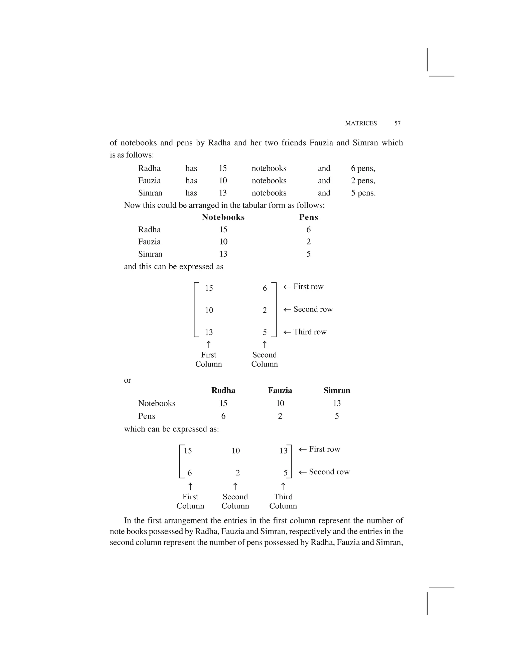
![58 MATHEMATICS
respectively. Similarly, in the second arrangement, the entries in the first row represent
the number of notebooks possessed by Radha, Fauzia and Simran, respectively. The
entries in the second row represent the number of pens possessed by Radha, Fauzia
and Simran, respectively. An arrangement or display of the above kind is called a
matrix. Formally, we define matrix as:
Definition 1 A matrix is an ordered rectangular array of numbers or functions. The
numbers or functions are called the elements or the entries of the matrix.
We denote matrices by capital letters. The following are some examples of matrices:
5– 2
A 0 5
3 6
✁
✂ ✄
☎ ✂ ✄
✂ ✄
✆ ✝
,
1
2 3
2
B 3.5 –1 2
5
3 5
7
i
✞ ✟
✠ ✡
☛ ☞
☛ ☞
✌ ☛ ☞
☛ ☞
☛ ☞
✍ ✎
,
3
1 3
C
cos tansin 2
x x
x xx
✏ ✑✒
✓ ✔ ✕
✒✖ ✗
In the above examples, the horizontal lines of elements are said to constitute, rows
of the matrix and the vertical lines of elements are said to constitute, columns of the
matrix. Thus A has 3 rows and 2 columns, B has 3 rows and 3 columns while C has 2
rows and 3 columns.
3.2.1 Order of a matrix
Amatrix having m rows and n columns is called a matrix of order m × n or simply m × n
matrix (read as an m by n matrix). So referring to the above examples of matrices, we
have A as 3 × 2 matrix, B as 3 × 3 matrix and C as 2 × 3 matrix. We observe thatA has
3 × 2 = 6 elements, B and C have 9 and 6 elements, respectively.
In general, an m × n matrix has the following rectangular array:
or A = [aij
]m × n
, 1✘ i ✘ m, 1✘ j ✘ n i, j ✙ N
Thus the ith
row consists of the elements ai1
, ai2
, ai3
,..., ain
, while the jth
column
consists of the elements a1j
, a2j
, a3j
,..., amj
,
In general aij
, is an element lying in the ith
row and jth
column. We can also call
it as the (i, j)th
element of A. The number of elements in an m × n matrix will be
equal to mn.](https://image.slidesharecdn.com/ncert-class-12-mathematics-part-1-161112165946/75/Ncert-class-12-mathematics-part-1-61-2048.jpg)
![MATRICES 59
Note In this chapter
1. We shall follow the notation, namelyA= [aij
]m × n
to indicate thatAis a matrix
of order m × n.
2. We shall consider only those matrices whose elements are real numbers or
functions taking real values.
We can also represent any point (x, y) in a plane by a matrix (column or row) as
x
y
✁ ✂✄ ☎✆ ✝(or [x, y]). For example point P(0, 1) as a matrix representation may be given as
0
P
1
✞ ✟✠✡ ☛☞ ✌or [0 1].
Observe that in this way we can also express the vertices of a closed rectilinear
figure in the form of a matrix. For example, consider a quadrilateral ABCD with vertices
A (1, 0), B (3, 2), C (1, 3), D (–1, 2).
Now, quadrilateral ABCD in the matrix form, can be represented as
2 4
A B C D
1 3 1 1
X
0 2 3 2 ✍
✎✏ ✑✒✓ ✔✕ ✖ or
4 2
A 1 0
B 3 2
Y
C 1 3
D 1 2 ✗
✘ ✙✚ ✛✚ ✛✜ ✚ ✛✚ ✛✢✣ ✤
Thus, matrices can be used as representation of vertices of geometrical figures in
a plane.
Now, let us consider some examples.
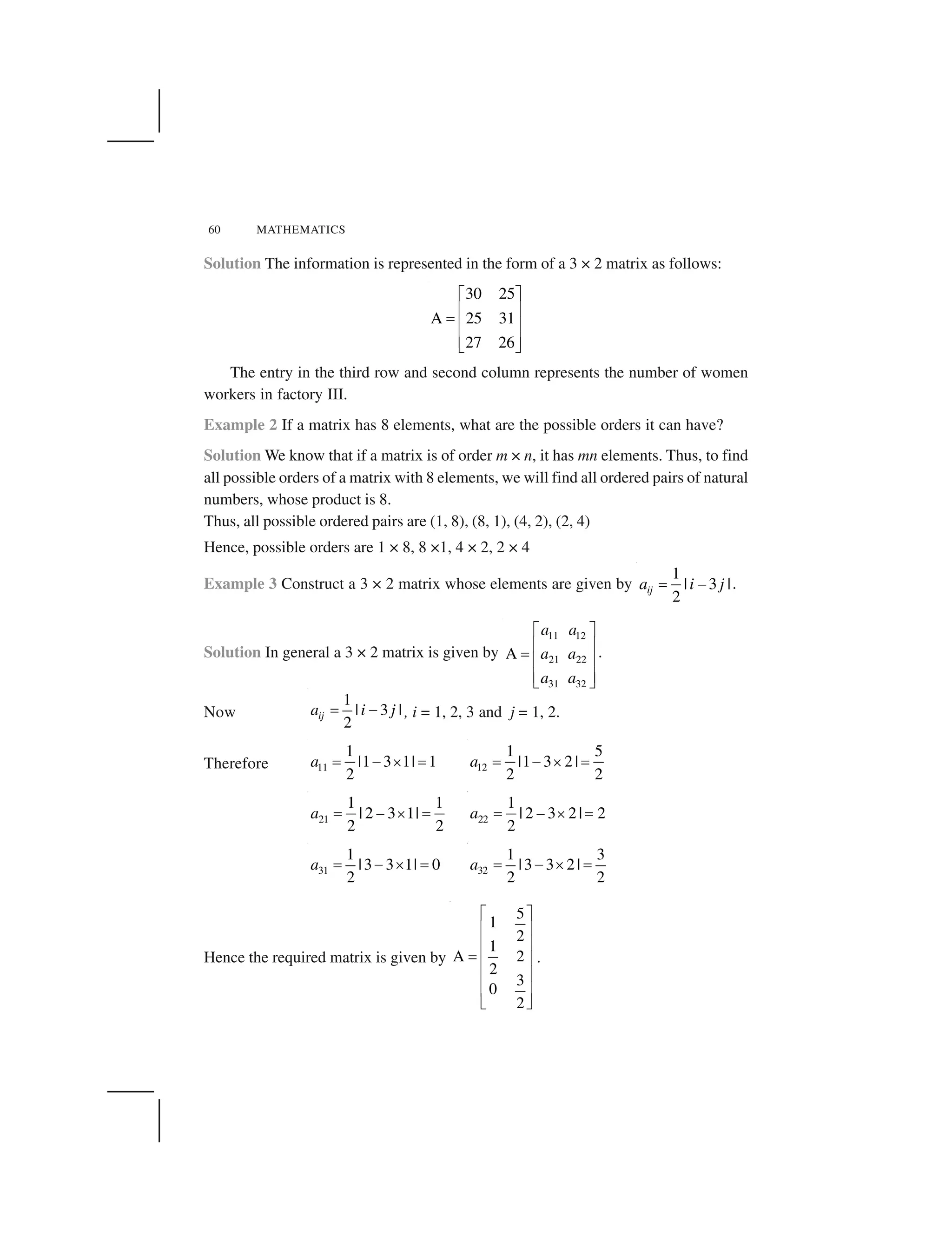
Example 1 Consider the following information regarding the number of men and women
workers in three factories I, II and III
Men workers Women workers
I 30 25
II 25 31
III 27 26
Represent the above information in the form of a 3 × 2 matrix. What does the entry
in the third row and second column represent?](https://image.slidesharecdn.com/ncert-class-12-mathematics-part-1-161112165946/75/Ncert-class-12-mathematics-part-1-62-2048.jpg)
![MATRICES 61
3.3 Types of Matrices
In this section, we shall discuss different types of matrices.
(i) Column matrix
A matrix is said to be a column matrix if it has only one column.
For example,
0
3
A 1
1/ 2
✁
✂ ✄
✂ ✄
✂ ✄☎ ✆
✂ ✄
✂ ✄✝ ✞
is a column matrix of order 4 × 1.
In general, A = [aij
] m × 1
is a column matrix of order m × 1.
(ii) Row matrix
A matrix is said to be a row matrix if it has only one row.
For example,
1 4
1
B 5 2 3
2 ✟
✠ ✡
☛ ☞
✌ ✍
✎ ✏
is a row matrix.
In general, B = [bij
] 1 × n
is a row matrix of order 1 × n.
(iii) Square matrix
A matrix in which the number of rows are equal to the number of columns, is
said to be a square matrix. Thus an m × n matrix is said to be a square matrix if
m = n and is known as a square matrix of order ‘n’.
For example
3 1 0
3
A 3 2 1
2
4 3 1
✑✒ ✓
✔ ✕
✔ ✕✖
✔ ✕
✔ ✕✑✗ ✘
is a square matrix of order 3.
In general, A = [aij
] m × m
is a square matrix of order m.
✙
Note If A = [aij
] is a square matrix of order n, then elements (entries) a11
, a22
, ..., ann
are said to constitute the diagonal, of the matrix A. Thus, if
1 3 1
A 2 4 1
3 5 6
✚✛ ✜
✢ ✣
✤ ✚
✢ ✣
✢ ✣✥ ✦
.
Then the elements of the diagonal of A are 1, 4, 6.](https://image.slidesharecdn.com/ncert-class-12-mathematics-part-1-161112165946/75/Ncert-class-12-mathematics-part-1-64-2048.jpg)
![62 MATHEMATICS
(iv) Diagonal matrix
A square matrix B = [bij
] m × m
is said to be a diagonal matrix if all its non
diagonal elements are zero, that is a matrix B = [bij
] m × m
is said to be a diagonal
matrix if bij
= 0, when i ☎ j.
For example, A = [4],
1 0
B
0 2
✁ ✂
✄ ✆ ✝
✞ ✟
,
1.1 0 0
C 0 2 0
0 0 3
✠✡ ☛
☞ ✌✍ ☞ ✌
☞ ✌✎ ✏
, are diagonal matrices
of order 1, 2, 3, respectively.
(v) Scalar matrix
A diagonal matrix is said to be a scalar matrix if its diagonal elements are equal,
that is, a square matrix B = [bij
] n × n
is said to be a scalar matrix if
bij
= 0, when i ☎ j
bij
= k, when i = j, for some constant k.
For example
A = [3],
1 0
B
0 1
✁ ✂
✄ ✆ ✝ ✞ ✟
,
3 0 0
C 0 3 0
0 0 3
✑ ✒
✓ ✔
✕ ✓ ✔
✓ ✔
✖ ✗
are scalar matrices of order 1, 2 and 3, respectively.
(vi) Identity matrix
A square matrix in which elements in the diagonal are all 1 and rest are all zero
is called an identity matrix. In other words, the square matrix A = [aij
] n × n
is an
identity matrix, if
1 if
0 if
ij
i j
a
i j
✄✘
✄ ✙
✚✛
.
We denote the identity matrix of order n by In
. When order is clear from the
context, we simply write it as I.
For example [1],
1 0
0 1
✁ ✂
✆ ✝
✞ ✟
,
1 0 0
0 1 0
0 0 1
✜ ✢
✣ ✤
✣ ✤
✣ ✤✥ ✦
are identity matrices of order 1, 2 and 3,
respectively.
Observe that a scalar matrix is an identity matrix when k = 1. But every identity
matrix is clearly a scalar matrix.](https://image.slidesharecdn.com/ncert-class-12-mathematics-part-1-161112165946/75/Ncert-class-12-mathematics-part-1-65-2048.jpg)
![MATRICES 63
(vii) Zero matrix
A matrix is said to be zero matrix or null matrix if all its elements are zero.
For example, [0],
0 0
0 0
✁
✂ ✄
☎ ✆
,
0 0 0
0 0 0
✁
✂ ✄
☎ ✆
, [0, 0] are all zero matrices. We denote
zero matrix by O. Its order will be clear from the context.
3.3.1 Equality of matrices
Definition 2 Two matrices A = [aij
] and B = [bij
] are said to be equal if
(i) they are of the same order
(ii) each element of A is equal to the corresponding element of B, that is aij
= bij
for
all i and j.
For example,
2 3 2 3
and
0 1 0 1
✁ ✁
✂ ✄ ✂ ✄
☎ ✆ ☎ ✆
are equal matrices but
3 2 2 3
and
0 1 0 1
✁ ✁
✂ ✄ ✂ ✄
☎ ✆ ☎ ✆
are
not equal matrices. Symbolically, if two matrices A and B are equal, we write A = B.
If
1.5 0
2 6
3 2
x y
z a
b c
✝✞ ✟✞ ✟
✠ ✡✠ ✡
☛
✠ ✡✠ ✡
✠ ✡✠ ✡☞ ✌ ☞ ✌
, then x = – 1.5, y = 0, z = 2, a = 6 , b = 3, c = 2
Example 4 If
3 4 2 7 0 6 3 2
6 1 0 6 3 2 2
3 21 0 2 4 21 0
x z y y
a c
b b
✍ ✍ ✎ ✎✏ ✑ ✏ ✑
✒ ✓ ✒ ✓
✎ ✎ ✔ ✎ ✎ ✍
✒ ✓ ✒ ✓
✒ ✓ ✒ ✓✎ ✎ ✍ ✎✕ ✖ ✕ ✖
Find the values of a, b, c, x, y and z.
Solution As the given matrices are equal, therefore, their corresponding elements
must be equal. Comparing the corresponding elements, we get
x + 3 = 0, z + 4 = 6, 2y – 7 = 3y – 2
a – 1 = – 3, 0 = 2c + 2 b – 3 = 2b + 4,
Simplifying, we get
a = – 2, b = – 7, c = – 1, x = – 3, y = –5, z = 2
Example 5 Find the values of a, b, c, and d from the following equation:
2 2 4 3
5 4 3 11 24
a b a b
c d c d
✗ ✘ ✘ ✁ ✁
✙✂ ✄ ✂ ✄
✘ ✗☎ ✆ ☎ ✆](https://image.slidesharecdn.com/ncert-class-12-mathematics-part-1-161112165946/75/Ncert-class-12-mathematics-part-1-66-2048.jpg)
![64 MATHEMATICS
Solution By equality of two matrices, equating the corresponding elements, we get
2a + b = 4 5c – d = 11
a – 2b = – 3 4c + 3d = 24
Solving these equations, we get
a = 1, b = 2, c = 3 and d = 4
EXERCISE 3.1
1. In the matrix
2 5 19 7
5
A 35 2 12
2
173 1 5
✁✂
✄ ☎
✄ ☎✆ ✂
✄ ☎
✄ ☎
✂✝ ✞
, write:
(i) The order of the matrix, (ii) The number of elements,
(iii) Write the elements a13
, a21
, a33
, a24
, a23
.
2. If a matrix has 24 elements, what are the possible orders it can have? What, if it
has 13 elements?
3. If a matrix has 18 elements, what are the possible orders it can have? What, if it
has 5 elements?
4. Construct a 2 × 2 matrix, A = [aij
], whose elements are given by:
(i)
2
( )
2
ij
i j
a
✟
✠ (ii) ij
i
a
j
✡ (iii)
2
( 2 )
2
ij
i j
a
✟
✠
5. Construct a 3 × 4 matrix, whose elements are given by:
(i)
1
| 3 |
2
ija i j☛ ☞ ✌ (ii) 2ija i j✆ ✂
6. Find the values of x, y and z from the following equations:
(i)
4 3
5 1 5
y z
x
✍ ✎ ✍ ✎
✏✑ ✒ ✑ ✒
✓ ✔ ✓ ✔
(ii)
2 6 2
5 5 8
x y
z xy
✕✍ ✎ ✍ ✎
✏✑ ✒ ✑ ✒
✕✓ ✔ ✓ ✔
(iii)
9
5
7
x y z
x z
y z
✖ ✖✗ ✘ ✗ ✘
✙ ✚ ✙ ✚
✖ ✛
✙ ✚ ✙ ✚
✙ ✚ ✙ ✚✖✜ ✢ ✜ ✢
7. Find the value of a, b, c and d from the equation:
2 1 5
2 3 0 13
a b a c
a b c d
✣ ✤ ✣✥ ✦ ✥ ✦
✧★ ✩ ★ ✩
✣ ✤✪ ✫ ✪ ✫](https://image.slidesharecdn.com/ncert-class-12-mathematics-part-1-161112165946/75/Ncert-class-12-mathematics-part-1-67-2048.jpg)
![MATRICES 65
8. A = [aij
]m × n
is a square matrix, if
(A) m < n (B) m > n (C) m = n (D) None of these
9. Which of the given values of x and y make the following pair of matrices equal
3 7 5
1 2 3
x
y x
✁ ✂
✄ ☎ ✆✝ ✞
,
0 2
8 4
y ✆✁ ✂
✄ ☎
✝ ✞
(A)
1
, 7
3
x y
✟
✠ ✠ (B) Not possible to find
(C) y = 7,
2
3
x
✡
☛ (D)
1 2
,
3 3
x y
✡ ✡
☛ ☛
10. The number of all possible matrices of order 3 × 3 with each entry 0 or 1 is:
(A) 27 (B) 18 (C) 81 (D) 512
3.4 Operations on Matrices
In this section, we shall introduce certain operations on matrices, namely, addition of
matrices, multiplication of a matrix by a scalar, difference and multiplication of matrices.
3.4.1 Addition of matrices
Suppose Fatima has two factories at places A and B. Each factory produces sport
shoes for boys and girls in three different price categories labelled 1, 2 and 3. The
quantities produced by each factory are represented as matrices given below:
Suppose Fatima wants to know the total production of sport shoes in each price
category. Then the total production
In category 1 : for boys (80 + 90), for girls (60 + 50)
In category 2 : for boys (75 + 70), for girls (65 + 55)
In category 3 : for boys (90 + 75), for girls (85 + 75)
This can be represented in the matrix form as
80 90 60 50
75 70 65 55
90 75 85 75
☞ ☞✌ ✍
✎ ✏☞ ☞✎ ✏
✎ ✏☞ ☞✑ ✒
.](https://image.slidesharecdn.com/ncert-class-12-mathematics-part-1-161112165946/75/Ncert-class-12-mathematics-part-1-68-2048.jpg)
![66 MATHEMATICS
This new matrix is the sum of the above two matrices. We observe that the sum of
two matrices is a matrix obtained by adding the corresponding elements of the given
matrices. Furthermore, the two matrices have to be of the same order.
Thus, if
11 12 13
21 22 23
A
a a a
a a a
✁
✂ ✄ ☎
✆ ✝
is a 2 × 3 matrix and
11 12 13
21 22 23
B
b b b
b b b
✁
✂ ✄ ☎
✆ ✝
is another
2×3 matrix. Then, we define
11 11 12 12 13 13
21 21 22 22 23 23
A + B
a b a b a b
a b a b a b
✞ ✞ ✞ ✁
✂ ✄ ☎
✞ ✞ ✞✆ ✝
.
In general, if A = [aij
] and B = [bij
] are two matrices of the same order, say m × n.
Then, the sum of the two matrices A and B is defined as a matrix C = [cij
]m × n
, where
cij
= aij
+ bij
, for all possible values of i and j.
Example 6 Given
3 1 1
A
2 3 0
✟ ✠✡
☛ ☞ ✌
✍ ✎
and
2 5 1
B 1
2 3
2
✏ ✑
✒ ✓
✔
✒ ✓✕
✒ ✓✖ ✗
, find A + B
Since A, B are of the same order 2 × 3. Therefore, addition of A and B is defined
and is given by
2 3 1 5 1 1 2 3 1 5 0
A+B 1 1
2 2 3 3 0 0 6
2 2
✏ ✑ ✏ ✑✘ ✘ ✕ ✘ ✘
✒ ✓ ✒ ✓
✔ ✔
✒ ✓ ✒ ✓✕ ✘ ✘
✒ ✓ ✒ ✓✖ ✗ ✖ ✗
✙
Note
1. We emphasise that if A and B are not of the same order, then A + B is not
defined. For example if
2 3
A
1 0
✚ ✛
✜ ✢ ✣
✤ ✥
,
1 2 3
B ,
1 0 1
✦ ✧
★ ✩ ✪
✫ ✬
then A + B is not defined.
2. We may observe that addition of matrices is an example of binary operation
on the set of matrices of the same order.
3.4.2 Multiplication of a matrix by a scalar
Now suppose that Fatima has doubled the production at a factory A in all categories
(refer to 3.4.1).](https://image.slidesharecdn.com/ncert-class-12-mathematics-part-1-161112165946/75/Ncert-class-12-mathematics-part-1-69-2048.jpg)
![MATRICES 67
Previously quantities (in standard units) produced by factory A were
Revised quantities produced by factory A are as given below:
Boys Girls
2 80 2 601
2 2 75 2 65
3 2 90 2 85
✁ ✂
✄ ☎ ✄ ☎
✄ ☎ ✆ ✝
This can be represented in the matrix form as
160 120
150 130
180 170
✞ ✟
✠ ✡
✠ ✡
✠ ✡☛ ☞
. We observe that
the new matrix is obtained by multiplying each element of the previous matrix by 2.
In general, we may define multiplication of a matrix by a scalar as follows: if
A = [aij
] m × n
is a matrix and k is a scalar, then kA is another matrix which is obtained
by multiplying each element of A by the scalar k.
In other words, kA = k[aij
]m × n
= [k (aij
)] m × n
, that is, (i, j)th
element of kA is kaij
for all possible values of i and j.
For example, if A =
3 1 1.5
5 7 3
2 0 5
✌ ✍
✎ ✏
✑✎ ✏
✎ ✏✒ ✓
, then
3A =
3 1 1.5 9 3 4.5
3 5 7 3 3 5 21 9
2 0 5 6 0 15
✌ ✍ ✌ ✍
✎ ✏ ✎ ✏
✑ ✔ ✑✎ ✏ ✎ ✏
✎ ✏ ✎ ✏
✒ ✓ ✒ ✓
Negative of a matrix The negative of a matrix is denoted by – A. We define
–A = (– 1) A.](https://image.slidesharecdn.com/ncert-class-12-mathematics-part-1-161112165946/75/Ncert-class-12-mathematics-part-1-70-2048.jpg)
![68 MATHEMATICS
For example, let A =
3 1
5 x
✁
✂ ✄
☎✆ ✝
, then – A is given by
– A = (– 1)
3 1 3 1
A ( 1)
5 5x x
✞ ✞✟ ✠ ✟ ✠
✡ ✞ ✡☛ ☞ ☛ ☞
✞ ✞✌ ✍ ✌ ✍
Difference of matrices If A = [aij
], B = [bij
] are two matrices of the same order,
say m × n, then difference A – B is defined as a matrix D = [dij
], where dij
= aij
– bij
,
for all value of i and j. In other words, D = A– B =A + (–1) B, that is sum of the matrix
A and the matrix – B.
Example 7 If
1 2 3 3 1 3
A and B
2 3 1 1 0 2
✞✟ ✠ ✟ ✠
✡ ✡☛ ☞ ☛ ☞
✞✌ ✍ ✌ ✍
, then find 2A – B.
Solution We have
2A – B =
1 2 3 3 1 3
2
2 3 1 1 0 2
☎ ✁ ✁
☎✂ ✄ ✂ ✄
☎✆ ✝ ✆ ✝
=
2 4 6 3 1 3
4 6 2 1 0 2
☎ ☎ ✁ ✁
✎✂ ✄ ✂ ✄
☎✆ ✝ ✆ ✝
=
2 3 4 1 6 3 1 5 3
4 1 6 0 2 2 5 6 0
☎ ✎ ☎ ☎ ✁ ✁
✏✂ ✄ ✂ ✄
✎ ✎ ☎✆ ✝ ✆ ✝
3.4.3 Properties of matrix addition
The addition of matrices satisfy the following properties:
(i) Commutative Law If A = [aij
], B = [bij
] are matrices of the same order, say
m × n, then A + B = B + A.
Now A + B = [aij
] + [bij
] = [aij
+ bij
]
= [bij
+ aij
] (addition of numbers is commutative)
= ([bij
] + [aij
]) = B + A
(ii) Associative Law For any three matrices A = [aij
], B = [bij
], C = [cij
] of the
same order, say m × n, (A + B) + C = A + (B + C).
Now (A + B) + C = ([aij
] + [bij
]) + [cij
]
= [aij
+ bij
] + [cij
] = [(aij
+ bij
) + cij
]
= [aij
+ (bij
+ cij
)] (Why?)
= [aij
] + [(bij
+ cij
)] = [aij
] + ([bij
] + [cij
]) = A + (B + C)](https://image.slidesharecdn.com/ncert-class-12-mathematics-part-1-161112165946/75/Ncert-class-12-mathematics-part-1-71-2048.jpg)
![MATRICES 69
(iii) Existence of additive identity Let A = [aij
] be an m × n matrix and
O be an m × n zero matrix, then A + O = O + A = A. In other words, O is the
additive identity for matrix addition.
(iv) The existence of additive inverse Let A = [aij
]m × n
be any matrix, then we
have another matrix as – A = [– aij
]m × n
such that A + (– A) = (– A) + A= O. So
– A is the additive inverse of A or negative of A.
3.4.4 Properties of scalar multiplication of a matrix
If A = [aij
] and B = [bij
] be two matrices of the same order, say m × n, and k and l are
scalars, then
(i) k(A +B) = k A + kB, (ii) (k + l)A = k A + l A
(ii) k (A + B) = k ([aij
] + [bij
])
= k [aij
+ bij
] = [k (aij
+ bij
)] = [(k aij
) + (k bij
)]
= [k aij
] + [k bij
] = k [aij
] + k [bij
] = kA + kB
(iii) ( k + l) A = (k + l) [aij
]
= [(k + l) aij
] + [k aij
] + [l aij
] = k [aij
] + l [aij
] = k A + l A
Example 8 If
8 0 2 2
A 4 2 and B 4 2
3 6 5 1
✁ ✂ ✁ ✂
✄ ☎ ✄ ☎✆ ✆✄ ☎ ✄ ☎
✄ ☎ ✄ ☎ ✝ ✞ ✝ ✞
, then find the matrix X, such that
2A + 3X = 5B.
Solution We have 2A + 3X = 5B
or 2A + 3X – 2A = 5B – 2A
or 2A – 2A + 3X = 5B – 2A (Matrix addition is commutative)
or O + 3X = 5B – 2A (– 2A is the additive inverse of 2A)
or 3X = 5B – 2A (O is the additive identity)
or X =
1
3
(5B – 2A)
or
2 2 8 0
1
X 5 4 2 2 4 2
3
5 1 3 6
✟ ✠✡☛ ☞ ☛ ☞
✌ ✍✎ ✏ ✎ ✏✑ ✡ ✡✌ ✍✎ ✏ ✎ ✏
✌ ✍✎ ✏ ✎ ✏✡✒ ✓ ✒ ✓✔ ✕
=
10 10 16 0
1
20 10 8 4
3
25 5 6 12
✟ ✠✡ ✡☛ ☞ ☛ ☞
✌ ✍✎ ✏ ✎ ✏✖ ✡✌ ✍✎ ✏ ✎ ✏
✌ ✍✎ ✏ ✎ ✏✡ ✡ ✡✒ ✓ ✒ ✓✔ ✕](https://image.slidesharecdn.com/ncert-class-12-mathematics-part-1-161112165946/75/Ncert-class-12-mathematics-part-1-72-2048.jpg)
![MATRICES 73
Again, the above information can be represented as follows:
Requirements Prices per piece (in Rupees) Money needed (in Rupees)
2 5
8 10
✁
✂ ✄
☎ ✆
4
40
✁
✂ ✄
☎ ✆
4 2 40 5 208
8 4 10 4 0 432
✝ ✞ ✝ ✁ ✁
✟✂ ✄ ✂ ✄
✝ ✞ ✝☎ ✆ ☎ ✆
Now, the information in both the cases can be combined and expressed in terms of
matrices as follows:
Requirements Prices per piece (in Rupees) Money needed (in Rupees)
2 5
8 10
✁
✂ ✄
☎ ✆
5 4
50 40
✁
✂ ✄
☎ ✆
5 2 5 50 4 2 40 5
8 5 10 5 0 8 4 10 4 0
✝ ✞ ✝ ✝ ✞ ✝ ✁
✂ ✄
✝ ✞ ✝ ✝ ✞ ✝☎ ✆
=
260 208
540 432
✠ ✡
☛ ☞
✌ ✍
The above is an example of multiplication of matrices. We observe that, for
multiplication of two matricesAand B, the number of columns inAshould be equal to
the number of rows in B. Furthermore for getting the elements of the product matrix,
we take rows of A and columns of B, multiply them element-wise and take the sum.
Formally, we define multiplication of matrices as follows:
The product of two matrices A and B is defined if the number of columns of A is
equal to the number of rows of B. Let A = [aij
] be an m × n matrix and B = [bjk
] be an
n × p matrix. Then the product of the matrices A and B is the matrix C of order m × p.
To get the (i, k)th
element cik
of the matrix C, we take the ith
row of A and kth
column
of B, multiply them elementwise and take the sum of all these products. In other words,
if A = [aij
]m × n
, B = [bjk
]n × p
, then the ith
row of A is [ai1
ai2
... ain
] and the kth
column of
B is
1
2
k
k
nk
b
b
b
✎ ✏
✑ ✒
✑ ✒
✑ ✒
✑ ✒
✑ ✒
✓ ✔
, then cik
= ai1
b1k
+ ai2
b2k
+ ai3
b3k
+ ... + ain
bnk
=
1
n
ij jk
j
a b
✕
✖ .
The matrix C = [cik
]m × p
is the product of A and B.
For example, if
1 1 2
C
0 3 4
✗ ✁
✟ ✂ ✄
☎ ✆
and
2 7
1D 1
5 4
✘ ✙
✚ ✛
✜ ✢
✚ ✛
✚ ✛✢✣ ✤
, then the product CD is defined](https://image.slidesharecdn.com/ncert-class-12-mathematics-part-1-161112165946/75/Ncert-class-12-mathematics-part-1-76-2048.jpg)

![80 MATHEMATICS
Solution We have
BA =
40,000 50,000 250,000 X
Y120,000 +100,000 +500,000
✁✂ ✄
☎ ✆ ✁✝ ✞
=
340,000 X
Y720,000
✁✂ ✄
☎ ✆ ✁✝ ✞
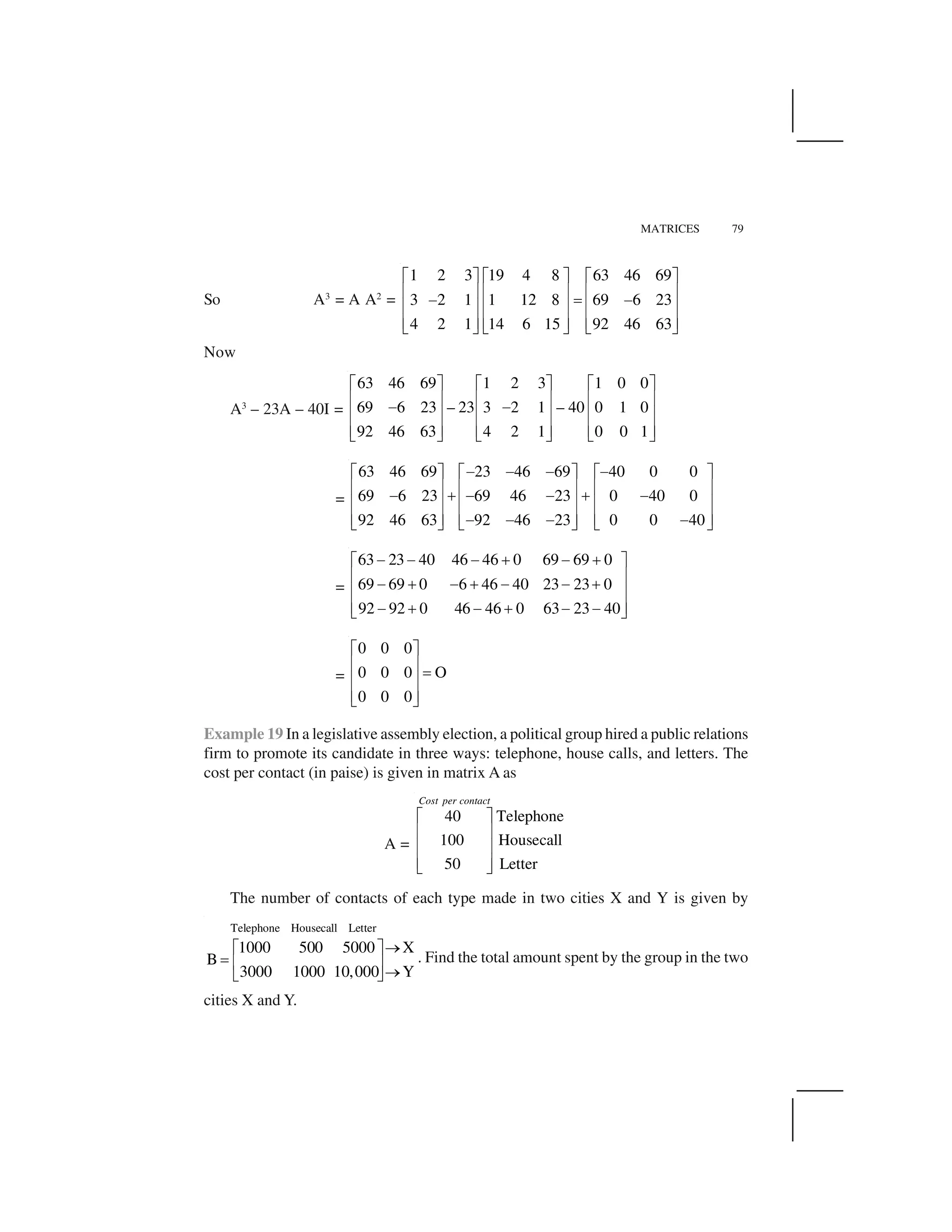
So the total amount spent by the group in the two cities is 340,000 paise and
720,000 paise, i.e., Rs 3400 and Rs 7200, respectively.
EXERCISE 3.2
1. Let
2 4 1 3 2 5
A , B , C
3 2 2 5 3 4
✟✂ ✄ ✂ ✄ ✂ ✄
✠ ✠ ✠☎ ✆ ☎ ✆ ☎ ✆✟✝ ✞ ✝ ✞ ✝ ✞
Find each of the following:
(i) A + B (ii) A – B (iii) 3A – C
(iv) AB (v) BA
2. Compute the following:
(i)
a b a b
b a b a
✂ ✄ ✂ ✄
☎ ✆ ☎ ✆✟✝ ✞ ✝ ✞
(ii)
2 2 2 2
2 2 2 2
2 2
2 2
a b b c ab bc
ac aba c a b
✡ ☛☞ ☞ ✡ ☛
☞✌ ✍ ✌ ✍✎ ✎☞ ☞ ✏ ✑✌ ✍✏ ✑
(iii)
1 4 6 12 7 6
8 5 16 8 0 5
2 8 5 3 2 4
✒ ✒✓ ✔ ✓ ✔
✕ ✖ ✕ ✖✗✕ ✖ ✕ ✖
✕ ✖ ✕ ✖✘ ✙ ✘ ✙
(iv)
2 2 2 2
2 2 2 2
cos sin sin cos
sin cos cos sin
x x x x
x x x x
✚ ✛ ✚ ✛
✜✢ ✣ ✢ ✣
✢ ✣ ✢ ✣✤ ✥ ✤ ✥
3. Compute the indicated products.
(i)
a b a b
b a b a
✟✂ ✄ ✂ ✄
☎ ✆ ☎ ✆✟✝ ✞ ✝ ✞
(ii)
1
2
3
✦ ✧
★ ✩
★ ✩
★ ✩✪ ✫
[2 3 4] (iii)
1 2 1 2 3
2 3 2 3 1
✟✂ ✄ ✂ ✄
☎ ✆ ☎ ✆
✝ ✞ ✝ ✞
(iv)
2 3 4 1 3 5
3 4 5 0 2 4
4 5 6 3 0 5
✬✦ ✧ ✦ ✧
★ ✩ ★ ✩
★ ✩ ★ ✩
★ ✩ ★ ✩✪ ✫ ✪ ✫
(v)
2 1
1 0 1
3 2
1 2 1
1 1
✦ ✧
✦ ✧★ ✩
★ ✩★ ✩ ✬✪ ✫★ ✩✬✪ ✫
(vi)
2 3
3 1 3
1 0
1 0 2
3 1
✒✓ ✔
✒✓ ✔ ✕ ✖
✕ ✖ ✕ ✖✒✘ ✙ ✕ ✖✘ ✙](https://image.slidesharecdn.com/ncert-class-12-mathematics-part-1-161112165946/75/Ncert-class-12-mathematics-part-1-83-2048.jpg)
![MATRICES 83
20. The bookshop of a particular school has 10 dozen chemistry books, 8 dozen
physics books, 10 dozen economics books. Their selling prices are Rs 80, Rs 60
and Rs 40 each respectively. Find the total amount the bookshop will receive
from selling all the books using matrix algebra.
Assume X, Y, Z, W and P are matrices of order 2 × n, 3 × k, 2 × p, n × 3 and p × k,
respectively. Choose the correct answer in Exercises 21 and 22.
21. The restriction on n, k and p so that PY + WY will be defined are:
(A) k = 3, p = n (B) k is arbitrary, p = 2
(C) p is arbitrary, k = 3 (D) k = 2, p = 3
22. If n = p, then the order of the matrix 7X – 5Z is:
(A) p × 2 (B) 2 × n (C) n × 3 (D) p × n
3.5. Transpose of a Matrix
In this section, we shall learn about transpose of a matrix and special types of matrices
such as symmetric and skew symmetric matrices.
Definition 3 IfA = [aij
] be an m × n matrix, then the matrix obtained by interchanging
the rows and columns of A is called the transpose of A. Transpose of the matrix A is
denoted by A✝ or (AT
). In other words, if A = [aij
]m × n
, then A✝ = [aji
]n × m
. For example,
if
2 3
3 2
3 5 3 3 0
A 3 1 , then A 1
5 1
0 1 5
5
✁ ✂ ✁ ✂
✄ ☎ ✄ ☎
✆ ✞ ✆✄ ☎ ✟✄ ☎
✄ ☎ ✄ ☎✟ ✠ ✡
✄ ☎
✠ ✡
3.5.1 Properties of transpose of the matrices
We now state the following properties of transpose of matrices without proof. These
may be verified by taking suitable examples.
For any matrices A and B of suitable orders, we have
(i) (A✝)✝ = A, (ii) (kA)✝ = kA✝ (where k is any constant)
(iii) (A + B)✝ = A✝ + B✝ (iv) (A B)✝ = B✝ A✝
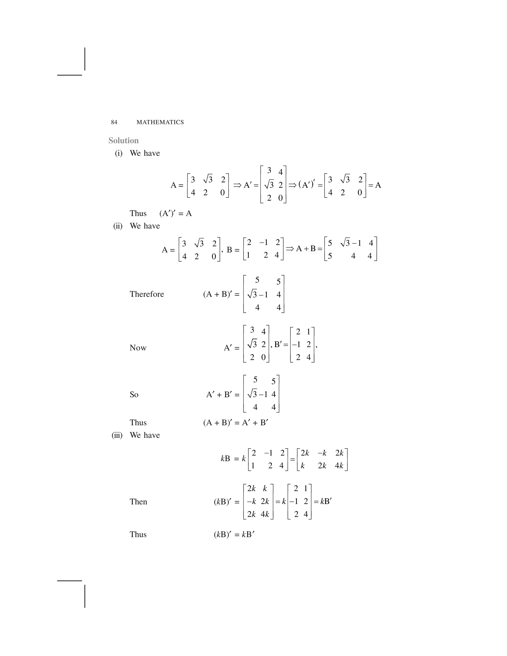
Example 20 If
2 1 23 3 2
A and B
1 2 44 2 0
☛ ☞ ✌☛ ☞
✍ ✍✎ ✏ ✎ ✏
✑ ✒✑ ✒
, verify that
(i) (A✝)✝ = A, (ii) (A + B)✝ = A✝ + B✝,
(iii) (kB)✝ = kB✝, where k is any constant.](https://image.slidesharecdn.com/ncert-class-12-mathematics-part-1-161112165946/75/Ncert-class-12-mathematics-part-1-86-2048.jpg)
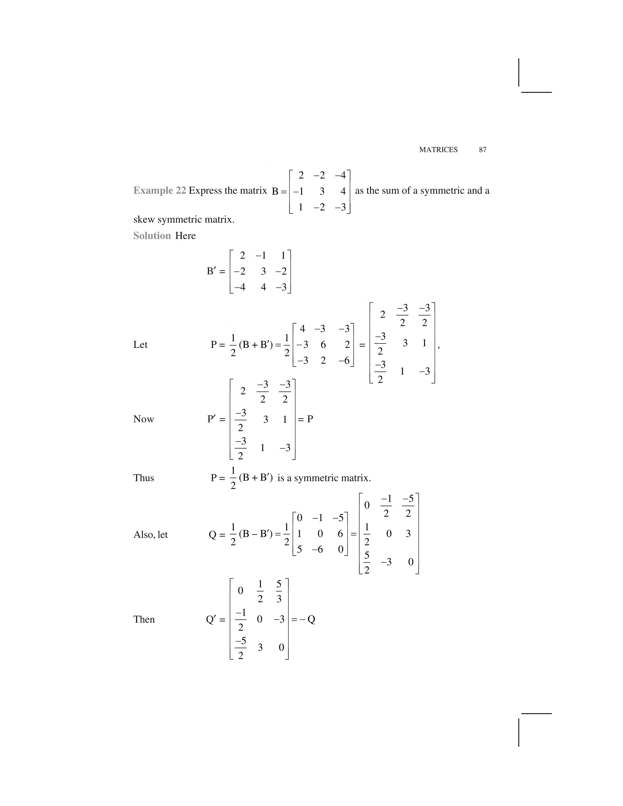
![MATRICES 85
Example 21 If ✁
2
A 4 , B 1 3 6
5
✂✄ ☎
✆ ✝
✞ ✞ ✂
✆ ✝
✆ ✝✟ ✠
, verify that (AB)✡ = B✡A✡.
Solution We have
A = ☛ ☞
2
4 , B 1 3 6
5
✌✍ ✎
✏ ✑
✒ ✌
✏ ✑
✏ ✑✓ ✔
then AB = ✕ ✖
2
4 1 3 6
5
✌✍ ✎
✏ ✑
✌
✏ ✑
✏ ✑✓ ✔
=
2 6 12
4 12 24
5 15 30
✌ ✌✍ ✎
✏ ✑
✌
✏ ✑
✏ ✑✌✓ ✔
Now A✡ = [–2 4 5] ,
1
B 3
6
✍ ✎
✏ ✑
✗ ✒
✏ ✑
✏ ✑✌✓ ✔
B✡A✡ = ✘ ✙
1 2 4 5
3 2 4 5 6 12 15 (AB)
6 12 24 30
✂✄ ☎ ✄ ☎
✆ ✝ ✆ ✝
✚✂ ✞ ✂ ✞
✆ ✝ ✆ ✝
✆ ✝ ✆ ✝✂ ✂ ✂✟ ✠ ✟ ✠
Clearly (AB)✡ = B✡A✡
3.6 Symmetric and Skew Symmetric Matrices
Definition 4 A square matrix A = [aij
] is said to be symmetric if A✡ = A, that is,
[aij
] = [aji
] for all possible values of i and j.
For example
3 2 3
A 2 1.5 1
3 1 1
✛ ✜
✢ ✣
✤ ✥ ✥✢ ✣
✢ ✣✥✦ ✧
is a symmetric matrix as A✡ = A
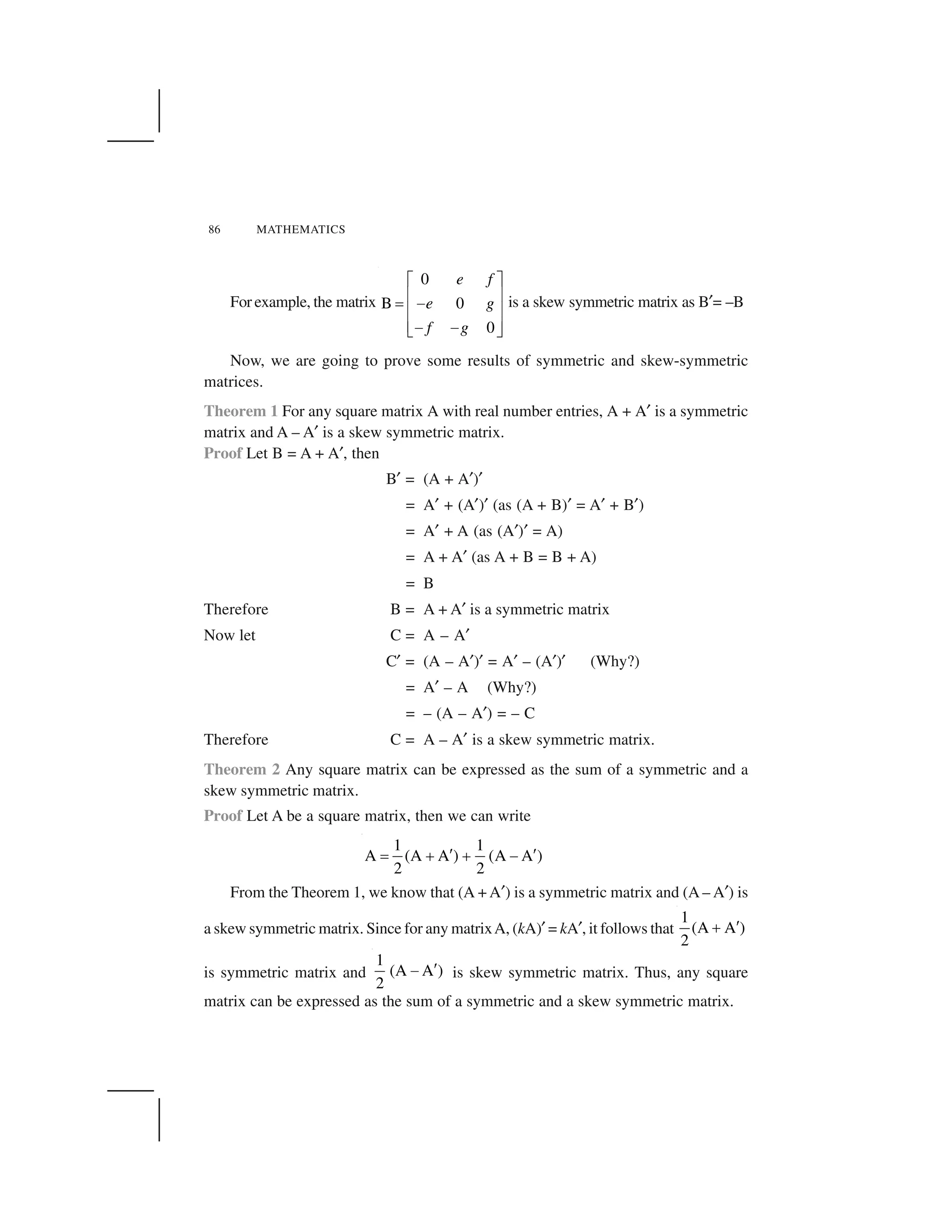
Definition 5 A square matrix A = [aij
] is said to be skew symmetric matrix if
A✡ = – A, that is aji
= – aij
for all possible values of i and j. Now, if we put i = j, we
have aii
= – aii
. Therefore 2aii
= 0 or aii
= 0 for all i’s.
This means that all the diagonal elements of a skew symmetric matrix are zero.](https://image.slidesharecdn.com/ncert-class-12-mathematics-part-1-161112165946/75/Ncert-class-12-mathematics-part-1-88-2048.jpg)
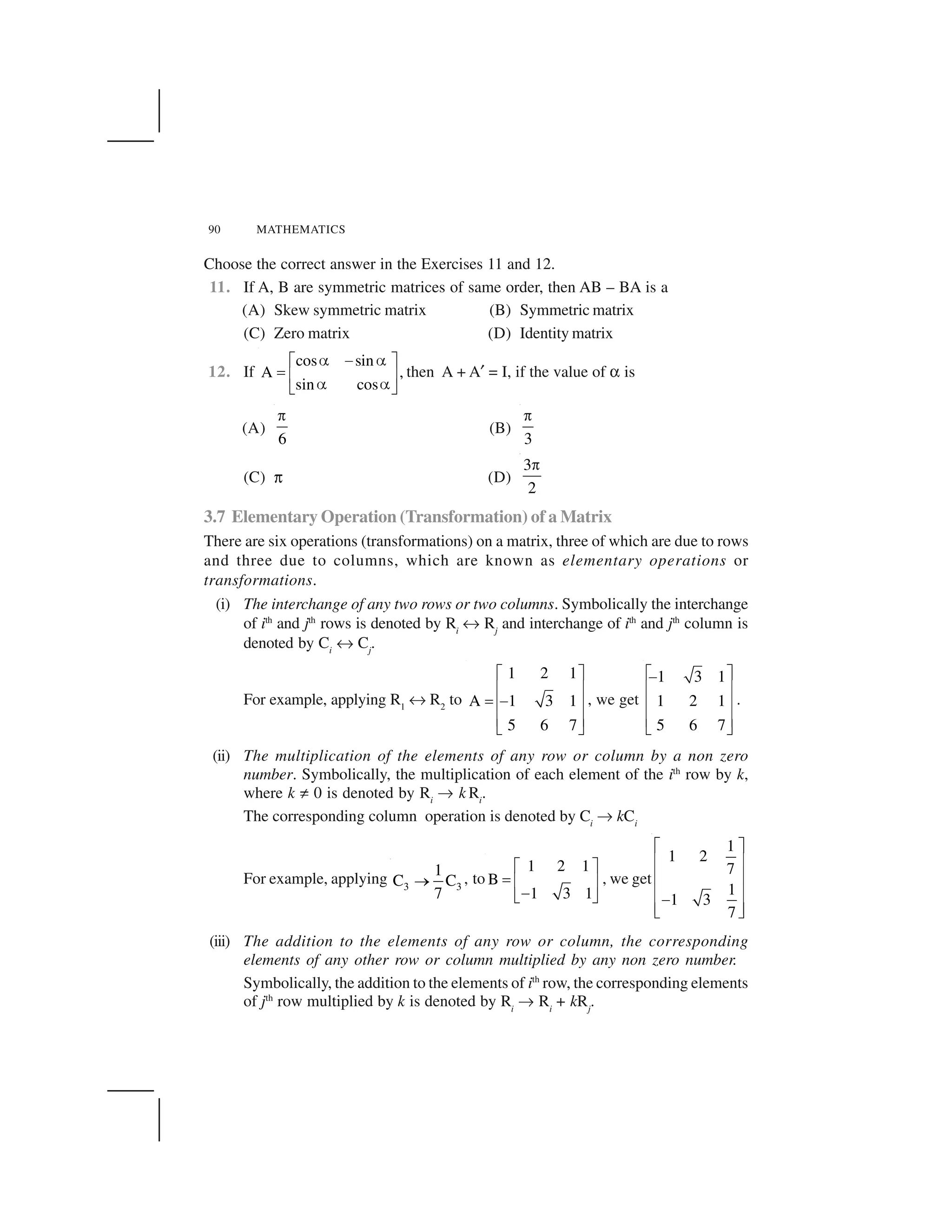
![MATRICES 91
The corresponding column operation is denoted by Ci
✡ Ci
+ kCj
.
For example, applying R2
✡ R2
– 2R1
, to
1 2
C
2 1
✁
✂ ✄ ☎
✆✝ ✞
, we get
1 2
0 5
✁
✄ ☎
✆✝ ✞
.
3.8 Invertible Matrices
Definition 6 If A is a square matrix of order m, and if there exists another square
matrix B of the same order m, such that AB = BA = I, then B is called the inverse
matrix of A and it is denoted by A– 1
. In that case A is said to be invertible.
For example, let A =
2 3
1 2
✟ ✠
☛ ☞
✌ ✍
and B =
2 3
1 2
✎✟ ✠
☛ ☞
✎✌ ✍
be two matrices.
Now AB =
2 3 2 3
1 2 1 2
✎✟ ✠ ✟ ✠
☛ ☞ ☛ ☞
✎✌ ✍ ✌ ✍
=
4 3 6 6 1 0
I
2 2 3 4 0 1
✎ ✎ ✏✟ ✠ ✟ ✠
✑ ✑☛ ☞ ☛ ☞
✎ ✎ ✏✌ ✍ ✌ ✍
Also BA =
1 0
I
0 1
✟ ✠
✑☛ ☞
✌ ✍
. Thus B is the inverse of A, in other
words B = A– 1
and A is inverse of B, i.e., A = B–1
✒
Note
1. A rectangular matrix does not possess inverse matrix, since for products BA
and AB to be defined and to be equal, it is necessary that matrices A and B
should be square matrices of the same order.
2. If B is the inverse of A, then A is also the inverse of B.
Theorem 3 (Uniqueness of inverse) Inverse of a square matrix, if it exists, is unique.
Proof Let A = [aij
] be a square matrix of order m. If possible, let B and C be two
inverses of A. We shall show that B = C.
Since B is the inverse of A
AB = BA = I ... (1)
Since C is also the inverse of A
AC = CA = I ... (2)
Thus B = BI = B (AC) = (BA) C = IC = C
Theorem 4 If A and B are invertible matrices of the same order, then (AB)–1
= B–1
A–1
.](https://image.slidesharecdn.com/ncert-class-12-mathematics-part-1-161112165946/75/Ncert-class-12-mathematics-part-1-94-2048.jpg)
![MATRICES 101
10. A manufacturer produces three products x, y, z which he sells in two markets.
Annual sales are indicated below:
Market Products
I 10,000 2,000 18,000
II 6,000 20,000 8,000
(a) If unit sale prices of x, y and z are Rs 2.50, Rs 1.50 and Rs 1.00, respectively,
find the total revenue in each market with the help of matrix algebra.
(b) If the unit costs of the above three commodities are Rs 2.00, Rs 1.00 and 50
paise respectively. Find the gross profit.
11. Find the matrix X so that
1 2 3 7 8 9
X
4 5 6 2 4 6
✁ ✂ ✁ ✂
✄☎ ✆ ☎ ✆
✝ ✞ ✝ ✞
12. If A and B are square matrices of the same order such thatAB = BA, then prove
by induction that ABn
= Bn
A. Further, prove that (AB)n
= An
Bn
for all n ✟ N.
Choose the correct answer in the following questions:
13. If A =
✠ ✡
☛ ✠
✁ ✂
☎ ✆ ✝ ✞
is such that A² = I, then
(A) 1 + ☞² + ✌✍ = 0 (B) 1 – ☞² + ✌✍ = 0
(C) 1 – ☞² – ✌✍ = 0 (D) 1 + ☞² – ✌✍ = 0
14. If the matrix A is both symmetric and skew symmetric, then
(A) A is a diagonal matrix (B) A is a zero matrix
(C) A is a square matrix (D) None of these
15. If A is square matrix such that A2
= A, then (I + A)³ – 7 A is equal to
(A) A (B) I – A (C) I (D) 3A
Summary
✎ A matrix is an ordered rectangular array of numbers or functions.
✎ A matrix having m rows and n columns is called a matrix of order m × n.
✎ [aij
]m × 1
is a column matrix.
✎ [aij
]1 × n
is a row matrix.
✎ An m × n matrix is a square matrix if m = n.
✎ A = [aij
]m × m
is a diagonal matrix if aij
= 0, when i ✏ j.](https://image.slidesharecdn.com/ncert-class-12-mathematics-part-1-161112165946/75/Ncert-class-12-mathematics-part-1-104-2048.jpg)
![102 MATHEMATICS
A = [aij
]n × n
is a scalar matrix if aij
= 0, when i ☎ j, aij
= k, (k is some
constant), when i = j.
A = [aij
]n × n
is an identity matrix, if aij
= 1, when i = j, aij
= 0, when i ☎ j.
A zero matrix has all its elements as zero.
A = [aij
] = [bij
] = B if (i) A and B are of same order, (ii) aij
= bij
for all
possible values of i and j.
kA = k[aij
]m × n
= [k(aij
)]m × n
– A = (–1)A
A – B = A + (–1) B
A + B = B + A
(A + B) + C = A + (B + C), where A, B and C are of same order.
k(A + B) = kA + kB, where A and B are of same order, k is constant.
(k + l ) A = kA + lA, where k and l are constant.
If A = [aij
]m × n
and B = [bjk
]n × p
, then AB = C = [cik
]m × p
, where
1
n
ik ij jk
j
c a b
✁
✂✄
(i) A(BC) = (AB)C, (ii) A(B + C) = AB + AC, (iii) (A+ B)C = AC + BC
If A = [aij
]m × n
, then A✝ or AT
= [aji
]n × m
(i) (A✝)✝= A, (ii) (kA)✝= kA✝, (iii) (A + B)✝= A✝+ B✝, (iv) (AB)✝= B✝A✝
A is a symmetric matrix if A✝= A.
A is a skew symmetric matrix if A✝= –A.
Any square matrix can be represented as the sum of a symmetric and a
skew symmetric matrix.
Elementary operations of a matrix are as follows:
(i) Ri
✠ Rj
or Ci
✠ Cj
(ii) Ri
✡ kRi
or Ci
✡ kCi
(iii) Ri
✡ Ri
+ kRj
or Ci
✡ Ci
+ kCj
If A and B are two square matrices such that AB = BA = I, then B is the
inverse matrix of A and is denoted by A–1
and A is the inverse of B.
Inverse of a square matrix, if it exists, is unique.
—✆✆—](https://image.slidesharecdn.com/ncert-class-12-mathematics-part-1-161112165946/75/Ncert-class-12-mathematics-part-1-105-2048.jpg)
![All Mathematical truths are relative and conditional. — C.P. STEINMETZ
4.1 Introduction
In the previous chapter, we have studied about matrices
and algebra of matrices. We have also learnt that a system
of algebraic equations can be expressed in the form of
matrices. This means, a system of linear equations like
a1
x + b1
y = c1
a2
x + b2
y = c2
can be represented as 1 1 1
2 2 2
a b cx
a b cy
✁ ✂ ✁ ✂✁ ✂✄☎ ✆ ☎ ✆☎ ✆✝ ✞✝ ✞ ✝ ✞. Now, this
system of equations has a unique solution or not, is
determined by the number a1
b2
– a2
b1
. (Recall that if
1 1
2 2
a b
a b
✟ or, a1
b2
– a2
b1
✠ 0, then the system of linear
equations has a unique solution). The number a1
b2
– a2
b1
which determines uniqueness of solution is associated with the matrix 1 1
2 2
A
a b
a b
✁ ✂✄☎ ✆✝ ✞
and is called the determinant of A or det A. Determinants have wide applications in
Engineering, Science, Economics, Social Science, etc.
In this chapter, we shall study determinants up to order three only with real entries.
Also, we will study various properties of determinants, minors, cofactors and applications
of determinants in finding the area of a triangle, adjoint and inverse of a square matrix,
consistency and inconsistency of system of linear equations and solution of linear
equations in two or three variables using inverse of a matrix.
4.2 Determinant
To every square matrix A = [aij
] of order n, we can associate a number (real or
complex) called determinant of the square matrix A, where aij
= (i, j)th
element of A.
Chapter 4
DETERMINANTS
P.S. Laplace
(1749-1827)](https://image.slidesharecdn.com/ncert-class-12-mathematics-part-1-161112165946/75/Ncert-class-12-mathematics-part-1-106-2048.jpg)
![104 MATHEMATICS
This may be thought of as a function which associates each square matrix with a
unique number (real or complex). If M is the set of square matrices, K is the set of
numbers (real or complex) and f : M ✄ K is defined by f (A) = k, where A ☎ M and
k ☎ K, then f (A) is called the determinant of A. It is also denoted by |A| or det A or ✆.
If A =
a b
c d
✁
✂ ✝
✞ ✟
, then determinant of A is written as |A| =
a b
c d
= det (A)
Remarks
(i) For matrix A, |A| is read as determinant of A and not modulus of A.
(ii) Only square matrices have determinants.
4.2.1 Determinant of a matrix of order one
Let A = [a ] be the matrix of order 1, then determinant of A is defined to be equal to a
4.2.2 Determinant of a matrix of order two
Let A =
11 12
21 22
a a
a a
✁
✂ ✝
✞ ✟
be a matrix of order 2 × 2,
then the determinant of A is defined as:
det (A) = |A| = ✆ = = a11
a22
– a21
a12
Example 1 Evaluate
2 4
–1 2
.
Solution We have
2 4
–1 2
= 2(2) – 4(–1) = 4 + 4 = 8.
Example 2 Evaluate
1
– 1
x x
x x
✠
Solution We have
1
– 1
x x
x x
✡
= x (x) – (x + 1) (x – 1) = x2
– (x2
– 1) = x2
– x2
+ 1 = 1
4.2.3 Determinant of a matrix of order 3 × 3
Determinant of a matrix of order three can be determined by expressing it in terms of
second order determinants. This is known as expansion of a determinant along
a row (or a column). There are six ways of expanding a determinant of order](https://image.slidesharecdn.com/ncert-class-12-mathematics-part-1-161112165946/75/Ncert-class-12-mathematics-part-1-107-2048.jpg)
![DETERMINANTS 105
3 corresponding to each of three rows (R1
, R2
and R3
) and three columns (C1
, C2
and
C3
) giving the same value as shown below.
Consider the determinant of square matrix A = [aij
]3 × 3
i.e., | A | = 21 22 23
31 32 33
a a a
a a a
11 12 13a a a
Expansion along first Row (R1
)
Step 1 Multiply first element a11
of R1
by (–1)(1 + 1)
[(–1)sum of suffixes in a11] and with the
second order determinant obtained by deleting the elements of first row (R1
) and first
column (C1
) of | A | as a11
lies in R1
and C1
,
i.e., (–1)1 + 1
a11
22 23
32 33
a a
a a
Step 2 Multiply 2nd element a12
of R1
by (–1)1 + 2
[(–1)sum of suffixes in a12] and the second
order determinant obtained by deleting elements of first row (R1
) and 2nd column (C2
)
of | A | as a12
lies in R1
and C2
,
i.e., (–1)1 + 2
a12
21 23
31 33
a a
a a
Step 3 Multiply third element a13
of R1
by (–1)1 + 3
[(–1)sum of suffixes in a13] and the second
order determinant obtained by deleting elements of first row (R1
) and third column (C3
)
of | A | as a13
lies in R1
and C3
,
i.e., (–1)1 + 3
a13
21 22
31 32
a a
a a
Step 4 Now the expansion of determinant of A, that is, | A | written as sum of all three
terms obtained in steps 1, 2 and 3 above is given by
det A = |A| = (–1)1 + 1
a11
22 23 21 231 2
12
32 33 31 33
(–1)
a a a a
a
a a a a
✁
+
21 221 3
13
31 32
(–1)
a a
a
a a
or |A| = a11
(a22
a33
– a32
a23
) – a12
(a21
a33
– a31
a23
)
+ a13
(a21
a32
– a31
a22
)](https://image.slidesharecdn.com/ncert-class-12-mathematics-part-1-161112165946/75/Ncert-class-12-mathematics-part-1-108-2048.jpg)
![DETERMINANTS 111
Expanding along first row, we get
✆= a1
(b2
c3
– b3
c2
) – a2
(b1
c3
– b3
c1
) + a3
(b1
c2
– b2
c1
)
Interchanging first and third rows, the new determinant obtained is given by
✆1
=
1 2 3
1 2 3
1 2 3
c c c
b b b
a a a
Expanding along third row, we get
✆1
= a1
(c2
b3
– b2
c3
) – a2
(c1
b3
– c3
b1
) + a3
(b2
c1
– b1
c2
)
= – [a1
(b2
c3
– b3
c2
) – a2
(b1
c3
– b3
c1
) + a3
(b1
c2
– b2
c1
)]
Clearly ✆1
= – ✆Similarly, we can verify the result by interchanging any two columns.
Note We can denote the interchange of rows by Ri
✠Rj
and interchange of
columns by Ci
✠Cj
.
Example 7 Verify Property 2 for ✆=
2 –3 5
6 0 4
1 5 –7
.
Solution ✆=
2 –3 5
6 0 4
1 5 –7
= – 28 (See Example 6)
Interchanging rows R2
and R3
i.e., R2
✠R3
, we have
✆1
=
2 –3 5
1 5 –7
6 0 4
Expanding the determinant ✆1
along first row, we have
✆1
=
5 –7 1 –7 1 5
2 – (–3) 5
0 4 6 4 6 0
✁
= 2 (20 – 0) + 3 (4 + 42) + 5 (0 – 30)
= 40 + 138 – 150 = 28](https://image.slidesharecdn.com/ncert-class-12-mathematics-part-1-161112165946/75/Ncert-class-12-mathematics-part-1-114-2048.jpg)
![112 MATHEMATICS
Clearly ✆1
= – ✆
Hence, Property 2 is verified.
Property 3 If any two rows (or columns) of a determinant are identical (all corresponding
elements are same), then value of determinant is zero.
Proof If we interchange the identical rows (or columns) of the determinant ✆, then ✆
does not change. However, by Property 2, it follows that ✆ has changed its sign
Therefore ✆ = – ✆
or ✆ = 0
Let us verify the above property by an example.
Example 8 Evaluate ✆ =
3 2 3
2 2 3
3 2 3
Solution Expanding along first row, we get
✆ = 3 (6 – 6) – 2 (6 – 9) + 3 (4 – 6)
= 0 – 2 (–3) + 3 (–2) = 6 – 6 = 0
Here R1
and R3
are identical.
Property 4 If each element of a row (or a column) of a determinant is multiplied by a
constant k, then its value gets multiplied by k.
Verification Let ✆ =
1 1 1
2 2 2
3 3 3
a b c
a b c
a b c
and ✆1
be the determinant obtained by multiplying the elements of the first row by k.
Then
✆1
=
1 1 1
2 2 2
3 3 3
k a k b k c
a b c
a b c
Expanding along first row, we get
✆1
= k a1
(b2
c3
– b3
c2
) – k b1
(a2
c3
– c2
a3
) + k c1
(a2
b3
– b2
a3
)
= k [a1
(b2
c3
– b3
c2
) – b1
(a2
c3
– c2
a3
) + c1
(a2
b3
– b2
a3
)]
= k ✆](https://image.slidesharecdn.com/ncert-class-12-mathematics-part-1-161112165946/75/Ncert-class-12-mathematics-part-1-115-2048.jpg)
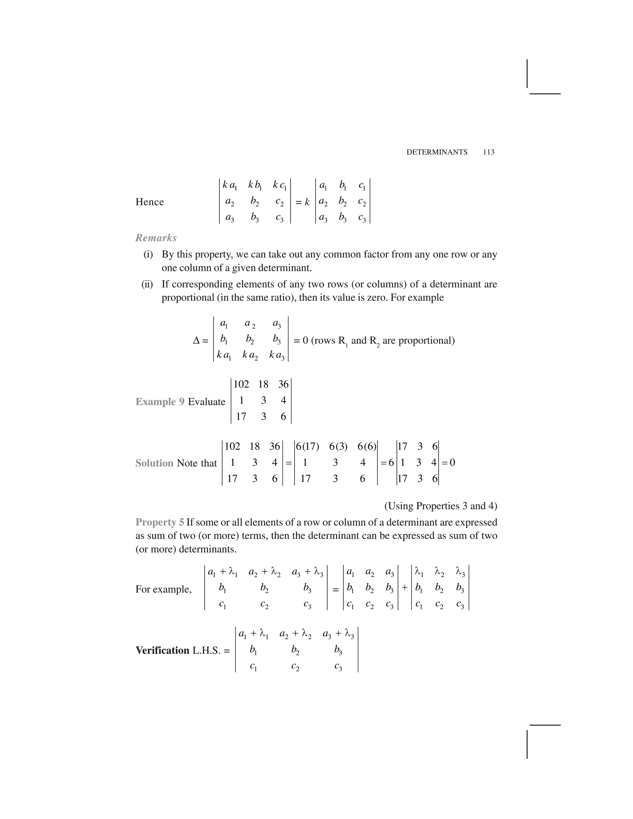
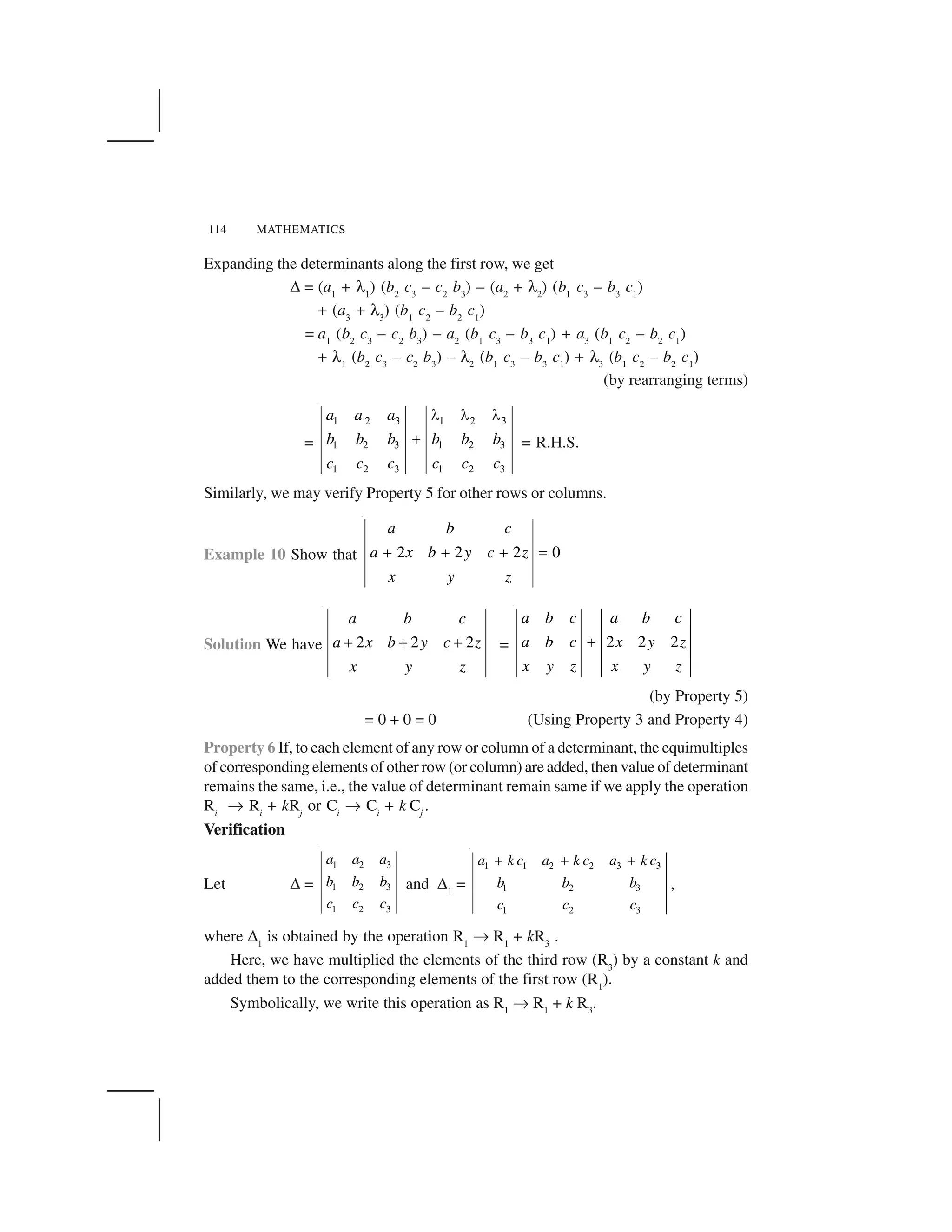

![116 MATHEMATICS
Example 12 Without expanding, prove that
✆ = 0
1 1 1
x y y z z x
z x y
✁
Solution Applying R1
✄ R1
+ R2
to ✆, we get
✆ =
1 1 1
x y z x y z x y z
z x y
✂ ✂ ✂ ✂ ✂ ✂
Since the elements of R1
and R3
are proportional, ✆ = 0.
Example 13 Evaluate
✆ =
1
1
1
a bc
b ca
c ab
Solution Applying R2
✄ R2
– R1
and R3
✄ R3
– R1
, we get
✆ =
1
0 ( )
0 ( )
a bc
b a c a b
c a b a c
☎ ☎
☎ ☎
Taking factors (b – a) and (c – a) common from R2
and R3
, respectively, we get
✆ =
1
( ) ( ) 0 1 –
0 1 –
a bc
b a c a c
b
✝ ✝
= (b – a) (c – a) [(– b + c)] (Expanding along first column)
= (a – b) (b – c) (c – a)
Example 14 Prove that 4
b c a a
b c a b abc
c c a b
✁
Solution Let ✆ =
b c a a
b c a b
c c a b
✂
✂
✂](https://image.slidesharecdn.com/ncert-class-12-mathematics-part-1-161112165946/75/Ncert-class-12-mathematics-part-1-119-2048.jpg)
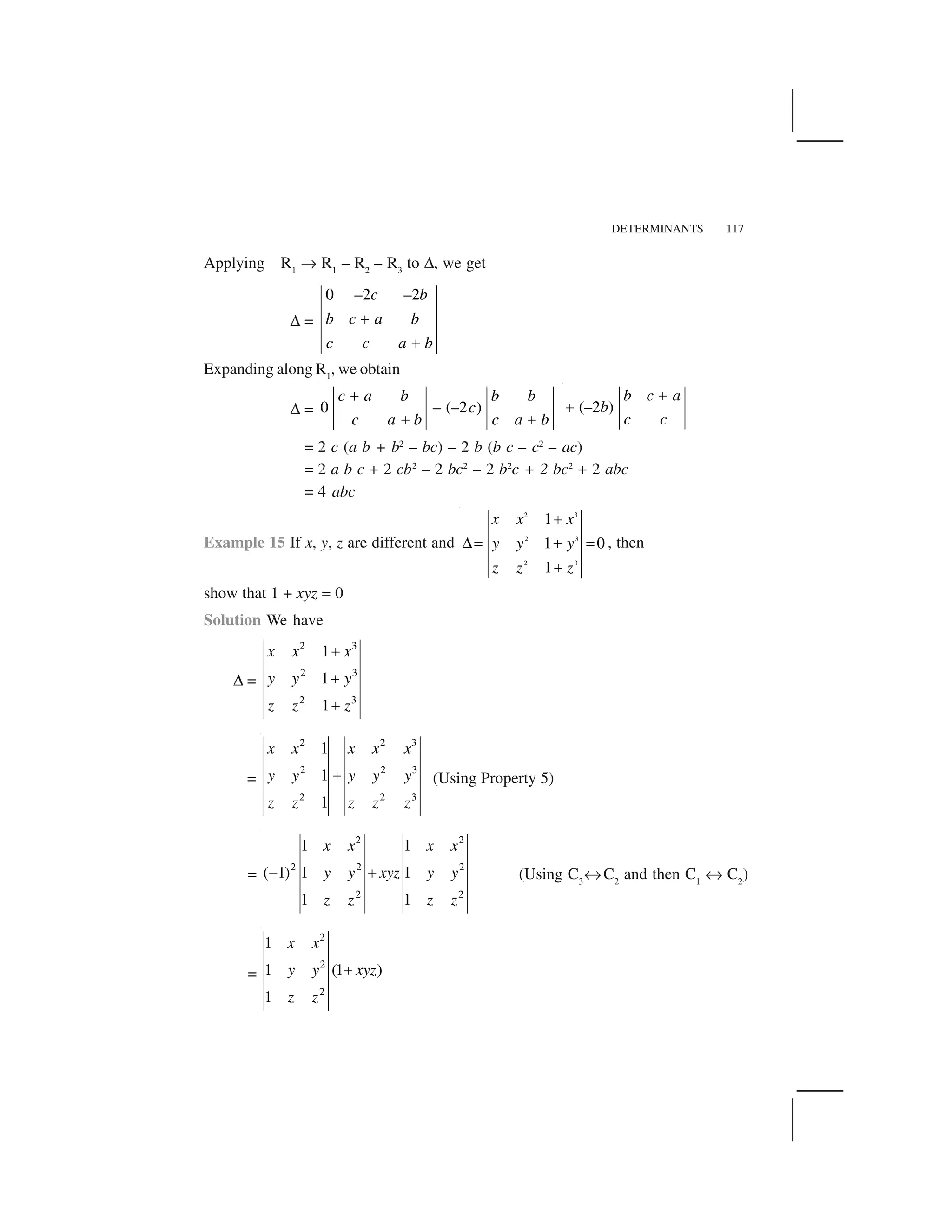
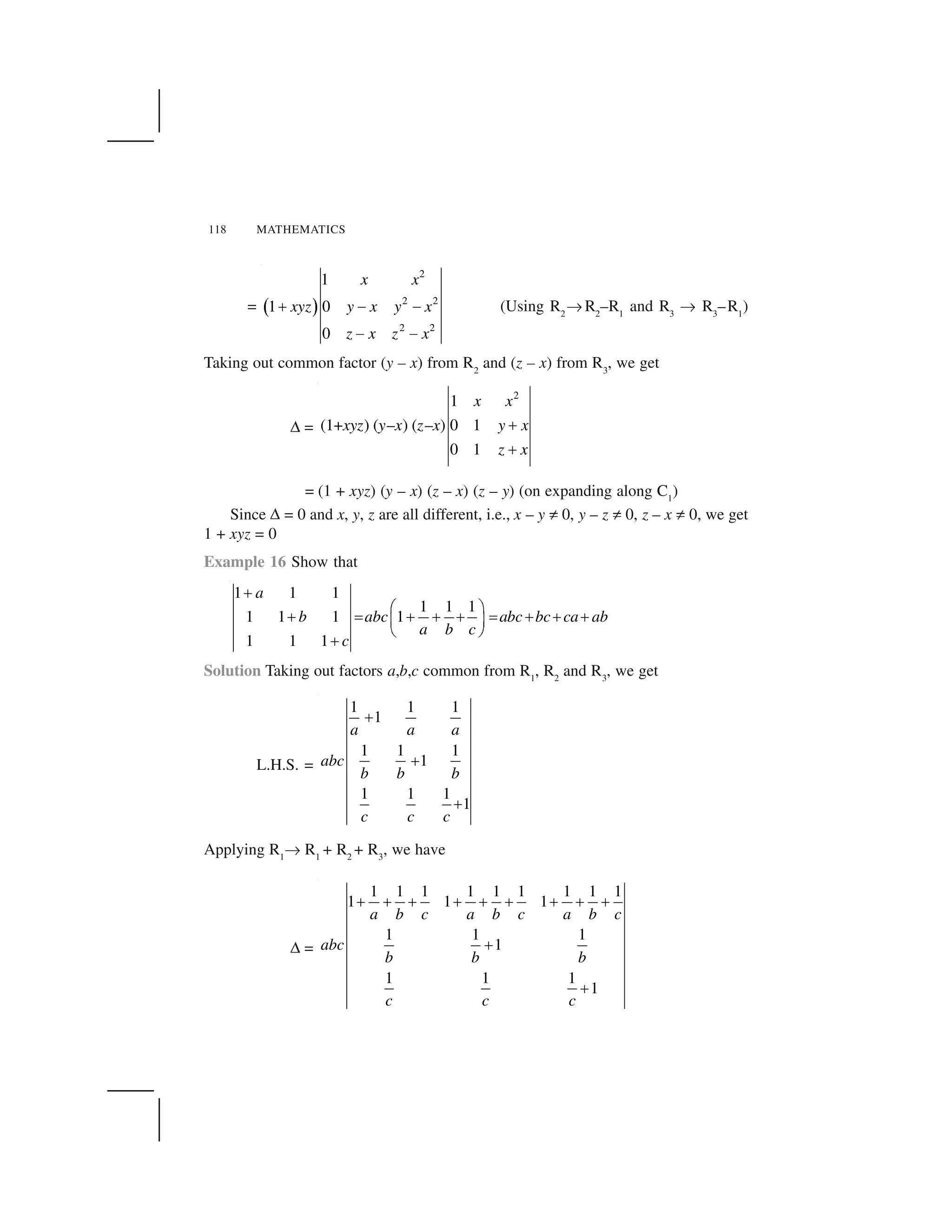
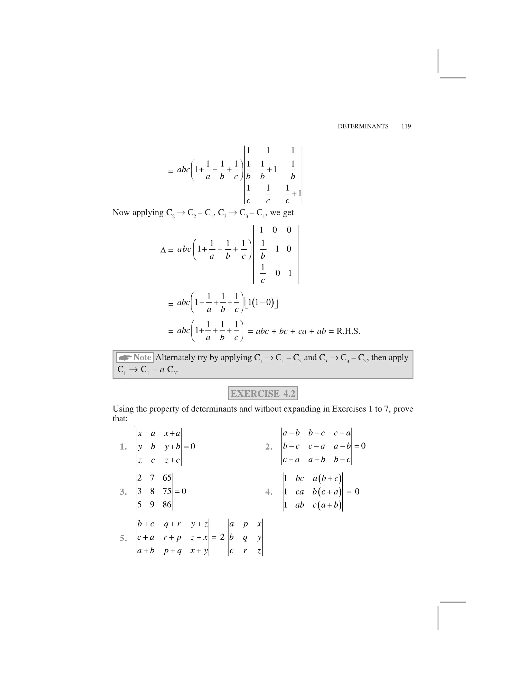
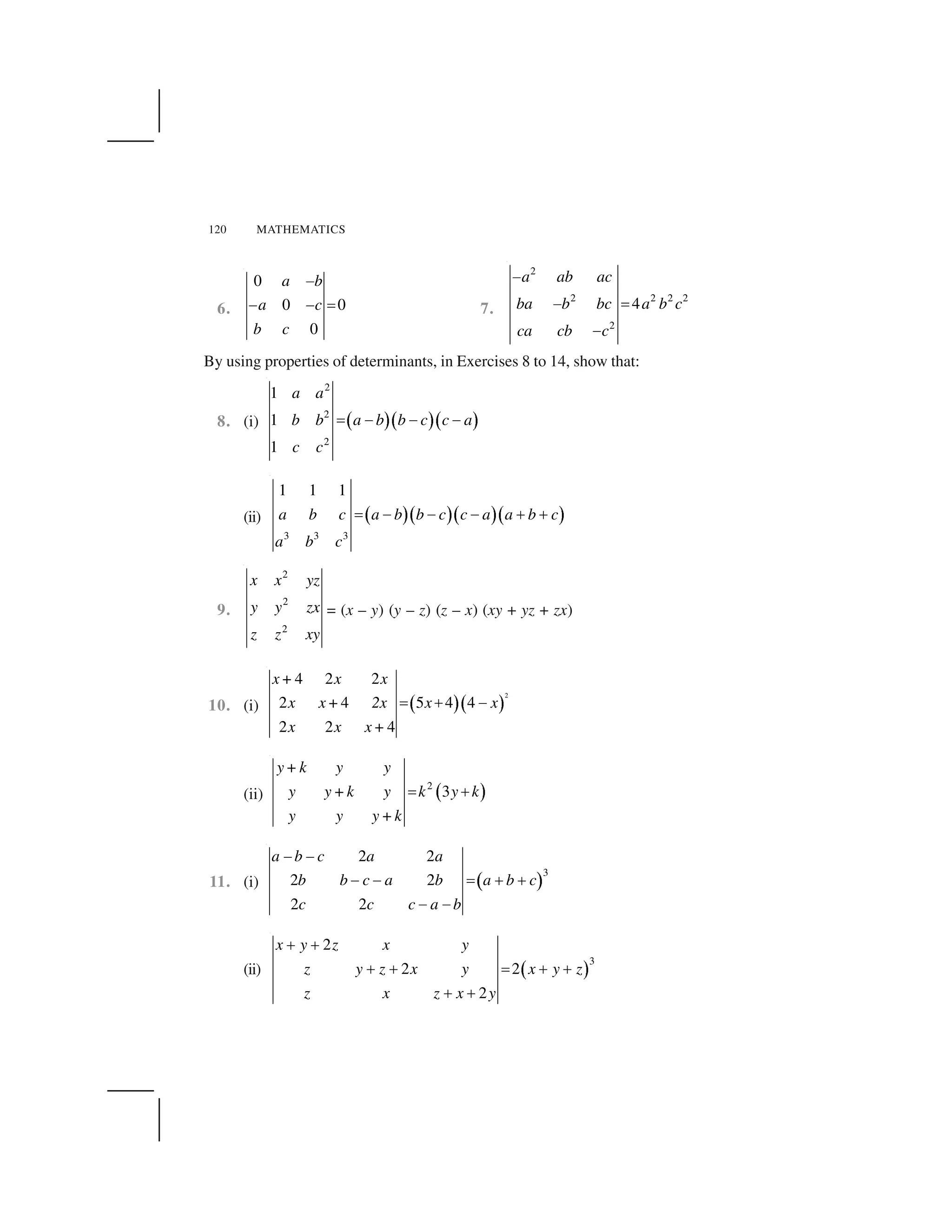
![DETERMINANTS 121
12. ✁
2
22 3
2
1
1 1
1
x x
x x x
x x
✂ ✄
13. ☎ ✆
2 2
32 2 2 2
2 2
1 2 2
2 1 2 1
2 2 1
a b ab b
ab a b a a b
b a a b
✝ ✄ ✄
✄ ✝ ✂ ✝ ✝
✄ ✄ ✄
14.
2
2 2 2 2
2
1
1 1
1
a ab ac
ab b bc a b c
ca cb c
✝
✝ ✂ ✝ ✝ ✝
✝
Choose the correct answer in Exercises 15 and 16.
15. Let A be a square matrix of order 3 × 3, then |kA| is equal to
(A) k| A | (B) k2
| A | (C) k3
| A | (D) 3k | A |
16. Which of the following is correct
(A) Determinant is a square matrix.
(B) Determinant is a number associated to a matrix.
(C) Determinant is a number associated to a square matrix.
(D) None of these
4.4 Area of a Triangle
In earlier classes, we have studied that the area of a triangle whose vertices are
(x1
, y1
), (x2
, y2
) and (x3
, y3
), is given by the expression
1
2
[x1
(y2
–y3
) + x2
(y3
–y1
) +
x3
(y1
–y2
)]. Now this expression can be written in the form of a determinant as
✞ =
1 1
2 2
3 3
1
1
1
2
1
x y
x y
x y
... (1)
Remarks
(i) Since area is a positive quantity, we always take the absolute value of the
determinant in (1).](https://image.slidesharecdn.com/ncert-class-12-mathematics-part-1-161112165946/75/Ncert-class-12-mathematics-part-1-124-2048.jpg)
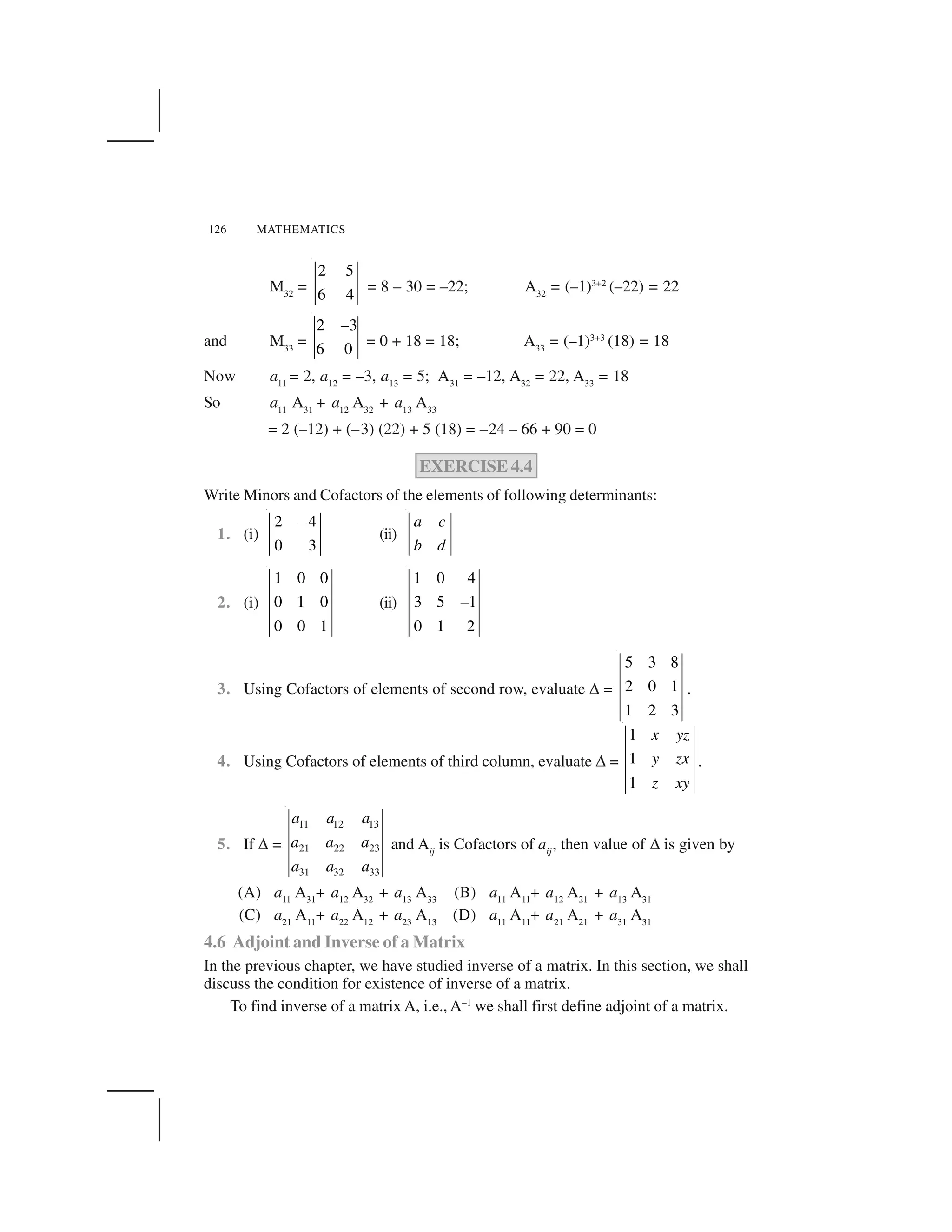
![DETERMINANTS 127
4.6.1 Adjoint of a matrix
Definition 3 The adjoint of a square matrix A = [aij
]n × n
is defined as the transpose of
the matrix [Aij
]n × n
, where Aij
is the cofactor of the element aij
. Adjoint of the matrix A
is denoted by adj A.
Let
11 12 13
21 22 23
31 32 33
A =
a a a
a a a
a a a
✁
✂ ✄
✂ ✄
✂ ✄☎ ✆
Then
11 12 13
21 22 23
31 32 33
A A A
A =Transposeof A A A
A A A
adj
✁
✂ ✄
✂ ✄
✂ ✄☎ ✆
11 21 31
12 22 32
13 23 33
A A A
= A A A
A A A
✁
✂ ✄
✂ ✄
✂ ✄☎ ✆
Example 23
2 3
Find A for A =
1 4
adj
✝ ✞
✟ ✠
✡ ☛
Solution We have A11
= 4, A12
= –1, A21
= –3, A22
= 2
Hence adj A =
11 21
12 22
A A 4 –3
=
A A –1 2
☞ ✌ ☞ ✌
✍ ✎ ✍ ✎
✏ ✑✏ ✑
Remark For a square matrix of order 2, given by
A =
11 12
21 22
a a
a a
✝ ✞
✟ ✠
✡ ☛
The adj A can also be obtained by interchanging a11
and a22
and by changing signs
of a12
and a21
, i.e.,
We state the following theorem without proof.
Theorem 1 If A be any given square matrix of order n, then
A(adj A) = (adj A) A = ❆ ✒ ,
where I is the identity matrix of order n](https://image.slidesharecdn.com/ncert-class-12-mathematics-part-1-161112165946/75/Ncert-class-12-mathematics-part-1-130-2048.jpg)
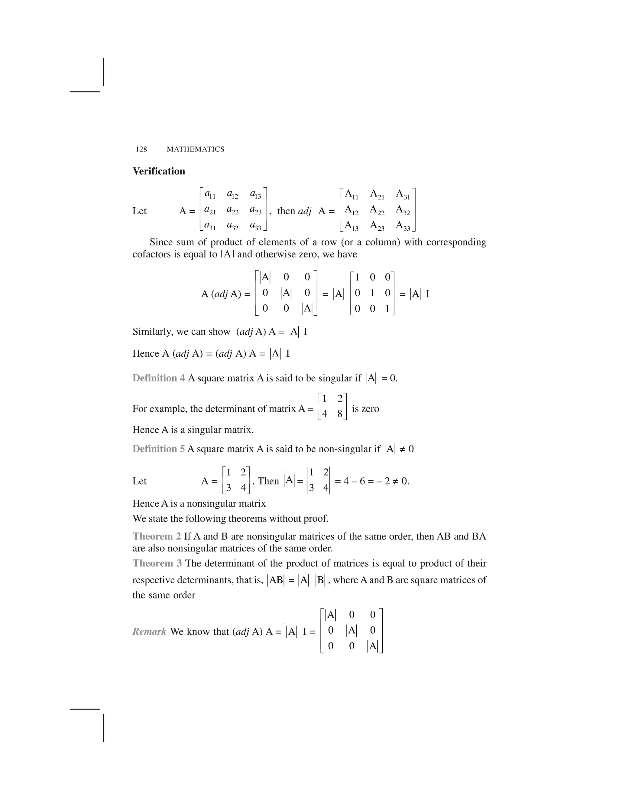
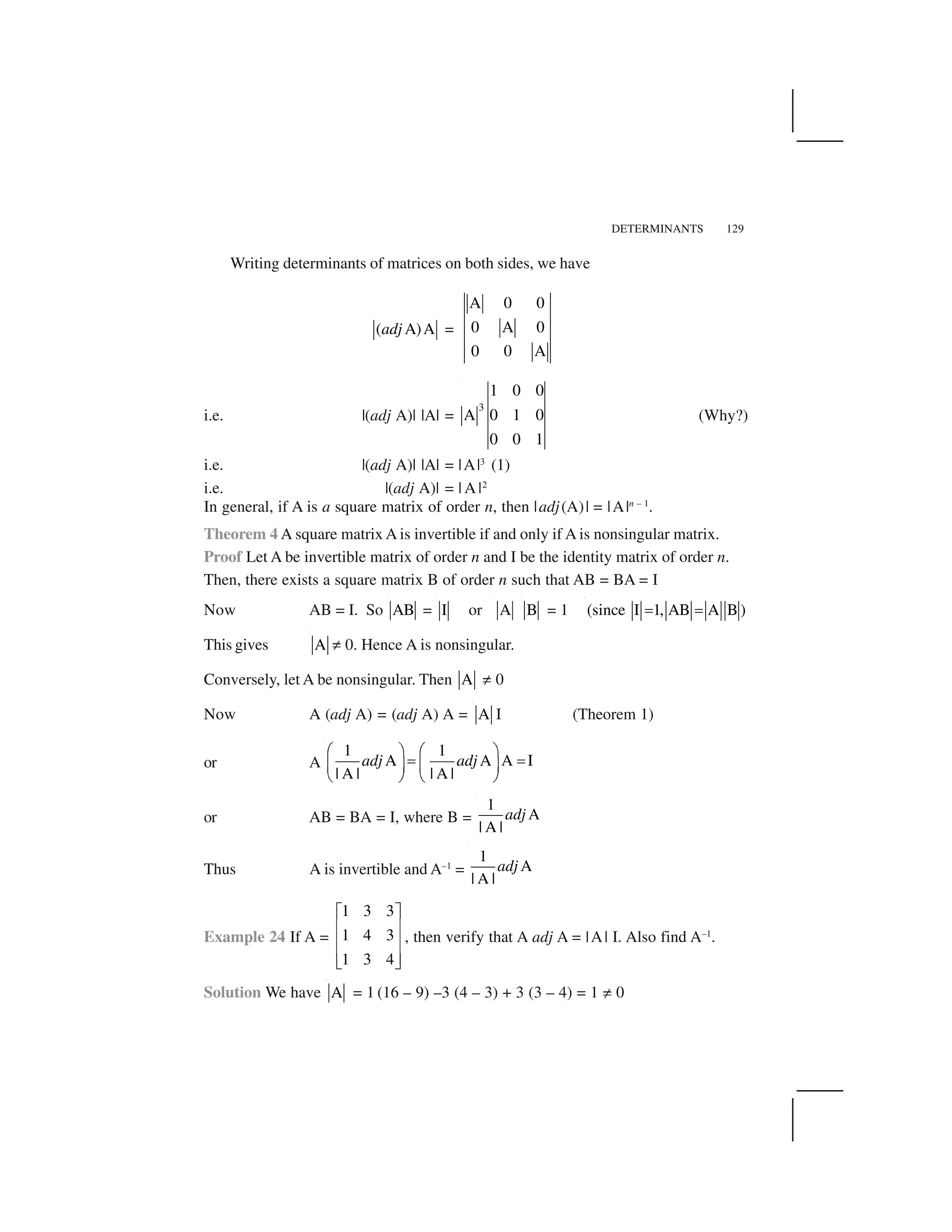
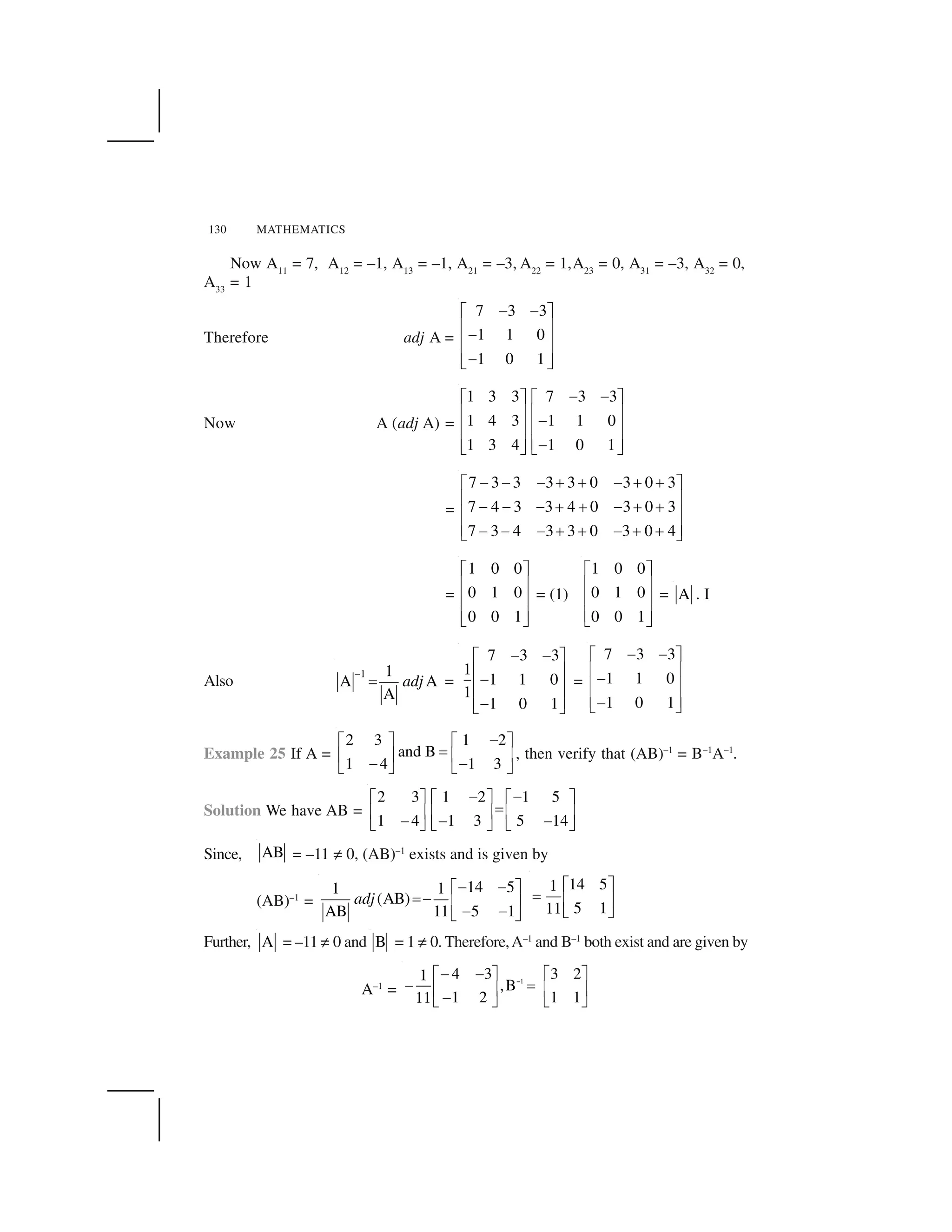
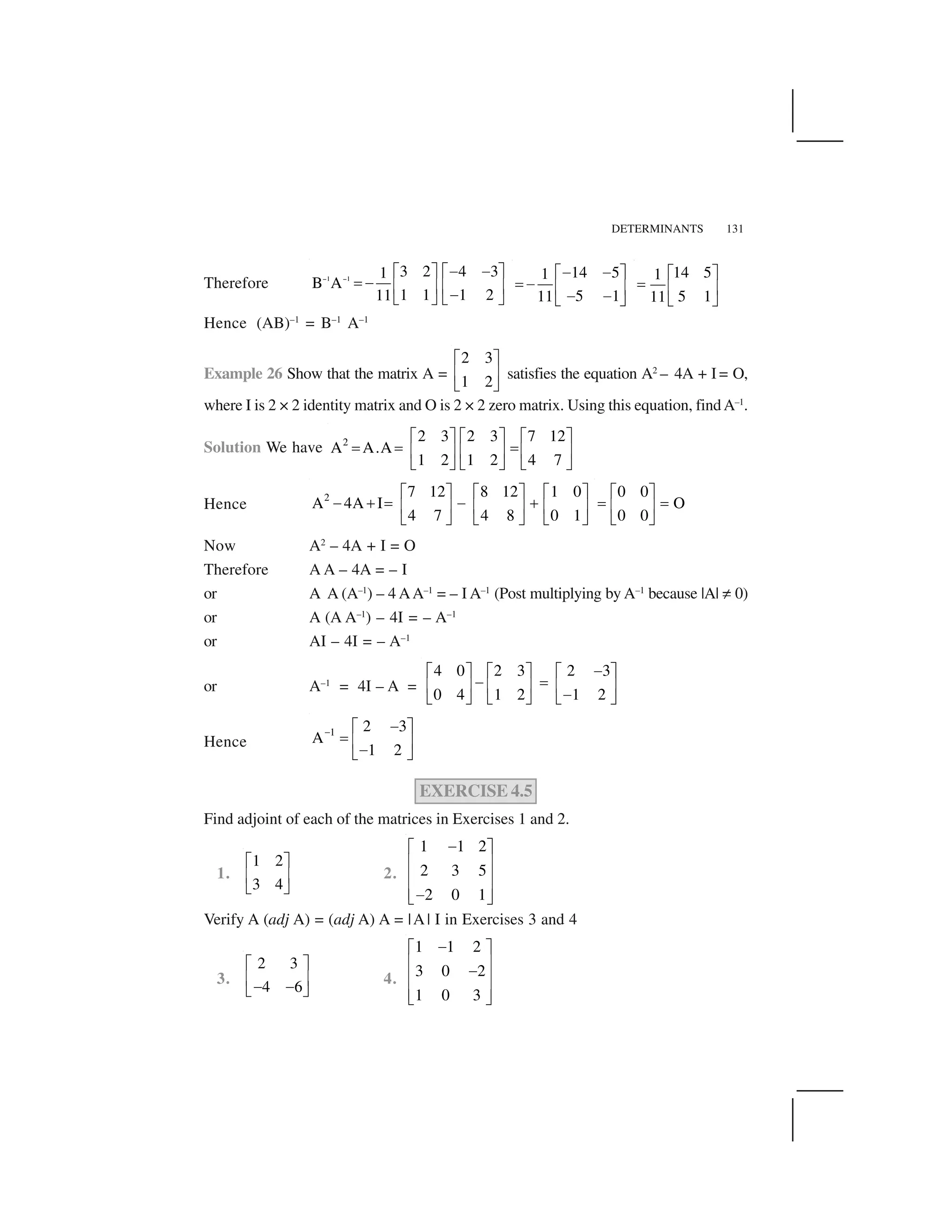
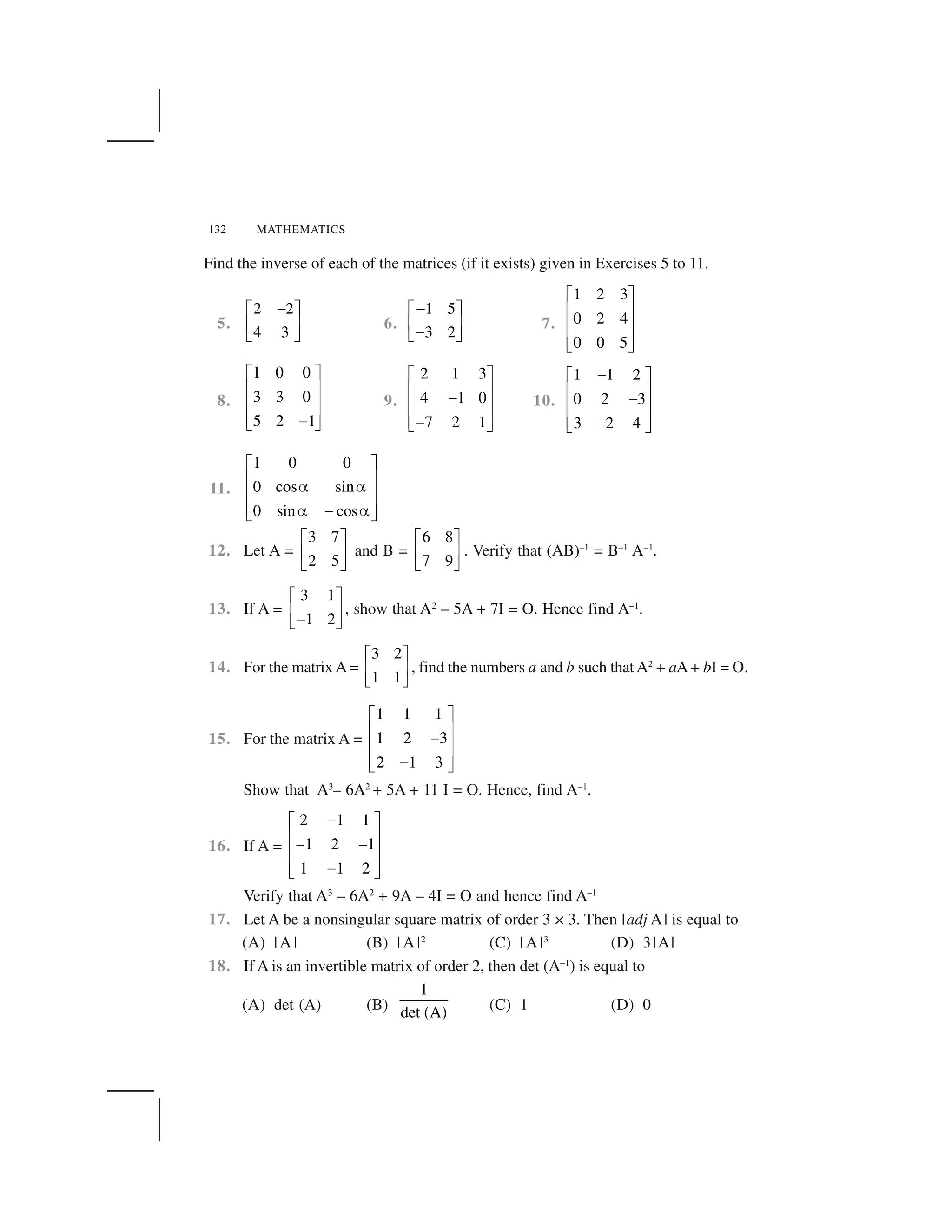
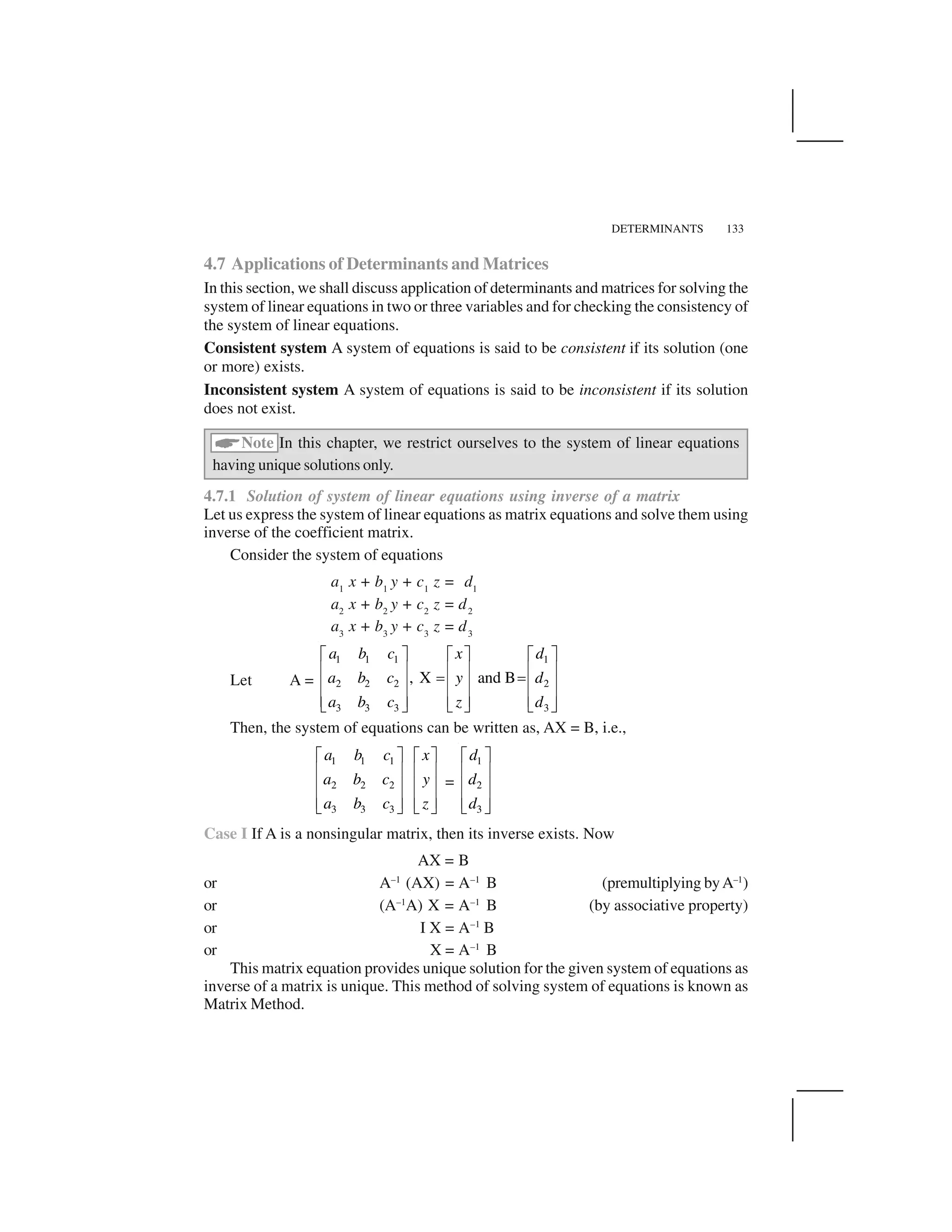
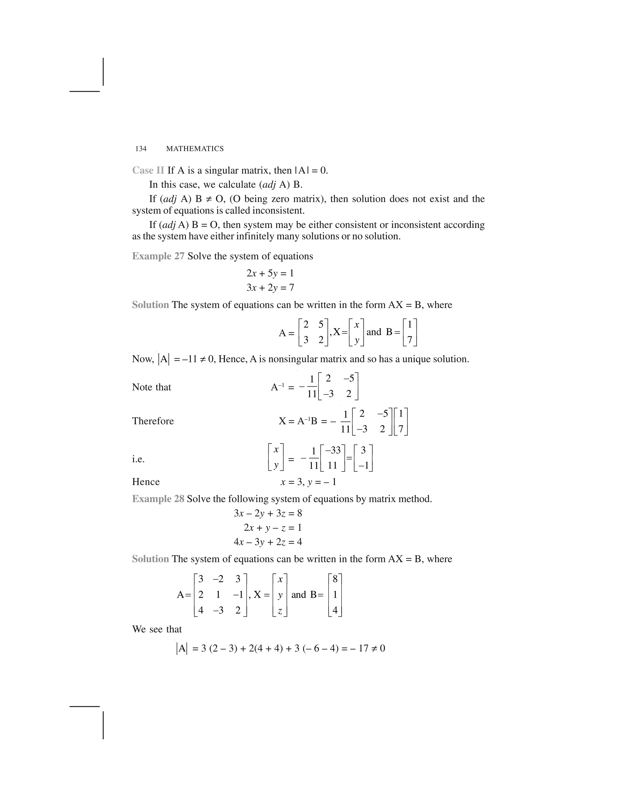
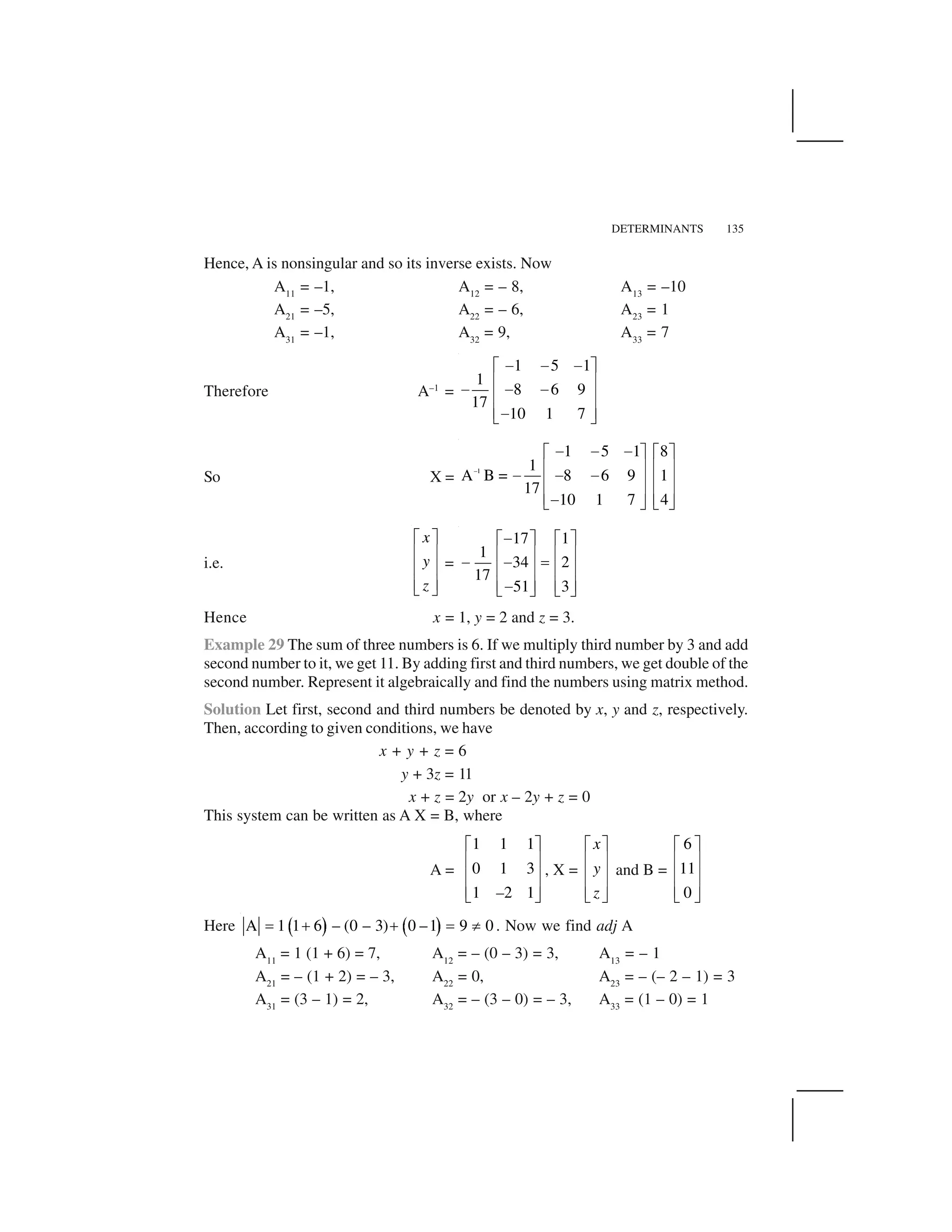
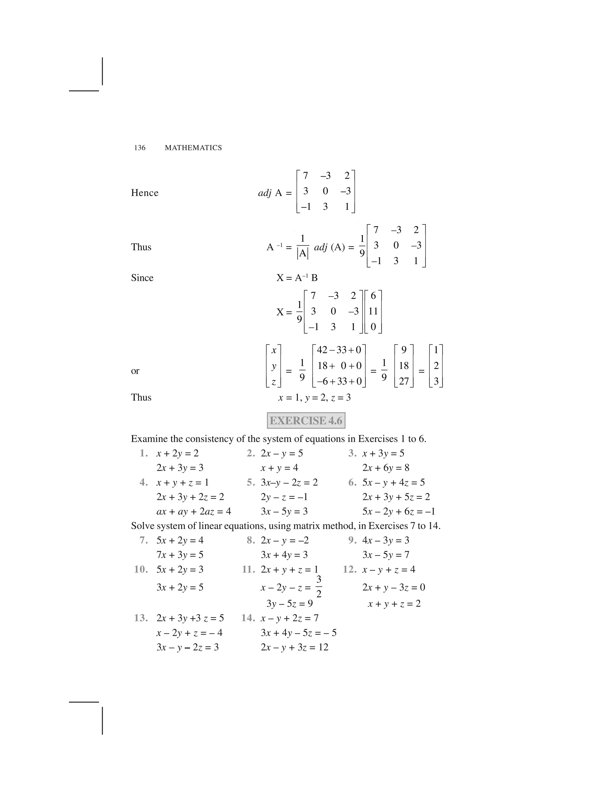
![DETERMINANTS 137
15. If A =
2 –3 5
3 2 – 4
1 1 –2
✁
✂ ✄
✂ ✄
✂ ✄☎ ✆
, find A–1
. Using A–1
solve the system of equations
2x – 3y + 5z = 11
3x + 2y – 4z = – 5
x + y – 2z = – 3
16. The cost of 4 kg onion, 3 kg wheat and 2 kg rice is Rs 60. The cost of 2 kg onion,
4 kg wheat and 6 kg rice is Rs 90. The cost of 6 kg onion 2 kg wheat and 3 kg
rice is Rs 70. Find cost of each item per kg by matrix method.
Miscellaneous Examples
Example 30 If a, b, c are positive and unequal, show that value of the determinant
✝ =
a b c
b c a
c a b
is negative.
Solution Applying C1
✞ C1
+ C2
+ C3
to the given determinant, we get
✝ =
a b c b c
a b c c a
a b c a b
✟ ✟
✟ ✟
✟ ✟
= (a + b + c)
1
1
1
b c
c a
a b
= (a + b + c)
1
0 – –
0 – –
b c
c b a c
a b b c
(ApplyingR2
✞ R2
–R1
,andR3
✞R3
–R1
)
= (a + b + c) [(c – b) (b – c) – (a – c) (a – b)] (Expanding along C1
)
= (a + b + c)(– a2
– b2
– c2
+ ab + bc + ca)
=
1
2
–
(a + b + c) (2a2
+ 2b2
+ 2c2
– 2ab – 2bc – 2ca)
=
1
2
–
(a + b + c) [(a – b)2
+ (b – c)2
+ (c – a)2
]
which is negative (since a + b + c > 0 and (a – b)2
+ (b – c)2
+ (c – a)2
> 0)](https://image.slidesharecdn.com/ncert-class-12-mathematics-part-1-161112165946/75/Ncert-class-12-mathematics-part-1-140-2048.jpg)
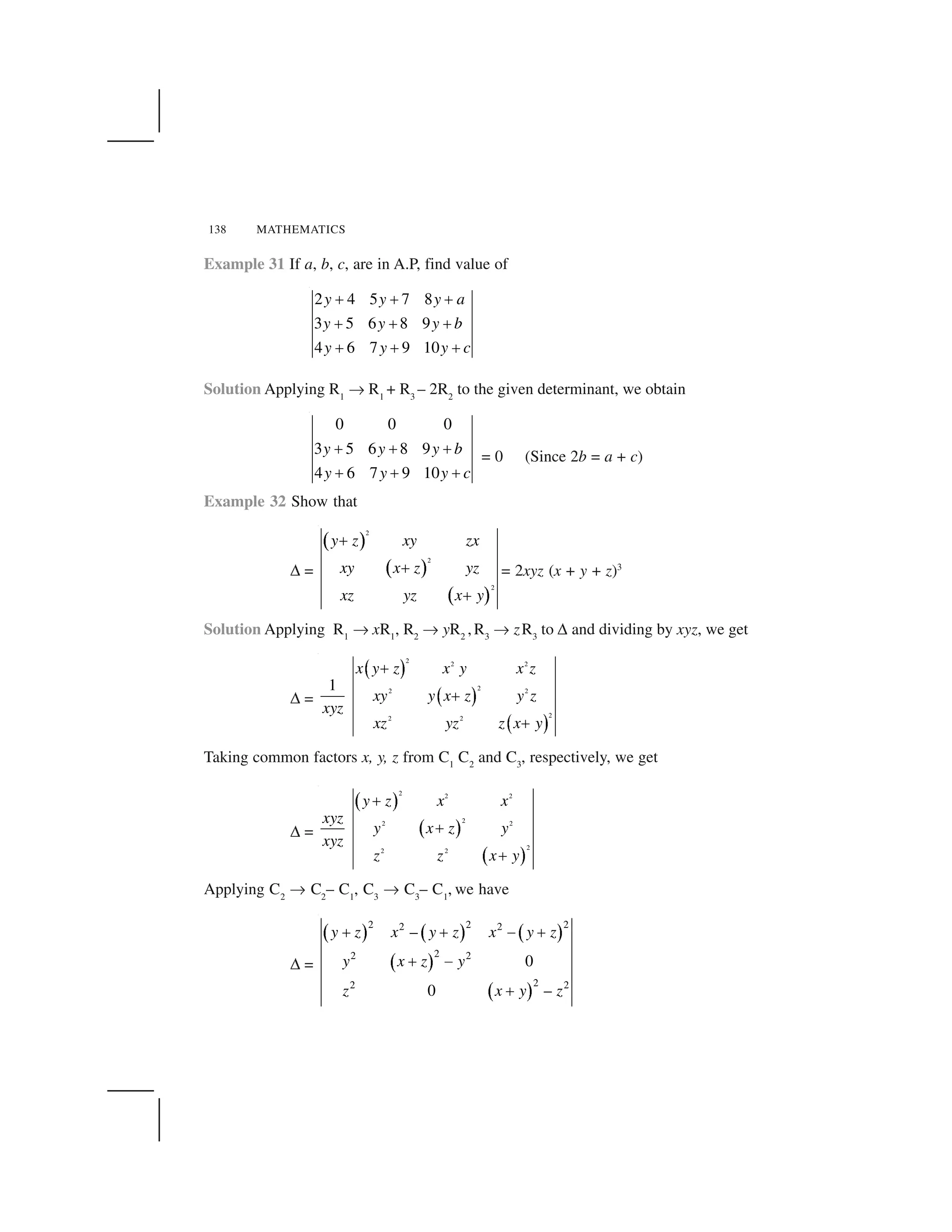
![DETERMINANTS 139
Taking common factor (x + y + z) from C2
and C3
, we have
✆ = (x + y + z)2
✁ ✁ ✁
✁
✁
2
2
2
y
0
0
z x – y z x – y z
y x z – y
z x y – z
✂ ✂ ✂
✂
✂
Applying R1
✄ R1
– (R2
+ R3
), we have
✆ = (x + y + z)2 2
2
2 2 2
+ 0
0 – z
yz – z – y
y x y z
z x y
☎
✝
Applying C2
✄ (C2
+
1
y
C1
) and 3 3 1
1
C C C
✞ ✟
✠ ✡☛ ☞
✌ ✍z
, we get
✆ = (x + y + z)2
2
2
2
2
2 0 0
✎
✎
yz
y
y x z
z
z
z x y
y
Finally expanding along R1
, we have
✆ = (x + y + z)2
(2yz) [(x + z) (x + y) – yz] = (x + y + z)2
(2yz) (x2
+ xy + xz)
= (x + y + z)3
(2xyz)
Example 33 Use product
1 1 2 2 0 1
0 2 3 9 2 3
3 2 4 6 1 2
✏ ✑ ✏ ✑
✒ ✓ ✒ ✓
✒ ✓ ✒ ✓
✒ ✓ ✒ ✓✔ ✕ ✔ ✕
– –
– –
– –
to solve the system of equations
x – y + 2z = 1
2y – 3z = 1
3x – 2y + 4z = 2
Solution Consider the product
1 1 2 2 0 1
0 2 3 9 2 3
3 2 4 6 1 2
– –
– –
– –
✖ ✗ ✖ ✗
✘ ✙ ✘ ✙
✘ ✙ ✘ ✙
✘ ✙ ✘ ✙✚ ✛ ✚ ✛](https://image.slidesharecdn.com/ncert-class-12-mathematics-part-1-161112165946/75/Ncert-class-12-mathematics-part-1-142-2048.jpg)
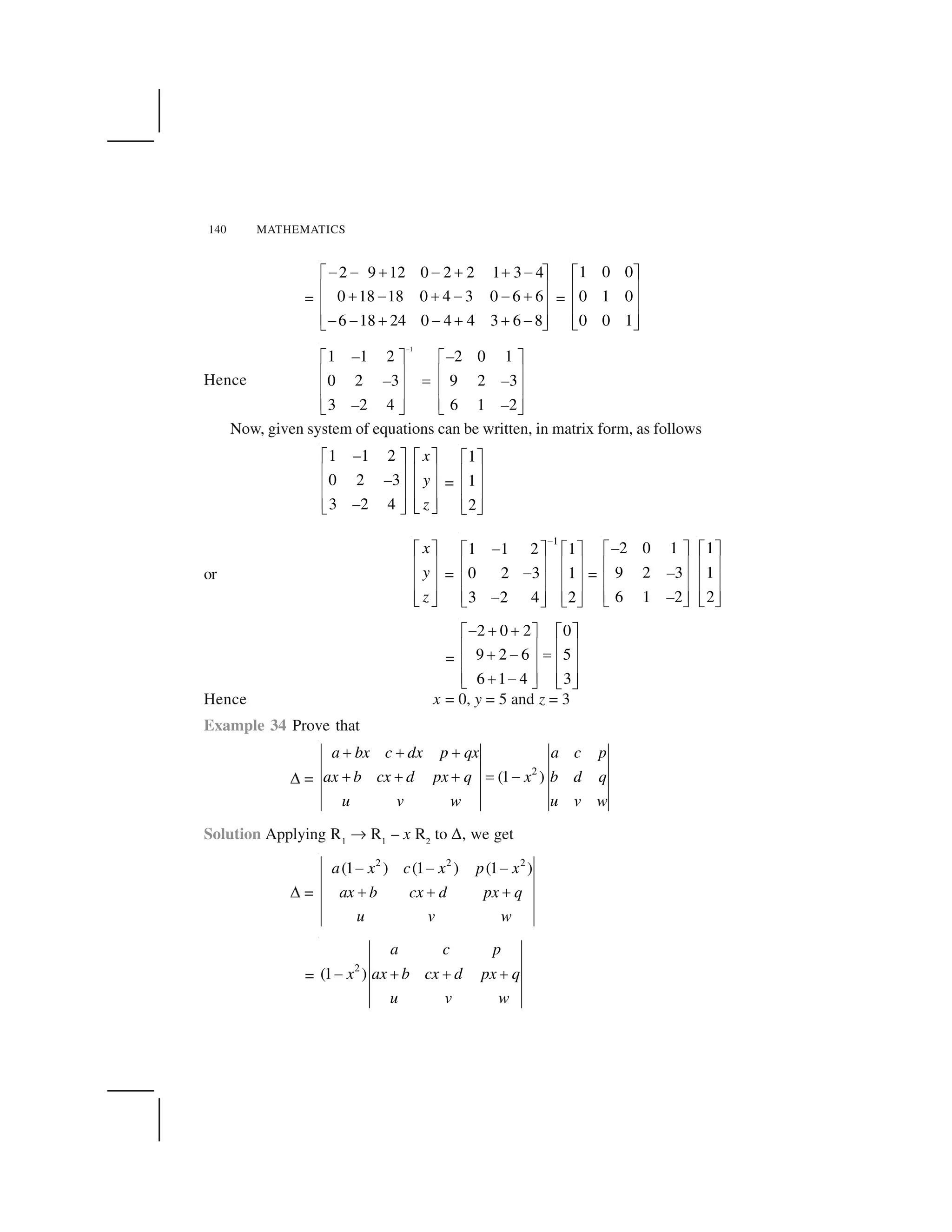
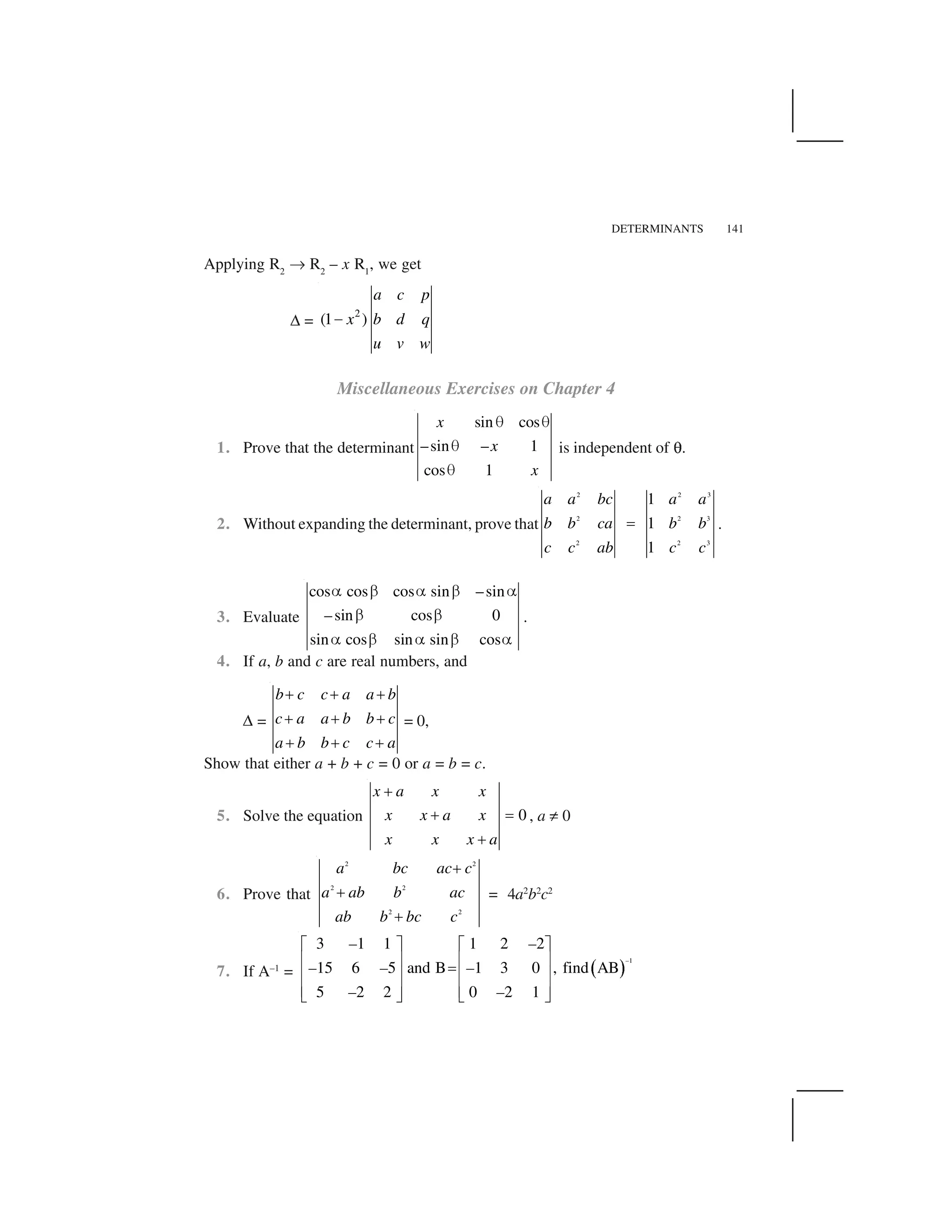
![142 MATHEMATICS
8. Let A =
1 2 1
2 3 1
1 1 5
✁
✂ ✄
✂ ✄
✂ ✄☎ ✆
–
– . Verify that
(i) [adj A]–1
= adj (A–1
) (ii) (A–1
)–1
= A
9. Evaluate
x y x y
y x y x
x y x y
✝
✝
✝
10. Evaluate
1
1
1
x y
x y y
x x+ y
✝
Using properties of determinants in Exercises 11 to 15, prove that:
11.
2
2
2
✞ ✞ ✟ ✠ ✡
✟ ✟ ✡ ✠ ✞
✡ ✡ ✞ ✠ ✟
= (☛ – ✌) (✌ – ☞) (☞ – ☛) (☞ + ☛ + ✌)
12.
2 3
2 3
2 3
1
1
1
✍
✍
✍
x x px
y y py
z z pz
= (1 + pxyz) (x – y) (y – z) (z – x), where p is any scalar.
13.
3
3
a 3c
a – a+b – a+c
–b a b –b c
– c – c+b
✠ ✠
✠
= 3(a + b + c) (ab + bc + ca)
14.
1 1 1
2 3 2 4 3 2
3 6 3 10 6 3
p p q
p p q
p p q
✝ ✝ ✝
✝ ✝ ✝
✝ ✝ ✝
= 1 15.
✎ ✏
✎ ✏
✎ ✏
sin cos cos
sin cos cos 0
sin cos cos
✑ ✑ ✑ ✒ ✓
✔ ✔ ✔ ✒ ✓ ✕
✖ ✖ ✖ ✒ ✓
16. Solve the system of equations
2 3 10
4✗ ✗ ✘
x y z](https://image.slidesharecdn.com/ncert-class-12-mathematics-part-1-161112165946/75/Ncert-class-12-mathematics-part-1-145-2048.jpg)
![DETERMINANTS 143
4 6 5
1 ✁–
x y z
6 9 20
2 ✁–
x y z
Choose the correct answer in Exercise 17 to 19.
17. If a, b, c, are in A.P, then the determinant
2 3 2
3 4 2
4 5 2
x x x a
x x x b
x x x c
✂ ✂ ✂
✂ ✂ ✂
✂ ✂ ✂
is
(A) 0 (B) 1 (C) x (D) 2x
18. If x, y, z are nonzero real numbers, then the inverse of matrix
0 0
A 0 0
0 0
x
y
z
✄ ☎
✆ ✝✞ ✆ ✝
✆ ✝✟ ✠
is
(A)
1
1
1
0 0
0 0
0 0
x
y
z
✡
✡
✡
☛ ☞
✌ ✍
✌ ✍
✌ ✍
✎ ✏
(B)
1
1
1
0 0
0 0
0 0
x
xyz y
z
✡
✡
✡
☛ ☞
✌ ✍
✌ ✍
✌ ✍
✎ ✏
(C)
0 0
1
0 0
0 0
x
y
xyz
z
✑ ✒
✓ ✔
✓ ✔
✓ ✔✕ ✖
(D)
1 0 0
1
0 1 0
0 0 1
xyz
✄ ☎
✆ ✝
✆ ✝
✆ ✝✟ ✠
19. Let A =
1 sin 1
sin 1 sin
1 sin 1
✗✑ ✒
✓ ✔✘ ✗ ✗✓ ✔
✓ ✔✘ ✘ ✗✕ ✖
, where 0 ✙ ✚ ✙ 2✛. Then
(A) Det (A) = 0 (B) Det (A) ✜ (2, ✢)
(C) Det (A) ✜ (2, 4) (D) Det (A) ✜ [2, 4]](https://image.slidesharecdn.com/ncert-class-12-mathematics-part-1-161112165946/75/Ncert-class-12-mathematics-part-1-146-2048.jpg)
![144 MATHEMATICS
Summary
Determinant of a matrix A = [a11
]1×1
is given by |a11
| = a11
Determinant of a matrix 11 12
21 22
A
a a
a a
✁ ✂✄☎ ✆✝ ✞
is given by
11 12
21 22
A
a a
a a
✄ = a11
a22
– a12
a21
Determinant of a matrix
1 1 1
2 2 2
3 3 3
A
a b c
a b c
a b c
✟ ✠✡ ☛☞✡ ☛✡ ☛✌ ✍
is given by (expanding along R1
)
1 1 1
2 2 2 2 2 2
2 2 2 1 1 1
3 3 3 3 3 3
3 3 3
A
a b c
b c a c a b
a b c a b c
b c a c a b
a b c
✎ ✎ ✏ ✑
For any square matrix A, the |A| satisfy following properties.
|A✒| = |A|, where A✒ = transpose of A.
If we interchange any two rows (or columns), then sign of determinant
changes.
If any two rows or any two columns are identical or proportional, then value
of determinant is zero.
If we multiply each element of a row or a column of a determinant by constant
k, then value of determinant is multiplied by k.
Multiplying a determinant by k means multiply elements of only one row
(or one column) by k.
If 3
3 3A [ ] ,then .A Aija k k✓✔ ✔
If elements of a row or a column in a determinant can be expressed as sum
of two or more elements, then the given determinant can be expressed as
sum of two or more determinants.
If to each element of a row or a column of a determinant the equimultiples of
corresponding elements of other rows or columns are added, then value of
determinant remains same.](https://image.slidesharecdn.com/ncert-class-12-mathematics-part-1-161112165946/75/Ncert-class-12-mathematics-part-1-147-2048.jpg)
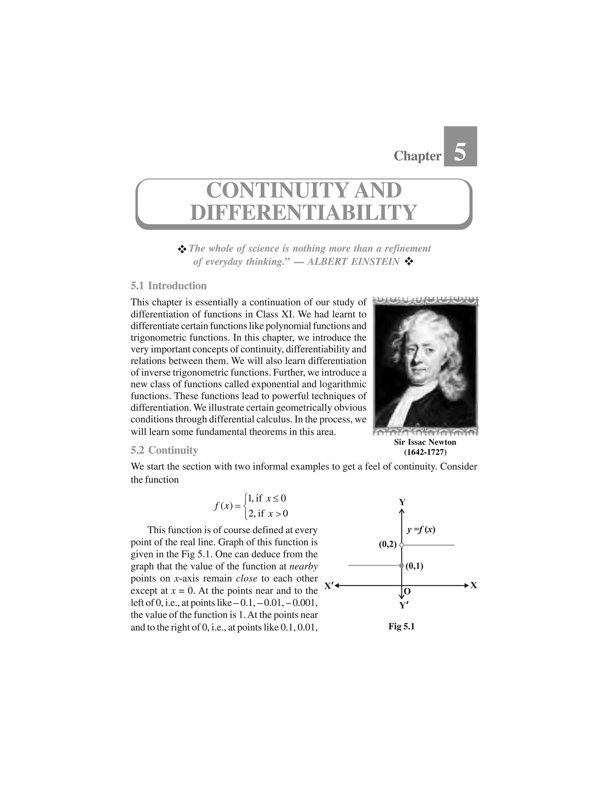
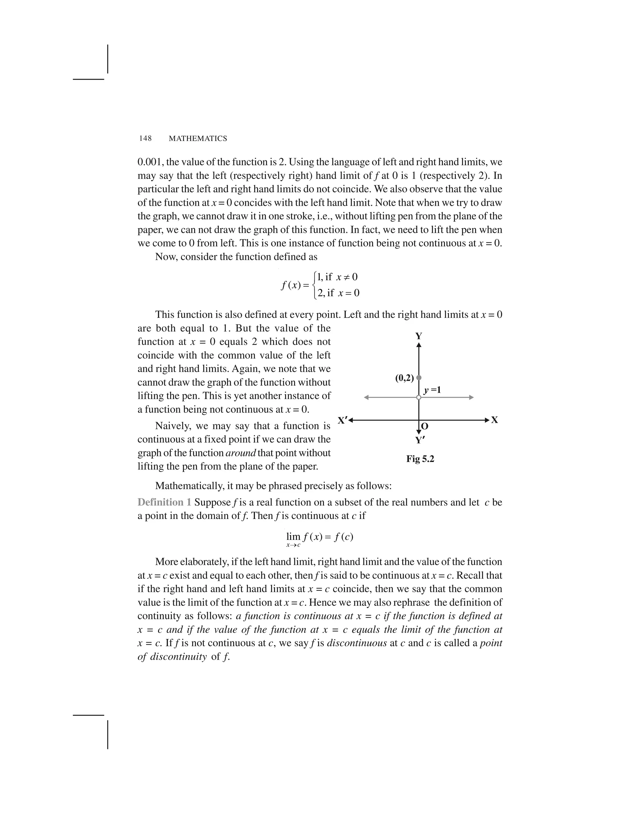
![MATHEMATICS150
Solution The function is defined at x = 0 and its value at x = 0 is 1. When x ✂ 0, the
function is given by a polynomial. Hence,
0
lim ( )
x
f x
=
3 3
0
lim ( 3) 0 3 3
x
x
✁
✄ ☎ ✄ ☎
Since the limit of f at x = 0 does not coincide with f(0), the function is not continuous
at x = 0. It may be noted that x = 0 is the only point of discontinuity for this function.
Example 5 Check the points where the constant function f (x) = k is continuous.
Solution The function is defined at all real numbers and by definition, its value at any
real number equals k. Let c be any real number. Then
lim ( )
x c
f x
= lim
x c
k k
✆
Since f(c) = k = lim
x c✝ f (x) for any real number c, the function f is continuous at
every real number.
Example 6 Prove that the identity function on real numbers given by f (x) = x is
continuous at every real number.
Solution The function is clearly defined at every point and f (c) = c for every real
number c. Also,
lim ( )
x c
f x
✝ = lim
x c
x c
✝ ✞
Thus, lim
x c f (x) = c = f(c) and hence the function is continuous at every real number.
Having defined continuity of a function at a given point, now we make a natural
extension of this definition to discuss continuity of a function.
Definition 2 A real function f is said to be continuous if it is continuous at every point
in the domain of f.
This definition requires a bit of elaboration. Suppose f is a function defined on a
closed interval [a, b], then for f to be continuous, it needs to be continuous at every
point in [a, b] including the end points a and b. Continuity of f at a means
lim ( )
x a
f x✟✠
= f (a)
and continuity of f at b means
–
lim ( )
x b
f x
✠ = f(b)
Observe that lim ( )
x a
f x✡✠
and lim ( )
x b
f x✟✠
do not make sense. As a consequence
of this definition, if f is defined only at one point, it is continuous there, i.e., if the
domain of f is a singleton, f is a continuous function.](https://image.slidesharecdn.com/ncert-class-12-mathematics-part-1-161112165946/75/Ncert-class-12-mathematics-part-1-153-2048.jpg)
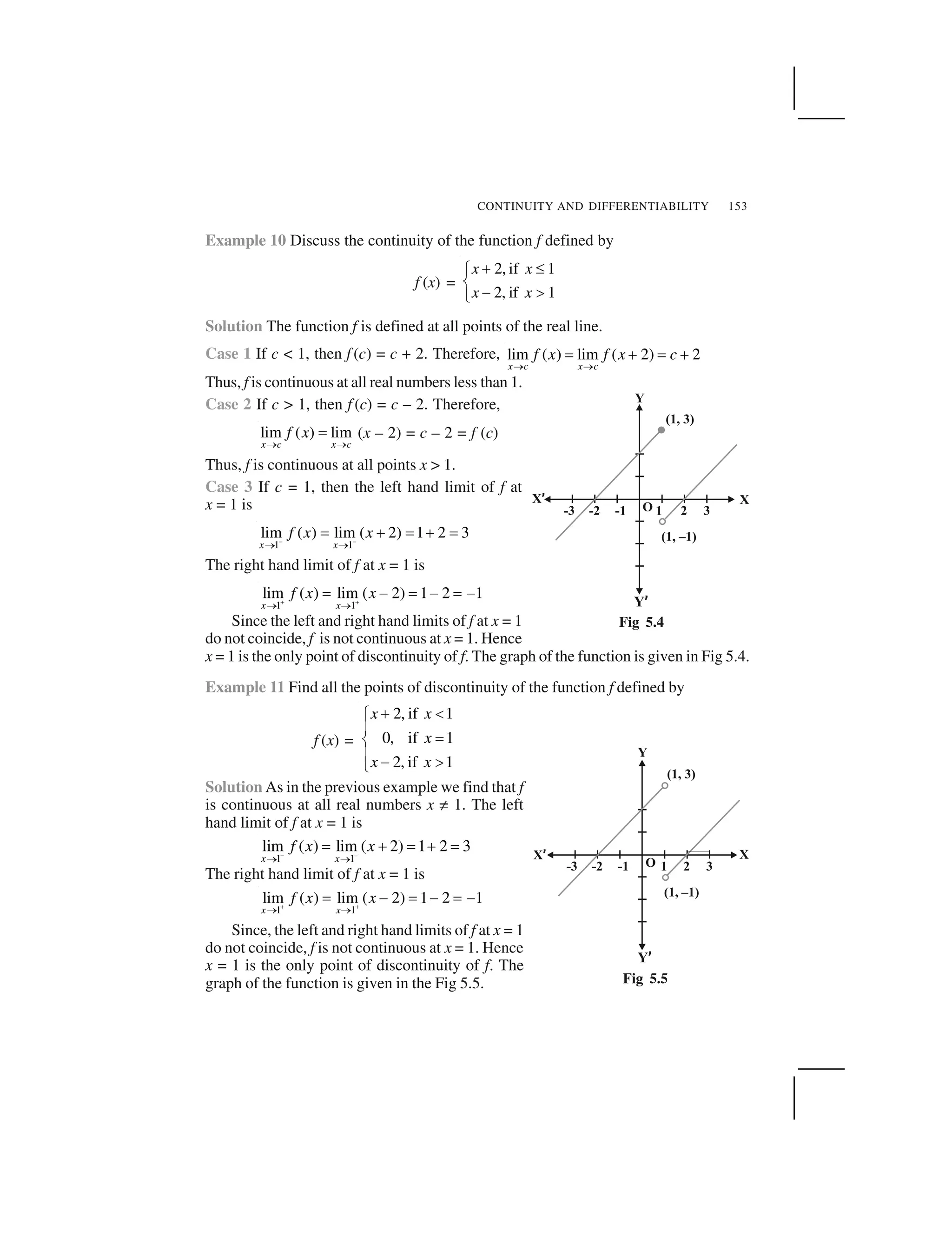
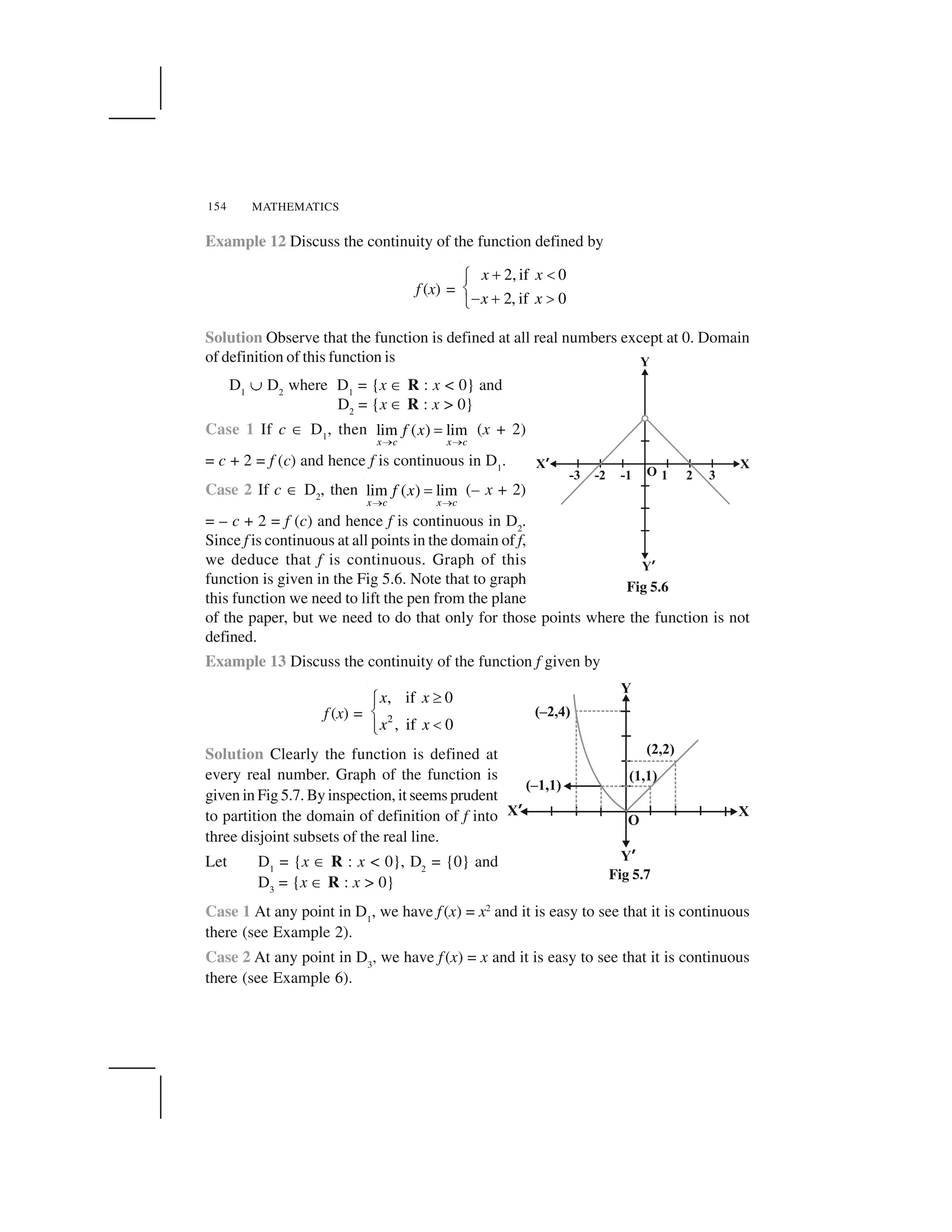
![CONTINUITY AND DIFFERENTIABILITY 155
Case 3 Now we analyse the function at x = 0. The value of the function at 0 is f(0) = 0.
The left hand limit of f at 0 is
–
2 2
0 0
lim ( ) lim 0 0
x x
f x x
✁ ✁
✂ ✂ ✂
The right hand limit of f at 0 is
0 0
lim ( ) lim 0
x x
f x x✄ ✄
☎ ☎
✆ ✆
Thus
0
lim ( ) 0
x
f x
☎
✆ = f (0) and hence f is continuous at 0. This means that f is
continuous at every point in its domain and hence, f is a continuous function.
Example 14 Show that every polynomial function is continuous.
Solution Recall that a function p is a polynomial function if it is defined by
p(x) = a0
+ a1
x + ... + an
xn
for some natural number n, an
✝ 0 and ai
✞ R. Clearly this
function is defined for every real number. For a fixed real number c, we have
lim ( ) ( )
x c
p x p c
✟
✠
By definition, p is continuous at c. Since c is any real number, p is continuous at
every real number and hence p is a continuous function.
Example 15 Find all the points of discontinuity of the greatest integer function defined
by f (x) = [x], where [x] denotes the greatest integer less than or equal to x.
Solution First observe that f is defined for all real numbers. Graph of the function is
given in Fig 5.8. From the graph it looks like that f is discontinuous at every integral
point. Below we explore, if this is true.
Fig 5.8](https://image.slidesharecdn.com/ncert-class-12-mathematics-part-1-161112165946/75/Ncert-class-12-mathematics-part-1-158-2048.jpg)
![MATHEMATICS156
Case 1 Let c be a real number which is not equal to any integer. It is evident from the
graph that for all real numbers close to c the value of the function is equal to [c]; i.e.,
lim ( ) lim [ ] [ ]
x c x c
f x x c
✁ ✁ .Also f (c) = [c] and hence the function is continuous at all real
numbers not equal to integers.
Case 2 Let c be an integer. Then we can find a sufficiently small real number
r > 0 such that [c – r] = c – 1 whereas [c + r] = c.
This, in terms of limits mean that
lim
x c✂
f (x) = c – 1, lim
x c✄☎ f (x) = c
Since these limits cannot be equal to each other for any c, the function is
discontinuous at every integral point.
5.2.1 Algebra of continuous functions
In the previous class, after having understood the concept of limits, we learnt some
algebra of limits.Analogously, now we will study some algebra of continuous functions.
Since continuity of a function at a point is entirely dictated by the limit of the function at
that point, it is reasonable to expect results analogous to the case of limits.
Theorem 1 Suppose f and g be two real functions continuous at a real number c.
Then
(1) f + g is continuous at x = c.
(2) f – g is continuous at x = c.
(3) f . g is continuous at x = c.
(4)
f
g
✆ ✝
✞ ✟
✠ ✡
is continuous at x = c, (provided g (c) ☛ 0).
Proof We are investigating continuity of (f + g) at x = c. Clearly it is defined at
x = c. We have
lim( )( )
x c
f g x
☞ = lim[ ( ) ( )]
x c
f x g x
☞ (by definition of f + g)
= lim ( ) lim ( )
x c x c
f x g x
☞ (by the theorem on limits)
= f (c) + g(c) (as f and g are continuous)
= (f + g) (c) (by definition of f + g)
Hence, f + g is continuous at x = c.
Proofs for the remaining parts are similar and left as an exercise to the reader.](https://image.slidesharecdn.com/ncert-class-12-mathematics-part-1-161112165946/75/Ncert-class-12-mathematics-part-1-159-2048.jpg)
![CONTINUITY AND DIFFERENTIABILITY 157
Remarks
(i) As a special case of (3) above, if f is a constant function, i.e., f (x) = ✝ for some
real number ✝, then the function (✝ . g) defined by (✝ . g) (x) = ✝ . g(x) is also
continuous. In particular if ✝ = – 1, the continuity of f implies continuity of – f.
(ii) As a special case of (4) above, if f is the constant function f (x) = ✝, then the
function
g
defined by ( )
( )
x
g g x
✁ ✁
✂ is also continuous wherever g(x) ✄ 0. In
particular, the continuity of g implies continuity of
1
g
.
The above theorem can be exploited to generate many continuous functions. They
also aid in deciding if certain functions are continuous or not. The following examples
illustrate this:
Example 16 Prove that every rational function is continuous.
Solution Recall that every rational function f is given by
( )
( ) , ( ) 0
( )
p x
f x q x
q x
☎ ✆
where p and q are polynomial functions. The domain of f is all real numbers except
points at which q is zero. Since polynomial functions are continuous (Example 14), f is
continuous by (4) of Theorem 1.
Example 17 Discuss the continuity of sine function.
Solution To see this we use the following facts
0
lim sin 0
x
x
✞
✟
We have not proved it, but is intuitively clear from the graph of sin x near 0.
Now, observe that f (x) = sin x is defined for every real number. Let c be a real
number. Put x = c + h. If x ✠ c we know that h ✠ 0. Therefore
lim ( )
x c
f x
✡ = lim sin
x c
x
✡
= 0
lim sin( )
h
c h
✞
☛
= 0
lim [sin cos cos sin ]
h
c h c h
✞
☛
= 0 0
lim [sin cos ] lim [cos sin ]
h h
c h c h
✞ ✞
☛
= sin c + 0 = sin c = f (c)
Thus lim
x c✡
f (x) = f (c) and hence f is a continuous function.](https://image.slidesharecdn.com/ncert-class-12-mathematics-part-1-161112165946/75/Ncert-class-12-mathematics-part-1-160-2048.jpg)
![MATHEMATICS160
Discuss the continuity of the function f, where f is defined by
14.
3, if 0 1
( ) 4, if 1 3
5, if 3 10
x
f x x
x
✁
✂
✄ ☎ ☎✆
✂ ✝
15.
2 , if 0
( ) 0, if 0 1
4 , if >1
x x
f x x
x x
✞✟
✠
✡ ☛ ☛☞
✠
✌
16.
2, if 1
( ) 2 , if 1 1
2, if 1
x
f x x x
x
✍ ✍✁
✂
✄ ✍ ☎ ✆
✂ ✎✝
17. Find the relationship between a and b so that the function f defined by
1, if 3
( )
3, if 3
ax x
f x
bx x
✏ ✑✒
✓ ✔
✏ ✕✖
is continuous at x = 3.
18. For what value of ✗ is the function defined by
2
( 2 ), if 0
( )
4 1, if 0
x x x
f x
x x
✘✙ ✚ ✛✜
✢ ✣
✤ ✥✜✦
continuous at x = 0? What about continuity at x = 1?
19. Show that the function defined by g (x) = x – [x] is discontinuous at all integral
points. Here [x] denotes the greatest integer less than or equal to x.
20. Is the function defined by f(x) = x2
– sin x + 5 continuous at x = ✧?
21. Discuss the continuity of the following functions:
(a) f (x) = sin x + cos x (b) f(x) = sin x – cos x
(c) f (x) = sin x . cos x
22. Discuss the continuity of the cosine, cosecant, secant and cotangent functions.
23. Find all points of discontinuity of f, where
sin
, if 0
( )
1, if 0
x
x
f x x
x x
★
✩✪
✫ ✬
✪ ✭ ✮✯
24. Determine if f defined by
2 1
sin , if 0
( )
0, if 0
x x
f x x
x
★
✰✪
✫ ✬
✪ ✫✯
is a continuous function?](https://image.slidesharecdn.com/ncert-class-12-mathematics-part-1-161112165946/75/Ncert-class-12-mathematics-part-1-163-2048.jpg)
![MATHEMATICS162
f (x) xn
sin x cos x tan x
f ✠(x) nxn – 1
cos x – sin x sec2
x
provided this limit exists. Derivative of f at c is denoted by f ✠(c) or ( ( )) |c
d
f x
dx
. The
function defined by
0
( ) ( )
( ) lim
h
f x h f x
f x
h
✁ ✂✄ ☎
wherever the limit exists is defined to be the derivative of f. The derivative of f is
denoted by f ✠(x) or ( ( ))
d
f x
dx
or if y = f (x) by
dy
dx
or y✠. The process of finding
derivative of a function is called differentiation. We also use the phrase differentiate
f (x) with respect to x to mean find f ✠(x).
The following rules were established as a part of algebra of derivatives:
(1) (u ± v)✠ = u✠ ± v✠
(2) (uv)✠ = u✠v + uv✠ (Leibnitz or product rule)
(3)
2
u u v uv
v v
✆ ✆ ✝ ✆✞ ✟ ✡☛ ☞✌ ✍
, wherever v ✎ 0 (Quotient rule).
The following table gives a list of derivatives of certain standard functions:
Table 5.3
Whenever we defined derivative, we had put a caution provided the limit exists.
Now the natural question is; what if it doesn’t? The question is quite pertinent and so is
its answer. If
0
( ) ( )
lim
h
f c h f c
h
✁ ✂ does not exist, we say that f is not differentiable at c.
In other words, we say that a function f is differentiable at a point c in its domain if both
–
0
( ) ( )
lim
h
f c h f c
h
✁ ✂ and
0
( ) ( )
lim
h
f c h f c
h✏
✁ ✂ are finite and equal.A function is said
to be differentiable in an interval [a, b] if it is differentiable at every point of [a, b].As
in case of continuity, at the end points a and b, we take the right hand limit and left hand
limit, which are nothing but left hand derivative and right hand derivative of the function
at a and b respectively. Similarly, a function is said to be differentiable in an interval
(a, b) if it is differentiable at every point of (a, b).](https://image.slidesharecdn.com/ncert-class-12-mathematics-part-1-161112165946/75/Ncert-class-12-mathematics-part-1-165-2048.jpg)
![CONTINUITY AND DIFFERENTIABILITY 163
Theorem 3 If a function f is differentiable at a point c, then it is also continuous at that
point.
Proof Since f is differentiable at c, we have
( ) ( )
lim ( )
x c
f x f c
f c
x c
✁
✂ ✄
✁
But for x ☎ c, we have
f (x) – f (c) =
( ) ( )
. ( )
f x f c
x c
x c
✁
✁
✁
Therefore lim[ ( ) ( )]
x c
f x f c
✆ ✝ =
( ) ( )
lim . ( )
x c
f x f c
x c
x c✞
✟✠ ✡✟☛ ☞✟✌ ✍
or lim [ ( )] lim [ ( )]
x c x c
f x f c
✆ ✆✝ =
( ) ( )
lim .lim[( )]
x c x c
f x f c
x c
x c✎ ✎
✏✑ ✒ ✏✓ ✔✏✕ ✖
= f✗(c) . 0 = 0
or lim ( )
x c
f x
✘ = f (c)
Hence f is continuous at x = c.
Corollary 1 Every differentiable function is continuous.
We remark that the converse of the above statement is not true. Indeed we have
seen that the function defined by f (x) = |x| is a continuous function. Consider the left
handlimit
–
0
(0 ) (0)
lim 1
h
f h f h
h h
✙ ✁ ✁
✂ ✂ ✁
The right hand limit
0
(0 ) (0)
lim 1
h
f h f h
h h✚
✙ ✁
✂ ✂
Since the above left and right hand limits at 0 are not equal,
0
(0 ) (0)
lim
h
f h f
h
✙ ✁
does not exist and hence f is not differentiable at 0. Thus f is not a differentiable
function.
5.3.1 Derivatives of composite functions
To study derivative of composite functions, we start with an illustrative example. Say,
we want to find the derivative of f, where
f (x) = (2x + 1)3](https://image.slidesharecdn.com/ncert-class-12-mathematics-part-1-161112165946/75/Ncert-class-12-mathematics-part-1-166-2048.jpg)
![MATHEMATICS166
Alternatively, we can proceed as follows:
y = sin (cos x2
)
Therefore
dy d
dx dx
sin (cos x2
) = cos (cos x2
)
d
dx
(cos x2
)
= cos (cos x2
) (– sin x2
)
d
dx
(x2
)
= – sin x2
cos (cos x2
) (2x)
= – 2x sin x2
cos (cos x2
)
EXERCISE 5.2
Differentiate the functions with respect to x in Exercises 1 to 8.
1. sin (x2
+ 5) 2. cos (sin x) 3. sin (ax + b)
4. sec (tan ( x )) 5.
sin ( )
cos ( )
ax b
cx d
✁
✁ 6. cos x3
. sin2
(x5
)
7. ✂ ✄2
2 cot x 8. ☎ ✆cos x
9. Prove that the function f given by
f (x) = |x – 1|, x ✝ R
is not differentiable at x = 1.
10. Prove that the greatest integer function defined by
f (x) = [x], 0 < x < 3
is not differentiable at x = 1 and x = 2.
5.3.2 Derivatives of implicit functions
Until now we have been differentiating various functions given in the form y = f (x).
But it is not necessary that functions are always expressed in this form. For example,
consider one of the following relationships between x and y:
x – y – ✟ = 0
x + sin xy – y = 0
In the first case, we can solve for y and rewrite the relationship as y = x – ✟. In
the second case, it does not seem that there is an easy way to solve for y. Nevertheless,
there is no doubt about the dependence of y on x in either of the cases. When a
relationship between x and y is expressed in a way that it is easy to solve for y and
write y = f(x), we say that y is given as an explicit function of x. In the latter case it](https://image.slidesharecdn.com/ncert-class-12-mathematics-part-1-161112165946/75/Ncert-class-12-mathematics-part-1-169-2048.jpg)
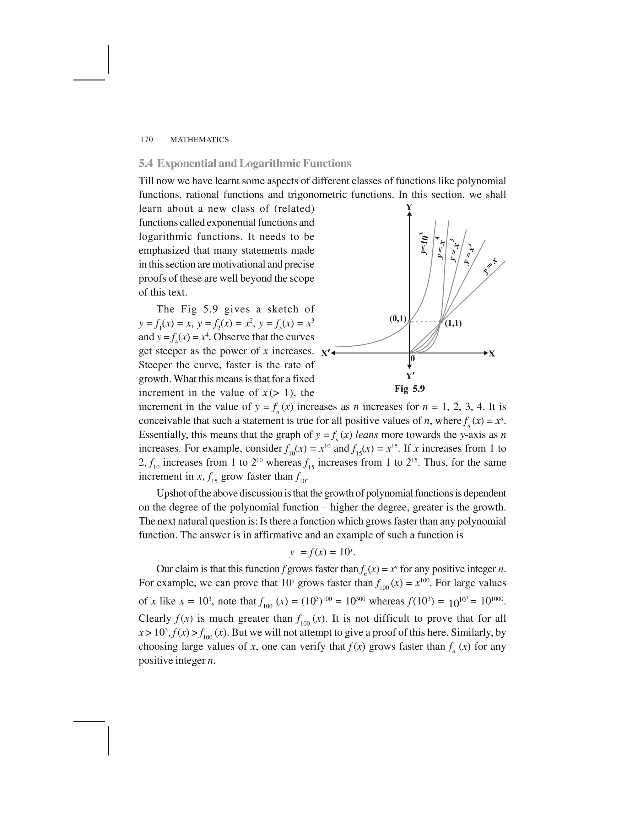
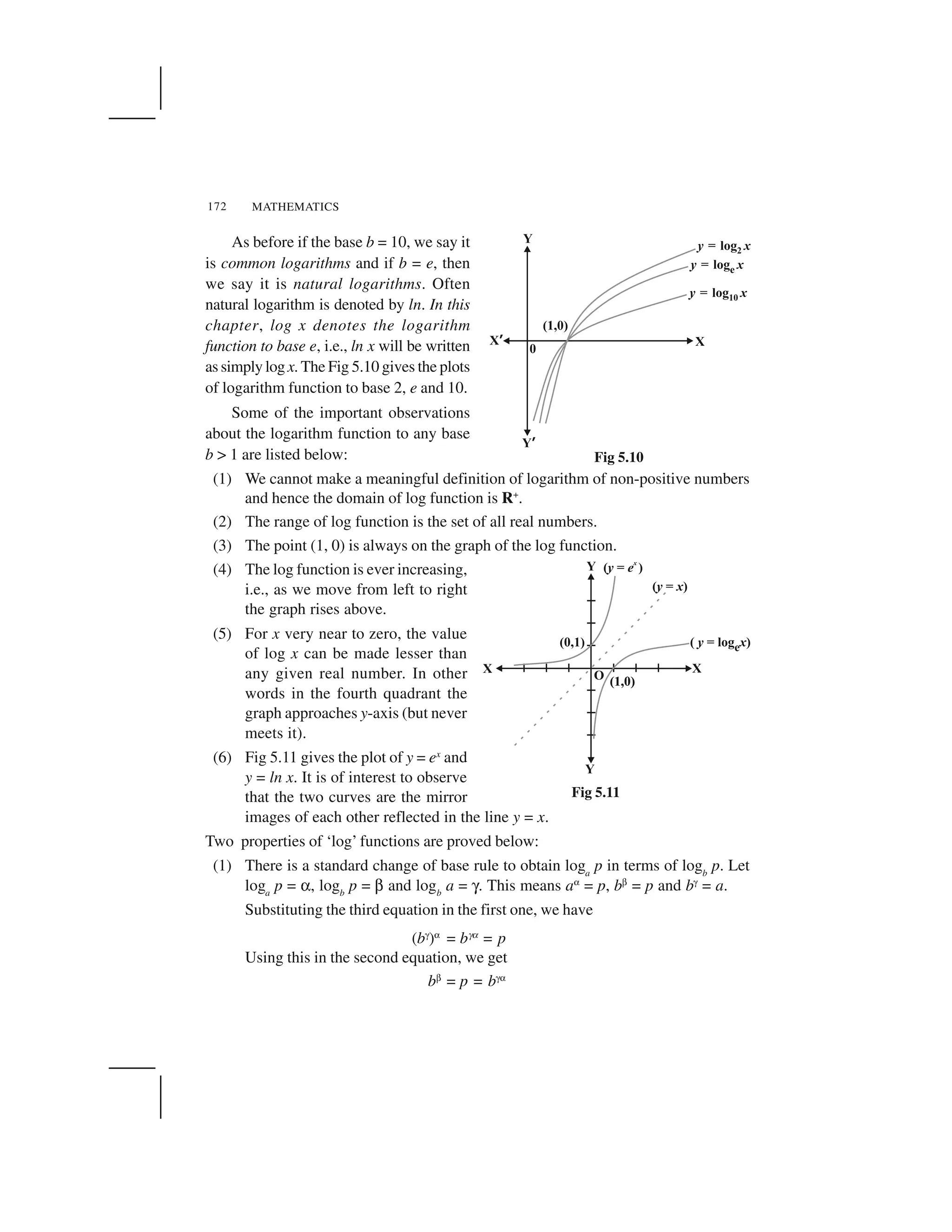
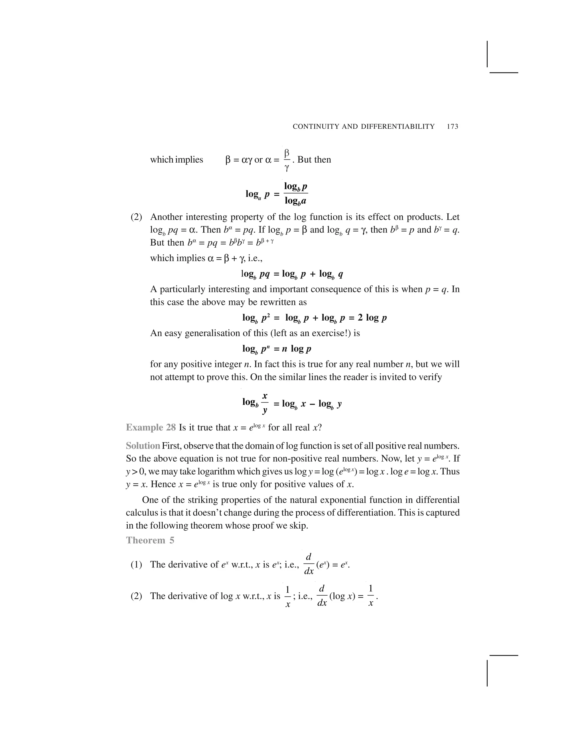
![MATHEMATICS174
Example 29 Differentiate the following w.r.t. x:
(i) e–x
(ii) sin (log x), x > 0 (iii) cos–1
(ex
) (iv) ecos x
Solution
(i) Let y = e– x
. Using chain rule, we have
dy
dx
=
x d
e
dx
✁ (– x) = – e– x
(ii) Let y = sin (log x). Using chain rule, we have
dy
dx
=
cos (log )
cos (log ) (log )
d x
x x
dx x
✁ ✂
(iii) Let y = cos–1
(ex
). Using chain rule, we have
dy
dx
= 2 2
1
( )
1 ( ) 1
x
x
x x
d e
e
dxe e
✄ ✄
☎ ✆
✄ ✄
(iv) Let y = ecos x
. Using chain rule, we have
dy
dx
= cos cos
( sin ) (sin )x x
e x x e✝ ✞ ✟ ✞
EXERCISE 5.4
Differentiate the following w.r.t. x:
1.
sin
x
e
x
2.
1
sin x
e
✠
3.
3
x
e
4. sin (tan–1
e–x
) 5. log (cos ex
) 6.
2 5
...x x x
e e e✡ ✡ ✡
7. , 0x
e x ☛ 8. log (log x), x > 1 9.
cos
, 0
log
x
x
x
☞
10. cos (log x + ex
), x > 0
5.5. Logarithmic Differentiation
In this section, we will learn to differentiate certain special class of functions given in
the form
y = f (x) = [u(x)]v (x)
By taking logarithm (to base e) the above may be rewritten as
log y = v(x) log [u(x)]](https://image.slidesharecdn.com/ncert-class-12-mathematics-part-1-161112165946/75/Ncert-class-12-mathematics-part-1-177-2048.jpg)
![CONTINUITY AND DIFFERENTIABILITY 175
Using chain rule we may differentiate this to get
1 1
( )
( )
dy
v x
y dx u x
✁ . u✠(x) + v✠(x) . log [u(x)]
which implies that
✂ ✄
( )
( ) ( ) log ( )
( )
dy v x
y u x v x u x
dx u x
☎ ✆
✝ ✞ ✟ ✡ ✟ ✞
☛ ☞
✌ ✍
The main point to be noted in this method is that f (x) and u(x) must always be
positive as otherwise their logarithms are not defined. This process of differentiation is
known as logarithms differentiation and is illustrated by the following examples:
Example 30 Differentiate
2
2
( 3) ( 4)
3 4 5
x x
x x
✎ ✏
✏ ✏
w.r.t. x.
Solution Let
2
2
( 3) ( 4)
(3 4 5)
x x
y
x x
✑ ✒
✓
✒ ✒
Taking logarithm on both sides, we have
log y =
1
2
[log (x – 3) + log (x2
+ 4) – log (3x2
+ 4x + 5)]
Now, differentiating both sides w.r.t. x, we get
1 dy
y dx
✔ = 2 2
1 1 2 6 4
2 ( 3) 4 3 4 5
x x
x x x x
✡☎ ✆
✡ ✕
☛ ☞
✕ ✡ ✡ ✡✌ ✍
or
dy
dx
= 2 2
1 2 6 4
2 ( 3) 4 3 4 5
y x x
x x x x
✖✗ ✘
✖ ✙
✚ ✛
✙ ✖ ✖ ✖✜ ✢
=
2
2 2 2
1 ( 3)( 4) 1 2 6 4
2 ( 3)3 4 5 4 3 4 5
x x x x
xx x x x x
✣ ✤ ✤✥ ✦
✤ ✣
✧ ★
✣✤ ✤ ✤ ✤ ✤✩ ✪
Example 31 Differentiate ax
w.r.t. x, where a is a positive constant.
Solution Let y = ax
. Then
log y = x log a
Differentiating both sides w.r.t. x, we have
1 dy
y dx = log a](https://image.slidesharecdn.com/ncert-class-12-mathematics-part-1-161112165946/75/Ncert-class-12-mathematics-part-1-178-2048.jpg)
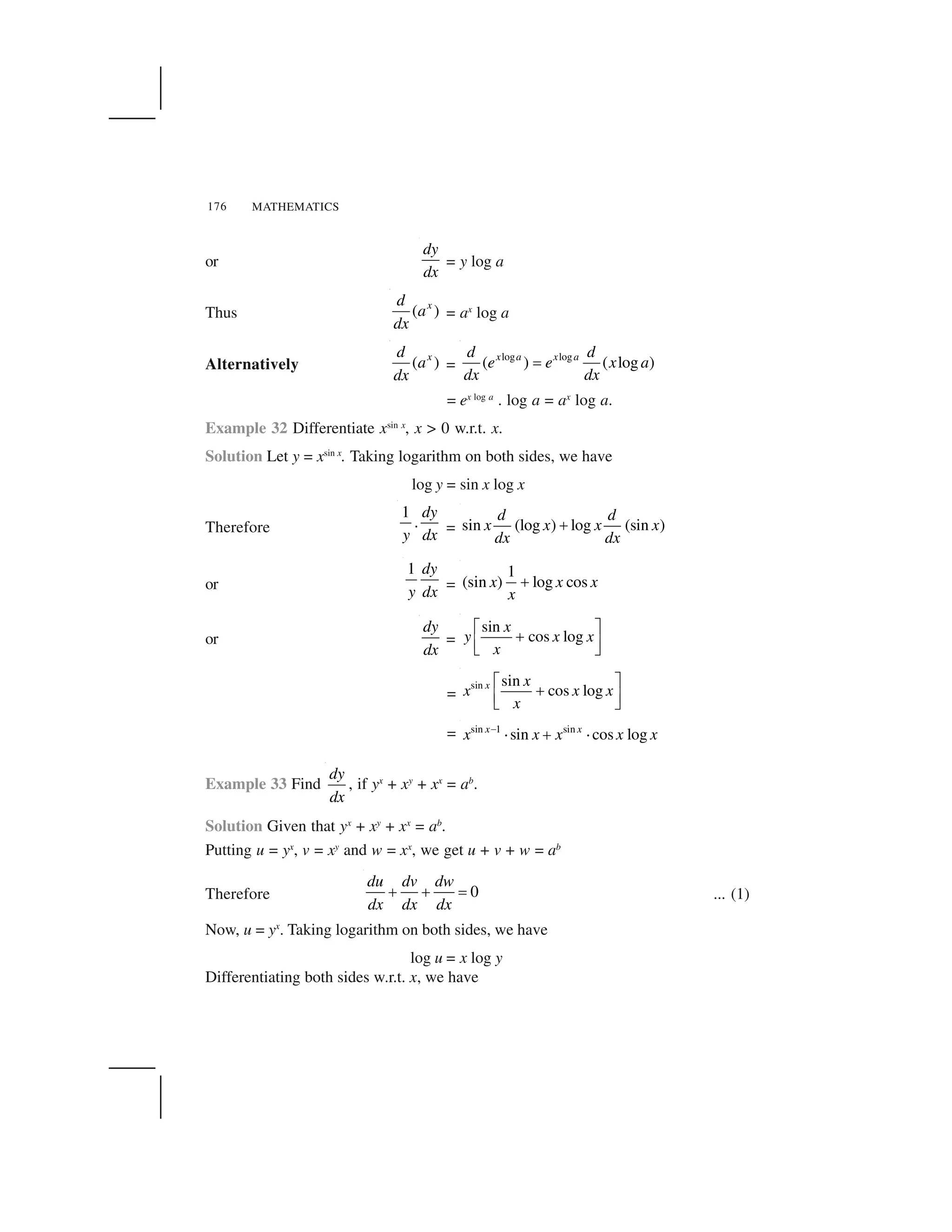
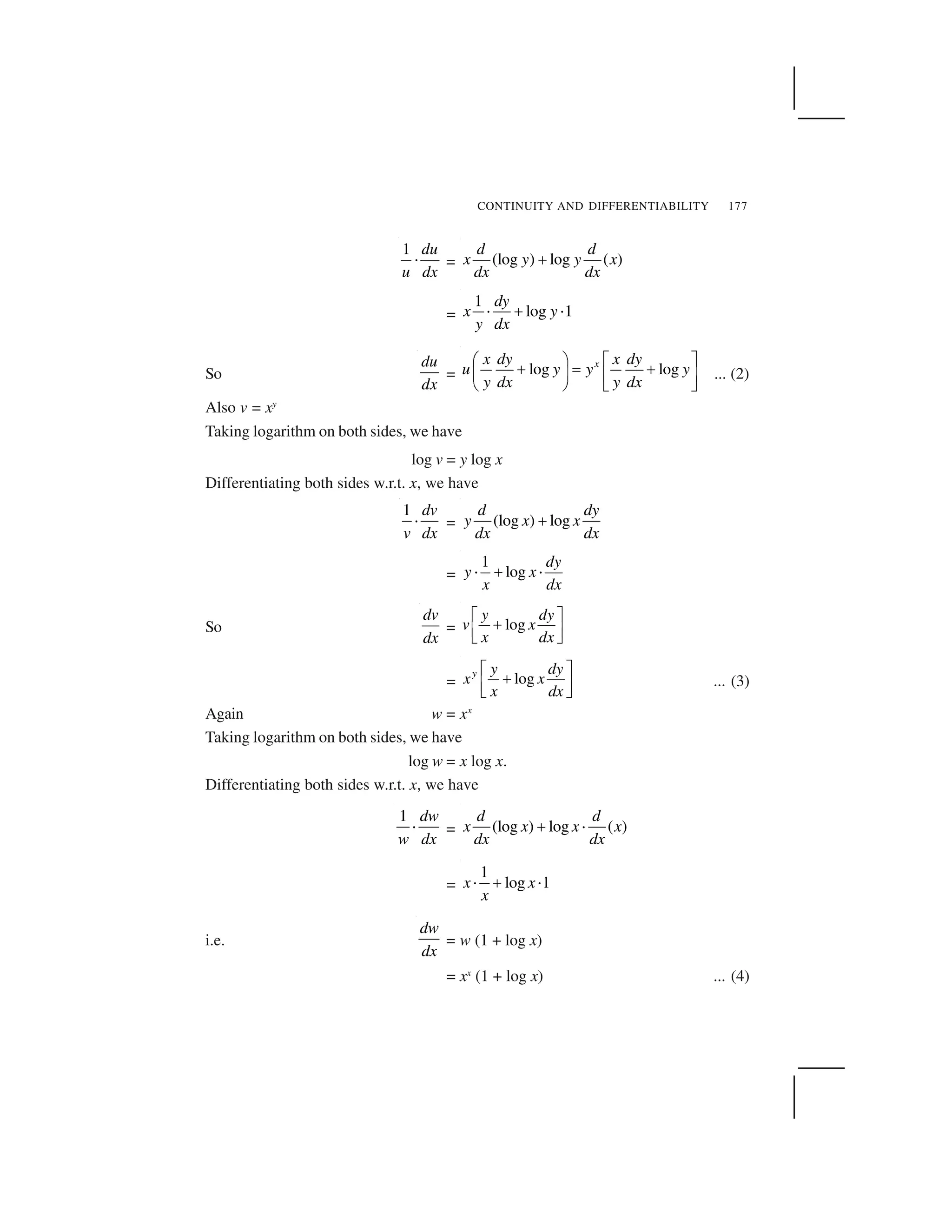
![MATHEMATICS178
From (1), (2), (3), (4), we have
log logx yx dy y dy
y y x x
y dx x dx
✁ ✁
✂ ✂ ✂✄ ☎✄ ☎
✆ ✝✆ ✝
+ xx
(1 + log x) = 0
or (x . yx –1
+ xy
. log x)
dy
dx
= – xx
(1 + log x) – y . xy–1
– yx
log y
Therefore
dy
dx
=
1
1
[ log . (1 log )]
. log
x y x
x y
y y y x x x
x y x x
✞
✞
✟ ✠ ✠ ✠
✠
EXERCISE 5.5
Differentiate the functions given in Exercises 1 to 11 w.r.t. x.
1. cos x . cos 2x . cos 3x 2.
( 1) ( 2)
( 3) ( 4) ( 5)
x x
x x x
✡ ✡
✡ ✡ ✡
3. (log x)cos x
4. xx
– 2sin x
5. (x + 3)2
. (x + 4)3
. (x + 5)4
6.
1
11
x
x
x x
x
☛ ☞✌✍ ✎
✏ ✑✒ ✓
✠ ✠✔ ✕
✖ ✗
7. (log x)x
+ xlog x
8. (sin x)x
+ sin–1
x
9. xsin x
+ (sin x)cos x
10.
2
cos
2
1
1
x x x
x
x
✘
✘
✙
11. (x cos x)x
+
1
( sin )xx x
Find
dy
dx
of the functions given in Exercises 12 to 15.
12. xy
+ yx
= 1 13. yx
= xy
14. (cos x)y
= (cos y)x
15. xy = e(x – y)
16. Find the derivative of the function given by f(x) = (1 + x) (1 + x2
) (1 + x4
) (1 + x8
)
and hence find f ✚(1).
17. Differentiate (x2
– 5x + 8) (x3
+ 7x + 9) in three ways mentioned below:
(i) by using product rule
(ii) by expanding the product to obtain a single polynomial.
(iii) by logarithmic differentiation.
Do they all give the same answer?](https://image.slidesharecdn.com/ncert-class-12-mathematics-part-1-161112165946/75/Ncert-class-12-mathematics-part-1-181-2048.jpg)
![CONTINUITY AND DIFFERENTIABILITY 179
18. If u, v and w are functions of x, then show that
d
dx
(u. v. w) =
du
dx
v. w + u .
dv
dx
. w + u . v
dw
dx
in two ways - first by repeated application of product rule, second by logarithmic
differentiation.
5.6 Derivatives of Functions in Parametric Forms
Sometimes the relation between two variables is neither explicit nor implicit, but some
link of a third variable with each of the two variables, separately, establishes a relation
between the first two variables. In such a situation, we say that the relation between
them is expressed via a third variable. The third variable is called the parameter. More
precisely, a relation expressed between two variables x and y in the form
x = f (t), y = g (t) is said to be parametric form with t as a parameter.
In order to find derivative of function in such form, we have by chain rule.
dy
dt
=
dy dx
dx dt
or
dy
dx
= whenever 0
dy
dxdt
dx dt
dt
✁ ✂
✄☎ ✆
✝ ✞
Thus
dy
dx
=
( )
as ( ) and ( )
( )
g t dy dx
g t f t
f t dt dt
✟ ✠ ✡
☛ ✟ ☛ ✟☞ ✌
✟ ✍ ✎
[provided f ✏(t) ✑ 0]
Example 34 Find
dy
dx
, if x = a cos ✒, y = a sin ✒.
Solution Given that
x = a cos ✒, y = a sin ✒
Therefore
dx
d✓
= – a sin ✒,
dy
d✓
= a cos ✒
Hence
dy
dx
=
cos
cot
sin
dy
ad
dx a
d
✔✔
✕ ✕ ✖ ✔
✖ ✔
✔](https://image.slidesharecdn.com/ncert-class-12-mathematics-part-1-161112165946/75/Ncert-class-12-mathematics-part-1-182-2048.jpg)
![MATHEMATICS184
12. If y = cos–1
x, Find
2
2
d y
dx
in terms of y alone.
13. If y = 3 cos (log x) + 4 sin (log x), show that x2
y2
+ xy1
+ y = 0
14. If y = Aemx
+ Benx
, show that
2
2
( ) 0
d y dy
m n mny
dxdx
✁ ✁ ✂
15. If y = 500e7x
+ 600e–7x
, show that
2
2
49
d y
y
dx
✄
16. If ey
(x + 1) = 1, show that
22
2
d y dy
dxdx
☎ ✆✝ ✞ ✟
✠ ✡
17. If y = (tan–1
x)2
, show that (x2
+ 1)2
y2
+ 2x (x2
+ 1) y1
= 2
5.8 Mean Value Theorem
In this section, we will state two fundamental results in Calculus without proof. We
shall also learn the geometric interpretation of these theorems.
Theorem 6 (Rolle’s Theorem) Let f : [a, b] ☛ R be continuous on [a, b] and
differentiable on (a, b), such that f(a) = f(b), where a and b are some real numbers.
Then there exists some c in (a, b) such that f☞(c) = 0.
In Fig 5.12 and 5.13, graphs of a few typical differentiable functions satisfying the
hypothesis of Rolle’s theorem are given.
Fig 5.12 Fig 5.13
Observe what happens to the slope of the tangent to the curve at various points
between a and b. In each of the graphs, the slope becomes zero at least at one point.
That is precisely the claim of the Rolle’s theorem as the slope of the tangent at any
point on the graph of y = f (x) is nothing but the derivative of f (x) at that point.](https://image.slidesharecdn.com/ncert-class-12-mathematics-part-1-161112165946/75/Ncert-class-12-mathematics-part-1-187-2048.jpg)
![CONTINUITY AND DIFFERENTIABILITY 185
Theorem 7 (Mean Value Theorem) Let f : [a, b] ✞ R be a continuous function on
[a, b] and differentiable on (a, b). Then there exists some c in (a, b) such that
( ) ( )
( )
f b f a
f c
b a
✁ ✂
Observe that the Mean Value Theorem (MVT) is an extension of Rolle’s theorem.
Let us now understand a geometric interpretation of the MVT. The graph of a function
y = f(x) is given in the Fig 5.14. We have already interpreted f ✠(c) as the slope of the
tangent to the curve y = f(x) at (c, f(c)). From the Fig 5.14 it is clear that
( ) ( )f b f a
b a
is the slope of the secant drawn between (a, f(a)) and (b, f(b)). The MVT states that
there is a point c in (a, b) such that the slope of the tangent at (c, f(c)) is same as the
slope of the secant between (a, f(a)) and (b, f(b)). In other words, there is a point c in
(a, b) such that the tangent at (c, f(c)) is parallel to the secant between (a, f(a)) and
(b, f(b)).
Fig 5.14
Example 42 Verify Rolle’s theorem for the function y = x2
+ 2, a = – 2 and b = 2.
Solution The function y = x2
+ 2 is continuous in [– 2, 2] and differentiable in (– 2, 2).
Also f(– 2) = f( 2) = 6 and hence the value of f(x) at – 2 and 2 coincide. Rolle’s
theorem states that there is a point c ✆ (– 2, 2), where f✄(c) = 0. Since f✄(x) = 2x, we
get c = 0. Thus at c = 0, we have f✄(c) = 0 and c = 0 ✆ (– 2, 2).
Example 43 Verify Mean Value Theorem for the function f(x) = x2
in the interval [2, 4].
Solution The function f (x) = x2
is continuous in [2, 4] and differentiable in (2, 4) as its
derivative f✄(x) = 2xis defined in (2, 4).](https://image.slidesharecdn.com/ncert-class-12-mathematics-part-1-161112165946/75/Ncert-class-12-mathematics-part-1-188-2048.jpg)
![MATHEMATICS186
Now, f(2) = 4 and f (4) = 16. Hence
( ) ( ) 16 4
6
4 2
f b f a
b a
✁ ✁
MVT states that there is a point c ✆ (2, 4) such that f✠(c) = 6. But f✠(x) = 2x which
implies c = 3. Thus at c = 3 ✆ (2, 4), we have f✠(c) = 6.
EXERCISE 5.8
1. Verify Rolle’s theorem for the function f(x) = x2
+ 2x – 8, x ✆ [– 4, 2].
2. Examine if Rolle’s theorem is applicable to any of the following functions. Can
you say some thing about the converse of Rolle’s theorem from these example?
(i) f(x) = [x] for x ✆ [5, 9] (ii) f(x) = [x] for x ✆ [– 2, 2]
(iii) f(x) = x2
– 1 for x ✆ [1, 2]
3. If f : [– 5, 5] ✞ R is a differentiable function and if f✂(x) does not vanish
anywhere, then prove that f(– 5) ✄ f(5).
4. Verify Mean Value Theorem, if f(x) = x2
– 4x – 3 in the interval [a, b], where
a = 1 and b = 4.
5. Verify Mean Value Theorem, if f(x) = x3
– 5x2
– 3x in the interval [a, b], where
a = 1 and b = 3. Find all c ✆ (1, 3) for which f✂(c) = 0.
6. Examine the applicability of MeanValue Theorem for all three functions given in
the above exercise 2.
Miscellaneous Examples
Example 44 Differentiate w.r.t. x, the following function:
(i)
2
1
3 2
2 4
x
x
☎ ☎
☎
(ii)
2
sec –1
3cosx
e x✝ (iii) log7
(log x)
Solution
(i) Let y = 2
1
3 2
2 4
x
x
☎ ☎
☎
=
1 1
22 2(3 2) (2 4)x x
✟
✡ ✡ ✡
Note that this function is defined at all real numbers
2
3
x ☛ . Therefore
dy
dx
=
1 1
1 1
2 22 2
1 1
(3 2) (3 2) (2 4) (2 4)
2 2
d d
x x x x
dx dx
☞ ☞ ☞✌ ✍
☎ ✎ ☎ ☎ ✏ ☎ ✎ ☎✑ ✒
✓ ✔](https://image.slidesharecdn.com/ncert-class-12-mathematics-part-1-161112165946/75/Ncert-class-12-mathematics-part-1-189-2048.jpg)
![CONTINUITY AND DIFFERENTIABILITY 187
=
1 3
22 2
1 1
(3 2) (3) (2 4) 4
2 2
x x x
✁ ✂
✄ ☎ ✆ ✄ ☎✝ ✞
✟ ✠
=
✡ ☛
3
2 2
3 2
2 3 2
2 4
x
x
x
☞
✌
✌
This is defined for all real numbers
2
3
x ✍ ✎ .
(ii) Let
2
sec 1
3cosx
y e x✏
✑ ✒
This is defined at every real number in ✓ ✔[ 1,1] 0✕ ✕ . Therefore
dy
dx
=
2
sec 2
2
1
(sec ) 3
1
x d
e x
dx x
✖ ✗
✘ ✙ ✚
✛ ✜
✢ ✣✚
=
2
sec
2
1
2sec (sec ) 3
1
x d
e x x
dx x
✖ ✗ ✖ ✗
✘ ✙ ✚✛ ✜ ✛ ✜✢ ✣ ✢ ✣✚
=
2
sec
2
1
2sec (sec tan ) 3
1
x
x x x e
x
✖ ✗
✙ ✚✛ ✜
✚✢ ✣
=
2
2 sec
2
1
2sec tan 3
1
x
x x e
x
✤ ✥
✦ ✧★ ✩
✧✪ ✫
Observe that the derivative of the given function is valid only in ✓ ✔[ 1,1] 0✕ ✕ as
the derivative of cos–1
x exists only in (– 1, 1) and the function itself is not
defined at 0.
(iii) Let y = log7
(log x) =
log (log )
log7
x
(by change of base formula).
The function is defined for all real numbers x > 1. Therefore
dy
dx
=
1
(log (log ))
log7
d
x
dx
=
1 1
(log )
log7 log
d
x
x dx
✬
=
1
log7 logx x](https://image.slidesharecdn.com/ncert-class-12-mathematics-part-1-161112165946/75/Ncert-class-12-mathematics-part-1-190-2048.jpg)
![CONTINUITY AND DIFFERENTIABILITY 189
we need to find all x such that
1
2
1
1 4
x
x
✁
✂
, i.e., all x such that 2x + 1
✏ 1 + 4x
. We
may rewrite this as 2 ✏
1
2x
+ 2x
which is true for all x. Hence the function
is defined at every real number. By putting 2x
= tan ✍, this function may be
rewritten as
f(x) =
1
1 2
sin
1 4
x
x
✄
☎ ✆ ✝
✞ ✟
✠✡ ☛
=
☞ ✌
1
2
2 2
sin
1 2
x
x
✎ ✑ ✒✓
✔ ✕
✔ ✕✖✗ ✘
=
1
2
2tan
sin
1 tan
✙ ✚✛ ✜
✢ ✣
✤ ✚✥ ✦
= sin–1
[sin 2✍]
= 2✍ = 2 tan–1
(2x
)
Thus f✧(x) =
★ ✩
2
1
2 (2 )
1 2
x
x
d
dx
✪ ✪
✫
=
2
(2 )log2
1 4
x
x
✬
✭
=
1
2 log2
1 4
x
x
✮
✤
Example 46 Find f ✧(x) if f(x) = (sin x)sin x
for all 0 < x < ✯.
Solution The function y = (sin x)sin x
is defined for all positive real numbers. Taking
logarithms, we have
log y = log (sin x)sin x
= sin x log (sin x)
Then
1 dy
y dx
=
d
dx
(sin x log (sin x))
= cos x log (sin x) + sin x .
1
(sin )
sin
d
x
x dx
✰
= cos x log (sin x) + cos x
= (1 + log (sin x)) cos x](https://image.slidesharecdn.com/ncert-class-12-mathematics-part-1-161112165946/75/Ncert-class-12-mathematics-part-1-192-2048.jpg)
![CONTINUITY AND DIFFERENTIABILITY 193
Chain rule is rule to differentiate composites of functions. If f = v o u, t = u (x)
and if both
dt
dx
and
dv
dt
exist then
df dv dt
dx dt dx
✁ ✂
Following are some of the standard derivatives (in appropriate domains):
✄ ☎1
2
1
sin
1
d
x
dx x
✆ ✝
✞
✟ ✠1
2
1
cos
1
d
x
dx x
✆ ✝✞
✞
✡ ☛1
2
1
tan
1
d
x
dx x
☞ ✌ ✍
✡ ☛1
2
1
cot
1
d
x
dx x
☞ ✎✌ ✍
✏ ✑1
2
1
sec
1
d
x
dx x x
✒ ✓
✔
✕ ✖1
2
1
cosec
1
d
x
dx x x
✒ ✔✓
✔
✗ ✘x xd
e e
dx
✙ ✚ ✛ 1
log
d
x
dx x
✙
Logarithmic differentiation is a powerful technique to differentiate functions
of the form f (x) = [u (x)]v (x)
. Here both f (x) and u(x) need to be positive for
this technique to make sense.
Rolle’s Theorem: If f : [a, b] ✜R is continuous on [a, b] and differentiable
on (a, b) such that f (a) = f (b), then there exists some c in (a, b) such that
f ✢(c) = 0.
Mean Value Theorem: If f : [a, b] ✜ R is continuous on [a, b] and
differentiable on (a, b). Then there exists some c in (a, b) such that
( ) ( )
( )
f b f a
f c
b a
✣✤ ✁ ✣
—✥✥✥✥—](https://image.slidesharecdn.com/ncert-class-12-mathematics-part-1-161112165946/75/Ncert-class-12-mathematics-part-1-196-2048.jpg)
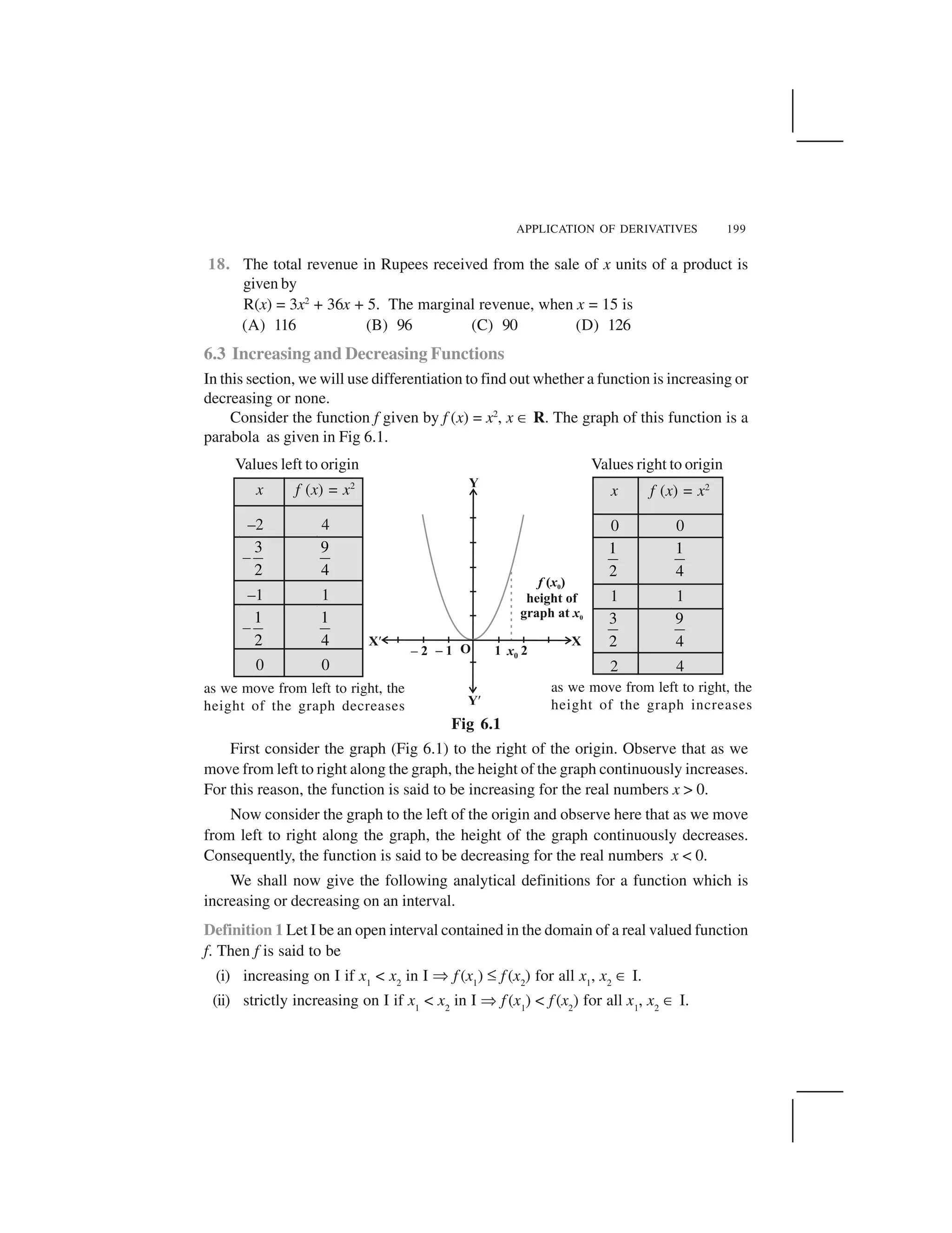
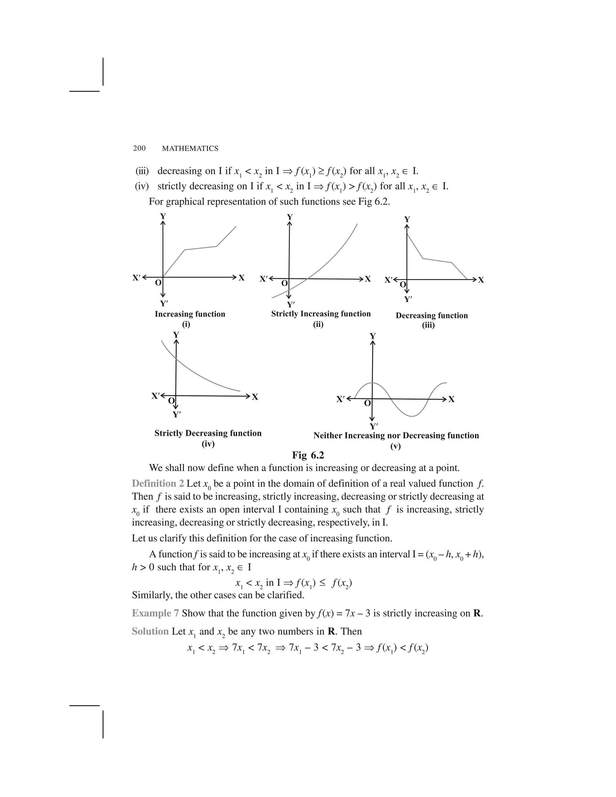
![APPLICATION OF DERIVATIVES 201
Thus, by Definition 1, it follows that f is strictly increasing on R.
We shall now give the first derivative test for increasing and decreasing functions.
The proof of this test requires the Mean Value Theorem studied in Chapter 5.
Theorem 1 Let f be continuous on [a, b] and differentiable on the open interval
(a,b). Then
(a) f is increasing in [a,b] if f ✂(x) > 0 for each x ☎ (a, b)
(b) f is decreasing in [a,b] if f ✂(x) < 0 for each x ☎ (a, b)
(c) f is a constant function in [a,b] if f ✂(x) = 0 for each x ☎ (a, b)
Proof (a) Let x1
, x2
☎ [a, b] be such that x1
< x2
.
Then, by Mean Value Theorem (Theorem 8 in Chapter 5), there exists a point c
between x1
and x2
such that
f(x2
) – f(x1
) = f ✂(c) (x2
– x1
)
i.e. f(x2
) – f(x1
) > 0 (as f ✂(c) > 0 (given))
i.e. f(x2
) > f (x1
)
Thus, we have
1 2 1 2 1 2( ) ( ), for all , [ , ]x x f x f x x x a b ✁ ✄
Hence, f is an increasing function in [a,b].
The proofs of part (b) and (c) are similar. It is left as an exercise to the reader.
Remarks
(i) f is strictly increasing in (a, b) if f ✂(x) > 0 for each x ☎ (a, b)
(ii) f is strictly decreasing in (a, b) if f ✂(x) < 0 for each x ☎ (a, b)
(iii) A function will be increasing (decreasing) in R if it is so in every interval of R.
Example 8 Show that the function f given by
f (x) = x3
– 3x2
+ 4x, x ☎ R
is strictly increasing on R.
Solution Note that
f ✂(x) = 3x2
– 6x + 4
= 3(x2
– 2x + 1) + 1
= 3(x – 1)2
+ 1 > 0, in every interval of R
Therefore, the function f is strictly increasing on R.](https://image.slidesharecdn.com/ncert-class-12-mathematics-part-1-161112165946/75/Ncert-class-12-mathematics-part-1-204-2048.jpg)
![MATHEMATICS202
Example 9 Prove that the function given by f (x) = cos x is
(a) strictly decreasing in (0, ✄)
(b) strictly increasing in (✄, 2✄), and
(c) neither increasing nor decreasing in (0, 2✄).
Solution Note that f ✂(x) = – sin x
(a) Since for each x ☎(0, ✄), sin x > 0, we have f ✂(x) < 0 and so f is strictly
decreasing in (0, ✄).
(b) Since for each x ☎(✄, 2✄), sin x < 0, we have f ✂(x) > 0 and so f is strictly
increasing in (✄, 2✄).
(c) Clearly by (a) and (b) above, f is neither increasing nor decreasing in (0, 2✄).
Note One may note that the function in Example 9 is neither strictly increasing in
[✄, 2✄] nor strictly decreasing in [0, ✄]. However, since the function is continuous at
the end points 0 and ✄, by Theorem 1, f is increasing in [✄, 2✄] and decreasing in [0,✄].
Example 10 Find the intervals in which the function f given by f(x) = x2
– 4x + 6 is
(a) strictly increasing (b) strictly decreasing
Solution We have
f (x) = x2
– 4x + 6
or f ✂(x) = 2x – 4
Therefore, f ✂(x) = 0 gives x = 2. Now the point x = 2 divides the real line into two
disjoint intervals namely, (– ✟, 2) and (2, ✟) (Fig 6.3). In the interval (– ✟, 2),
f ✂(x) = 2x – 4 < 0.
Therefore, f is strictly decreasing in this
interval. Also, in the interval (2, )✁ , ( ) 0f x ✆✝and so the function f is strictly increasing in this
interval.
Note Note that the given function is continuous at 2 which is the point joining
the two intervals. So, by Theorem 1, we conclude that the given function is decreasing
in (– ✟, 2] and increasing in [2, ✟).
Example 11 Find the intervals in which the function f given by f (x) = 4x3
– 6x2
– 72x + 30
is (a) strictly increasing (b) strictly decreasing.
Solution We have
f(x) = 4x3
– 6x2
– 72x + 30
Fig 6.3](https://image.slidesharecdn.com/ncert-class-12-mathematics-part-1-161112165946/75/Ncert-class-12-mathematics-part-1-205-2048.jpg)
![MATHEMATICS204
Therefore, f is strictly increasing in 0,
6
✁ ✂
✄☎✆ ✝
and strictly decreasing in ,
6 2
✞ ✞✟ ✠
✡ ☛
☞ ✌
.
Also, the given function is continuous at x = 0 and
6
x
✍
✎ . Therefore, by Theorem 1,
f is increasing on 0,
6
✏✑ ✒
✓ ✔✕ ✖
and decreasing on ,
6 2
✏ ✏✑ ✒
✓ ✔✕ ✖
.
Example 13 Find the intervals in which the function f given by
f (x) = sin x + cos x, 0 ✗ x ✗ 2✘
is strictly increasing or strictly decreasing.
Solution We have
f(x) = sin x + cos x,
or f ✙(x) = cos x – sin x
Now ( ) 0f x ✚✛ gives sin x = cos x which gives that
4
x
✍
✎ ,
5
4
✍
as 0 2x✜ ✜ ✢
The points
4
x
✣
✤ and
5
4
x
✣
✤ divide the interval [0, 2✘] into three disjoint intervals,
namely, 0,
4
✁ ✂
✄☎✆ ✝
,
5
,
4 4
✥ ✂
✦ ✄✧ ✝ and
5
,2
4
✏★ ✒
✏✩ ✔✪ ✖
.
Note that
5
( ) 0 if 0, ,2
4 4
f x x
✁ ✂ ✥ ✫✬ ✭ ✮ ✯ ✄ ✦☎ ✰✆ ✝ ✧ ✱
or f is strictly increasing in the intervals 0,
4
✁ ✂
✄☎✆ ✝
and
5
,2
4
✥ ✫ ✦ ✰✧ ✱
Also
5
( ) 0 if ,
4 4
f x x
✥ ✂
✲ ✮✬ ✦ ✄✧ ✝
or f is strictly decreasing in
5
,
4 4
✥ ✂
✦ ✄✧ ✝
Fig 6.6](https://image.slidesharecdn.com/ncert-class-12-mathematics-part-1-161112165946/75/Ncert-class-12-mathematics-part-1-207-2048.jpg)
![APPLICATION OF DERIVATIVES 205
Interval Sign of ( )f x Nature of function
0,
4
✁✂ ✄
☎✆
✝ ✞
> 0 f is strictly increasing
5
,
4 4
✟ ✟✠ ✡
☛ ☞
✌ ✍
< 0 f is strictly decreasing
5
,2
4
✁✎ ✏
✁
✑ ✒
✓ ✔
> 0 f is strictly increasing
EXERCISE 6.2
1. Show that the function given by f (x) = 3x + 17 is strictly increasing on R.
2. Show that the function given by f (x) = e2x
is strictly increasing on R.
3. Show that the function given by f (x) = sin x is
(a) strictly increasing in 0,
2
✟✠ ✡
☛ ☞
✌ ✍
(b) strictly decreasing in ,
2
✟✠ ✡
✟
☛ ☞
✌ ✍
(c) neither increasing nor decreasing in (0, ✕)
4. Find the intervals in which the function f given by f (x) = 2x2
– 3x is
(a) strictly increasing (b) strictly decreasing
5. Find the intervals in which the function f given by f(x) = 2x3
– 3x2
– 36x + 7 is
(a) strictly increasing (b) strictly decreasing
6. Find the intervals in which the following functions are strictly increasing or
decreasing:
(a) x2
+ 2x – 5 (b) 10 – 6x – 2x2
(c) –2x3
– 9x2
– 12x + 1 (d) 6 – 9x – x2
(e) (x + 1)3
(x – 3)3
7. Show that
2
log(1 )
2
x
y x
x
✖ ✗ ✘
✗
, x > – 1, is an increasing function of x
throughout its domain.
8. Find the values of x for which y = [x(x – 2)]2
is an increasing function.
9. Prove that
4sin
(2 cos )
y
✙
✚ ✛ ✙
✜ ✙
is an increasing function of ✢ in 0,
2
✁✂ ✏
✆ ✒
✝ ✔
.](https://image.slidesharecdn.com/ncert-class-12-mathematics-part-1-161112165946/75/Ncert-class-12-mathematics-part-1-208-2048.jpg)
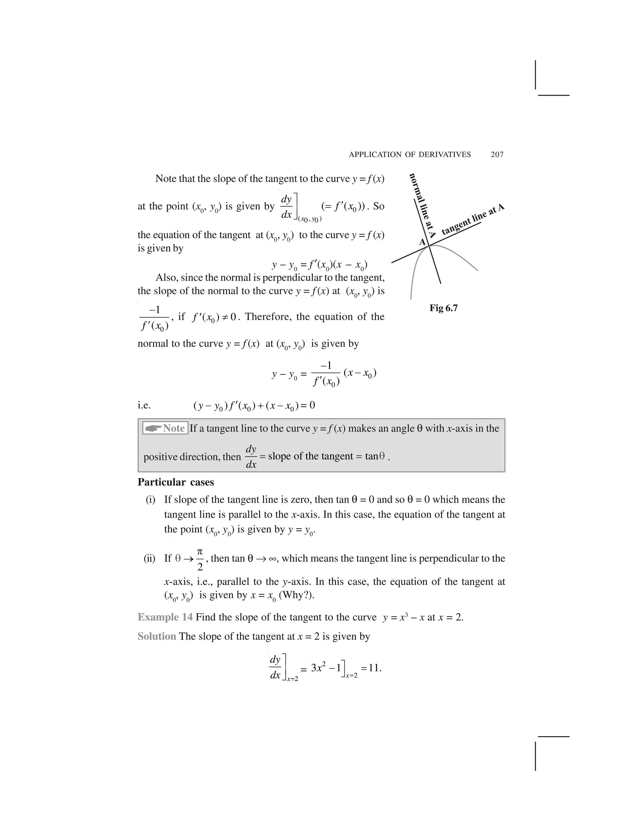
![MATHEMATICS218
Fig 6.9
Example 26 Find the maximum and the minimum values,
if any, of the function f given by
f (x) = x2
, x ☎R.
Solution From the graph of the given function (Fig 6.10),
we have f (x) = 0 if x = 0. Also
f (x) ✞0, for all x ☎R.
Therefore, the minimum value of f is 0 and the point
of minimum value of f is x = 0. Further, it may be observed
from the graph of the function that f has no maximum
value and hence no point of maximum value of f in R.
Note If we restrict the domain of f to [– 2, 1] only,
then f will have maximum value(– 2)2
= 4 at x = – 2.
Example 27 Find the maximum and minimum values
of f , if any, of the function given by f(x) = |x|, x ☎R.
Solution From the graph of the given function
(Fig 6.11) , note that
f (x) ✞0, for all x ☎R and f (x) = 0 if x = 0.
Therefore, the function f has a minimum value 0
and the point of minimum value of f is x = 0. Also, the
graph clearly shows that f has no maximum value in
R and hence no point of maximum value in R.
Note
(i) If we restrict the domain of f to [– 2, 1] only, then f will have maximum value
|– 2| = 2.
Fig 6.10
Fig 6.11](https://image.slidesharecdn.com/ncert-class-12-mathematics-part-1-161112165946/75/Ncert-class-12-mathematics-part-1-221-2048.jpg)
![APPLICATION OF DERIVATIVES 219
(ii) One may note that the function f in Example 27 is not differentiable at
x = 0.
Example 28 Find the maximum and the minimum values, if any, of the function
given by
f (x) = x, x ☎ (0, 1).
Solution The given function is an increasing (strictly) function in the given interval
(0, 1). From the graph (Fig 6.12) of the function f , it
seems that, it should have the minimum value at a
point closest to 0 on its right and the maximum value
at a point closest to 1 on its left. Are such points
available? Of course, not. It is not possible to locate
such points. Infact, if a point x0
is closest to 0, then
we find
0
0
2
x
x for all 0 (0,1)x ✁ . Also, if x1
is
closest to 1, then
1
1
1
2
x
x
✂
✄ for all 1 (0,1)x ✆ .
Therefore, the given function has neither the maximum value nor the minimum
value in the interval (0,1).
Remark The reader may observe that in Example 28, if we include the points 0 and 1
in the domain of f , i.e., if we extend the domain of f to [0,1], then the function f has
minimum value 0 at x = 0 and maximum value 1 at x = 1. Infact, we have the following
results (The proof of these results are beyond the scope of the present text)
Every monotonic function assumes its maximum/minimum value at the end
points of the domain of definition of the function.
A more general result is
Every continuous function on a closed interval has a maximum and a minimum
value.
✝Note By a monotonic function f in an interval I, we mean that f is either
increasing in I or decreasing in I.
Maximum and minimum values of a function defined on a closed interval will be
discussed later in this section.
Let us now examine the graph of a function as shown in Fig 6.13. Observe that at
points A, B, C and D on the graph, the function changes its nature from decreasing to
increasing or vice-versa. These points may be called turning points of the given
function. Further, observe that at turning points, the graph has either a little hill or a little
valley. Roughly speaking, the function has minimum value in some neighbourhood
(interval) of each of the points A and C which are at the bottom of their respective
Fig 6.12](https://image.slidesharecdn.com/ncert-class-12-mathematics-part-1-161112165946/75/Ncert-class-12-mathematics-part-1-222-2048.jpg)
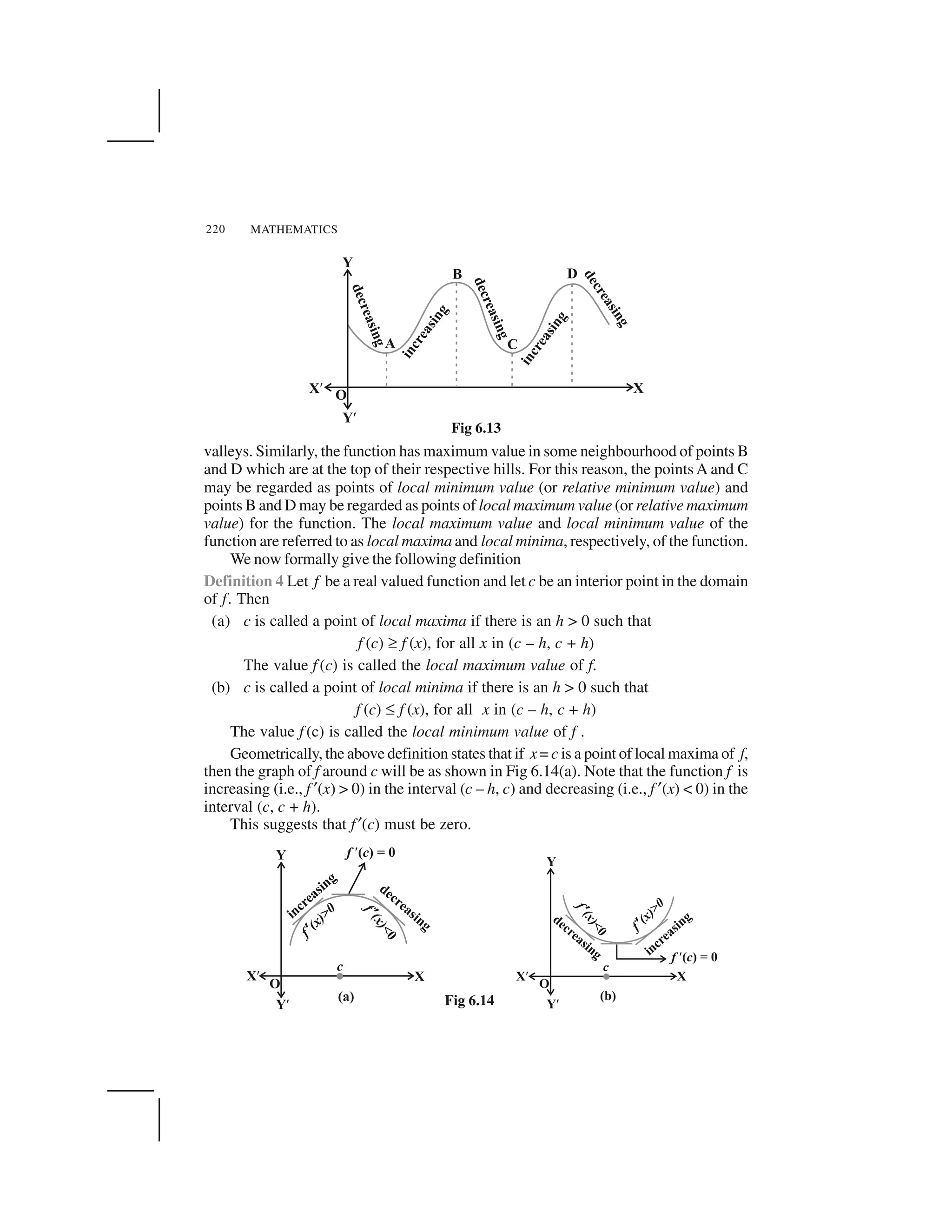
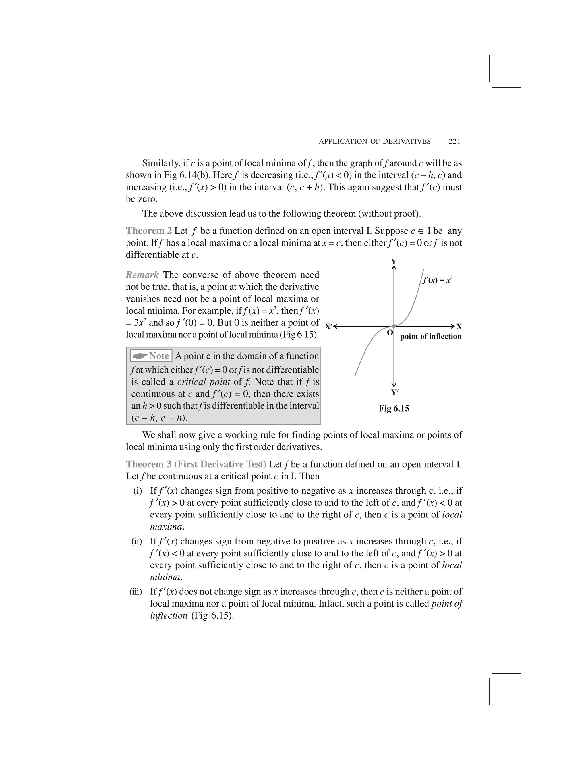
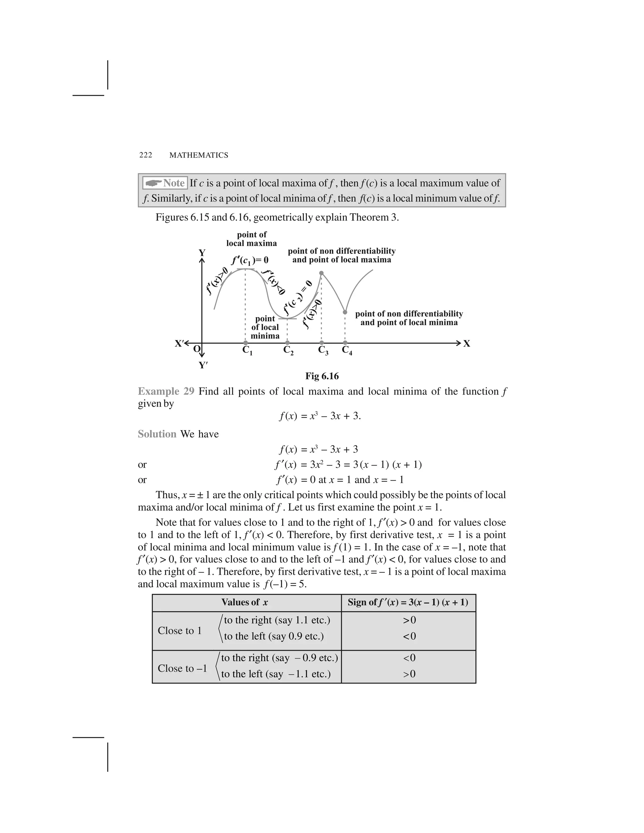
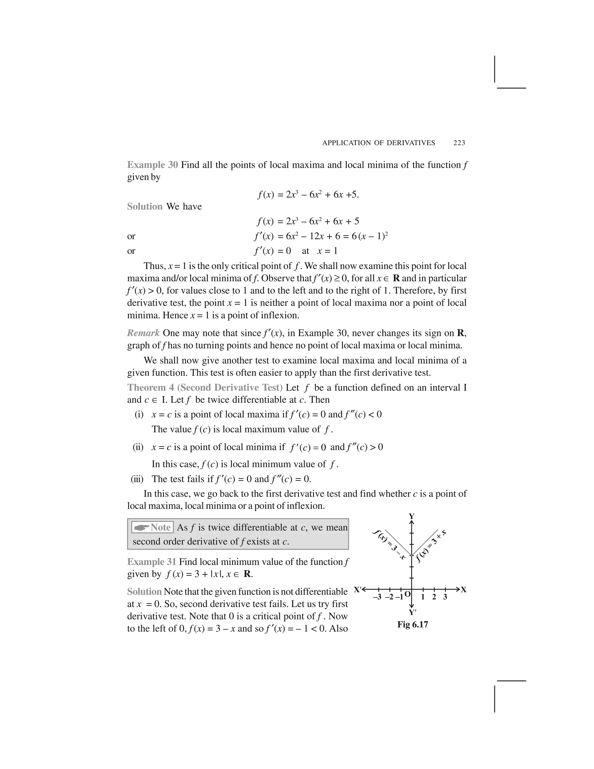
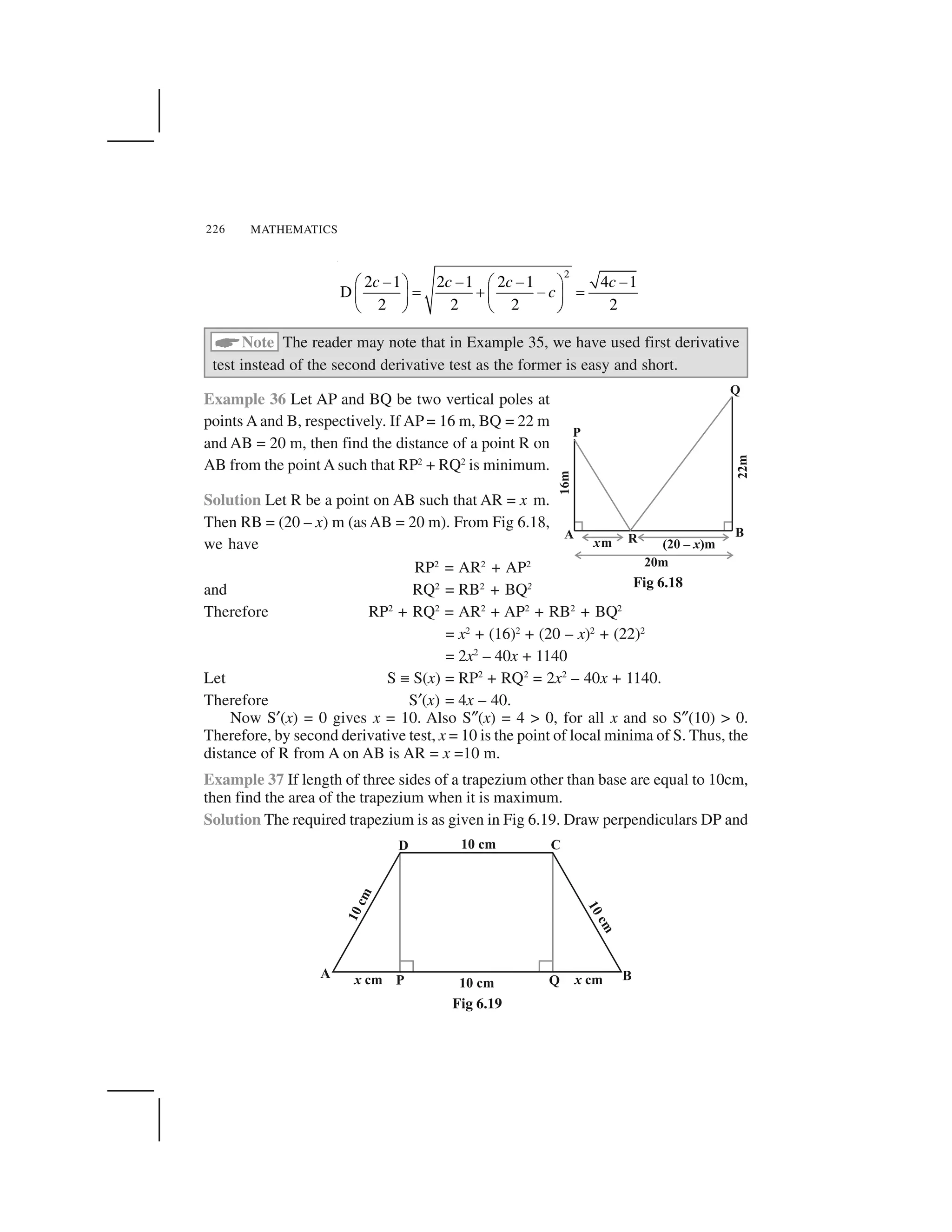
![MATHEMATICS228
QE
OA
=
EC
OC
(since ✌QEC ~ ✌AOC)
or
QE
h
=
r x
r
or QE =
( )h r x
r
Let S be the curved surface area of the given
cylinder. Then
S ✏ S(x) =
2 ( )xh r x
r
✁ ✂
=
22
( )
h
rx x
r
✁
✂
or
2
S ( ) ( 2 )
4
S ( )
h
x r x
r
h
x
r
✄☎ ✆ ✝ ✞✟✟
✠
✞ ✄✟ ✆✆ ✝
✟✡
Now S☛(x) = 0 gives
2
r
x ☞ . Since S✎(x) < 0 for all x, S 0
2
r✍ ✑✒✒ ✓✔ ✕
✖ ✗
. So
2
r
x ☞ is a
point of maxima of S. Hence, the radius of the cylinder of greatest curved surface area
which can be inscribed in a given cone is half of that of the cone.
6.6.1 Maximum and Minimum Values of a Function in a Closed Interval
Let us consider a function f given by
f (x) = x + 2, x ✘ (0, 1)
Observe that the function is continuous on (0, 1) and neither has a maximum value
nor has a minimum value. Further, we may note that the function even has neither a
local maximum value nor a local minimum value.
However, if we extend the domain of f to the closed interval [0, 1], then f still may
not have a local maximum (minimum) values but it certainly does have maximum value
3 = f (1) and minimum value 2 = f (0). The maximum value 3 of f at x = 1 is called
absolute maximum value (global maximum or greatest value) of f on the interval
[0, 1]. Similarly, the minimum value 2 of f at x = 0 is called the absolute minimum
value (global minimum or least value) of f on [0, 1].
Consider the graph given in Fig 6.21 of a continuous function defined on a closed
interval [a, d]. Observe that the function f has a local minima at x = b and local
Fig 6.20](https://image.slidesharecdn.com/ncert-class-12-mathematics-part-1-161112165946/75/Ncert-class-12-mathematics-part-1-231-2048.jpg)
![APPLICATION OF DERIVATIVES 229
minimum value is f(b). The function also has a local maxima at x = cand local maximum
value is f (c).
Also from the graph, it is evident that f has absolute maximum value f (a) and
absolute minimum value f (d). Further note that the absolute maximum (minimum)
value of f is different from local maximum (minimum) value of f.
We will now state two results (without proof) regarding absolute maximum and
absolute minimum values of a function on a closed interval I.
Theorem 5 Let f be a continuous function on an interval I = [a, b]. Then f has the
absolute maximum value and f attains it at least once in I. Also, f has the absolute
minimum value and attains it at least once in I.
Theorem 6 Let f be a differentiable function on a closed interval I and let c be any
interior point of I. Then
(i) f ✂(c) = 0 if f attains its absolute maximum value at c.
(ii) f ✂(c) = 0 if f attains its absolute minimum value at c.
In view of the above results, we have the following working rule for finding absolute
maximum and/or absolute minimum values of a function in a given closed interval
[a, b].
Working Rule
Step 1: Find all critical points of f in the interval, i.e., find points x where either
( ) 0f x ✁ or f is not differentiable.
Step 2: Take the end points of the interval.
Step 3: At all these points (listed in Step 1 and 2), calculate the values of f .
Step 4: Identify the maximum and minimum values of f out of the values calculated in
Step 3. This maximum value will be the absolute maximum (greatest) value of
f and the minimum value will be the absolute minimum (least) value of f .
Fig 6.21](https://image.slidesharecdn.com/ncert-class-12-mathematics-part-1-161112165946/75/Ncert-class-12-mathematics-part-1-232-2048.jpg)
![MATHEMATICS230
Example 39 Find the absolute maximum and minimum values of a function f given by
f (x) = 2x3
– 15x2
+ 36x +1 on the interval [1, 5].
Solution We have
f (x) = 2x3
– 15x2
+ 36x + 1
or f ✂(x) = 6x2
– 30x + 36 = 6 (x – 3) (x – 2)
Note that f ✂(x) = 0 gives x = 2 and x = 3.
We shall now evaluate the value of f at these points and at the end points of the
interval [1, 5], i.e., at x = 1, x = 2, x = 3 and at x = 5. So
f (1) = 2(13
) – 15(12
) + 36 (1) + 1 = 24
f (2) = 2(23
) – 15(22
) + 36 (2) + 1 = 29
f (3) = 2(33
) – 15(32
) + 36 (3) + 1 = 28
f (5) = 2(53
) – 15(52
) + 36 (5) + 1 = 56
Thus, we conclude that absolute maximum value of f on [1, 5] is 56, occurring at
x =5, and absolute minimum value of f on [1, 5] is 24 which occurs at x = 1.
Example 40 Find absolute maximum and minimum values of a function f given by
4 1
3 3( ) 12 6 , [ 1, 1]f x x x x ✁ ✄ ✁
Solution We have
f (x) =
4 1
3 312 6x x☎
or f ✂(x) =
1
3
2 2
3 3
2 2(8 1)
16
x
x
x x
✆
✆ ✝
Thus, f ✂(x) = 0 gives
1
8
x ✞ . Further note that f ✂(x) is not defined at x = 0. So the
critical points are x = 0 and
1
8
x ✞ . Now evaluating the value of f at critical points
x = 0,
1
8
and at end points of the interval x = –1 and x = 1, we have
f (–1) =
4 1
3 312( 1) 6( 1) 18✁ ✁ ✁
f (0) = 12 (0) – 6(0) = 0](https://image.slidesharecdn.com/ncert-class-12-mathematics-part-1-161112165946/75/Ncert-class-12-mathematics-part-1-233-2048.jpg)
![MATHEMATICS232
2. Find the maximum and minimum values, if any, of the following functions
given by
(i) f (x) = |x + 2| – 1 (ii) g(x) = – |x + 1| + 3
(iii) h(x) = sin(2x) + 5 (iv) f (x) = |sin 4x + 3|
(v) h(x) = x + 1, x ☎ (– 1, 1)
3. Find the local maxima and local minima, if any, of the following functions. Find
also the local maximum and the local minimum values, as the case may be:
(i) f (x) = x2
(ii) g(x) = x3
– 3x
(iii) h(x) = sin x + cos x,0
2
x
✁ ✁
(iv) f (x) = sin x – cos x, 0 2x✂ ✂ ✄
(v) f (x) = x3
– 6x2
+ 9x + 15 (vi)
2
( ) , 0
2
x
g x x
x
✆ ✝ ✞
(vii) 2
1
( )
2
g x
x
✟
✠
(viii) ( ) 1 , 0f x x x x✟ ✡ ☛
4. Prove that the following functions do not have maxima or minima:
(i) f (x) = ex
(ii) g(x) = log x
(iii) h (x) = x3
+ x2
+ x +1
5. Findtheabsolutemaximumvalueandtheabsoluteminimumvalueofthefollowing
functions in the given intervals:
(i) f (x) = x3
, x ☎ [– 2, 2] (ii) f (x) = sin x + cos x , x ☎ [0, ☞]
(iii) f (x) = 21 9
4 , 2,
2 2
x x x
✌ ✍
✎ ✏ ✎✑ ✒✓ ✔
(iv) 2
( ) ( 1) 3, [ 3,1]f x x x✟ ✡ ✠ ✕ ✡
6. Find the maximum profit that a company can make, if the profit function is
given by
p(x) = 41 – 24x – 18x2
7. Find both the maximum value and the minimum value of
3x4
– 8x3
+ 12x2
– 48x + 25 on the interval [0, 3].
8. At what points in the interval [0, 2☞], does the function sin 2x attain its maximum
value?
9. What is the maximum value of the function sin x + cos x?
10. Find the maximum value of 2x3
– 24x + 107 in the interval [1, 3]. Find the
maximum value of the same function in [–3, –1].](https://image.slidesharecdn.com/ncert-class-12-mathematics-part-1-161112165946/75/Ncert-class-12-mathematics-part-1-235-2048.jpg)
![APPLICATION OF DERIVATIVES 233
11. It is given that at x = 1, the function x4
– 62x2
+ ax + 9 attains its maximum value,
on the interval [0, 2]. Find the value of a.
12. Find the maximum and minimum values of x + sin 2x on [0, 2✄].
13. Find two numbers whose sum is 24 and whose product is as large as possible.
14. Find two positive numbers x and y such that x + y = 60 and xy3
is maximum.
15. Find two positive numbers x and y such that their sum is 35 and the product x2
y5
is a maximum.
16. Find two positive numbers whose sum is 16 and the sum of whose cubes is
minimum.
17. A square piece of tin of side 18 cm is to be made into a box without top, by
cutting a square from each corner and folding up the flaps to form the box. What
should be the side of the square to be cut off so that the volume of the box is the
maximum possible.
18. A rectangular sheet of tin 45 cm by 24 cm is to be made into a box without top,
by cutting off square from each corner and folding up the flaps. What should be
the side of the square to be cut off so that the volume of the box is maximum ?
19. Show that of all the rectangles inscribed in a given fixed circle, the square has
the maximum area.
20. Show that the right circular cylinder of given surface and maximum volume is
such that its height is equal to the diameter of the base.
21. Of all the closed cylindrical cans (right circular), of a given volume of 100 cubic
centimetres, find the dimensions of the can which has the minimum surface
area?
22. A wire of length 28 m is to be cut into two pieces. One of the pieces is to be
made into a square and the other into a circle. What should be the length of the
two pieces so that the combined area of the square and the circle is minimum?
23. Prove that the volume of the largest cone that can be inscribed in a sphere of
radius R is
8
27
of the volume of the sphere.
24. Show that the right circular cone of least curved surface and given volume has
an altitude equal to 2 time the radius of the base.
25. Show that the semi-vertical angle of the cone of the maximum volume and of
given slant height is 1
tan 2
.
26. Show that semi-vertical angle of right circular cone of given surface area and
maximum volume is 1 1
sin
3
✁ ✂ ☎
✆ ✝
✞ ✟
.](https://image.slidesharecdn.com/ncert-class-12-mathematics-part-1-161112165946/75/Ncert-class-12-mathematics-part-1-236-2048.jpg)
![MATHEMATICS234
Choose the correct answer in the Exercises 27 and 29.
27. The point on the curve x2
= 2y which is nearest to the point (0, 5) is
(A) (2 2,4) (B) (2 2,0) (C) (0, 0) (D) (2, 2)
28. For all real values of x, the minimum value of
2
2
1
1
x x
x x
✁
✁ ✁
is
(A) 0 (B) 1 (C) 3 (D)
1
3
29. The maximum value of
1
3[ ( 1) 1]x x ✂ ✄ , 0 1x☎ ☎ is
(A)
1
31
3
✆ ✝
✞ ✟✠ ✡
(B)
1
2
(C) 1 (D) 0
Miscellaneous Examples
Example 42 Acar starts from a point P at time t = 0 seconds and stops at point Q. The
distance x, in metres, covered by it, in t seconds is given by
2
2
3
t
x t
☛ ☞
✌ ✍✎ ✏✑ ✒
Find the time taken by it to reach Q and also find distance between P and Q.
Solution Let v be the velocity of the car at t seconds.
Now x = 2
2
3
t
t
☛ ☞
✍✎ ✏
✑ ✒
Therefore v =
dx
dt
= 4t – t2
= t(4 – t)
Thus, v = 0 gives t = 0 and/or t = 4.
Now v = 0 at P as well as at Q and at P, t = 0. So, at Q, t = 4. Thus, the car will
reach the point Q after 4 seconds. Also the distance travelled in 4 seconds is given by
x]t = 4
=
2 4 2 32
4 2 16 m
3 3 3
✓ ✔ ✓ ✔
✕ ✕✖ ✗ ✖ ✗
✘ ✙ ✘ ✙](https://image.slidesharecdn.com/ncert-class-12-mathematics-part-1-161112165946/75/Ncert-class-12-mathematics-part-1-237-2048.jpg)
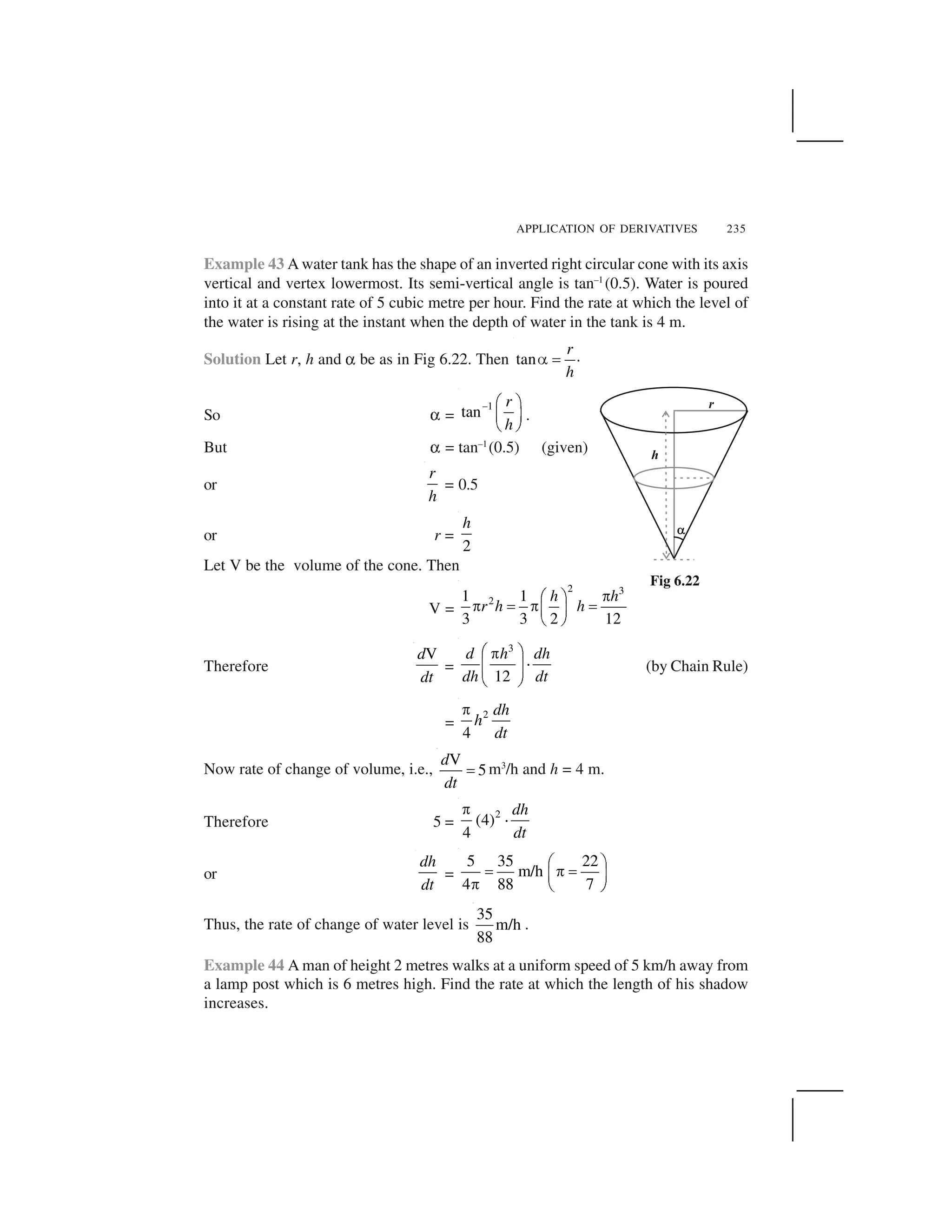
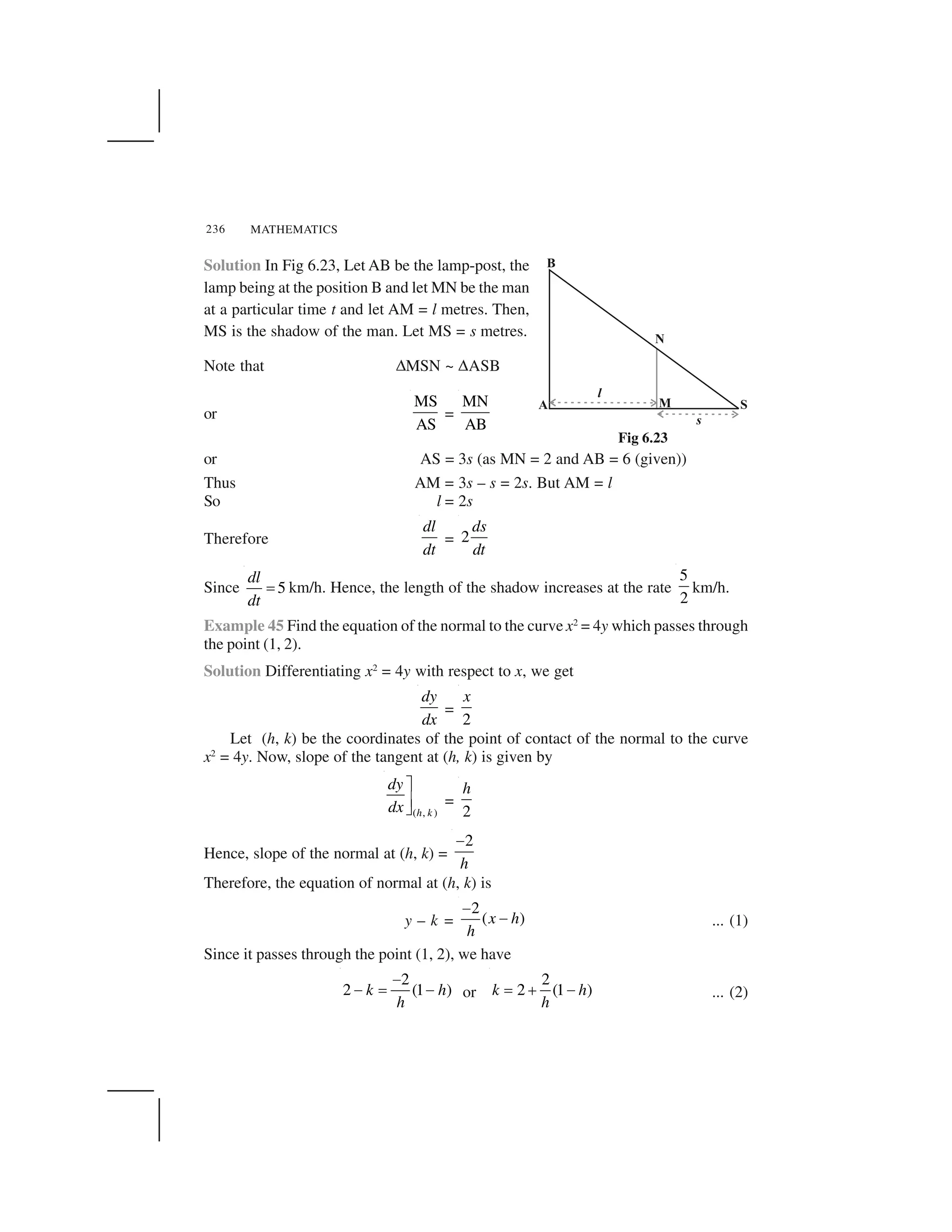
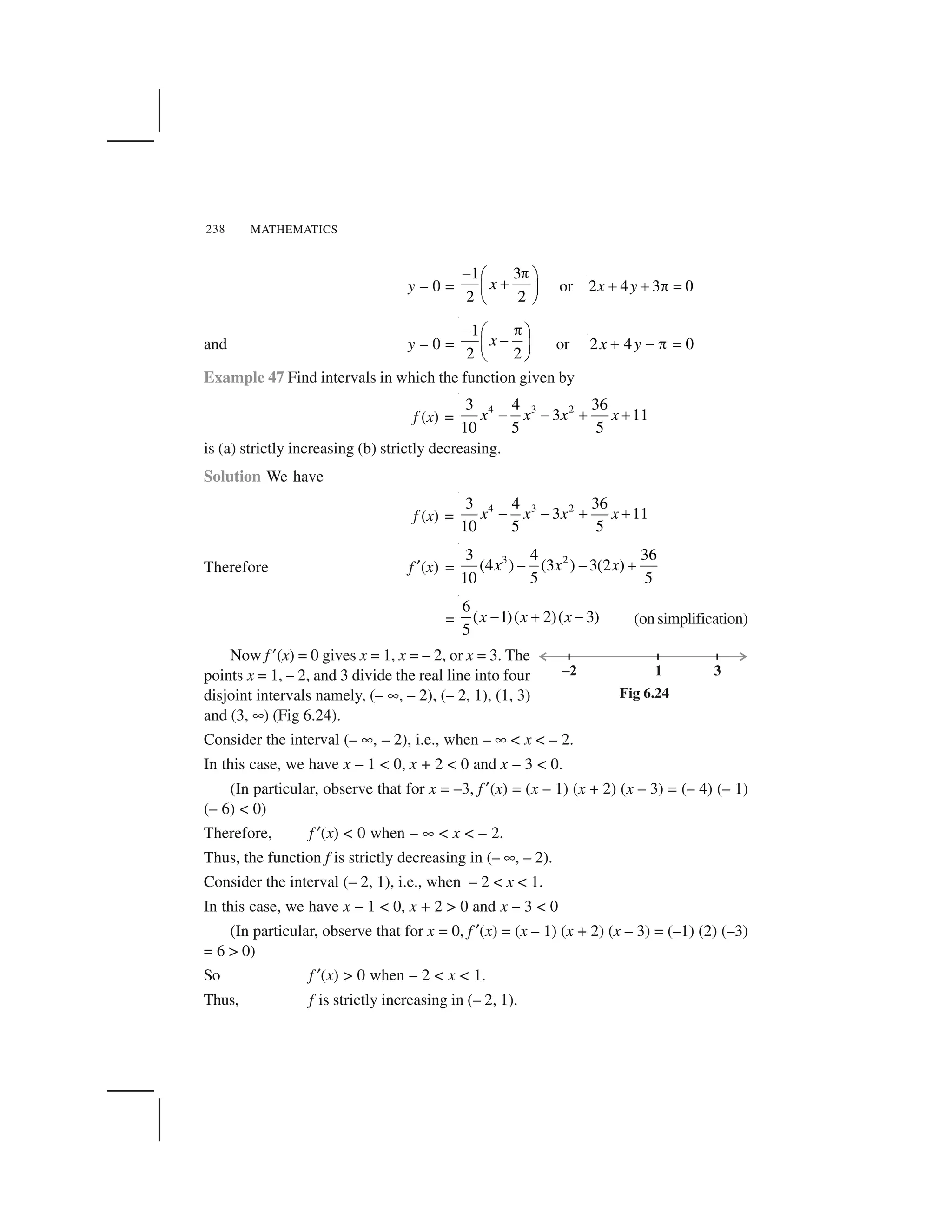
![APPLICATION OF DERIVATIVES 243
11. A window is in the form of a rectangle surmounted by a semicircular opening.
The total perimeter of the window is 10 m. Find the dimensions of the window to
admit maximum light through the whole opening.
12. A point on the hypotenuse of a triangle is at distance a and b from the sides of
the triangle.
Show that the maximum length of the hypotenuse is
2 2 3
3 3 2( )a b .
13. Find the points at which the function f given by f (x) = (x – 2)4
(x + 1)3
has
(i) local maxima (ii) localminima
(iii) point of inflexion
14. Find the absolute maximum and minimum values of the function f given by
f (x) = cos2
x + sin x, x ☎ [0, ✄]
15. Show that the altitude of the right circular cone of maximum volume that can be
inscribed in a sphere of radius r is
4
3
r
.
16. Let f be a function defined on [a, b] such that f ✂(x) > 0, for all x ☎ (a, b). Then
prove that f is an increasing function on (a, b).
17. Show that the height of the cylinder of maximum volume that can be inscribed in
a sphere of radius R is
2R
3
. Also find the maximum volume.
18. Show that height of the cylinder of greatest volume which can be inscribed in a
right circular cone of height h and semi vertical angle ✑ is one-third that of the
cone and the greatest volume of cylinder is
3 24
tan
27
h✁ ✆ .
Choose the correct answer in the Exercises from 19 to 24.
19. A cylindrical tank of radius 10 m is being filled with wheat at the rate of 314
cubic metre per hour. Then the depth of the wheat is increasing at the rate of
(A) 1 m3
/h (B) 0.1 m3
/h
(C) 1.1 m3
/h (D) 0.5 m3
/h
20. The slope of the tangent to the curve x = t2
+ 3t – 8, y = 2t2
– 2t – 5 at the point
(2,– 1) is
(A)
22
7
(B)
6
7
(C)
7
6
(D)
6
7
✝](https://image.slidesharecdn.com/ncert-class-12-mathematics-part-1-161112165946/75/Ncert-class-12-mathematics-part-1-246-2048.jpg)
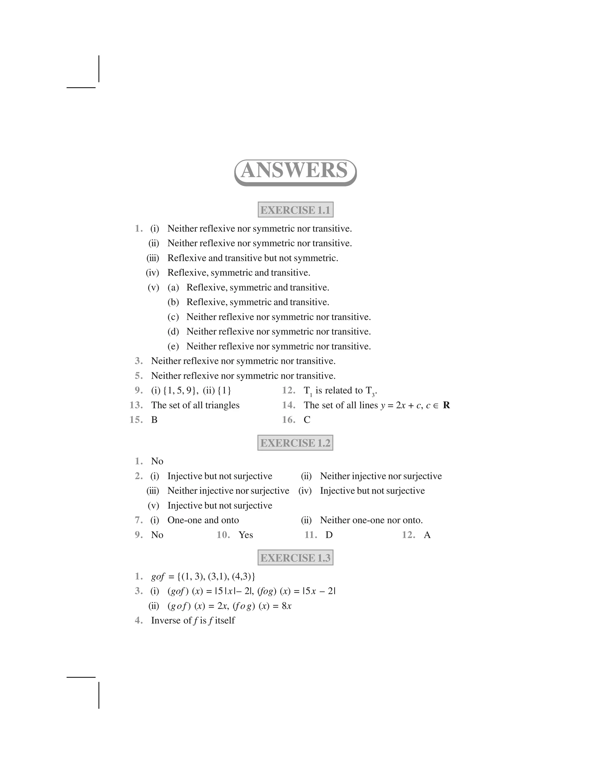
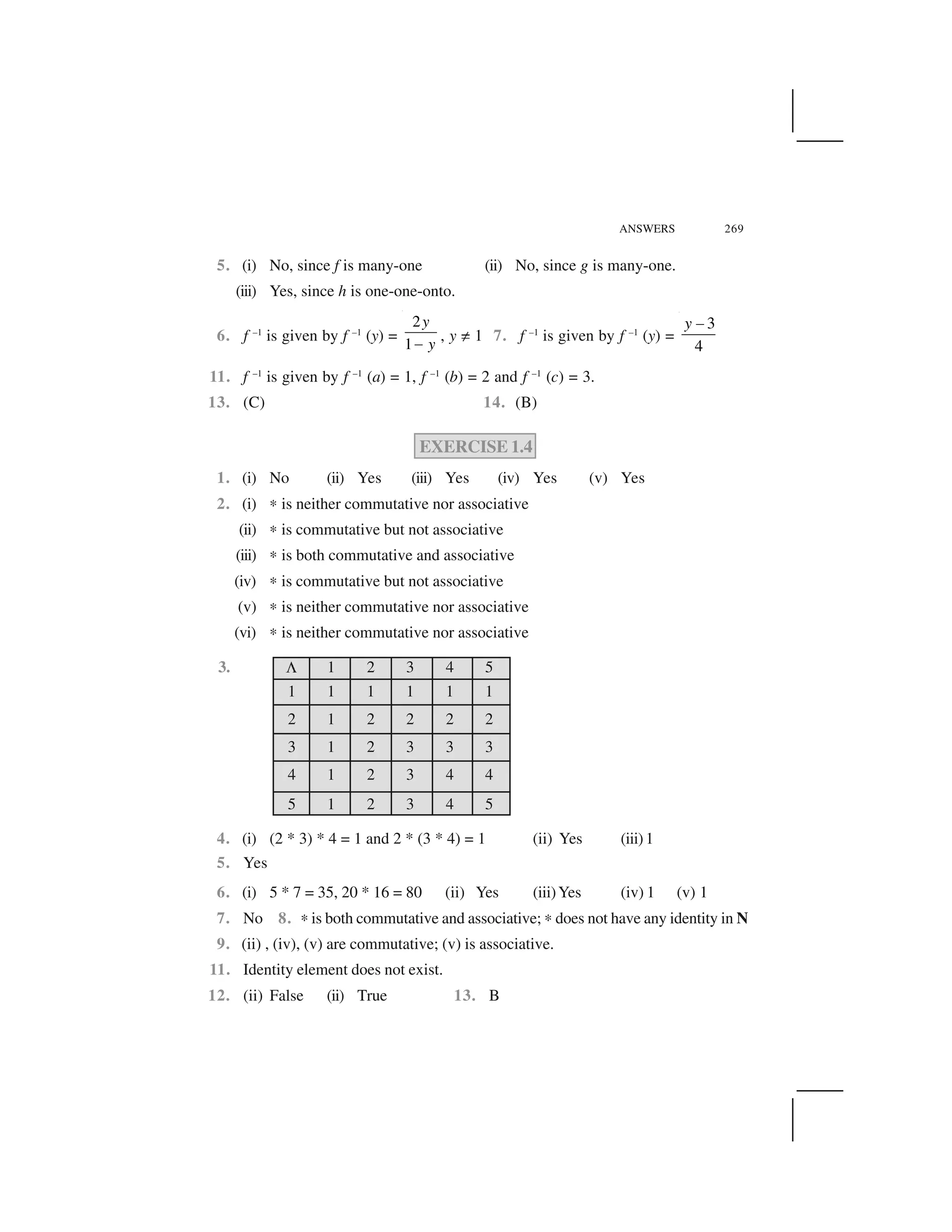
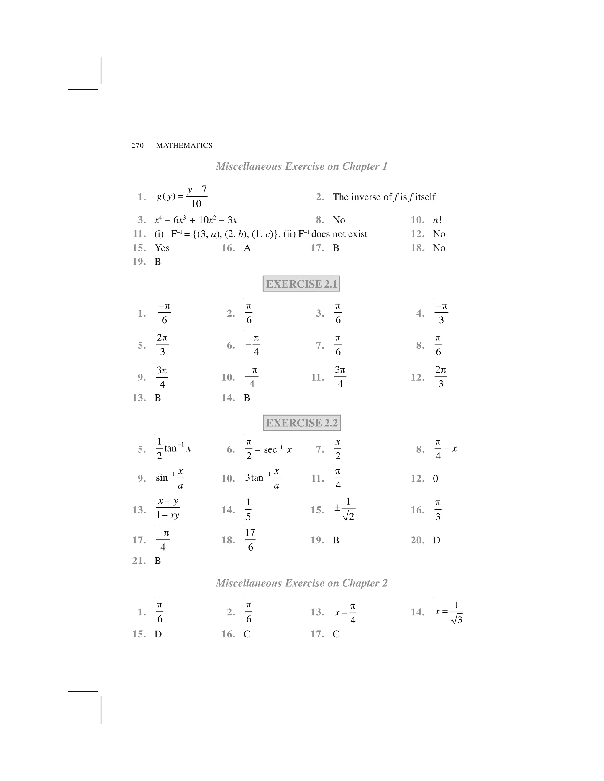
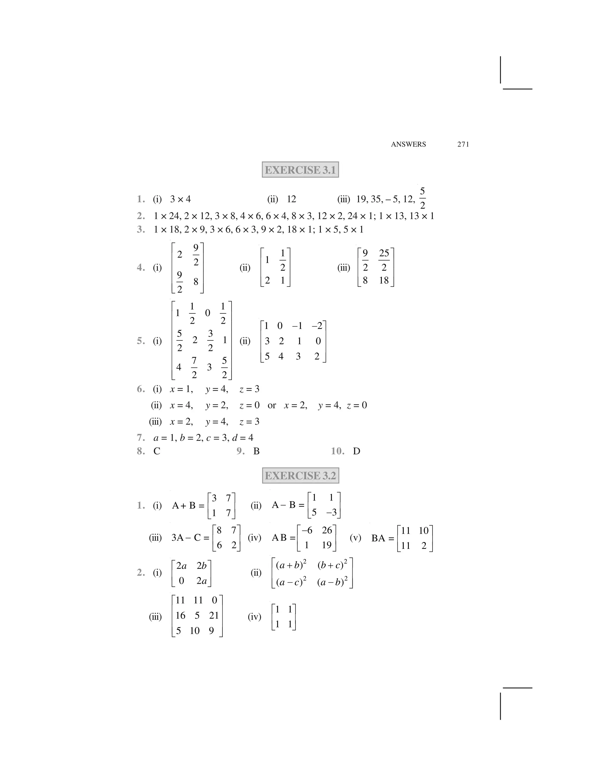
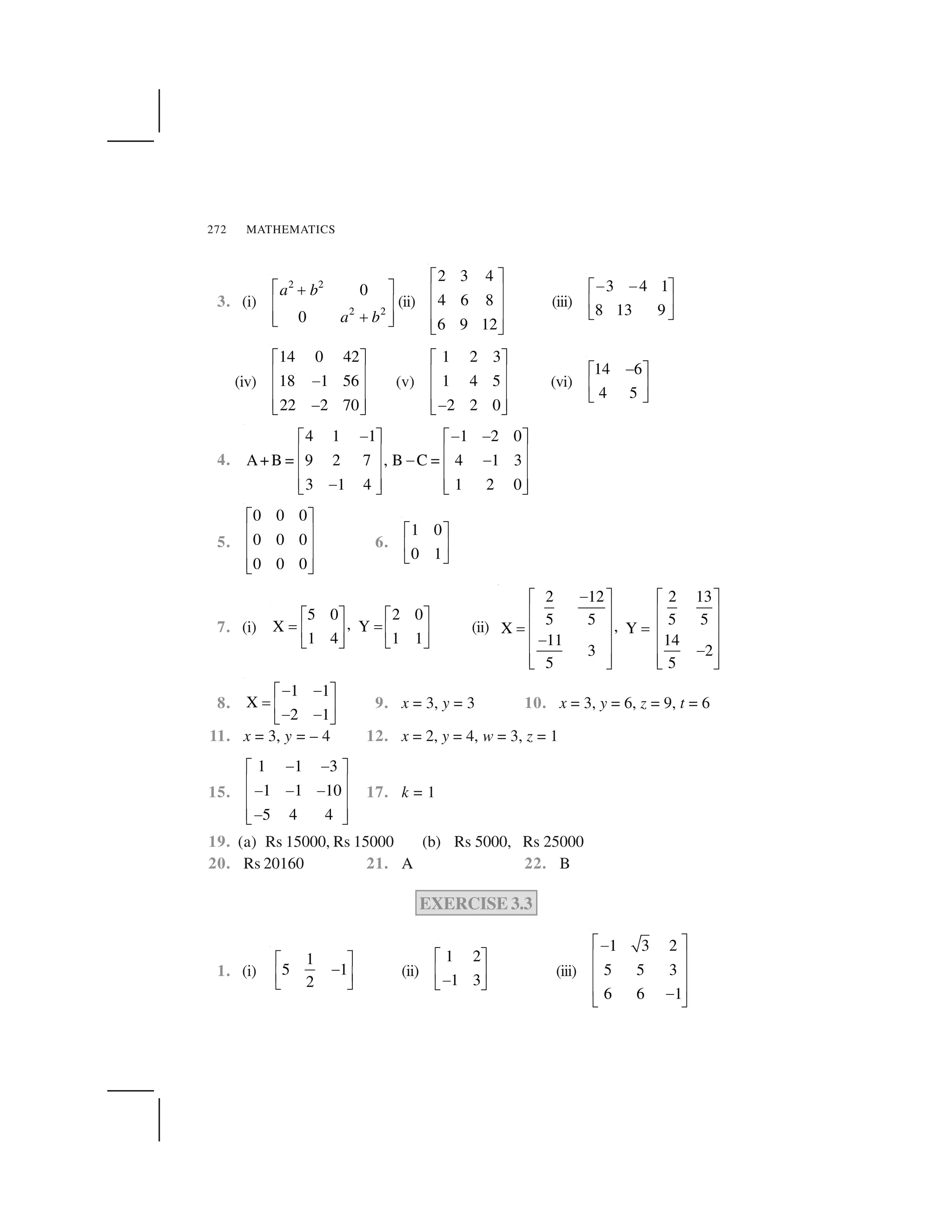
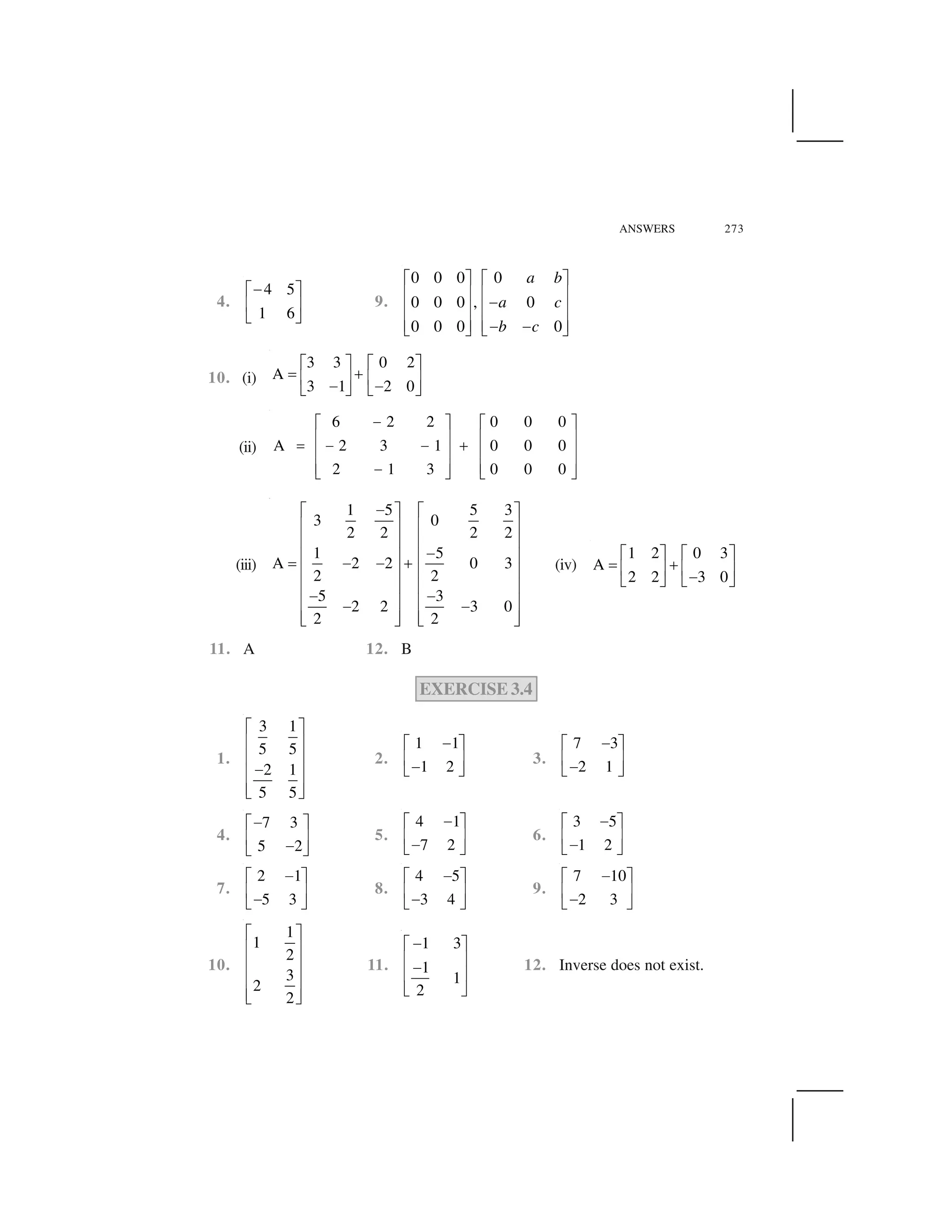
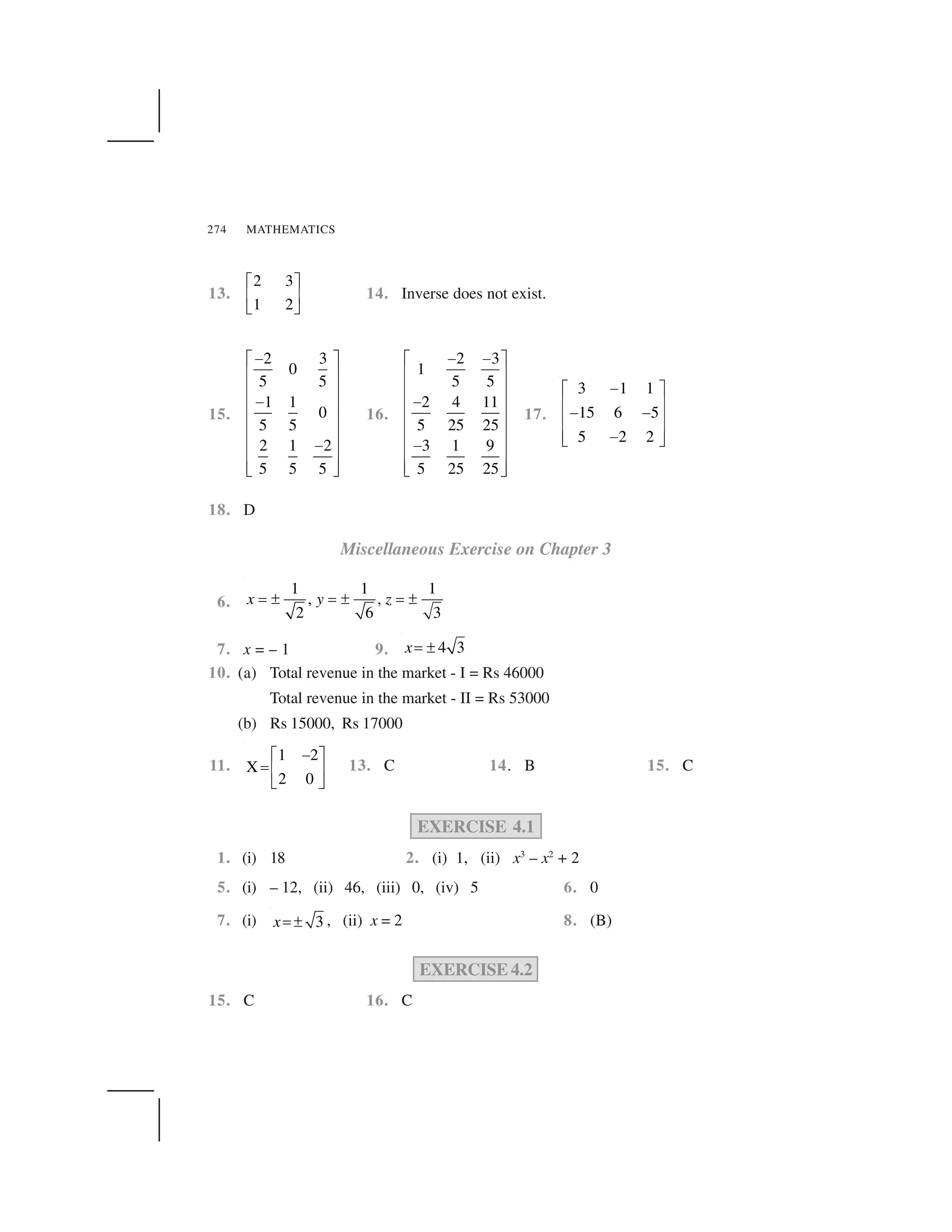
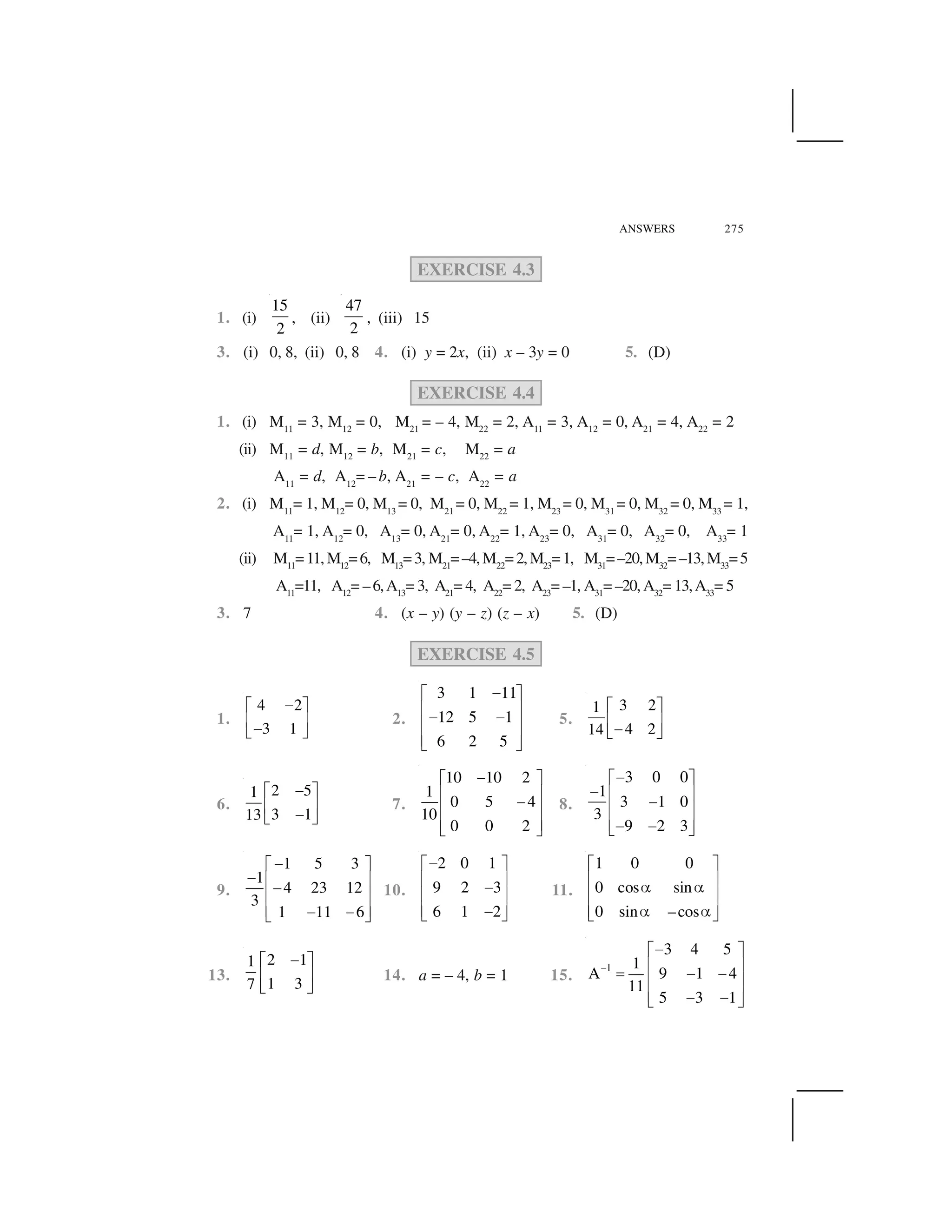
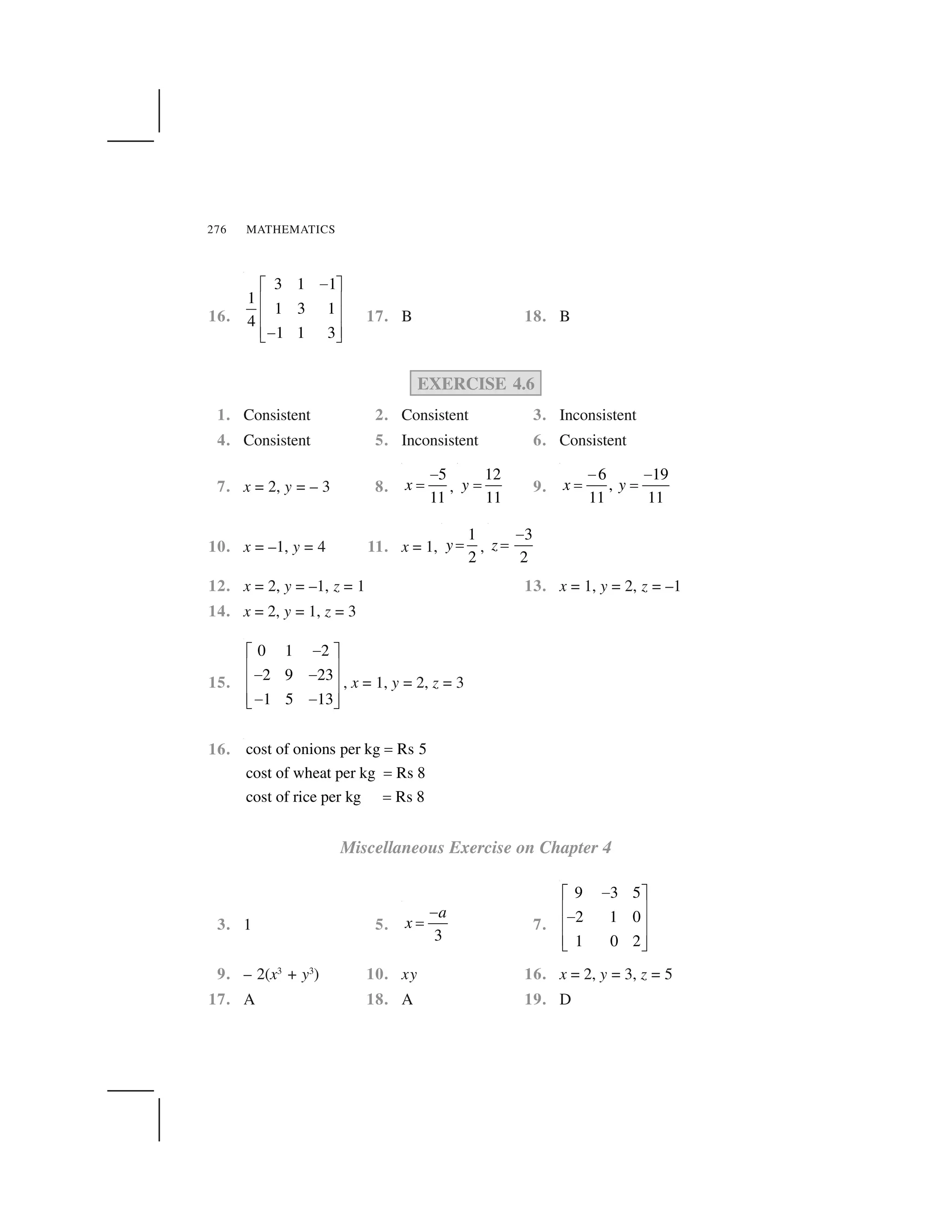

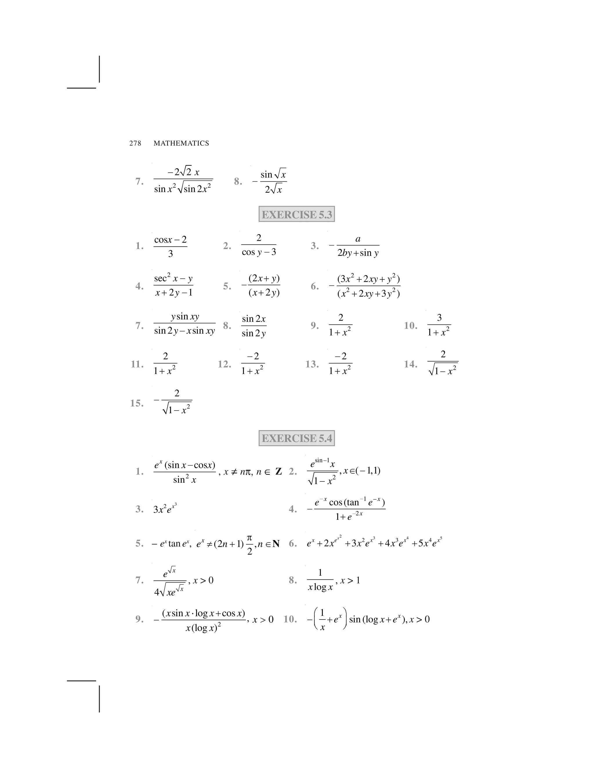
![ANSWERS 279
EXERCISE 5.5
1. – cos x cos 2x cos 3x [tan x + 2 tan 2x + 3 tan 3x]
2.
1 ( 1)( 2) 1 1 1 1 1
2 ( 3)( 4)( 5) 1 2 3 4 5
x x
x x x x x x x x
✁✂ ✂
✄ ✂ ✂ ✂☎ ✆
✂ ✂ ✂ ✂ ✂ ✂ ✂ ✂✝ ✞
3.
cos cos
(log ) sin log(log )
log
x x
x x x
x x
✟ ✠
✡☛ ☞
✌ ✍
4. xx
(1 + log x) – 2sin x
cos x log 2
5. (x + 3) (x + 4)2
(x + 5)3
(9x2
+ 70x + 133)
6.
12 1
2 2
1 1 1 1 log
log( )
1
x
x
x x x
x x x
x xx x
✎✏ ✑✒ ✓ ✒✔ ✕ ✔ ✕
✓ ✓ ✓ ✓✖ ✗✘ ✙ ✘ ✙
✓✚ ✛ ✚ ✛✜ ✢
7. (log x)x-1
[1 + log x . log (log x)] + 2xlogx–1
. logx
8. (sin x)x
(x cot x + log sin x) + 2
1 1
2 x x✣
9. x sinx sin
cos log
x
x x
x
✤ ✥
✦
✧ ★
✩ ✪
+ (sin x)cos x
[cos x cot x – sin x log sin x]
10. x x cosx
[cos x . (1 + log x) – x sin x log x] – 2 2
4
( 1)
x
x ✫
11. (x cos x)x
[1 – x tan x + log (x cos x)] + (x sin x)
1
2
cot 1 log( sin )x
x x x x
x
✄ ✂ ✁
☎ ✆
✝ ✞
12.
1
1
log
log
y x
y x
yx y y
x x xy
✬
✬
✭
✡
✭
13.
log
log
y y x y
x x y x
✮ ✯✰
✱ ✲
✰✳ ✴
14.
tan logcos
tan logcos
y x y
x y x
✵
✵
15.
( 1)
( 1)
y x
x y
✶
✵
16. (1 + x) (1 + x2
) (1 +x4
) (1 + x8
)
3 7
2 4 8
1 2 4 8
1 1 1 1
x x x
x x x x
✟ ✠
✭ ✭ ✭☛ ☞
✭ ✭ ✭ ✭✌ ✍
; f ✷(1) = 120
17. 5x4
– 20x3
+ 45x2
– 52x + 11
EXERCISE 5.6
1. 2t2
2.
b
a
3. – 4 sin t 4. 2
1
t
✒](https://image.slidesharecdn.com/ncert-class-12-mathematics-part-1-161112165946/75/Ncert-class-12-mathematics-part-1-261-2048.jpg)
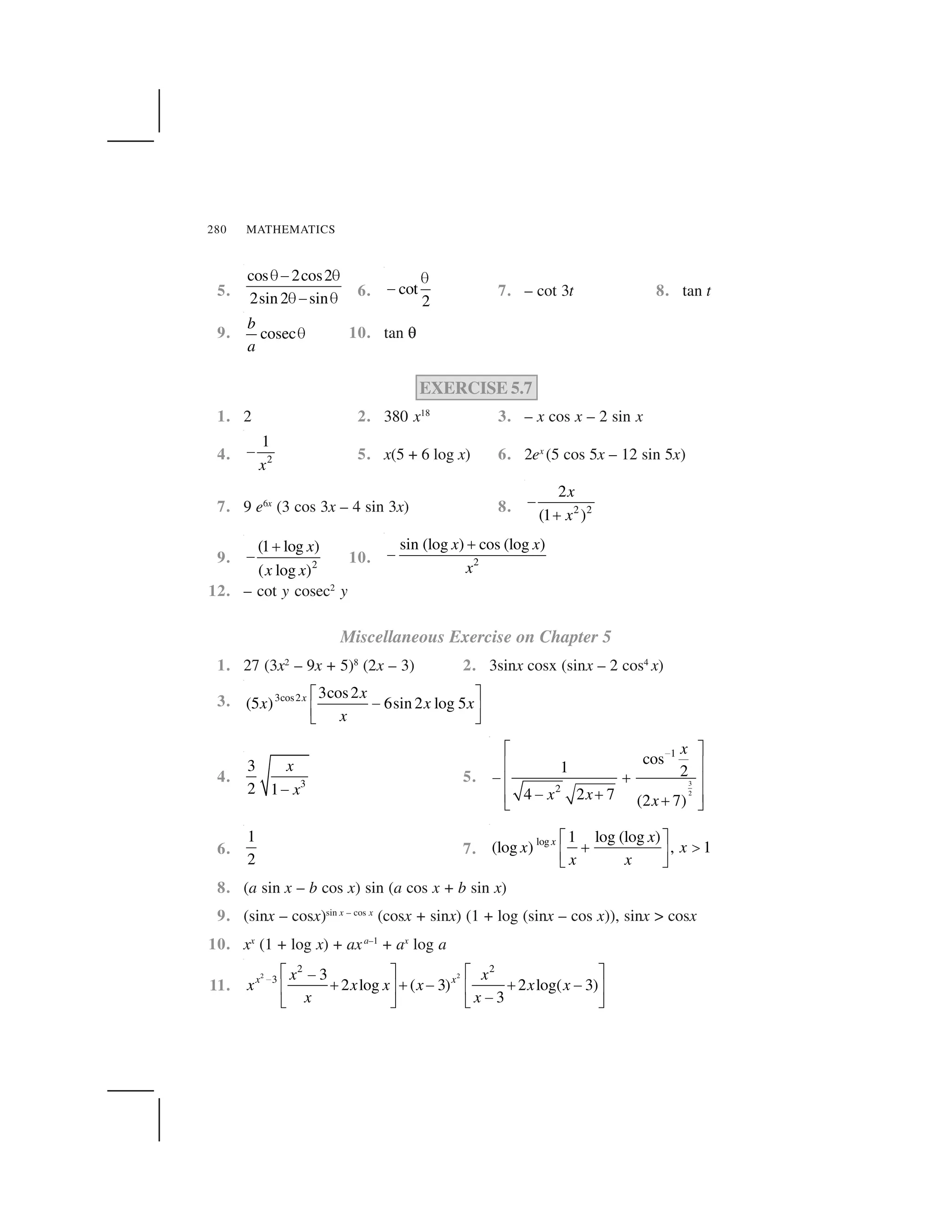
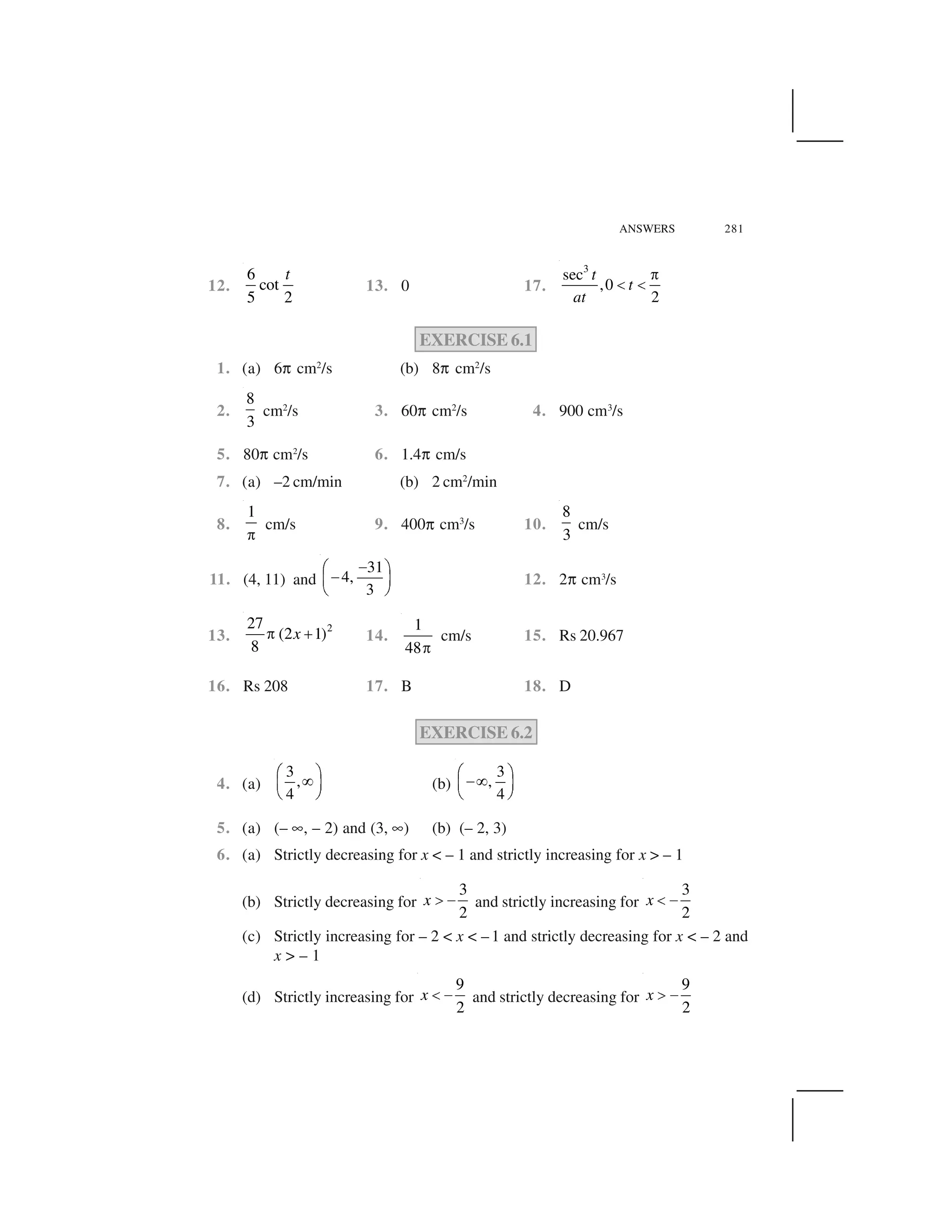
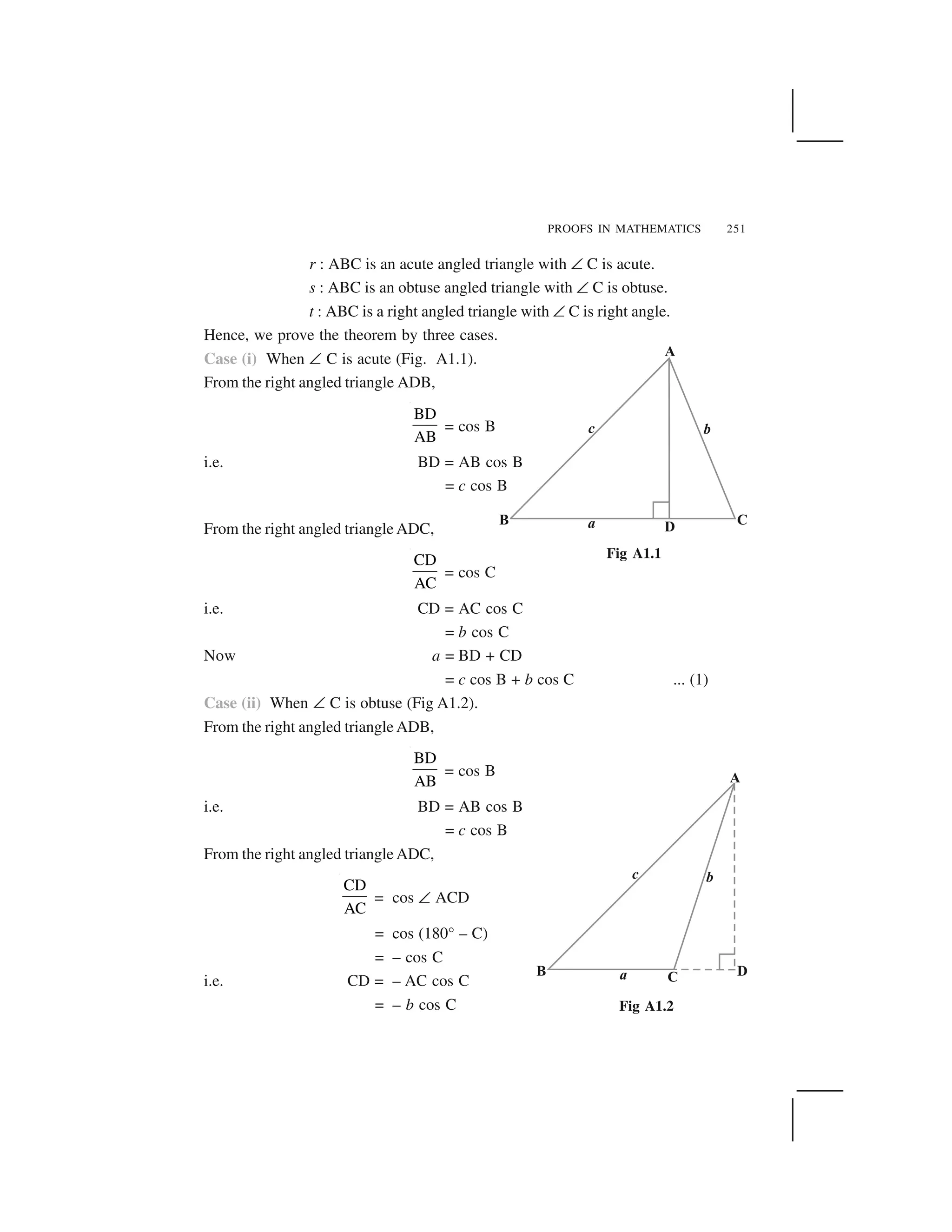
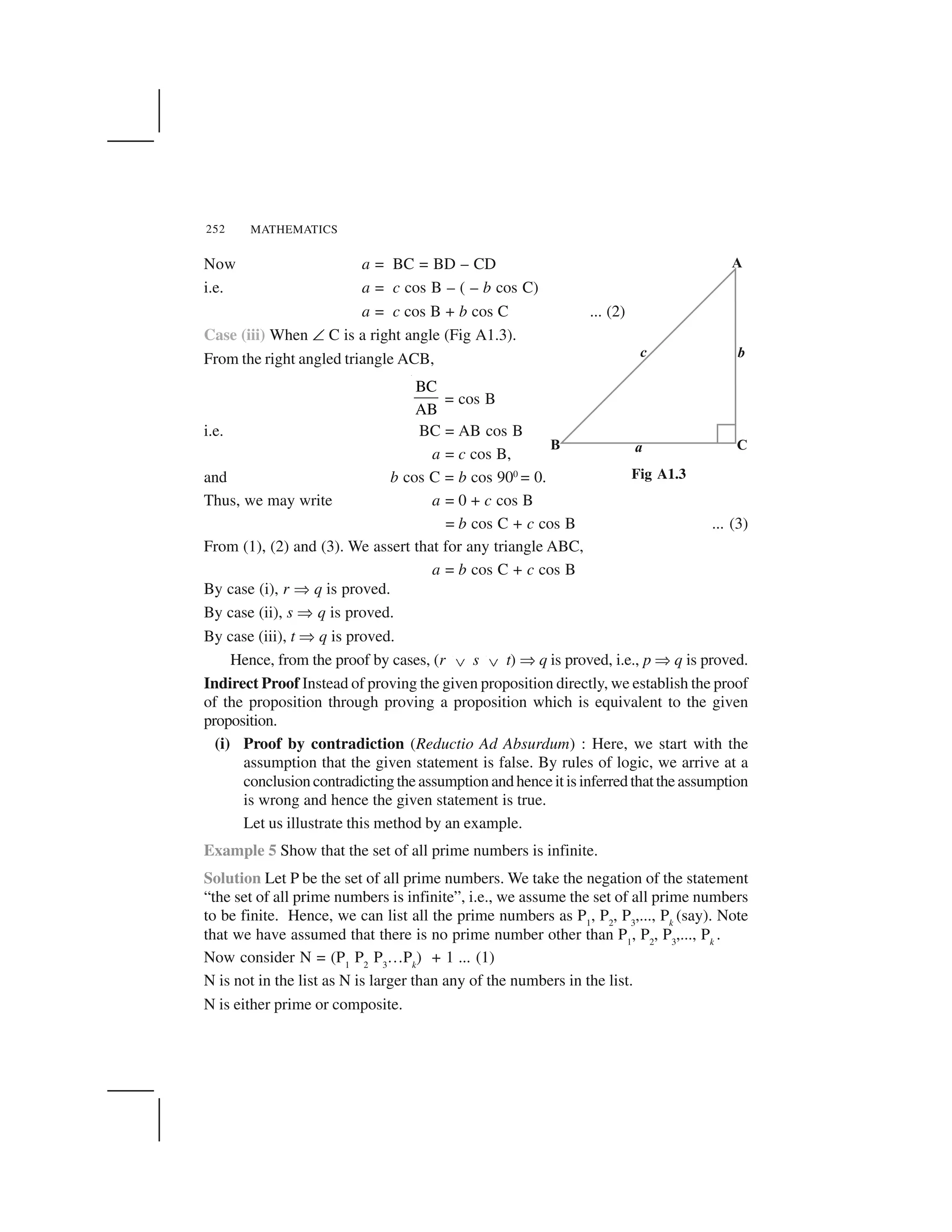
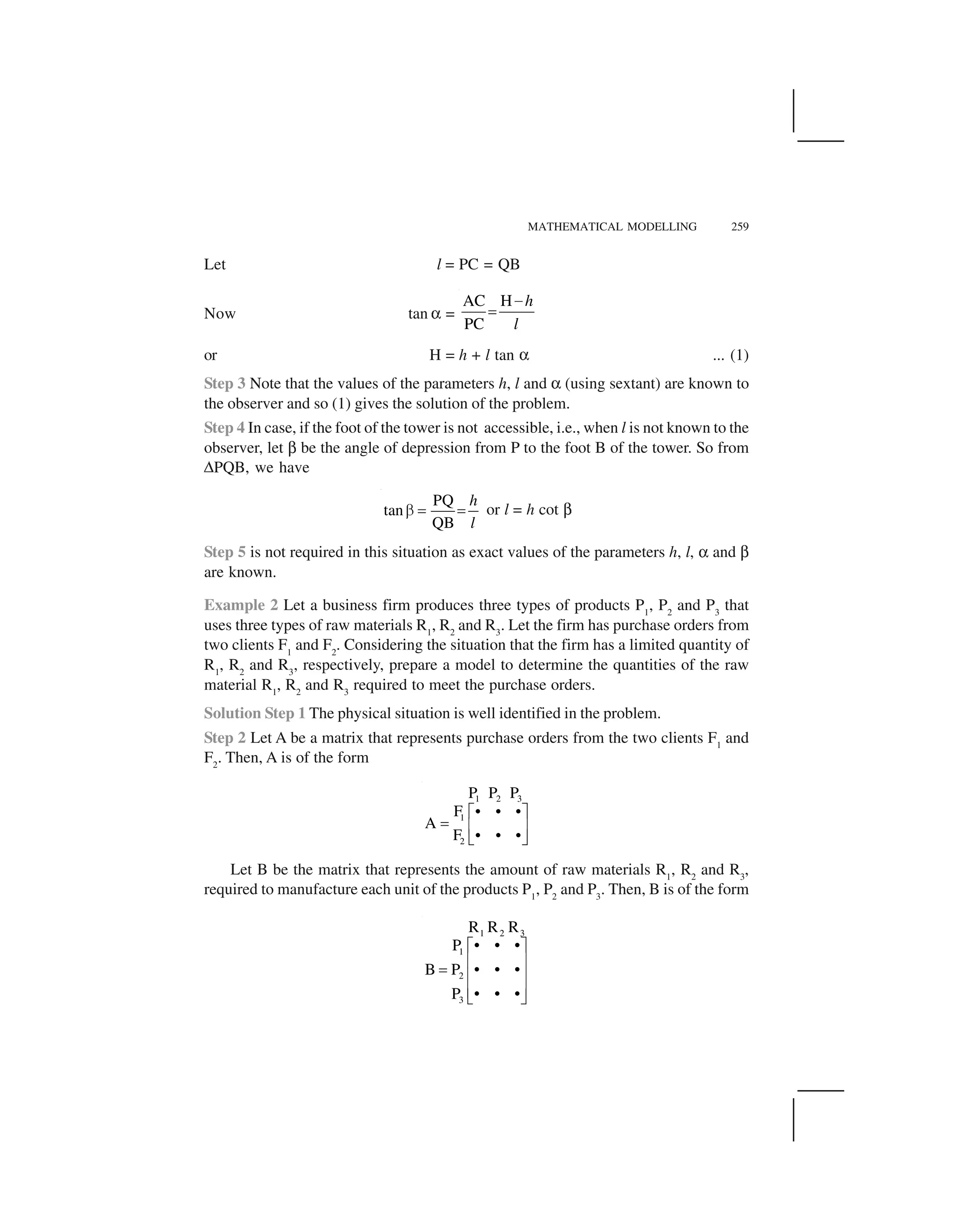
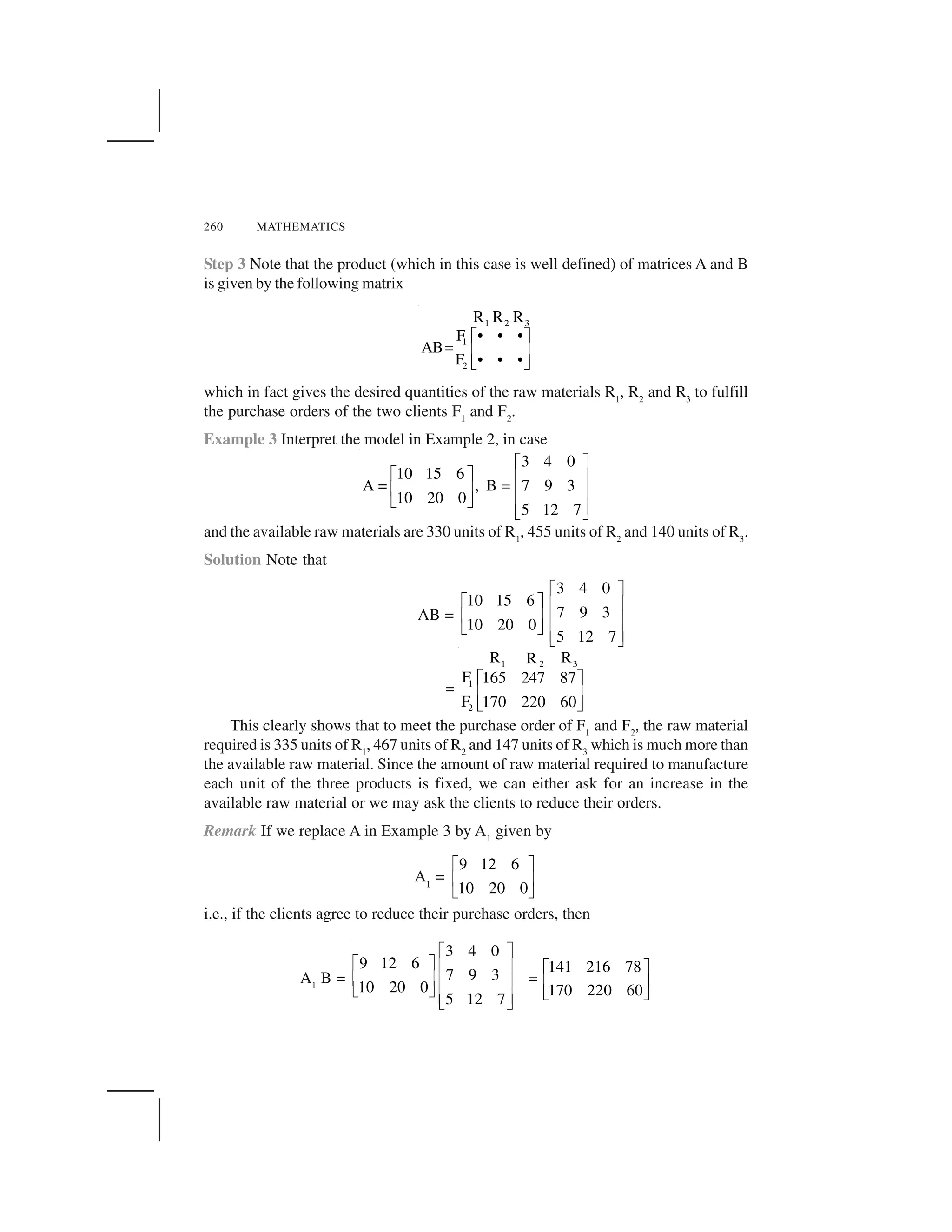
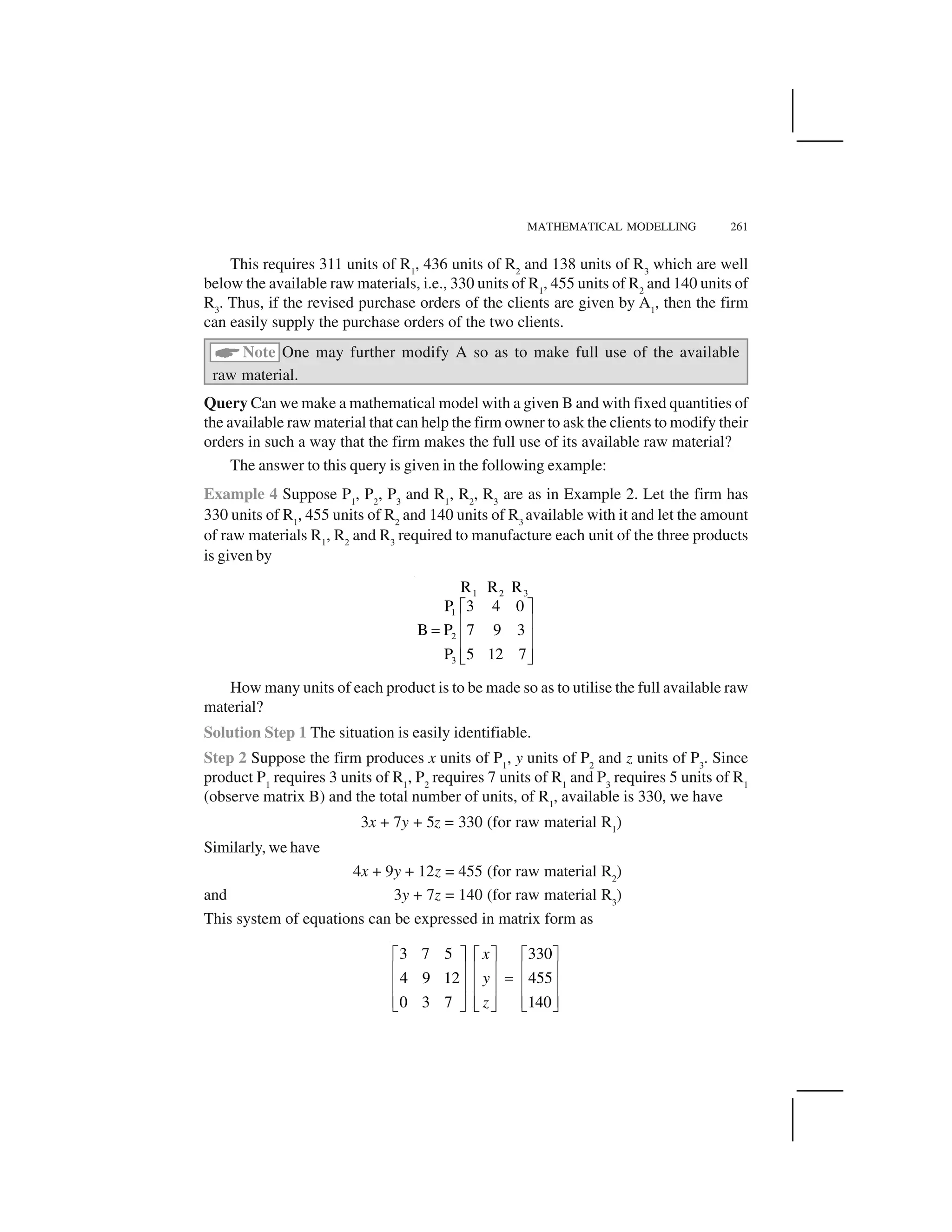
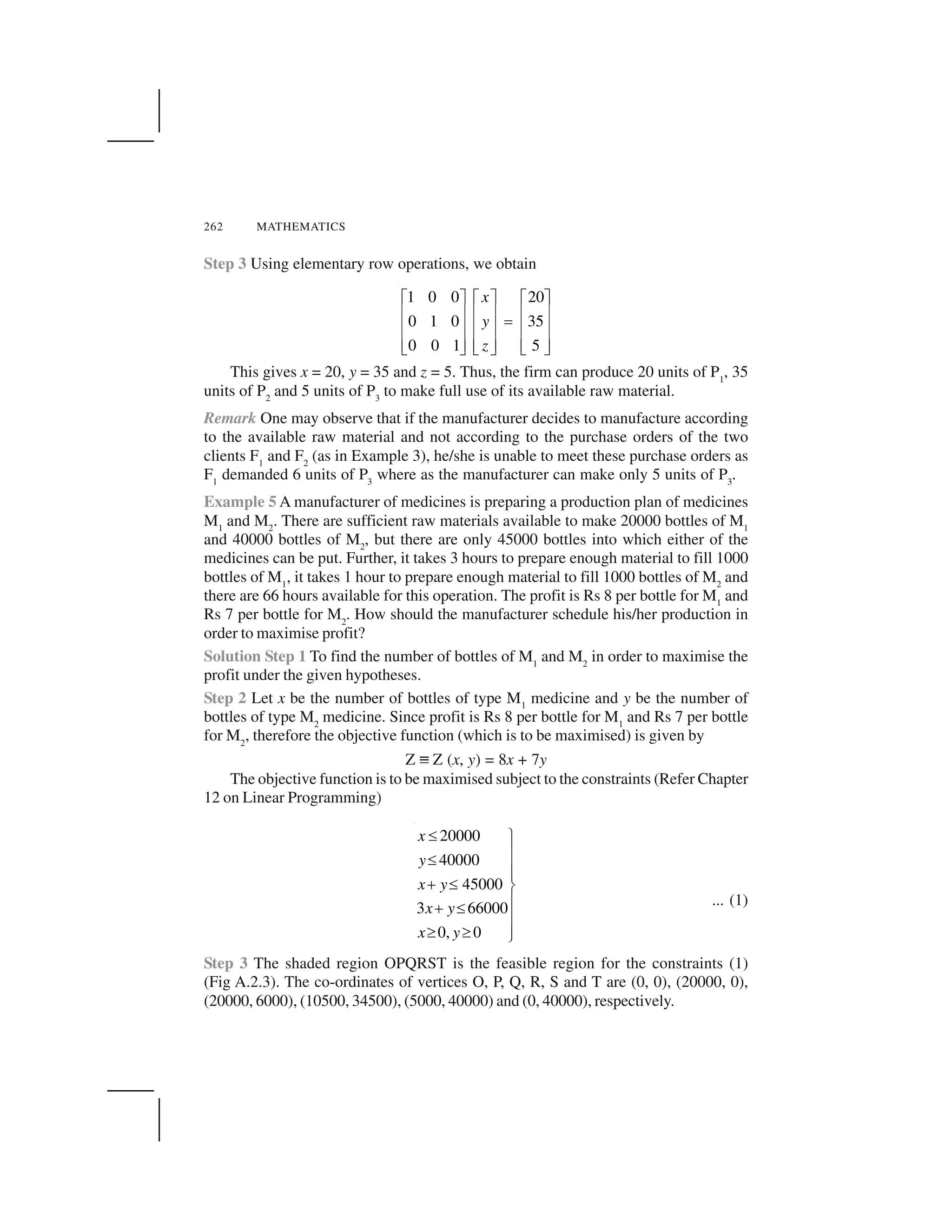
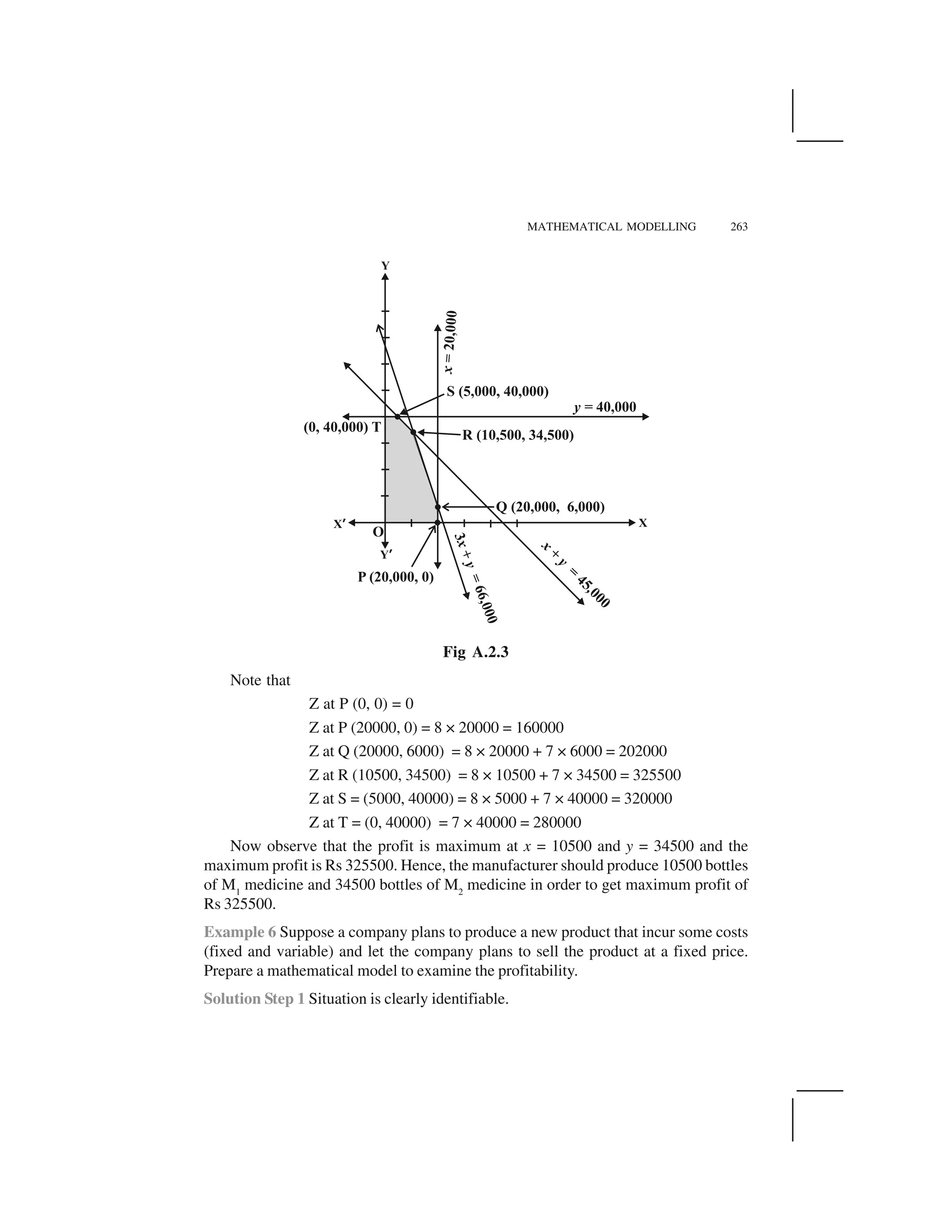


![Matematika terapan week 5 [compatibility mode]](https://cdn.slidesharecdn.com/ss_thumbnails/matematikaterapanweek5compatibilitymode-141126075318-conversion-gate01-thumbnail.jpg?width=640&height=640&fit=bounds)


