Music 100.rtfd1#[email protected]!#button.gif__MACOSX.docx

Music 100%.rtfd/1__#[email protected]%!#__button.gif
__MACOSX/Music
100%.rtfd/._1__#[email protected]%!#__button.gif
Music 100%.rtfd/1__#[email protected]%!#__icon.png
__MACOSX/Music
100%.rtfd/._1__#[email protected]%!#__icon.png
Music 100%.rtfd/2__#[email protected]%!#__button.gif
__MACOSX/Music
100%.rtfd/._2__#[email protected]%!#__button.gif
Music 100%.rtfd/button.gif
__MACOSX/Music 100%.rtfd/._button.gif
Music 100%.rtfd/downtick.png
__MACOSX/Music 100%.rtfd/._downtick.png
Music 100%.rtfd/icon.png
__MACOSX/Music 100%.rtfd/._icon.png
Music 100%.rtfd/record.gif
__MACOSX/Music 100%.rtfd/._record.gif
Music 100%.rtfd/TXT.rtf
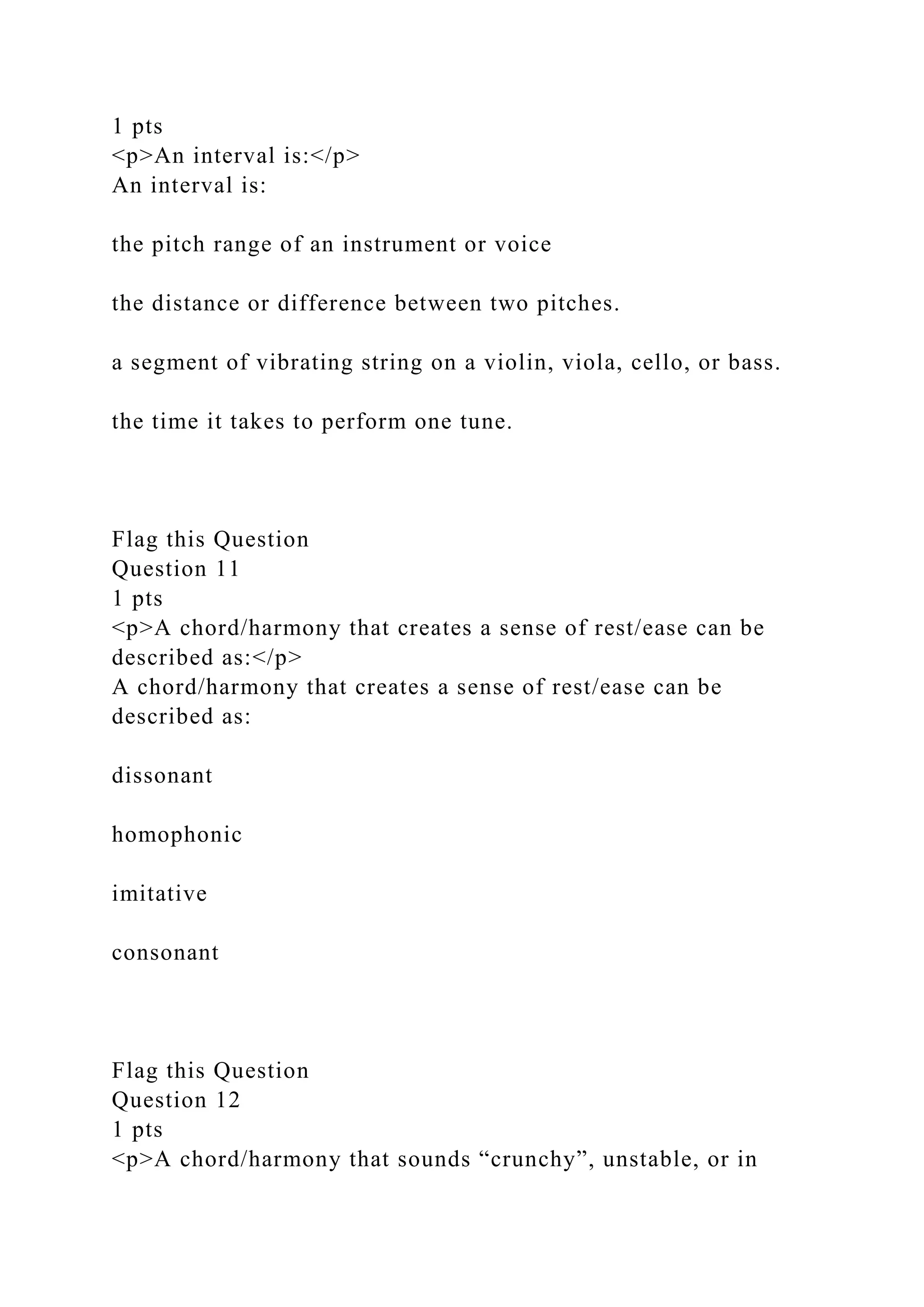
Match the vocabulary word and it's definition.

Dynamic
[ Choose ]
Pitches organized with rhythm as a recognizable unit
that has a beginning, middle and end. Like words in a sentence.
The largest structure, it is created by repetition and
contrast of the smaller Structures.
The time aspect of music, the length of the sound being
made.
How loud or soft the sound is.
More than one pitch sounding at the same time.
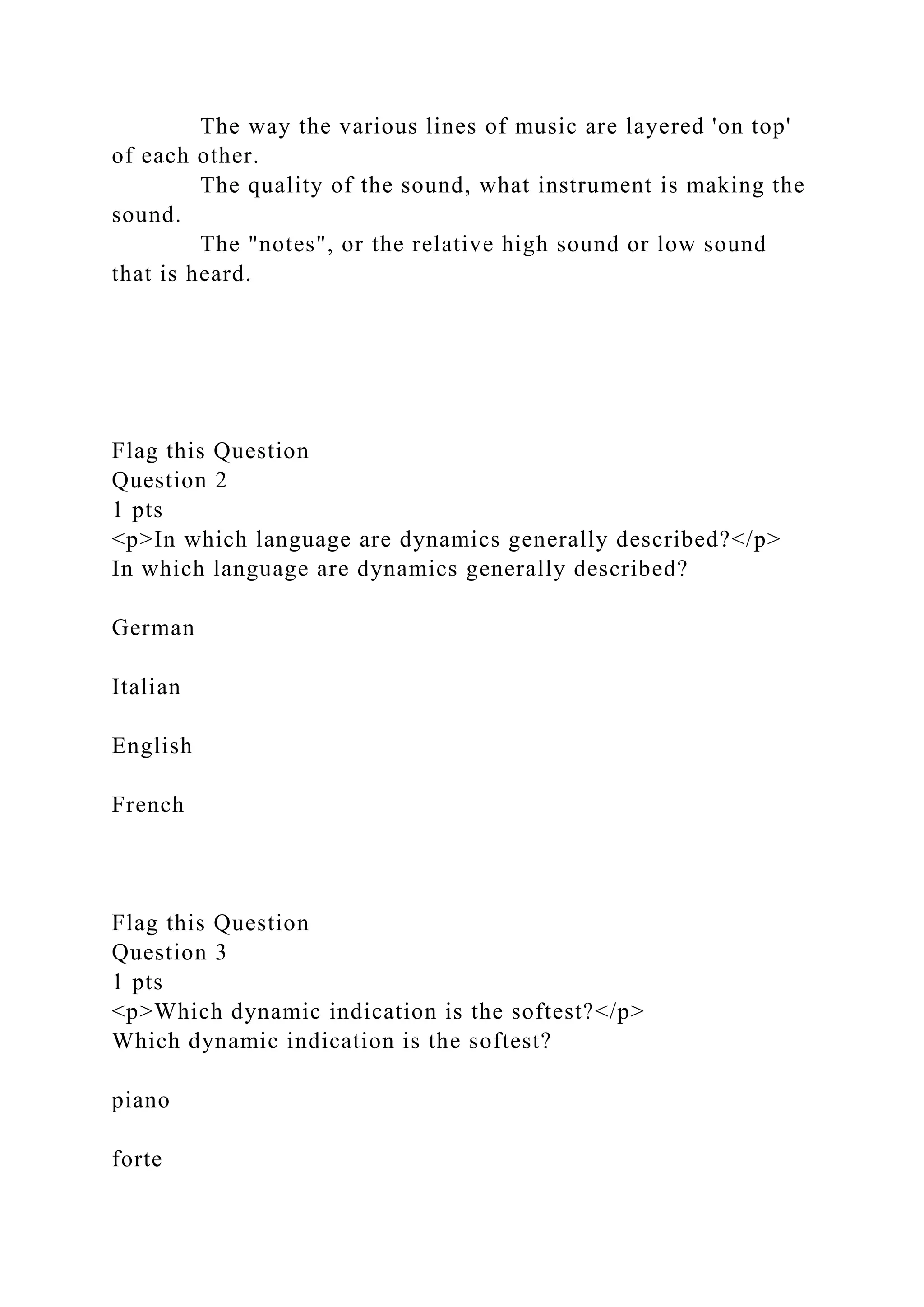
The way the various lines of music are layered 'on top'
of each other.
The quality of the sound, what instrument is making the
sound.
The "notes", or the relative high sound or low sound
that is heard.
Pitch
[ Choose ]
made.
of each other.
sound.
that is heard.

Tone Color/Timber
[ Choose ]
made.
of each other.
sound.
that is heard.
Melody
[ Choose ]
made.
of each other.
sound.

that is heard.
Rhythm
[ Choose ]
made.
of each other.
sound.
that is heard.
Harmony
[ Choose ]
made.
of each other.

sound.
that is heard.
Texture
[ Choose ]
made.
of each other.
sound.
that is heard.
Form
[ Choose ]
made.

of each other.
sound.
that is heard.
Flag this Question
Question 2
1 pts
In which language are dynamics generally described?
In which language are dynamics generally described?
German
Italian
English
French
Flag this Question
Question 3
1 pts
Which dynamic indication is the softest?
Which dynamic indication is the softest?
piano
forte

subito
mezzo piano
Flag this Question
Question 4
1 pts
What is the musical term for “loud”?
What is the musical term for “loud”?
major
sforzando
piano
forte
Flag this Question
Question 5
1 pts
What is the musical term for “suddenly”?
What is the musical term for “suddenly”?
subito
sforzando
forte
piano

Flag this Question
Question 6
1 pts
Which term indicates a gradual increase in dynamic
level?
Which term indicates a gradual increase in dynamic level?
decrescendo
piano
crescendo
subito
Flag this Question
Question 7
1 pts
Which of these words does not describe tone color? 
 
Which of these words does not describe tone color?
lush
bright
fast
brassy

Flag this Question
Question 8
1 pts
Organizing beats into predictable repeated units called:
Organizing beats into predictable repeated units called:
an accent
meter
beat
rhythm
Flag this Question
Question 9
1 pts
Tempo is the term for the:
Tempo is the term for the:
number of beats per measure.
arrangement of short and long notes.
arrangement of rhythms over the meter.
the speed of the beat.
Flag this Question
Question 10

1 pts
An interval is:
An interval is:
the pitch range of an instrument or voice
the distance or difference between two pitches.
a segment of vibrating string on a violin, viola, cello, or bass.
the time it takes to perform one tune.
Flag this Question
Question 11
1 pts
A chord/harmony that creates a sense of rest/ease can be
described as:
A chord/harmony that creates a sense of rest/ease can be
described as:
dissonant
homophonic
imitative
consonant
Flag this Question
Question 12
1 pts
A chord/harmony that sounds “crunchy”, unstable, or in

need of resolution is called:
A chord/harmony that sounds “crunchy”, unstable, or in need of
resolution is called:
dissonant.
a motive.
polyphonic
consonant
Flag this Question
Question 13
1 pts
The texture of a single melody played without
accompaniment is:
The texture of a single melody played without accompaniment
is:
monophony
homophony
polyphony
imitative counterpoint
Flag this Question
Question 14
3 pts
Define Genre in detail:

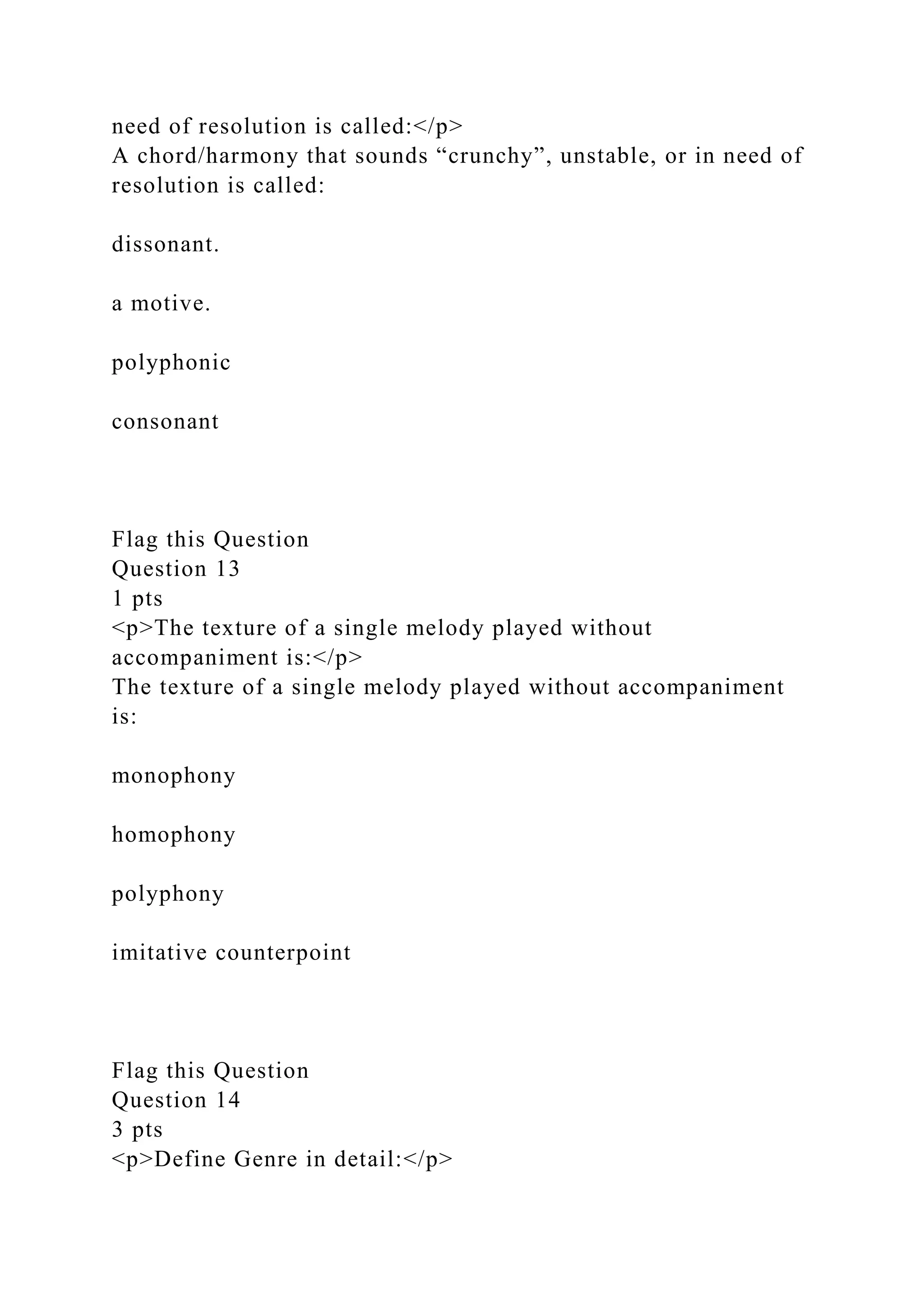
Define Genre in detail:
Keyboard Shortcuts
button.gif ¬1__#[email protected]%!#__button.gif
¬2__#[email protected]%!#__button.gif ¬icon.png
¬1__#[email protected]%!#__icon.png ¬downtick.png
¬record.gif ¬Font SizeParagraph
Flag this Question
Question 15
3 pts
Define Era and explain how they are ‘created’
Define Era and explain how they are ‘created’
__MACOSX/Music 100%.rtfd/._TXT.rtf
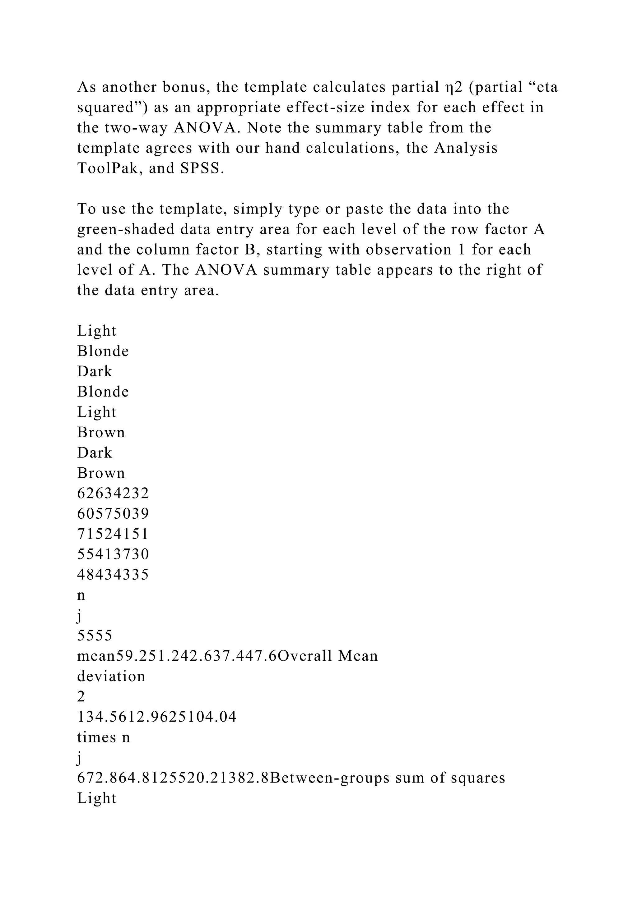
One-Way and Two-Way ANOVA in Excel
Larry A. Pace, Ph.D.
Let us learn to conduct and interpret a one-way ANOVA and a
two-way ANOVA for a balanced factorial design in Excel, using
the Analysis ToolPak. We will perform the calculations by use
of formulas and compare the results with those from the
ToolPak and from SPSS. As a bonus, the reader will have access
to a worksheet template for the two-way ANOVA that automates
all the calculations required for Module 6, Assignment 2.One-
way ANOVA
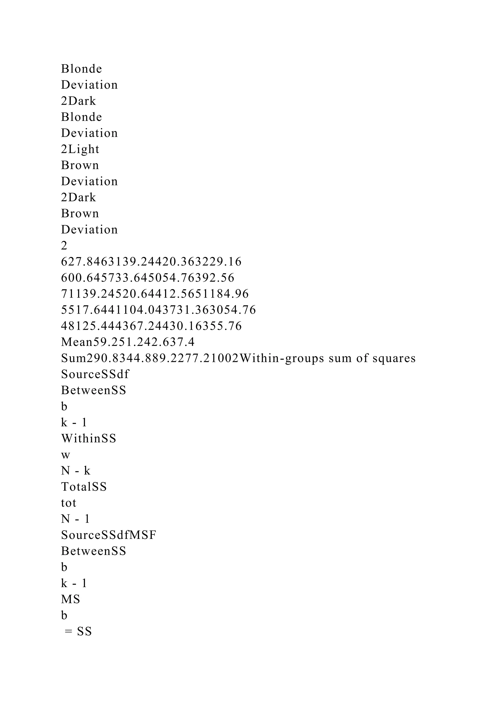
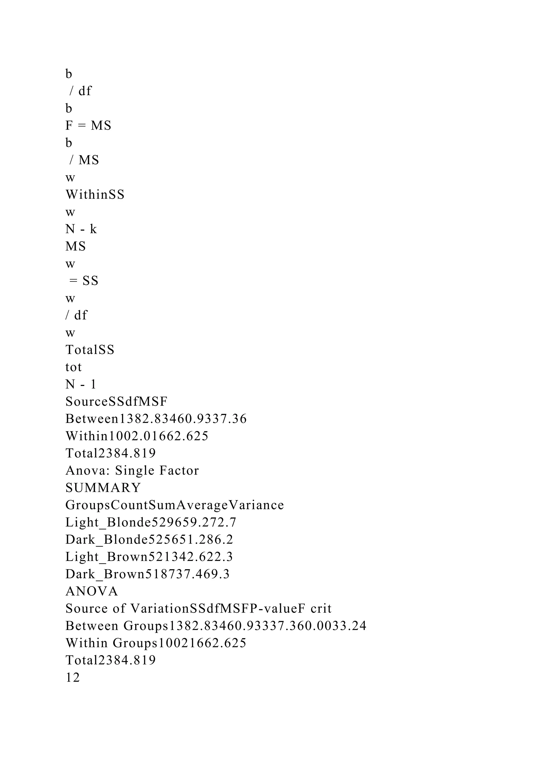
The analysis of variance (ANOVA) allows us to compare three
or more means simultaneously, while controlling for the overall
probability of making a Type I error (rejecting a true null
hypothesis). Researchers developed a test to measure
participants’ pain thresholds. The researchers sought to

determine whether participants’ hair color had any influence on
her pain tolerance. Twenty participants were divided into four
equal-sized groups based on natural, and their pain tolerance
was measured. The dependent variable is the pain tolerance
score, and the independent variable (or factor) is the
participant’s hair color. In ANOVA, the independent variable is
the “grouping” variable that determines group membership for
each participant. Consider the following hypothetical pain
threshold data. Higher scores indicate higher pain tolerance.
Hair Color
Light Blonde
Dark Blonde
Light Brown
Dark Brown
62
63
42
32
60
57
50
39
71
52
41
51
55
41
37
30
48
43
43
35
The null hypothesis is that the population means are equal. The

alternative hypothesis is that at least one pair of means is
unequal. We can symbolize these hypotheses as follows:
H0: µ1 = µ2 = µ3 = µ4
H1: µ1 ≠ µ2 ≠ µ3 ≠ µ4
Partitioning the Total Sum of Squares
Analysis of variance partitions or “analyzes” the total variation
into between-groups variation (based on differences between the
means of the groups) and within-groups variation (based on
differences between the individual values and the mean of the
group to which that value belongs). Symbolically:
SStot = SSb + SSw
The total sum of squares, SStot is found (by definition) as
follows. Find the overall mean of all observations, ignoring the
group membership. Let us use x “double bar” to represent the
mean of all the observations, which is sometimes called the
“grand mean.”
We have 4 groups with 5 observations each, so we have 20 total
observations. Treating all 20 observations as a single dataset,
the mean is 47.6. To find the total sum of squares, subtract the
mean from every value, square this deviation score, and then
add up all the squared deviations:
and thus,
Although this is instructive, it is quite laborious and is not the
way we would compute the sum of squares by hand. Instead, we
would use a computing form that is algebraically equivalent to
our definitional form, but requires us simply to square and sum
our raw score values, rather than to find individual deviation
scores.
The sum of squares total can be found by summing all the
squared values, and subtracting from that total the sum of the
individual values squared and divided by N, the total number of

observations. This formula gives us exactly the same value as
the definitional formula. See the Excel screen shot below. The
selected cell, C16, contains the formula for squaring the sum of
the x values and dividing the square by N. When we subtract
that value from the sum of the squares of all the scores, the
remainder is the total sum of squares.
Once you understand what the total sum of squares represents,
you can easily use technology to find it without having to do
repetitive calculations. Use the DEVSQ function in Excel to
find the sum of squares from raw data. See the formula in the
Formula Bar and the resulting value in cell E7. To get this
answer, simply click in cell E7 and type the formula exactly as
you see it in the Formula Bar.
Now that we have the total sum of squares, let us partition it
into two different sources. The between-groups sum of squares
is based only on the differences between the group means and
the overall mean. We weight the group mean by the number of
observations in the group (because that is the number of
observations that went into calculating the mean) and multiply
the squared deviation from the overall mean for that group by
the group size. Add this up across all groups, and you have the
between-groups sum of squares. It is easier to show this by use
of a formula than to write it in words. Let us call the number of
groups k. In our case, k = 4. Further, let us say there are n1 +
n1+…+nk = N total observations. In our case, we have 5 + 5 + 5
+ 5 = 20 observations. The definitional formula of the between-
groups sum of squares is:
For our pain threshold data, we would have the following
results.
The within-groups sum of squares is found by summing the
squared deviations from the mean for each score in that group,

and then summing across groups. The double summation just
says find the squared deviations for each group and then add
them all up across the groups.
The table below shows the calculation of the within-groups sum
of squares.
Because of the additivity principle of variance, we could just as
easily have found the within-groups sum of squares by simple
subtraction:
SStot = SSb + SSw
SStot - SSb = SSw
2384.8 – 1382.8 = 1002
Partitioning the Degrees of Freedom
You will recall the concept of degrees of freedom (number of
values free to vary) from your module on t tests. In ANOVA, we
partition the total degrees of freedom in a fashion similar to the
way we partition the total sum of squares. Remember the basic
“n minus one” definition for degrees of freedom. If you have 20
total observations, you have 19 total degrees of freedom. If you
have 4 groups, you have 3 degrees of freedom between groups.
If you have 5 observations in a group, you have 4 degrees of
freedom in that group. Using the same symbols we have already
discussed, we have N – 1 total degrees of freedom. We have k –
1 degrees of freedom between groups, and we have N – k
degrees of freedom within groups. The table below shows the
partition of the total sum of squares and of the degrees of
freedom.
Mean Squares and the F Ratio
Dividing a sum of squares by its degrees of freedom produces a
“mean square” or MS. A mean square is a variance estimate,
and we calculate an F ratio by dividing two variance estimates.
The MSb is the variance due to differences between the means

of the groups, and the MSw is the variance due to differences
within the groups. By calculating an F ratio, we determine how
large the between-group variance is, relative to the within-group
variance. Let us build this additional information into our
ANOVA summary table.
If the two variance estimates were equal, the F ratio would be 1.
As the F ratio increases, the amount of variation due to “real
differences” between the groups increases. As with a t test, we
can find the probability of obtaining an F ratio as large as or
larger than the one we obtained if the null hypothesis of no
differences is true. We will compare the p value we obtain to
the alpha level for our test, which we usually set to .05. If our p
value is lower than .05, we reject the null hypothesis. If the p
value is greater than .05, we retain the null hypothesis.
Using our current example, let us complete our ANOVA
summary table.
To test the significance of an F ratio of 7.36 with 3 and 16
degrees of freedom, we can use Excel’s FDIST function. The
function takes three arguments, which are the value of F, the
degrees of freedom for the numerator term, and the degrees of
freedom for the denominator term. We see that our F ratio has a
p value much lower than .05, so our decision is to reject the null
hypothesis.
Writing the Results of the ANOVA in APA Format
In our APA summary statement, we do not say we rejected the
null hypothesis, but instead that the results are statistically
significant, which is another way of saying the same thing. An
APA-style conclusion for our analysis might be as follows:
A one-way ANOVA revealed that there are significant
differences in pain thresholds among women of different hair
color, F(3, 16) = 7.36, p = .003.

Using the Analysis ToolPak for a One-Way ANOVA
First, ensure you have the Analysis ToolPak installed. If you do,
there will be a Data Analysis option in the Analysis group of
the Data ribbon.
If you do not see this option, click on the Office Button, then
Excel Options > Add-ins > Manage Excel Add-ins > Go. In the
resulting dialog box, check the box in front of “Analysis
ToolPak,” and click OK.
To conduct the one-way ANOVA, first make sure your data are
in a worksheet arranged as follows. The labels and borders are
purely optional. Because we will use labels, we must inform
Excel of that fact.
Click on Data > Analysis > Data Analysis. In the Data Analysis
dialog box, scroll to Anova: Single Factor, and then click OK.
Enter the input range by dragging through the entire dataset,
including the labels. Check “Labels in First Row,” and then
click OK. The results of the ANOVA will appear in a new
worksheet.
I have formatted the table’s number formatting to be consistent
with APA style.
Note the Analysis ToolPak produces the same values as we did
with our manual calculations. An ANOVA summary table from
SPSS is shown below. SPSS produces the same results as the
Analysis ToolPak. Note SPSS uses the label “Sig.” for
significance as a label for the p value.
Going Further: Effect Size
Because our ANOVA is significant, we might ask the very
reasonable question, “How big is the effect?” One very good

way to answer this question is to calculate an effect size index
known as η2 (“eta squared”). This index tells us what
proportion of the total variation in the dependent variable can
be explained (or “accounted for”) by knowing the independent
variable. In our case, we would ask what proportion of variation
in pain tolerance can be explained by knowing a woman’s hair
color. We calculate η2 by dividing the between-groups sum of
squares by the total sum of squares. In our example, 1382.8 /
2384.8 = .58, so a substantial amount of the variation is
explained.
Going Further: Post Hoc Comparisons
After a significant ANOVA, we know that at least one pair of
means is different, but we do not yet know which pair or pairs
are significantly different. We want to control the probability of
making a Type I error, so we want to use a post hoc comparison
procedure that holds the overall or “experimentwise” error rate
to no more than our original alpha level. Two very popular post
hoc procedures are the Tukey HSD (for honestly significant
difference) procedure and Bonferroni-corrected comparisons.
The Tukey HSD test uses a distribution called the “studentized
range statistic,” while the Bonferroni procedure uses the t
distribution with which you are already familiar. For that
reason, we will illustrate the Bonferroni procedure. We will
calculate a new value of t using the following formula:
We find the difference between two of the means, and divide
that by a standard error term based on all the groups rather than
just the two groups in consideration. We weight the error term
by the sizes of the two groups, but for the t test, we use the
within-groups degrees of freedom instead of n1 + n2 – 2 as we
would in an independent-samples t test. Then, to make the
Bonferroni correction, we divide the alpha level for the overall
ANOVA by the number of possible pairings of means. Because

we have 4 groups, there are 6 possible pairings:
Thus we would have α / 6 = .05 / 6 = .0083 as the required level
of significance to reject the null hypothesis that the two means
in question are different. If we wanted to do this in reverse
using the p value approach, we could find the p value for our t
test with dfw, and then multiply that p value by the number of
possible pairings. Let us work out one example. We will
compare the means of light blondes and dark brunettes:
Using Excel’s TDIST function, we find this value of t has a
two-tailed p value of .0005 with 16 degrees of freedom.
This is lower than .0083, and we can reject the null hypothesis
and conclude that light blondes have a significantly higher pain
tolerance threshold than dark brunettes. If we use the p value
approach, we can multiply .0005 by 6 to find the actual p value
to be approximately .003. Rather than doing all these corrected t
tests by hand, we might use a technology such as SPSS to
perform all the pairwise comparisons. Note in the SPSS output
that the mean difference, the standard error term, and the p
value for the comparison of light blondes and dark brunettes all
agree with our calculations above.
The Two-Way ANOVA
In the one-way ANOVA, we have a single factor. In our
example, the factor is the grouping variable hair color. In the
two-way ANOVA, we have two factors. For example, we might
have one factor that as before is hair color and another factor
that is sex. In our first example, we had females only. What if
we repeated our experiment, but added males? In the two-way
ANOVA, we can determine whether there are sex differences,
whether there are differences by hair color, and whether there is
an interaction between sex and hair color. We will consider only
the simplest of cases, a balanced factorial design with equal
numbers of observations in every cell of the data table. Assume
we have the following data:

Partitioning the Total Sum of Squares in Two-Way ANOVA
In the two-way ANOVA, we can define and calculate the total
sum of squares in an identical fashion to the one-way ANOVA.
We now have a sum of squares for A, the row factor, a sum of
squares for B, the column factor, a sum of squares for the
interaction between the A and B factors, and a residual (for
what is left over) sum of squares that we will use as our error
term. Our partition is
SStot = SSA + SSB + SSAB + SSerr
Simply calculate the overall or grand mean, subtract that mean
from every individual observation, square the deviation score,
and sum the squared deviations.
Let us change our symbols slightly to accommodate the present
case. Let C represent the number of columns (our B factor), and
R (for rows) represent the number of levels of our A factor. Let
G (for group) represent the number of observations per cell.
Then we have N = C × R × G. In our example there are 2 levels
of A, 4 levels of B, and 5 observations per cell, so N = 2 × 4 × 5
= 40. Thus we have 40 – 1 = 39 total degrees of freedom.
We calculate the sum of squares for cells as the sum of the
squared deviations of the individual cell means from the overall
mean multiplied by the number of observations per group. This
is the overall “between groups” variation, which we partition
further into SSA, SSB and SSAB.
Use the marginal means for the row factor A, ignoring the
column factor B, to calculate the sum of squares for A:
with R – 1 degrees of freedom. In a similar fashion, the sum of
squares for factor B, ignoring the row factor A, is
with G – 1 degrees of freedom. Subtracting the sum of squares
for A and B from the sum of squares for cells gives the sum of

squares for the interaction of A and B,
with (R – 1) × (C – 1) degrees of freedom. Finally, we can also
find the error sum of squares by subtraction:
with RC × (G – 1) degrees of freedom. We calculate the mean
square for each term by dividing the sum of squares by the
respective degrees of freedom and then calculate the F ratio for
each effect by dividing the mean square for that effect by the
error mean square. Because these calculations are laborious, we
will usually allow technology to do them for us, though the
learner may benefit from working a small example by hand. Let
us do the calculations for our revised example.
We can use the DEVSQ function in Excel to find the total
degrees of freedom from the raw data, as we did in our one-way
ANOVA.
Below is a table of the cell and marginal means for our dataset.
Let us use our A and B labeling to make sure we understand the
row and column factors.
We can use this information to help us calculate the various
sums of squares. The sum of squares for cells is the number of
observations per cell multiplied by the deviations for each cell
from the overall mean of all observations. There are 5
observations per cell, so the cell sum of squares is
The cell sum of squares is an intermediate step for finding the
AB interaction sum of squares, so we will now calculate the
sum of squares for A, our row factor. We will multiply the
number of columns by the number of observations per cell, and
multiply this by the squared deviations of the row marginal
means from the overall mean.
Similarly, we find the column sum of squares by multiplying the

number of rows by the number of observations per cell, and
multiply that by the squared deviations of the column marginal
means from the overall mean.
We can now find the AB interaction sum of squares by
subtraction:
We can also find the error sum of squares by subtraction:
In the two-way ANOVA we will have the following ANOVA
summary table with the degrees of freedom as shown. Note
there are three F ratios, one for the A main effect, one for the B
main effect, and one for the AB interaction. Each F ratio uses
the same error term, which is the error mean square.
Using the information from our current example, we have the
following summary table:
Note there is a significant main effect for sex (Factor A), and a
significant main effect for hair color (Factor B). The interaction
of hair color and sex is not significant. We might write our
results as follows:
A two-way ANOVA revealed a significant main effect for sex,
F(1, 32) = 142.47, p < .001, and a significant main effect for
hair color, F(3, 32) = 13.01, p < .001. There was no interaction
between sex and hair color, F(3, 32) = 0.44, p = .723.
Doing the Two-Way ANOVA in the Analysis ToolPak
Make sure the Analysis ToolPak is installed. Input the data as
shown below. I will use A and B to reinforce the concept of row
and column factors as discussed above.
Select Data > Analysis > Data Analysis. In the Data Analysis
dialog box, scroll to Anova: Two-factor With Replication.

Click OK, and in the resulting dialog, drag through the entire
range of data, including the labels. The “rows per sample”
indicate the number of observations per cell.
Click OK. Excel conducts the ANOVA procedure and places the
results in a new worksheet (shown after cell formatting). The
ANOVA summary table appears below. Excel calls the row
factor “Samples,” and the column factor “Columns.” Apart from
this labeling difference, the results are identical to those we
calculated with the definitional formulas.
Going Further: Two-Way ANOVA in SPSS with Bonferroni
Comparisons
The two-way ANOVA in SPSS produces exactly the same
results as the Analysis ToolPak.
Because there are only two levels of A, there is no need for
additional comparisons for that factor. But there are four levels
of B (hair color), so we can compare the means for the levels of
B using Bonferroni comparisons. We see again that regardless
of sex, people with light blond hair have higher pain tolerance
than people with light and dark brunette hair. Further, we see
that people with dark blonde hair have higher pain tolerance
than those with dark brunette hair.
Bonus: A Two-Way ANOVA Worksheet Template
I have created a two-way ANOVA template in Excel. This
template requires only that the user type or paste the data in the
appropriate cells. The template is programmed to have as many
as 10 observations per cell, and will work with up to five levels
of a row factor A and 10 levels of a column factor B. The
current data correctly entered into the template are as follows:

As another bonus, the template calculates partial η2 (partial “eta
squared”) as an appropriate effect-size index for each effect in
the two-way ANOVA. Note the summary table from the
template agrees with our hand calculations, the Analysis
ToolPak, and SPSS.
To use the template, simply type or paste the data into the
green-shaded data entry area for each level of the row factor A
and the column factor B, starting with observation 1 for each
level of A. The ANOVA summary table appears to the right of
the data entry area.
Light
Blonde
Dark
Blonde
Light
Brown
Dark
Brown
62634232
60575039
71524151
55413730
48434335
n
j
5555
mean59.251.242.637.447.6Overall Mean
deviation
2
134.5612.9625104.04
times n
j
672.864.8125520.21382.8Between-groups sum of squares
Light

Blonde
Deviation
2Dark
Blonde
Deviation
2Light
Brown
Deviation
2Dark
Brown
Deviation
2
627.8463139.24420.363229.16
600.645733.645054.76392.56
71139.24520.64412.5651184.96
5517.6441104.043731.363054.76
48125.444367.24430.16355.76
Mean59.251.242.637.4
Sum290.8344.889.2277.21002Within-groups sum of squares
SourceSSdf
BetweenSS
b
k - 1
WithinSS
w
N - k
TotalSS
tot
N - 1
SourceSSdfMSF
BetweenSS
b
k - 1
MS
b
= SS

b
/ df
b
F = MS
b
/ MS
w
WithinSS
w
N - k
MS
w
= SS
w
/ df
w
TotalSS
tot
N - 1
SourceSSdfMSF
Between1382.83460.9337.36
Within1002.01662.625
Total2384.819
Anova: Single Factor
SUMMARY
GroupsCountSumAverageVariance
Light_Blonde529659.272.7
Dark_Blonde525651.286.2
Light_Brown521342.622.3
Dark_Brown518737.469.3
ANOVA
Source of VariationSSdfMSFP-valueF crit
Between Groups1382.83460.93337.360.0033.24
Within Groups10021662.625
Total2384.819
12

w
12
11
xx
t
MS
nn
-
=
æö
+
ç÷
èø
(
)
1
43
6
22
kk
´-
´
==
(
)
12
w
12
59.237.421.8
62.6250.40
11
11
62.625
55
21.821.8
4.356

5.005
25.05
xx
t
MS
nn
-
-
===
æöæö
+
+
ç÷
ç÷
èø
èø
===
Light BlondeDark BlondeLight BrownDark Brown
Female
62634232
60575039
71524151
55413730
48434335
Male
89767275
90868264
79786969
72847859
84696763
2
cells
11
()
RC
ij

ij
SSGXX
==
=-
åå
2
A
1
()
R
i
i
SSCGXX
=
=-
å
2
B
1
()
C
j
j
SSRGXX
=
=-
å
ABcellsAB
SSSSSSSS
=--
errtotcells
SSSSSS
=-
B1B2B3B4Row Mean
A159.251.242.637.447.6
A282.878.673.66675.25

Col. Mean7164.958.151.761.425
(
)
2222
2
2222
11
(59.261.425)(51.261.425)(42.661.425)(37.
461.425)
55
(82.861.425))(78.661.425)(73.661.425)(66
61.425)
9810.575
RC
ij
ij
XX
==
æö
-+-+-+-
´-=
ç÷
ç÷
+-+-+-+-
èø
=
åå
ABcellsAB
9810.5757645.2252093.87571.475
SSSSSSSS
=--
=--=
errtotcells
11527.7759810.5751717.2
SSSSSS
=-=-=

SourceSSdfMSF
ASS
A
R-1
MS
A
= SS
A
/df
A
MS
A
/MS
err
BSS
B
C-1
MS
B
= SS
B
/df
B
MS
B
/MS
err
ABSS
AB
(R-1)(C-1)
MS
AB
=SS
AB
/df
AB

MS
AB
/MS
err
ErrorSS
err
RC(G-1)
MS
err
=SS
err
/df
err
TotalSS
tot
N-1
SourceSSdfMSFP-value
A7645.22517645.225142.470.000
B2093.8753697.958333313.010.000
AB71.475323.8250.440.723
Error1717.23253.6625
Total11527.77539
(62-47.6)
2
(63-47.6)
2
(42-47.6)
2
(32-47.6)
2
(60-47.6)
2
(57-47.6)
2
(50-47.6)

2
(39-47.6)
2
(71-47.6)
2
(52-47.6)
2
(41-47.6)
2
(51-47.6)
2
(55-47.6)
2
(41-47.6)
2
(37-47.6)
2
(30-47.6)
2
(48-47.6)
2
(43-47.6)
2
(43-47.6)
2
(35-47.6)
2
ANOVA
Source of Variation
SS
df
MS
F
P-value
F crit
Sample

7645.225
1
7645.225
142.47
0.000
4.15
Columns
2093.875
3
697.9583333
13.01
0.000
2.90
Interaction
71.475
3
23.825
0.44
0.723
2.90
Within
1717.2
32
53.6625
Total
11527.775
39
Source of VariationSSdfMSFpPartial η
2
A (Row Factor)7645.22517645.225142.47.000.817
B (Column Factor)2093.8753697.95813.01.000.549
A x B Interaction71.475323.8250.44.723.040
Error1717.2003253.663
Total11527.77539
207.36237.1631.36243.36

153.7688.365.7673.96
547.5619.3643.5611.56
54.7643.56112.36309.76
0.1621.1621.16158.76
Sum963.6409.6214.2797.42384.8Total Sum of Squares

Music 100.rtfd1__#[email protected]!#__button.gif__MACOSX.docx

More Related Content

Similar to Music 100.rtfd1__#[email protected]!#__button.gif__MACOSX.docx

More from rosemarybdodson23141

Recently uploaded