This document discusses multiple linear regression, explaining the model used to analyze the impact of multiple explanatory variables on a response variable. It covers aspects such as regression coefficients, the use of categorical explanatory variables through dummy coding, and the interpretation of results in the context of a specific example involving childhood respiratory health. The document emphasizes the need for statistical software to calculate multiple regression statistics and details how to interpret coefficients, including their confidence intervals.

1. Basic Biostat 15: Multiple Linear Regression 1
Chapter 15:
Multiple Linear Regression

2. Basic Biostat 15: Multiple Linear Regression 2
In Chapter 15:
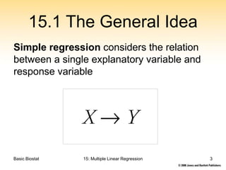
15.1 The General Idea
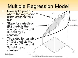
15.2 The Multiple Regression Model
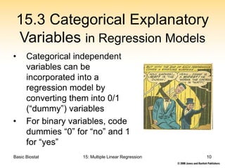
15.3 Categorical Explanatory Variables
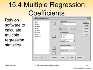
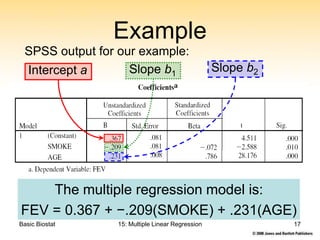
15.4 Regression Coefficients
[15.5 ANOVA for Multiple Linear Regression]
[15.6 Examining Conditions]
[Not covered in recorded presentation]

3. Basic Biostat 15: Multiple Linear Regression 3
15.1 The General Idea
Simple regression considers the relation
between a single explanatory variable and
response variable

4. Basic Biostat 15: Multiple Linear Regression 4
The General Idea
Multiple regression simultaneously considers the
influence of multiple explanatory variables on a
response variable Y
The intent is to look at
the independent effect
of each variable while
“adjusting out” the
influence of potential
confounders

5. Basic Biostat 15: Multiple Linear Regression 5
Regression Modeling
• A simple regression
model (one independent
variable) fits a regression
line in 2-dimensional
space
• A multiple regression
model with two
explanatory variables fits
a regression plane in 3-
dimensional space

6. Basic Biostat 15: Multiple Linear Regression 6
Simple Regression Model
Regression coefficients are estimated by
minimizing ∑residuals2 (i.e., sum of the squared
residuals) to derive this model:
The standard error of the regression (sY|x) is
based on the squared residuals:

7. Basic Biostat 15: Multiple Linear Regression 7
Multiple Regression Model
Again, estimates for the multiple slope
coefficients are derived by minimizing ∑residuals2
to derive this multiple regression model:
Again, the standard error of the regression
is based on the ∑residuals2:

8. Basic Biostat 15: Multiple Linear Regression 8
Multiple Regression Model
• Intercept α predicts
where the regression
plane crosses the Y
axis
• Slope for variable X1
(β1) predicts the
change in Y per unit
X1 holding X2
constant
• The slope for variable
X2 (β2) predicts the
change in Y per unit
X2 holding X1
constant

9. Basic Biostat 15: Multiple Linear Regression 9
Multiple Regression Model
A multiple regression
model with k independent
variables fits a regression
“surface” in k + 1
dimensional space (cannot
be visualized)

10. Basic Biostat 15: Multiple Linear Regression 10
15.3 Categorical Explanatory
Variables in Regression Models
• Categorical independent
variables can be
incorporated into a
regression model by
converting them into 0/1
(“dummy”) variables
• For binary variables, code
dummies “0” for “no” and 1
for “yes”

11. Basic Biostat 15: Multiple Linear Regression 11
Dummy Variables, More than two
levels
For categorical variables with k categories, use k–1 dummy variables
SMOKE2 has three levels, initially coded
0 = non-smoker
1 = former smoker
2 = current smoker
Use k – 1 = 3 – 1 = 2 dummy variables to code this information like this:

12. Basic Biostat 15: Multiple Linear Regression 12
Illustrative Example
Childhood respiratory health survey.
• Binary explanatory variable (SMOKE) is
coded 0 for non-smoker and 1 for smoker
• Response variable Forced Expiratory
Volume (FEV) is measured in liters/second
• The mean FEV in nonsmokers is 2.566
• The mean FEV in smokers is 3.277

13. Basic Biostat 15: Multiple Linear Regression 13
Example, cont.
• Regress FEV on SMOKE least squares
regression line:
ŷ = 2.566 + 0.711X
• Intercept (2.566) = the mean FEV of group 0
• Slope = the mean difference in FEV
= 3.277 − 2.566 = 0.711
• tstat = 6.464 with 652 df, P ≈ 0.000 (same as
equal variance t test)
• The 95% CI for slope β is 0.495 to 0.927 (same
as the 95% CI for μ1 − μ0)

14. Basic Biostat 15: Multiple Linear Regression 14
Dummy Variable SMOKE
Regression line
passes through
group means
b = 3.277 – 2.566 = 0.711

15. Basic Biostat 15: Multiple Linear Regression 15
Smoking increases FEV?
• Children who smoked had higher mean FEV
• How can this be true given what we know
about the deleterious respiratory effects of
smoking?
• ANS: Smokers were older than the
nonsmokers
• AGE confounded the relationship between
SMOKE and FEV
• A multiple regression model can be used to
adjust for AGE in this situation

16. Basic Biostat 15: Multiple Linear Regression 16
15.4 Multiple Regression
Coefficients
Rely on
software to
calculate
multiple
regression
statistics

17. Basic Biostat 15: Multiple Linear Regression 17
Example
The multiple regression model is:
FEV = 0.367 + −.209(SMOKE) + .231(AGE)
SPSS output for our example:
Intercept a Slope b2
Slope b1

18. Basic Biostat 15: Multiple Linear Regression 18
Multiple Regression Coefficients, cont.
• The slope coefficient associated for SMOKE is
−.206, suggesting that smokers have .206 less
FEV on average compared to non-smokers
(after adjusting for age)
• The slope coefficient for AGE is .231, suggesting
that each year of age in associated with an
increase of .231 FEV units on average (after
adjusting for SMOKE)

19. Basic Biostat 15: Multiple Linear Regression 19
Coefficients
a
.367 .081 4.511 .000
-.209 .081 -.072 -2.588 .010
.231 .008 .786 28.176 .000
(Constant)
smoke
age
Model
1
B Std. Error
Unstandardized
Coefficients
Beta
Standardized
Coefficients
t Sig.
Dependent Variable: fev
a.
Inference About the Coefficients
Inferential statistics are calculated for each
regression coefficient. For example, in testing
H0: β1 = 0 (SMOKE coefficient controlling for AGE)
tstat = −2.588 and P = 0.010
df = n – k – 1 = 654 – 2 – 1 = 651

20. Basic Biostat 15: Multiple Linear Regression 20
Inference About the Coefficients
The 95% confidence interval for this slope of
SMOKE controlling for AGE is −0.368 to − 0.050.
Coefficients
a
.207 .527
-.368 -.050
.215 .247
(Constant)
smoke
age
Model
1
Lower Bound Upper Bound
95% Confidence Interval for B
Dependent Variable: fev
a.