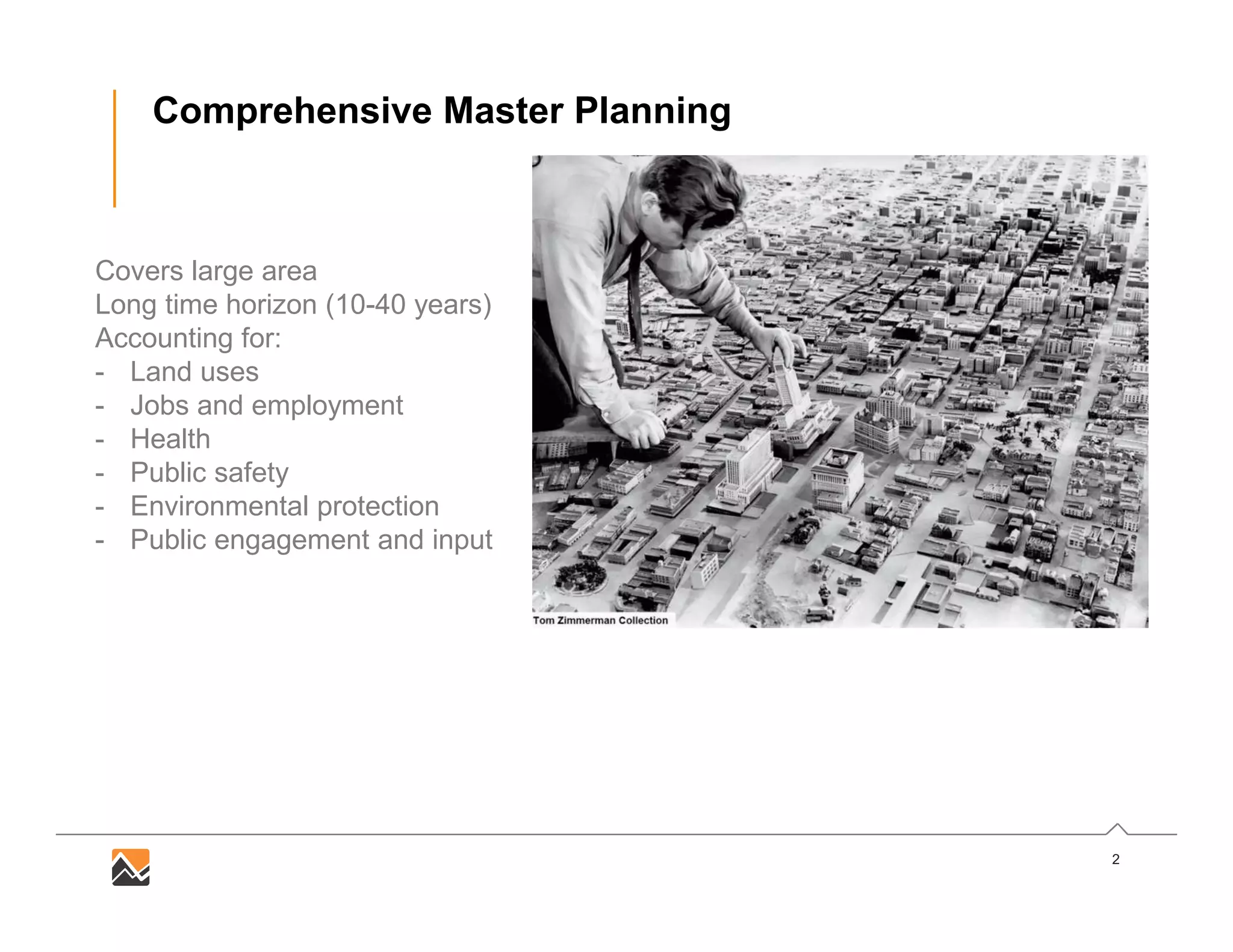
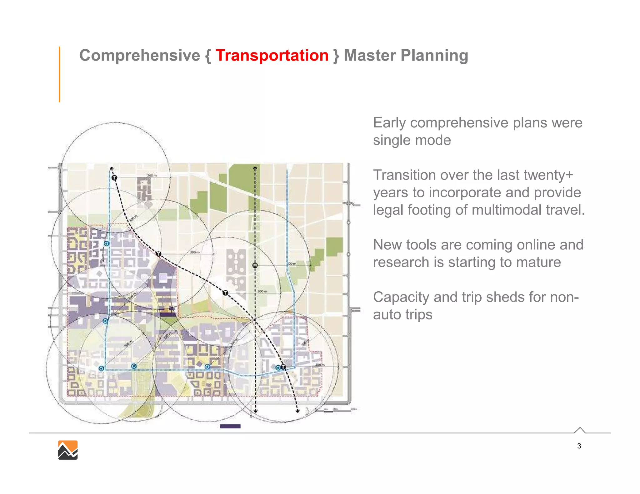
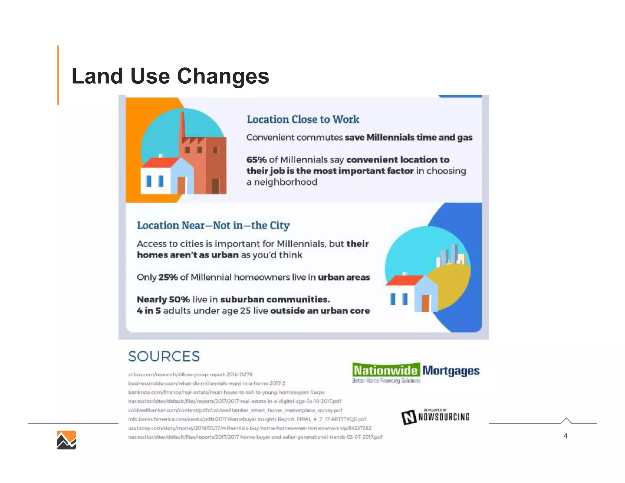
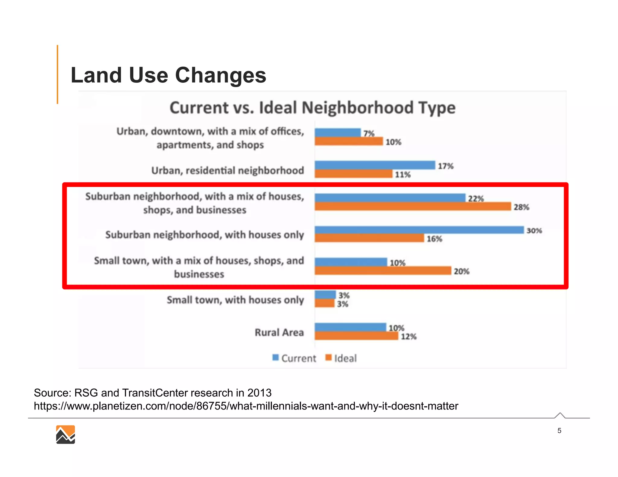
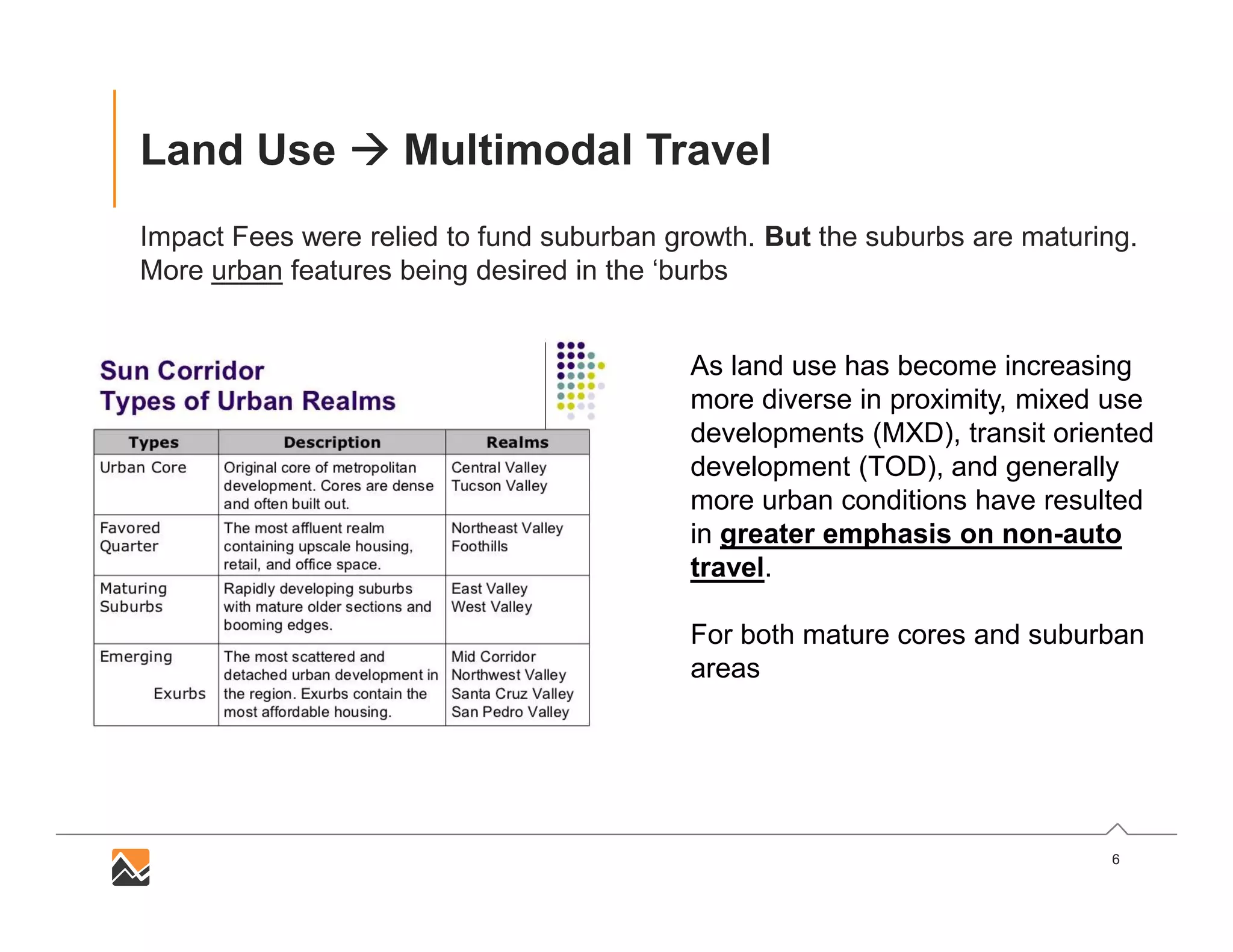
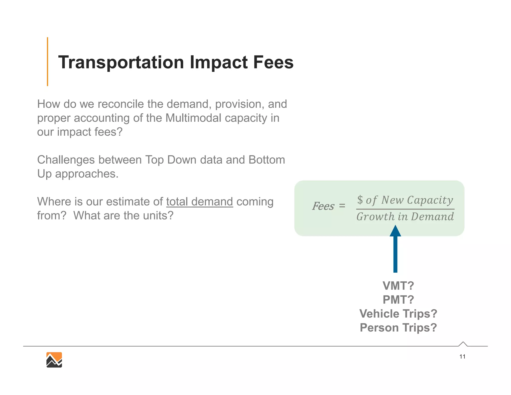
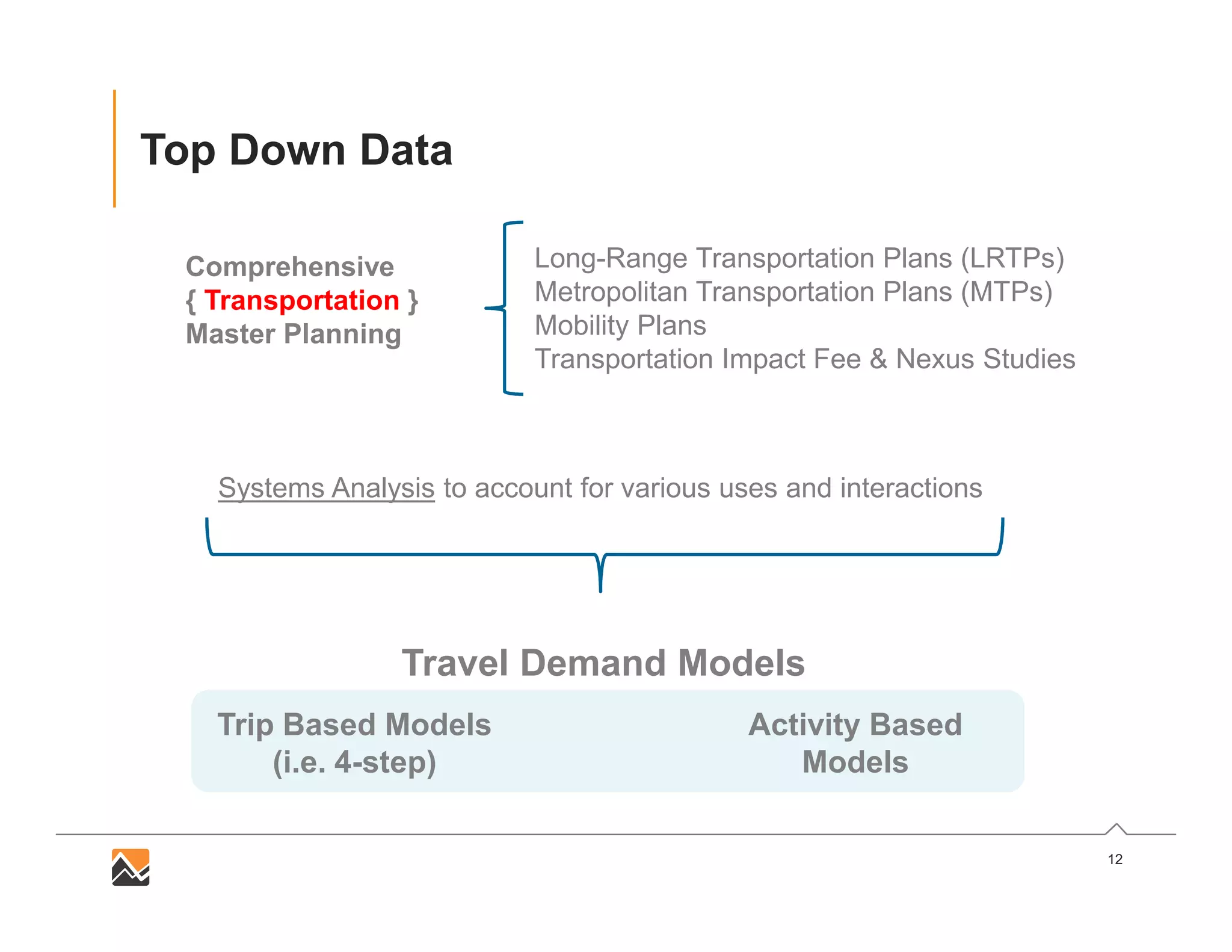
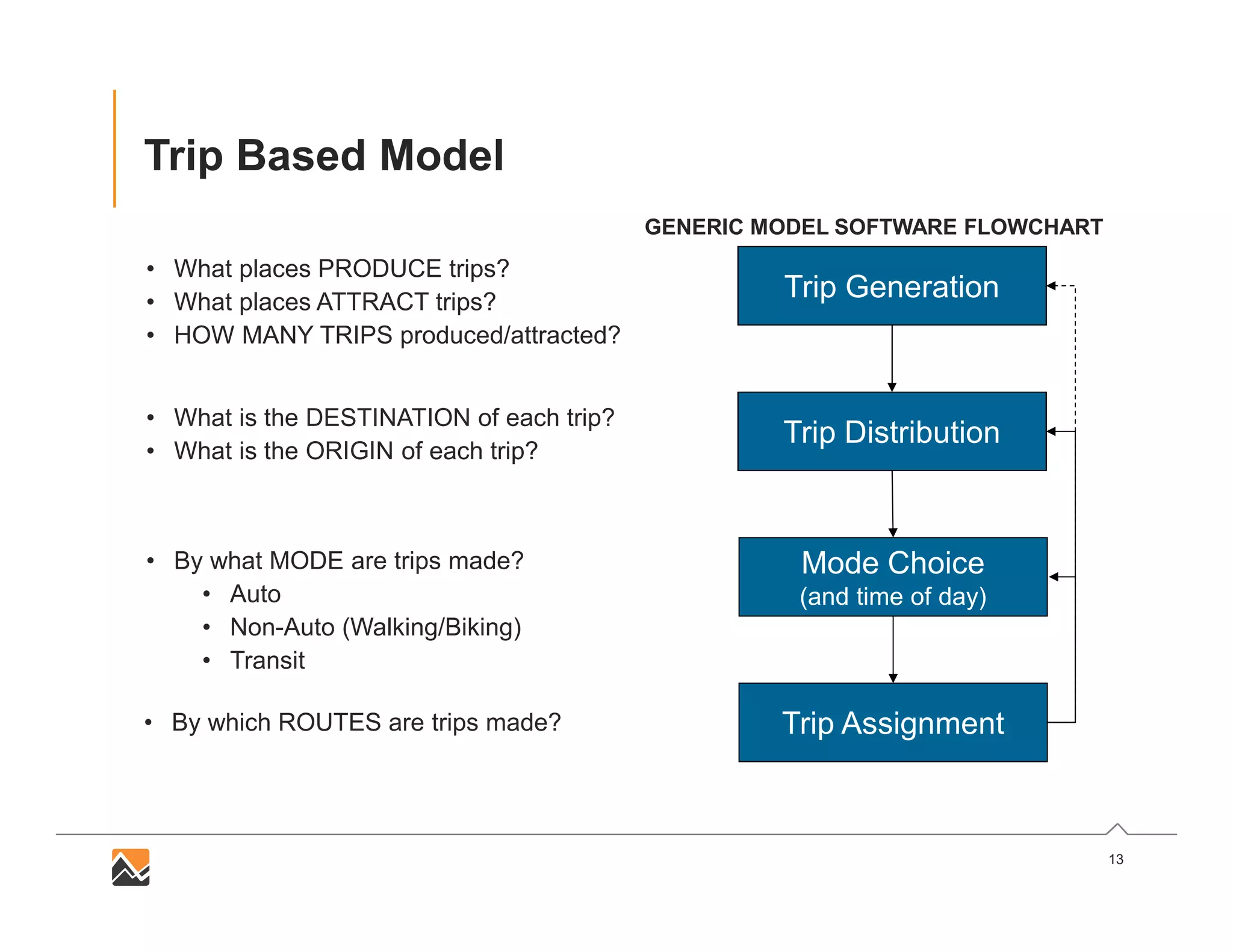
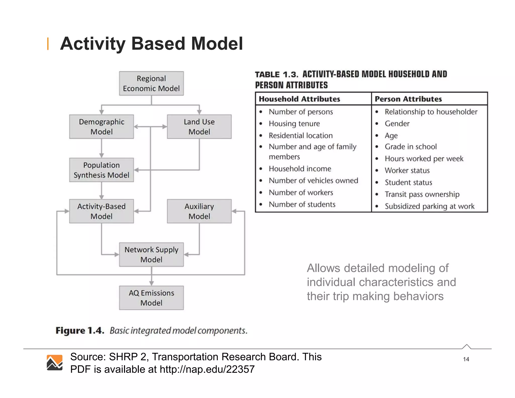
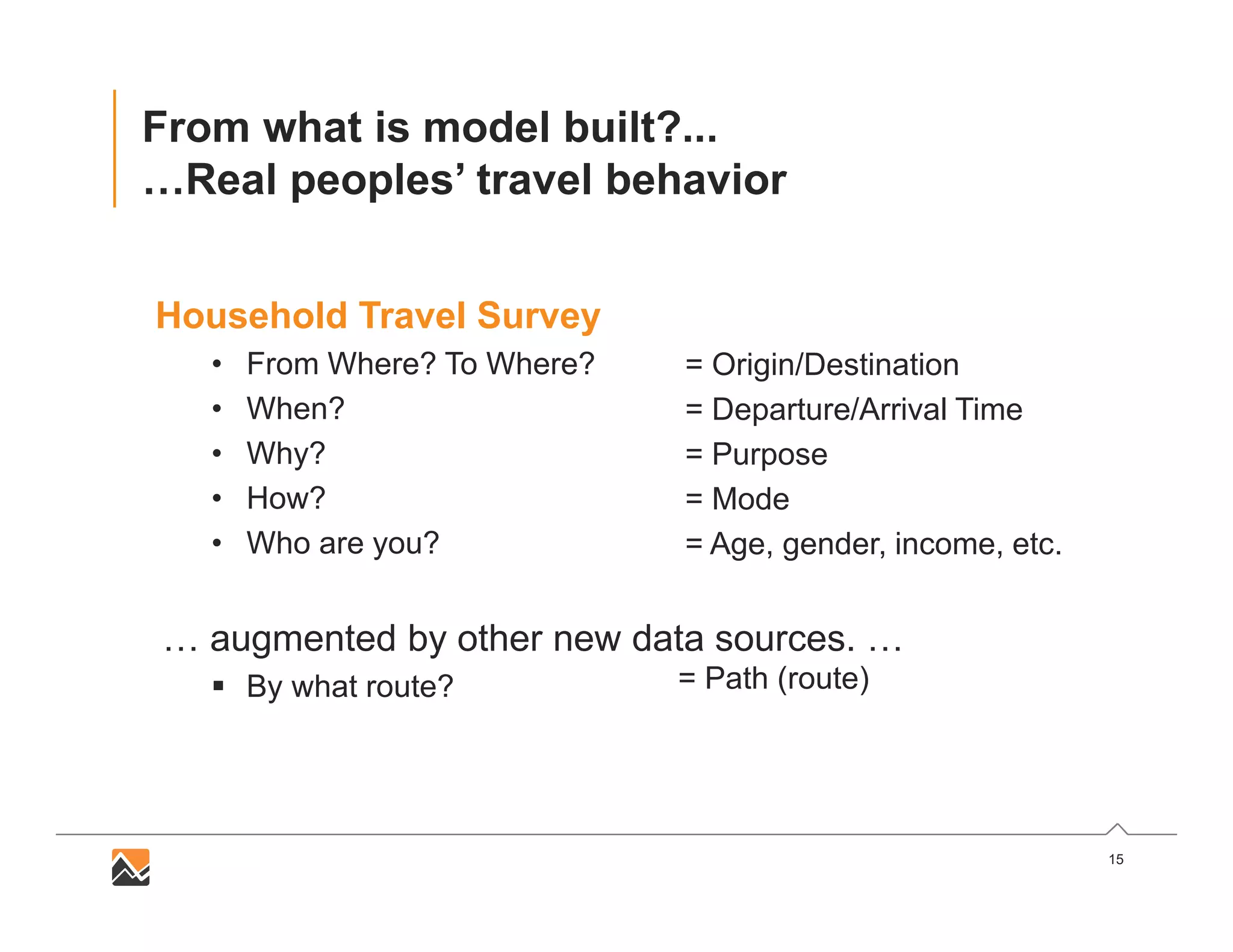
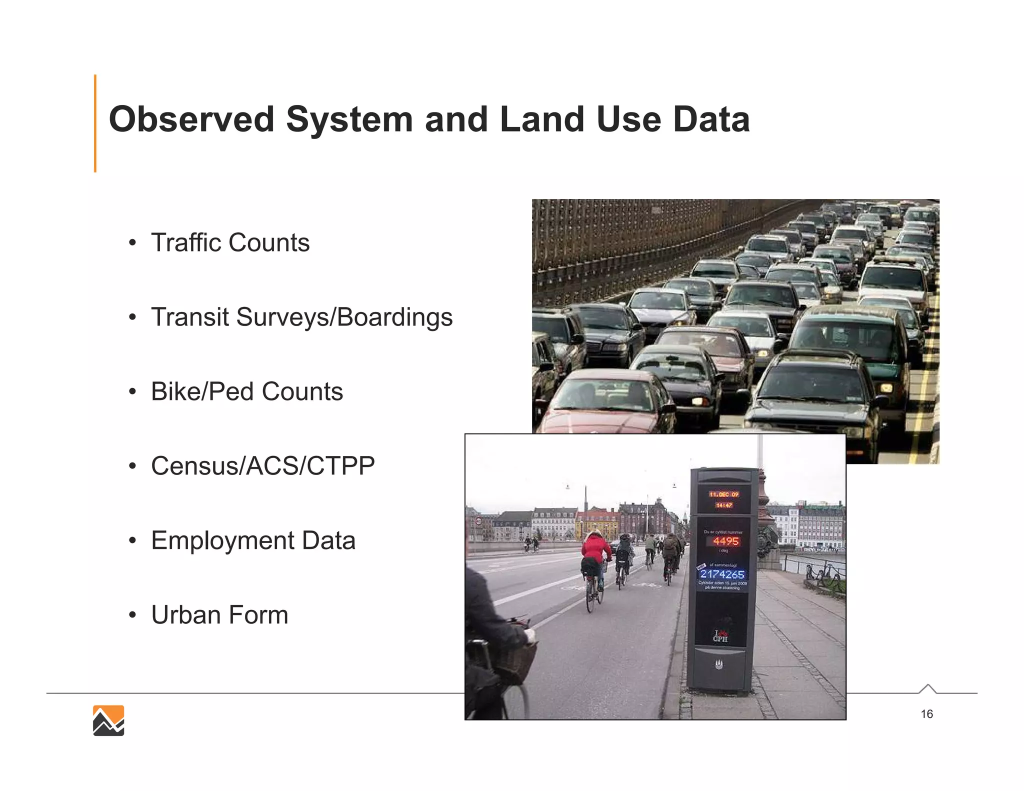
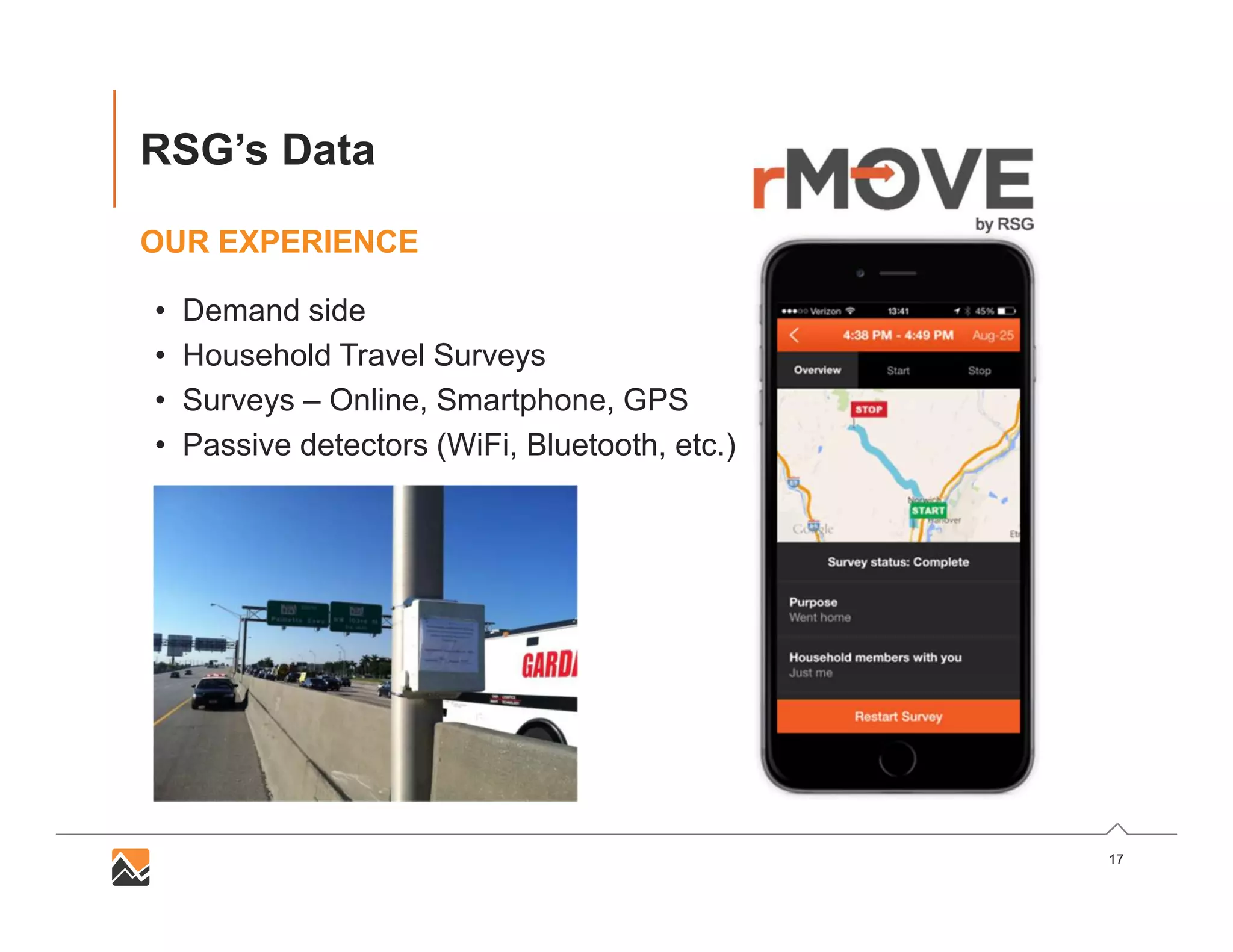
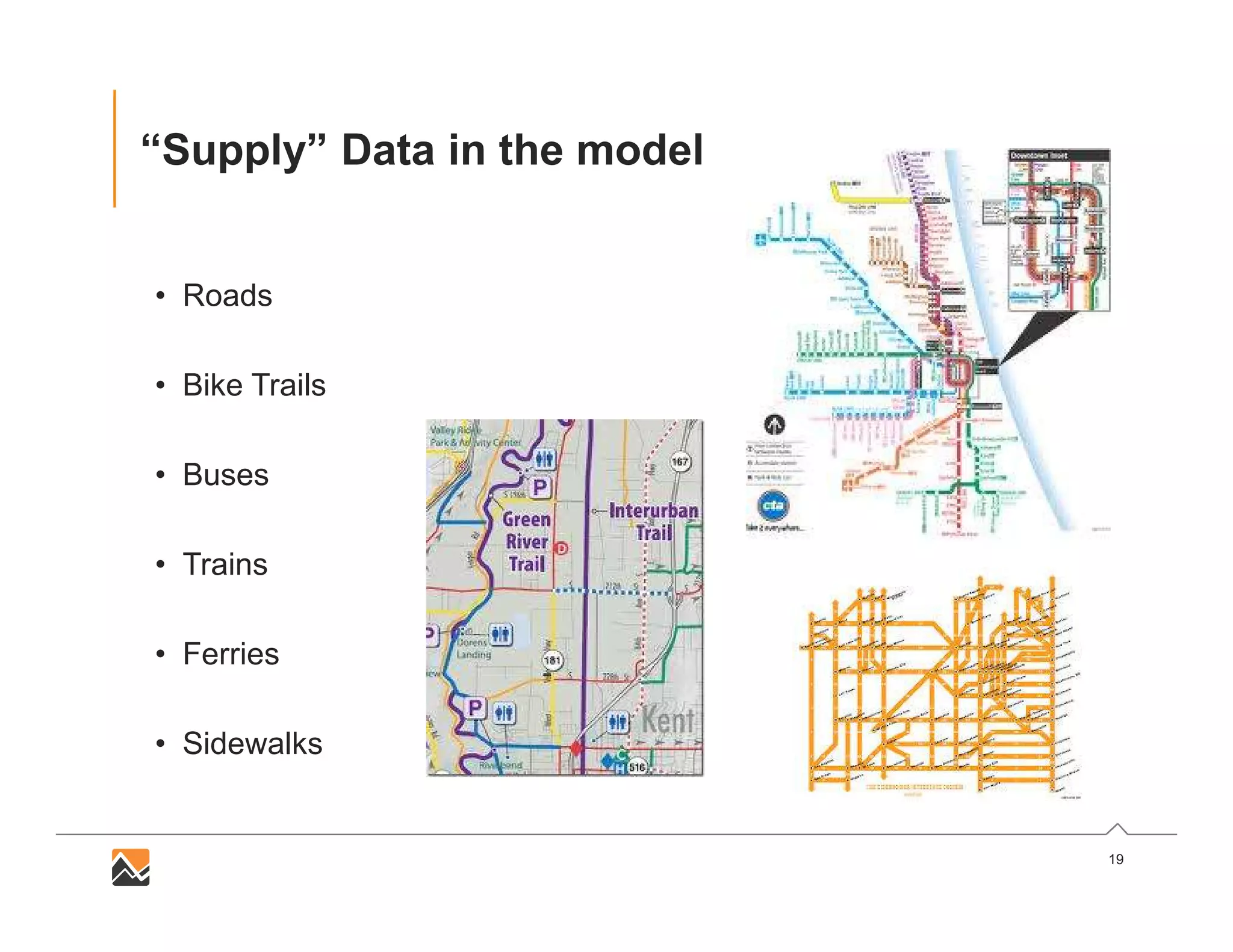
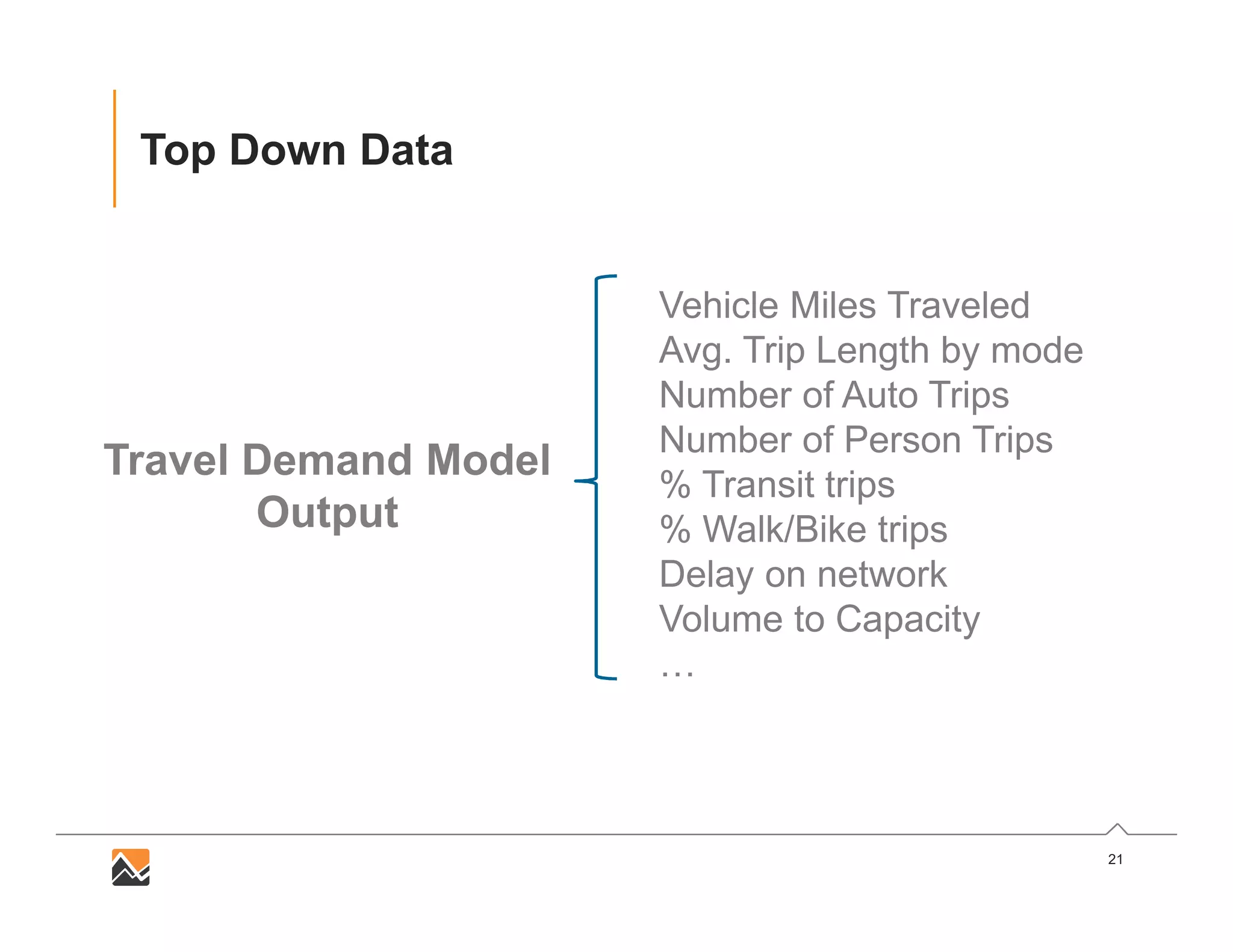
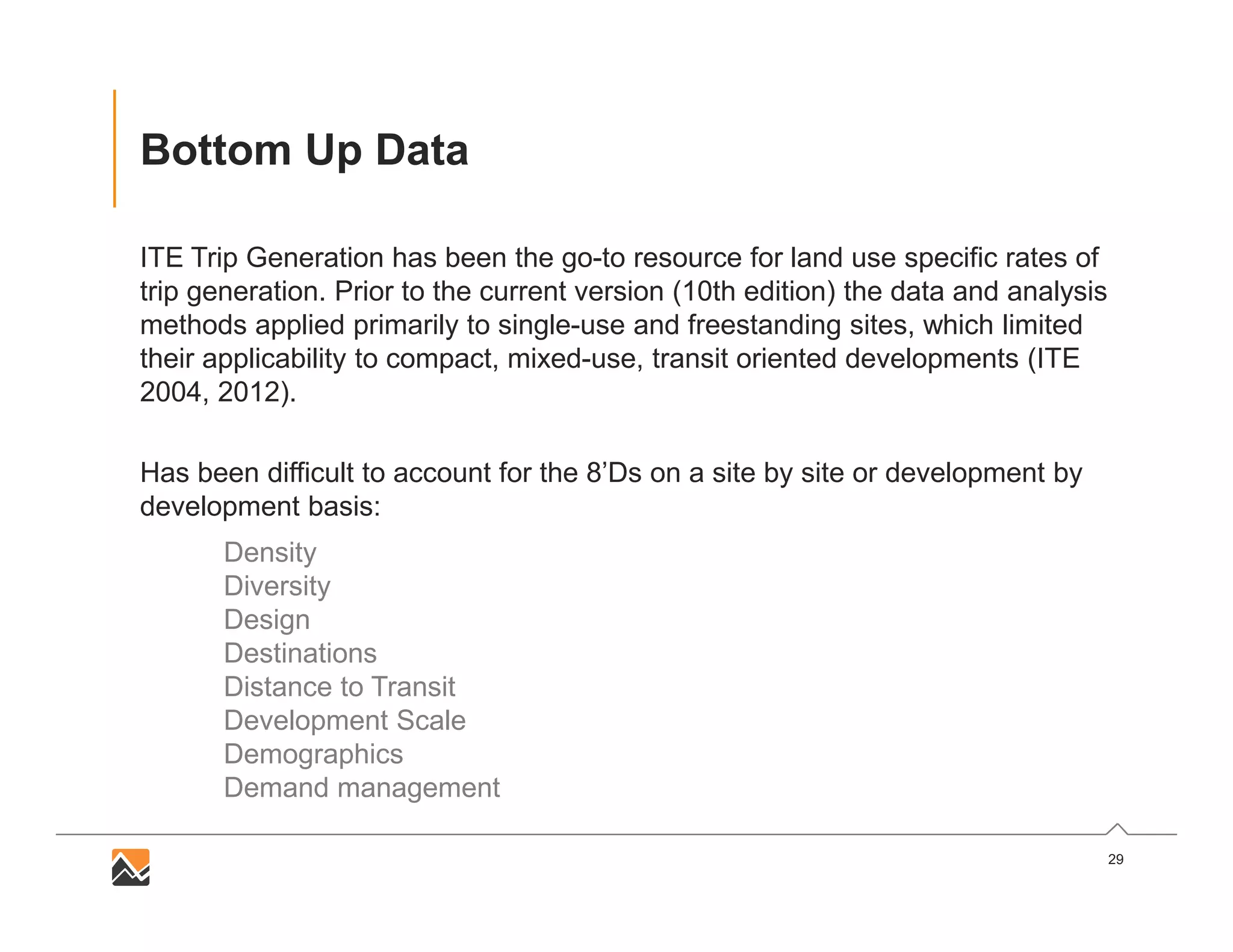
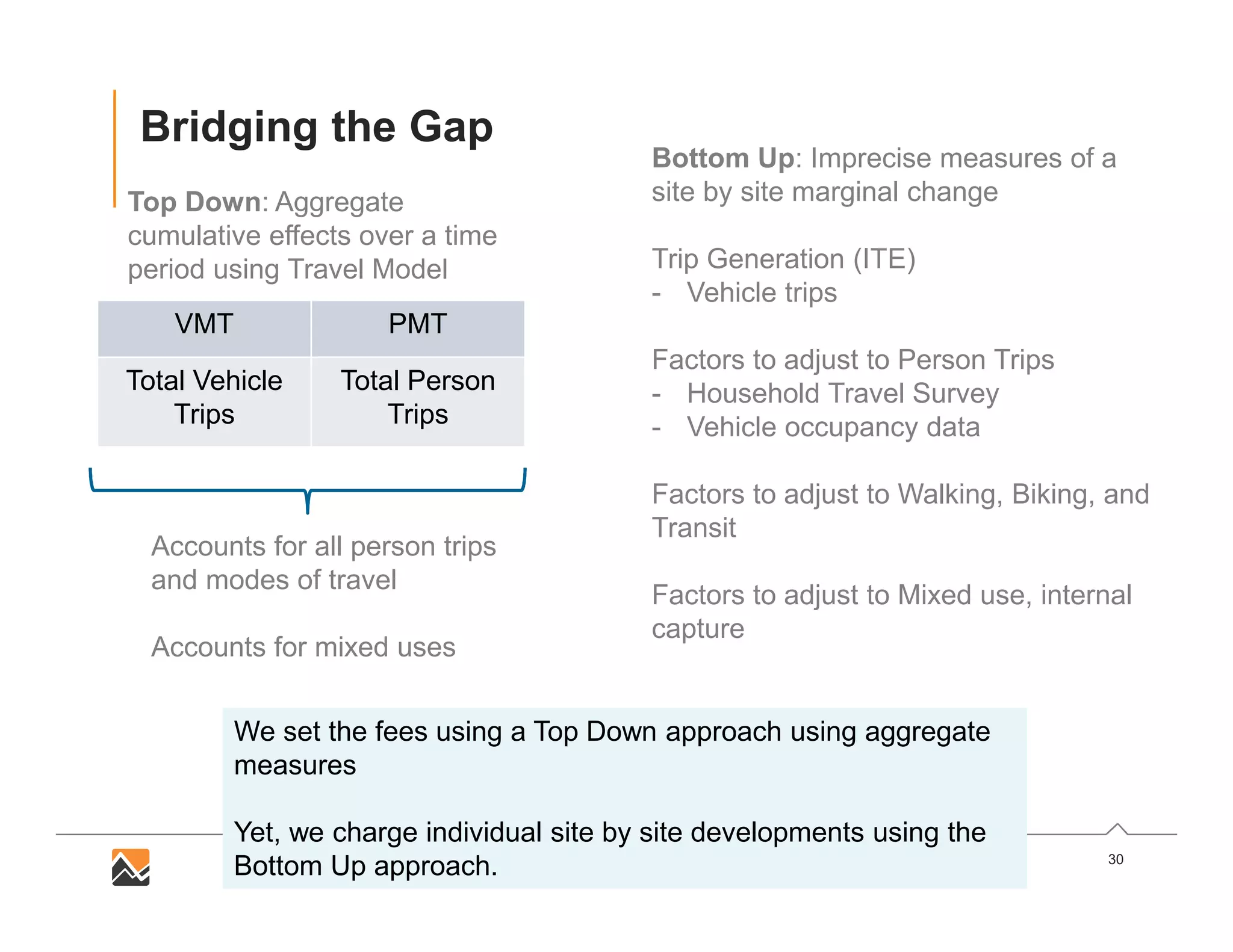
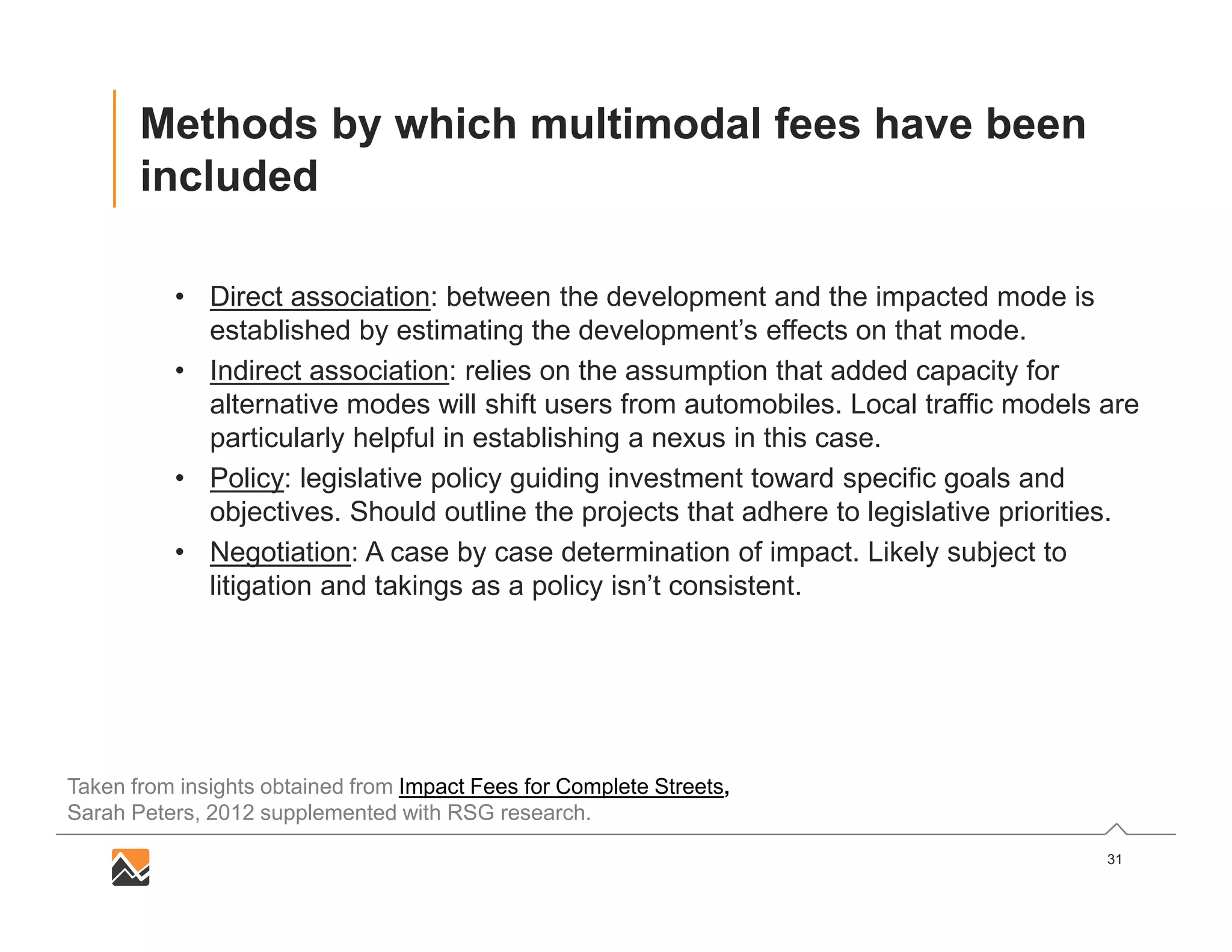
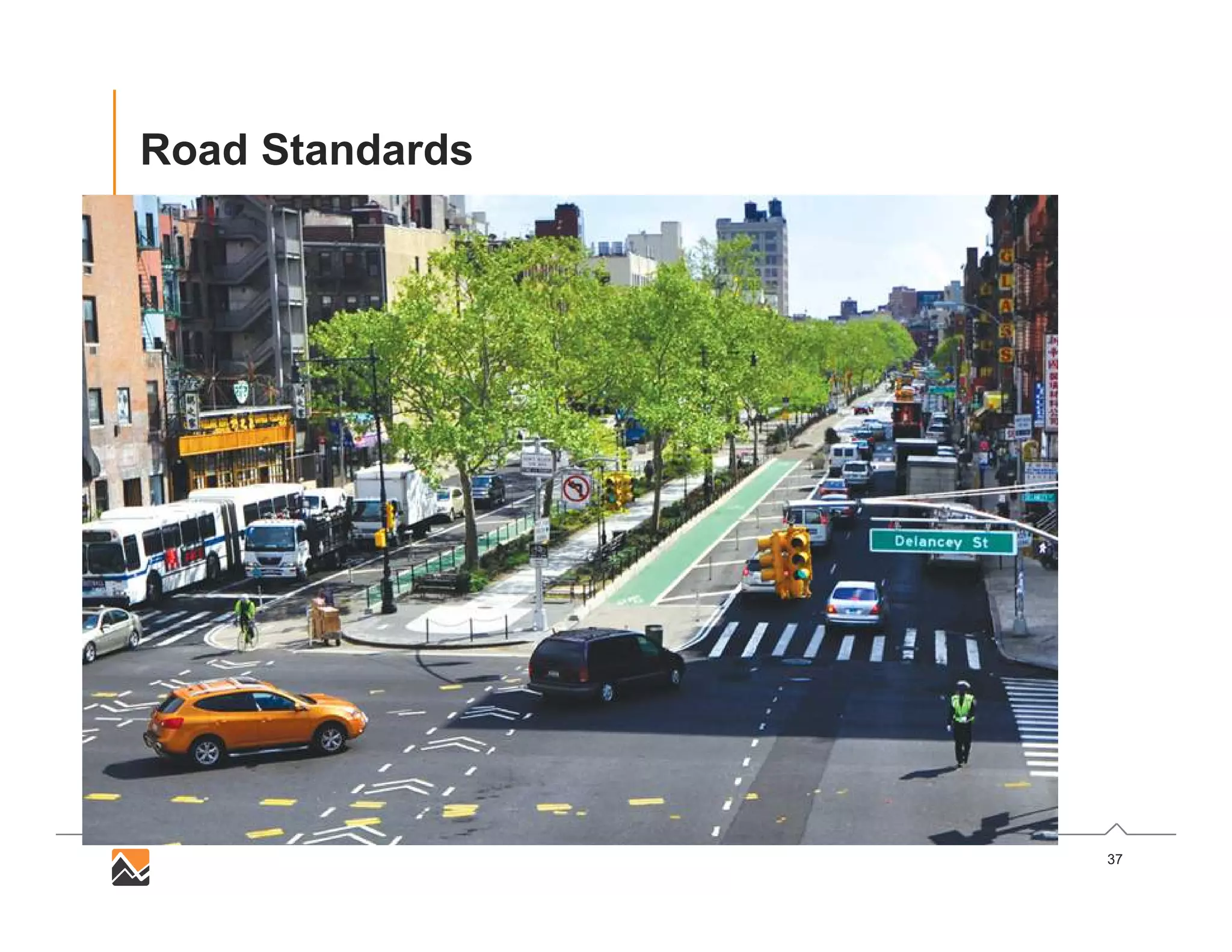
This document discusses transportation impact fees and how to account for multimodal capacity. It notes that comprehensive transportation master planning now incorporates multimodal travel beyond single modes. Land use changes have led to more urban development patterns that support non-auto travel. Transportation impact fees are used to fund necessary mobility infrastructure for new development but traditionally focused on roads; there are now challenges in properly accounting for and assessing multimodal demand and capacity. The document discusses using both top-down data from travel demand models and bottom-up site-specific data to bridge this gap and set multimodal transportation impact fees.

1. Modeling to inform Transportation
Impact Fees – Multimodal
Considerations
GIC 2017 Conference – Sarasota
19 October 2017

2. 2
Comprehensive Master Planning
Covers large area
Long time horizon (10-40 years)
Accounting for:
- Land uses
- Jobs and employment
- Health
- Public safety
- Environmental protection
- Public engagement and input

3. 3
Comprehensive { Transportation } Master Planning
Early comprehensive plans were
single mode
Transition over the last twenty+
years to incorporate and provide
legal footing of multimodal travel.
New tools are coming online and
research is starting to mature
Capacity and trip sheds for non-
auto trips

4. 4
Land Use Changes

5. 5
Land Use Changes
Source: RSG and TransitCenter research in 2013
https://www.planetizen.com/node/86755/what-millennials-want-and-why-it-doesnt-matter

6. 6
Land Use  Multimodal Travel
Impact Fees were relied to fund suburban growth. But the suburbs are maturing.
More urban features being desired in the ‘burbs
As land use has become increasing
more diverse in proximity, mixed use
developments (MXD), transit oriented
development (TOD), and generally
more urban conditions have resulted
in greater emphasis on non-auto
travel.
For both mature cores and suburban
areas

7. 7
The Multimodal future
Many communities are implementing Complete Street policies, which are designed
and operated to make it easy to cross the street, walk to shops, and bike to work
for pedestrians, bicyclists, motorists and transit riders of all ages and abilities.

8. 8
Brief incomplete history of multimodal
Transportation
Roads and vehicular capacity has been a common infrastructure and capital
cost component within impact fees once non-utility (water/sewer) capital
items started to be included.
Many of the roads being funded had costs that included a variety of
elements, sometimes shoulders that could be bike lanes, grass and utility
strips that could include sidewalks. However, the primary measure of service
standard was vehicular capacity.
Increasing demands for multimodal infrastructure – straining the rational
nexus – as we look to the same tools to assess demand and capacity
We know about vehicles - methodology has been around since the
1950’s for vehicle generation, capacity, and levels of service.
Non-Auto LOS only since 2000 Highway Capacity Manual

9. 9
Transportation Impact Fees
A mechanism to facilitate the payment of funds to cover or offset the costs of
necessary mobility capacity that enables the future users to travel on public
infrastructure*.
• How do we arrive at those needs?
• How do we know if we are providing adequate capacity for that growth?
• How do we set the standards of service?
*Several caveats, limitations and rules for them to be applied.

10. 10
No more sweeping
those multimodal
projects under the rug

11. 11
Transportation Impact Fees
How do we reconcile the demand, provision, and
proper accounting of the Multimodal capacity in
our impact fees?
Challenges between Top Down data and Bottom
Up approaches.
Where is our estimate of total demand coming
from? What are the units?
$
ℎ
FeesFeesFeesFees =
VMT?
PMT?
Vehicle Trips?
Person Trips?

12. 12
Top Down Data
Long-Range Transportation Plans (LRTPs)
Metropolitan Transportation Plans (MTPs)
Mobility Plans
Transportation Impact Fee & Nexus Studies
Systems Analysis to account for various uses and interactions
Travel Demand Models
Comprehensive
{ Transportation }
Master Planning
Trip Based Models
(i.e. 4-step)
Activity Based
Models

13. 13
Trip Based Model
• What places PRODUCE trips?
• What places ATTRACT trips?
• HOW MANY TRIPS produced/attracted?
• What is the DESTINATION of each trip?
• What is the ORIGIN of each trip?
• By what MODE are trips made?
• Auto
• Non-Auto (Walking/Biking)
• Transit
• By which ROUTES are trips made?
Trip Distribution
Mode Choice
(and time of day)
Trip Assignment
Trip Generation
GENERIC MODEL SOFTWARE FLOWCHART

14. 14
Activity Based Model
Allows detailed modeling of
individual characteristics and
their trip making behaviors
Source: SHRP 2, Transportation Research Board. This
PDF is available at http://nap.edu/22357

15. 15
Household Travel Survey
• From Where? To Where?
• When?
• Why?
• How?
• Who are you?
… augmented by other new data sources. …
 By what route?
= Origin/Destination
= Departure/Arrival Time
= Purpose
= Mode
= Age, gender, income, etc.
= Path (route)
From what is model built?...
…Real peoples’ travel behavior

16. 16
• Traffic Counts
• Transit Surveys/Boardings
• Bike/Ped Counts
• Census/ACS/CTPP
• Employment Data
• Urban Form
Observed System and Land Use Data

17. 17
RSG’s Data
OUR EXPERIENCE
• Demand side
• Household Travel Surveys
• Surveys – Online, Smartphone, GPS
• Passive detectors (WiFi, Bluetooth, etc.)

18. 18
What about Big and Passive Data Collection?

19. 19
“Supply” Data in the model
• Roads
• Bike Trails
• Buses
• Trains
• Ferries
• Sidewalks

20. 20
“Supply” Data – Multimodal linkage
Travel Models treat non-vehicle trips in a
variety of ways.
• Directly model the non-vehicle trips in the
modeling process
– Trip generation or Activity based
– Assignment to a non-vehicle network
• Indirectly model the non-vehicle trips
– A number of generated trips are not assigned to a
network
• Most models struggle to capture the full
number of trips, especially home based
other and non-homed other (walking dogs,
recreation, etc.)
Generation is done either
on a basis of rough
calibration of factors that
affect non-motorized
demand. These include:
- Density,
- Walkable
- Number of intersections
- Origins and Attractors
proximate
Advanced models are
starting to use
demographic specific
models to forecast demand

21. 21
Top Down Data
Travel Demand Model
Output
Vehicle Miles Traveled
Avg. Trip Length by mode
Number of Auto Trips
Number of Person Trips
% Transit trips
% Walk/Bike trips
Delay on network
Volume to Capacity
…

22. 22

23. 23

24. 24
Some models can incorporate factors of
cycling demand
Bridge path
Bridge bike lane
Bike path
Bike boulevard
Mixed traffic 10k
Mixed traffic 20k
Mixed traffic 30k
Stop/mi
Signal/mi
Turn/mi
Unsig. cross 5k/mi
Unsig. cross 10k/mi
Unsig. cross 20k/mi
Unsig. left 10k/mi
Unsig. left 20k/mi
upslope 2-4%
upslope 4-6%
upslope 6%+
-120 -100 -80 -60 -40 -20 0 20 40 60 80 100
Cyclist willing to travel...
% less % more
If base facilty
isbike lane
Source: Joe Broach, Portland State University

25. 25
User choice - Model Estimation Results
Variable Estimate t-statistics
Alternative-specific constant for bicycle -3.930 -12.67
Person-level attributes
Female -0.695 -12.80
Age 0.088 8.51
Age2/100 -0.109 -9.91
Age missing 1.430 4.71
Some flexibility in work schedule 0.198 3.15
Full flexibility in work schedule 0.249 2.61
Transit pass provided by employer 0.366 3.69
Long-term parking cost at workplace 0.047 3.04
Household-level attributes
Presence of children age 0-4 in the household -0.165 -1.70
Presence of children age 5-15 in the household 0.153 2.42
Income < $15K × household has no car 0.479 2.18
One other household member owns and uses a bicycle regularly 1.860 31.74
Two other household members own and use bicycle regularly 1.880 15.50
Three or more household members own and use bicycle regularly 2.340 9.69
Land-use and bicycling environment-related attributes
Intersection density within half-mile radius of home TAZ 0.004 6.08
Ln(home bike accessibility to indoor recreation (arts & entertainment employment)) 0.111 2.35
Residuals from regressing bike utility on distance between home and workplace 0.025 4.07
Residuals from regressing bike utility on distance between home and school 0.048 3.13
Model Fit Statistics
Number of observations 9,059
Log-likelihood with coefficients = 0 -6,279.22
Final log-likelihood -4,336.91
Adjusted rho-square 0.306
Source: RSG presentation for Portland Oregon Metro. John Gliebe. 18 May 2015.
http://slideplayer.com/slide/7601631/

26. 26
Compare Future Scenarios

27. 27

28. 28

29. 29
Bottom Up Data
ITE Trip Generation has been the go-to resource for land use specific rates of
trip generation. Prior to the current version (10th edition) the data and analysis
methods applied primarily to single-use and freestanding sites, which limited
their applicability to compact, mixed-use, transit oriented developments (ITE
2004, 2012).
Has been difficult to account for the 8’Ds on a site by site or development by
development basis:
Density
Diversity
Design
Destinations
Distance to Transit
Development Scale
Demographics
Demand management

30. 30
Bridging the Gap
Top Down: Aggregate
cumulative effects over a time
period using Travel Model
Bottom Up: Imprecise measures of a
site by site marginal change
Trip Generation (ITE)
- Vehicle trips
Factors to adjust to Person Trips
- Household Travel Survey
- Vehicle occupancy data
Factors to adjust to Walking, Biking, and
Transit
Factors to adjust to Mixed use, internal
capture
Accounts for all person trips
and modes of travel
Accounts for mixed uses
We set the fees using a Top Down approach using aggregate
measures
Yet, we charge individual site by site developments using the
Bottom Up approach.
VMT PMT
Total Vehicle
Trips
Total Person
Trips

31. 31
Methods by which multimodal fees have been
included
• Direct association: between the development and the impacted mode is
established by estimating the development’s effects on that mode.
• Indirect association: relies on the assumption that added capacity for
alternative modes will shift users from automobiles. Local traffic models are
particularly helpful in establishing a nexus in this case.
• Policy: legislative policy guiding investment toward specific goals and
objectives. Should outline the projects that adhere to legislative priorities.
• Negotiation: A case by case determination of impact. Likely subject to
litigation and takings as a policy isn’t consistent.
Taken from insights obtained from Impact Fees for Complete Streets,
Sarah Peters, 2012 supplemented with RSG research.

32. 32
Bridging the Gap
• Realizing this can help communicate the Rational Nexus of multimodal
investments. Often, only on a systemwide basis can the benefits be observed.
• Using a Travel Demand Model and off-model network GIS tools can help
establish the Direct Relationship between development and the impacted mode.
The demands raised by Nollan and Dolan are best met with a quantifiable
measure of supply and demand by all modes.
• In the absence of model data, Indirect Relationships have been frequently used,
suggesting that stating that better pedestrian and bicycle infrastructure attracts
users, provide mobility, and possibly move some auto users to become non-auto
trips.
• A robust Travel Demand Model can assist turn that indirect relationship into a
direct Relationship by attributing specific PMT to non-auto modes or show
reductions in VMT due to other investments.
• Policy-based determinations set by Municipalities could guide the use of Impact
Fees for specific multimodal investment. The clearly defined list of expenditures
and rational for each project articulates and defines the Policy.

33. 33
Cost of Modal Capacity – All Projects
Corridor Projects
Standalone
Bike
Standalone Ped % of Cost of Capacity by Mode and Zone
Mobility
Zone
Vehicle
Capacity
Bike Capacity
Pedestrian
Capacity
Bike Capacity Ped Capacity Road Bike Ped Transit
1 $ 70,411,990 $ 27,812,294 $4,572,466 $15,748,997 $1,383,092 59% 36% 5% 0%
2 $ 78,084,150 $10,141,304 $1,413,356 $2,394,130 $1,481,213 78% 13% 3% 6%
3 $ 129,688,760 $ 83,978,170 $11,877,571 $10,468,537 $1,345,308 54% 40% 6% 1%
4 $ 72,912,144 $ 39,435,755 $7,137,601 $4,625,428 $763,183 58% 35% 6% 0%
5 $ 36,879,382 $14,805,070 $2,036,203 $7,468,097 $2,192,636 58% 35% 7% 0%
6 $ 48,837,445 $15,696,942 $3,683,612 $12,460,038 $1,149,500 60% 34% 6% 0%
7 $ 1,372,931 $ 869,266 $131,803 $6,817,412 $1,551,211 11% 59% 13% 18%
8 $ 50,024,738 $6,259,915 $808,787 $17,365,486 $1,172,383 60% 28% 2% 9%
9 $ 23,506,845 $0 $0 $17,614,662 $4,207,820 47% 35% 8% 10%
Modal Cost
as a
% of Total
Cost
57.5% 22.3% 3.5% 11.4% 2.0% 2.6%

34. 34
Another point of view?
What happens with rational nexus if the design standards
change?
- Water Pipes: Do pipes get more expensive?
- School construction costs?
- Transportation corridors have become multimodal

35. 35
Water Pipes - standards
1950 pipes: $10 per foot
2010 pips: $36 per foot
(2010 dollars)

36. 36
School Construction Costs
The cost for each new building completed has almost doubled.
In 2001, the median new school — elementary, middle and high schools
combined — cost $12,963,000.
In 2013, the median new school cost was $25,671,000.
1. Distribution of schools. The need for new school buildings starts in the elementary
grades and reaches high schools later. Elementary schools declined and instead
constructing middle and high schools.
2. Construction costs overall have increased. The median building completed in 2001
cost about $105 per square foot. The 10 percent of districts that spent the most money
stayed under $200 per square foot.
Among new schools completed in 2013, using the same methodology for calculating costs,
the median elementary school cost more than $200 per square foot and the median high
school almost $250.
3. Sophistication and quality. Greater needs for technologies and amenities.
Source: https://webspm.com/Articles/2014/02/01/School-Buildings-Costs.aspx

37. 37
Road Standards

38. 38
Changing expectations

39. 39
Things are changing…
2017 Release of the ITE Trip Gen Handbook, 3rd Edition
The data collection and analysis approaches presented in this Handbook move toward collection
and application of person trip-level data (from previously vehicle-centric data collection and
consideration).
While the future direction of this Handbook is moving toward more multimodal and detailed person-
level data collection and application, it is well understood that this new approach and methodology
must include some ability to transition from the exclusive use of vehicle-based data to information
that is more inclusive of planning for all modes. ITE trip generation data are intended for uses
associated with site trip generation; that is, trip generation associated with buildings and related
facilities of individual developments. These data are not intended for regional planning activities
beyond facilities adjacent to and near the study site. Corridor scale transportation requirements and
improvements are better determined with the aid of a regional travel demand model, metropolitan
transportation surveys, census data, and related data sources.
Nearly all data presented in the current Trip Generation Manual data volumes have been collected
at low-density, single-use, homogeneous, general urban or suburban developments with little or no
public transit service and little or no convenient pedestrian access. These proxy sites are called
baseline sites in this Handbook because they are the starting points for most vehicle trip generation
estimation recommended in the following chapters.
Trip Generation Handbook , 3rd Edition

40. 40
Things are changing…
Future transportation modes
The traditional measures of LOS will go by the way side.
More often going to be guided by travel times for certain modes, proximity
to modes, safety.
Higher congestion on our roads due to shared vehicles, autonomous
vehicles, - but maybe we tolerate it more because we are doing other
“productive” activities.
Transit, walking, and biking trips have been affected by transportation
network companies and will continue to be affected by CAV growth.
Trip Generation Handbook , 3rd Edition

41. 41
Summary thoughts
Person trips are the fundamental mode. ITE is starting to provide
tools to assess an estimate person trips for specific locations.
Travel Models can be used to assess what degree of demand
multimodal facilities can be expected. Strong direct association
between specific investments and future mobility.
New community expectations in roadway and street designs need
to be incorporated into our basic concept of what constitutes
minimum facilities providing transportation mobility.

42. Contacts
www.rsginc.com
Contacts
www.rsginc.com
Jonathan Slason
Senior Engineer
Jonathan.slason@rsginc.com
802-861-0506