This document is an acknowledgements section from a Master's Thesis on the Anderson model. It thanks several people for their contributions: - The instructor, Professor Martti Salomaa, for introducing the topic, providing guidance and sharing insights. - Dr. Juha Fagerholm for helping develop computational code and advising on programming. - Dr. Robert Joynt for teaching basics of superconductivity. - Colleagues for assistance with LaTeX and other software. - The whole laboratory for creating an inspiring work environment.

1. Acknowledgements
This Master’s Thesis was carried out in the Materials Physics Laboratory
at Helsinki University of Technology. I wish to express my gratitude to
my instructor, professor Martti Salomaa, for introducing me to the fasci-
nating world of Green’s functions, for providing me with a stimulating and
instructive research problem, for sharing his insight and for his quidance. His
experience on this field helped me a great deal to succeed in my work.
The most demanding numerical calculations were performed using the
powerful computer resources of the Center for Scientific Computing (CSC).
I am deeply grateful to Dr. Juha Fagerholm, who helped me to develop the
early versions of the FORTRAN code. His advice helped me to avoid many
programming errors.
My warm thanks also go to Dr. Robert Joynt for teaching me the basics
of superconductivity during his visit to the Materials Physics Laboratory.
Furthermore, I am obliged to Associate Professor Matti Kaivola and to my
colleagues Tapani Makkonen and Julius Koskela for being readily available
whenever I had problems with LATEX or other scientific software. I also
wish to thank Jukka Tuomela for mathematical discussions. Finally, I would
like to present my thanks to the whole personnel of the Materials Physics
Laboratory for creating an inspiring working environment.
Espoo, February 12th, 1997
Ari Alastalo

2. Contents
1 Introduction 1
2 Preliminary Considerations 4
2.1 The Anderson Atom . . . . . . . . . . . . . . . . . . . . . . . 5
3 Anderson Model for a Normal Metal 7
3.1 Description of the Hamiltonian . . . . . . . . . . . . . . . . . 7
3.2 Hartree-Fock (HF) Approximation . . . . . . . . . . . . . . . . 7
3.3 Selfenergy to Second Order in U . . . . . . . . . . . . . . . . . 14
3.3.1 Numerical Results . . . . . . . . . . . . . . . . . . . . 17
4 Anderson Model in a Superconductor 22
4.1 Comments on Superconductivity . . . . . . . . . . . . . . . . . 22
4.2 Impurity Scattering T Matrix . . . . . . . . . . . . . . . . . . 24
4.3 Hartree-Fock Theory . . . . . . . . . . . . . . . . . . . . . . . 25
4.3.1 Numerical Results . . . . . . . . . . . . . . . . . . . . 31
4.4 Second-Order (U2
) Selfenergy Theory . . . . . . . . . . . . . . 40
4.4.1 Identification of the Selfenergy Σσ(ω) . . . . . . . . . . 40
4.4.2 Applying Wick’s Theorem . . . . . . . . . . . . . . . . 41
4.4.3 Formulation in the Time Domain . . . . . . . . . . . . 44
4.4.4 Formulation in the Frequency Domain for the Symmet-
ric Zero-Field Situation . . . . . . . . . . . . . . . . . . 49
4.4.5 Density of States and the Selfconsistency Condition . . 51
5 Numerical Results 55
6 Discussion 60
A Double-time Green’s Functions 62
A.1 Definitions of Correlation and Response Functions . . . . . . . 62
A.2 Anticommutator (Correlation) Functions . . . . . . . . . . . . 64
A.3 Commutator (Response) Functions . . . . . . . . . . . . . . . 65

3. CONTENTS vi
A.4 The Fluctuation-Dissipation Theorem . . . . . . . . . . . . . . 66
A.5 Factorization of Correlations . . . . . . . . . . . . . . . . . . . 66
B Commutators 68
C Calculation of the K Part of the T Matrix Gdσ 70

4. Chapter 1
Introduction
For more than fifty years, the anomalous electric and magnetic properties of
dilute alloys formed by adding magnetic impurities to a nonmagnetic metal
have been recognized. Magnetic impurities are those with a moment caused
by partially filled d- or f-electron shells. A minimum in the resistivity-
temperature curve was found, for example, in the alloys of Cu, Ag, Au, Mg
and Zn with Cr, Mn, Fe, Mo, Re and Os as impurities. This was explained
by Jun Kondo [1] using the s − d exchange model (also called the Kondo
model):
H = Hel − BSz + JS · s, (1.1)
which describes a single impurity atom interacting with the surrounding elec-
tron gas. Kondo showed that the resistance minimum is not due to correla-
tions between localized moments but it rather is a true many-body phenom-
enon and results in adding contributions from each moment independently.
Thus the model for a single impurity atom can explain the Kondo effect.
Here Hel is the Hamiltonian for the conduction electrons, BSz is the Zeeman
energy of the impurity in an external magnetic field B and the latter term
is the contact Hamiltonian. Furthermore, s is the conduction-electron spin
density at the impurity site and J is the exchange coupling constant. Kondo
explained the resistance minimum as due to spin-flip scattering between the
conduction electrons and the localized spin.
In the present work, we consider the Anderson model [2] which is related
to the s − d exchange model via the Schrieffer-Wolff transformation [3, 4].
This transformation on the Anderson model produces quite a few terms, of
which the Kondo model is a subset. Thus the transformation does not pro-
duce exactly the Kondo model, and the two models are not identical. It is
known that the Anderson model has a greater variety of behaviour. It has
the more interesting physics. The Kondo model treats the local spin as a

5. 1 Introduction 2
separate entity. The Anderson model treats the local spin as just another
electron. It can undergo exchange and other processes with the conduction
electrons. This makes the model more realistic, and explains the more inter-
esting behaviour.
The Anderson model, originally suggested to describe a magnetic im-
purity atom in an otherwise nonmagnetic metal, has a broad spectrum of
important applications within theoretical condensed matter physics, ranging
from the above-mentioned Kondo phenomena to valence fluctuations, heavy
fermions (periodic Anderson model), chemisorption and quantum dots [5,6].
In addition to the Hubbard model [7], the single-impurity Anderson model is
one of the most fundamental models to describe correlated electron systems.
The Hartree-Fock (HF) solution, proposed by Anderson in his original
paper [2], only gives the linear terms in U correctly and thus applies only in
the nonmagnetic U → 0 limit. For general U, a plethora of different many-
body techniques have been applied to this model, such as Green’s function
decoupling methods [8–10], renormalization groups [11–13], Bethe Ansatz
approach [14], quantum Monte Carlo simulations [15], the non-crossing ap-
proximation [16] and selfenergy theories [17–20]. In one dimension, the An-
derson model can be solved exactly using the Bethe Ansatz. However, the
one-dimensional results are not a useful quide to collective effects in higher
dimension, since there are neither phase transitions nor long-range order in
one dimension at nonzero temperature.
We utilize the equation-of-motion technique for double-time temperature-
dependent retarded and advanced Green’s functions and perform a self-
energy calculation up to second order in the Coulomb interaction, U, both
for a normal metal and for a BCS superconductor. These Green’s functions
are very convenient for applications in quantum statistics and they can be
analytically continued in the complex plane. The main part of the present
work considers the superconductor for which the second-order treatment has
not yet been discussed in the literature. The text is organized as follows.
Chapter 2 gives the definition of the problem. Also the exactly solvable
but nontrivial atomic limit is shortly discussed.
In Chapter 3 we consider the normal metal. The Hartree-Fock and
second-order calculations are performed in detail. The inadequacy of the
HF approximation is discussed. In particular, the HF approximation fails
in the weak-coupling (small Γ/U) limit to produce the atomic limit. The
second-order treatment is shown to give the atomic limit correctly and, fur-
thermore, the well-known low temperature Abrikosov-Suhl resonance is re-
produced. This resonance is a many-body effect. Also the magnetization of
the impurity atom in zero external field as predicted by the HF treatment is
shown not to survive up to second order in U. The numerical results agree

6. 1 Introduction 3
with those presented in literature.
Chapters 4 and 5 cover the central part of this work. We consider the BCS
superconductor. The Hartree-Fock calculation is presented and the strong-
coupling limit, first published by Shiba [21], is reproduced. Some mistakes
in the published U = 0 results [22] are corrected and an interesting strong-
coupling phenomenon is found, the local order parameter of the impurity
level becomes equal in functional form to the BCS gap, ∆. The HF result
for the behaviour of the localized excited states within the energy gap is
studied in detail for different asymmetries and for finite external fields. A
nonphysical spontaneous symmetry breaking in zero field manifests itself as
in the normal metal case. The second-order perturbation treatment removes
this symmetry breaking. Furthermore, we find for the first time new excited
states within the energy gap when the second-order corrections are taken into
account. It is shown that the Hartree-Fock bound state may be recovered as
an average of two separate bound states. To facilitate performing the second-
order calculation in superconductor with finite work, we chose to concentrate
here on the symmetric zero-field situation. However, doing so is justified since
even this simplest limit has not previously been discussed in the literature
to the best of our knowledge.
The results achieved as well as possibilities to measure them experimen-
tally are discussed in Chapter 6.
A series of appendices summarizes the mathematical formalism employed
in this Master’s Thesis. Appendix A presents the required formalism of
double-time retarded and advanced Green’s functions. If the reader desires
further details on these functions, he or she should consult, for example, Refs.
[23–25] cited in the appendix. Appendix B enlists the central commutators
for the Anderson model. They are utilized throughout this work. Appendix C
shows how one performs one of the integrals essential for the superconducting
case. This integration is presented in detail since it caused some trouble
during the analytical work.

7. Chapter 2
Preliminary Considerations
We consider a single magnetic impurity atom embedded in a nonmagnetic
host metal. The situation is modelled via the Anderson Hamiltonian [2] which
can be split into three parts (for derivation, see also Mahan’s book [26]):
HA = Hel + Hatom + HI (2.1)
where
Hatom =
σ
Eσnσ + Un↑n↓ (2.2)
is the atomic Hamiltonian and
HI =
kσ
Vkc†
kσdσ + V ∗
k d†
σckσ (2.3)
describes the admixture interaction of the localized state with the conduc-
tion electrons. Here Eσ is the energy of a singly occupied impurity state
and U is the intra-atomic Coulomb repulsion. In most cases all the other
Coulomb interactions, the interaction between d electrons and conduction
electrons [27] and between different conduction electrons, are not considered
explicitly. Above, σ is the spin index, k is the wavevector and dσ, d†
σ, ckσ
and c†
kσ are the second-quantized annihilation and creation operators for the
localized state and for the conduction electrons, respectively. They obey
the canonical anticommutation rules (B.1). The number operators n are
nσ = d†
σdσ for the d-level and nkσ = c†
kσckσ for the continuum states. For an
introduction to second quantization, see for example Ref. [28]. In this work,
we consider two different host metals, Hel, a normal one (Chapter 3) and a
BCS superconductor (Chapter 4).
The physical situation, modelled via HA (2.1), is represented in Fig. 2.1.
We take the zero of energy to coincide with the Fermi level εF . Here B is

8. 2 Preliminary Considerations 5
kT
f(e)
E
U
e
Vk
*
Vk
B
eF
1
Figure 2.1: Magnetic impurity level interacting with the nonmagnetic host metal.
the external magnetic field that gives rise to Zeeman splitting of the energy
levels (Eσ = E − σB), Vk is a matrix element for electron hopping between
the localized state and the conduction-electron continuum, f(ε) is the Fermi
distribution function (A.13) and kT is Boltzman’s constant k times temper-
ature T. In the following, we use natural units (k = = 1). In some cases U
can be negative [29] but we discuss only the positive U situation as depicted
in Fig. 2.1.
2.1 The Anderson Atom
If the impurity state does not interact with the host metal (Vk = 0), we may
concentrate on the atomic hamiltonian (2.2):
Hatom =
σ
Eσnσ + Un↑n↓.
This is a nonlinear model that can be linearized and solved exactly with the
Hubbard transformation [30]:
A1σ = n−σdσ (2.4 a)
A2σ = (1 − n−σ)dσ. (2.4 b)

9. 2 Preliminary Considerations 6
The d-electron Green’s function for the Anderson atom is now [31] (see Ap-
pendix A for notation):
dσ ; d†
σ
+
z = A1σ ; A†
1σ
+
z + A2σ ; A†
2σ
+
z
=
1 − n−σ
z − Eσ
+
n−σ
z − Eσ − U
.
(2.5)
The poles at z = Eσ and z = Eσ + U of the propagator (2.5) are the single-
particle eigenenergies of the atomic hamiltonian (2.2). It is an educating
exercise to work out the longitudinal and transversal spin and charge suscep-
tibilities within linear response theory for the Anderson atom:
χ (z) = − Sz ; Sz
−
z (2.6 a)
ξ (z) = − Qz ; Qz
−
z (2.6 b)
χ⊥(z) = − S+
; S− −
z (2.6 c)
ξ⊥(z) = − Q+
; Q− −
z . (2.6 d)
Here
Sz =
1
2
(n↑ − n↓) (2.7 a)
Qz =
1
2
(n↑ + n↓ − 1) (2.7 b)
measure the spin and charge imbalance while
S+
=
1
√
2
d†
↑d↓ S−
= S+ †
(2.7 c)
Q+
=
1
√
2
d†
↑d†
↓ Q−
= Q+ †
(2.7 d)
are the spin-flip and charge-transfer operators for the localized state. Some
results of this calculation were published by us last year [32] and a complete
discussion will come out in the near future.
The Anderson hamiltonian in a normal metal (Chapter 3) can be related
to the Kondo model [1] by a canonical transformation as shown by Schrief-
fer and Wolff [3]. This transformation has also been generalized to a BCS
superconductor [4]. The transformation eliminates the interaction Vk to the
first order. Thus, for small values of the coupling Vk, the Schrieffer-Wolff
transformation can be used to isolate those interactions which dominate the
dynamics of the system. In what follows, we perform a perturbation expan-
sion in U up to second order for all values of Vk. We treat both a normal
metal and a BCS superconductor. The normal-metal result is well known [33]
but a similar treatment beyond the Hartree-Fock approximation for a super-
conductor has not been worked out before.

10. Chapter 3
Anderson Model for a Normal
Metal
3.1 Description of the Hamiltonian
In a normal metal, the host contribution to the model (2.1) is (see, for ex-
ample, Ref. [28]):
Hel = HN =
k,σ
εkσnkσ, (3.1)
where εkσ = εk −σB is the dispersion relation for electrons in the conduction
band, and nkσ = c†
kσckσ is their number operator. Consequently, the entire
Hamiltonian reads:
HN
A =
k,σ
εkσnkσ +
k,σ
Vkc†
kσdσ + V ∗
k d†
σckσ +
+
σ
Eσnσ + Un↑n↓.
(3.2)
The bilinear U = 0 limit (resonant level) like the Vk = 0 case (magnetic
atom) is exactly soluble [34].
3.2 Hartree-Fock (HF) Approximation
In what follows, we discuss the Hartree-Fock solution [2,13] for the Hamil-
tonian (3.2). We consider the single-electron d-state propagator Gdσ(z) =
− dσ ; d†
σ
+
z (see Appendix A) and apply the equation of motion (A.2):
z dσ ; d†
σ
+
z = {dσ, d†
σ} + [dσ, HN
A] ; d†
σ
+
z . (3.3)

11. 3 Anderson Model for a Normal Metal 8
Using (B.1) and (B.4 c c), we obtain:
z dσ ; d†
σ
+
z =
= 1 + Eσ dσ ; d†
σ
+
z +
k
V ∗
k ckσ ; d†
σ
+
z + U n−σdσ ; d†
σ
+
z . (3.4)
Next we introduce the Hartree-Fock (mean-field) approximation:
n−σdσ → n−σ dσ (3.5)
and solve for ckσ ; d†
σ
+
z , again using (A.2):
z ckσ ; d†
σ
+
z = {ckσ, d†
σ} + [ckσ, HN
A] ; d†
σ
+
z
= εkσ ckσ ; d†
σ
+
z + Vk dσ ; d†
σ
+
z
⇒ ckσ ; d†
σ
+
z =
Vk
z − εkσ
dσ ; d†
σ
+
z . (3.6)
Thus we find for the d-electron propagator:
z dσ ; d†
σ
+
z = 1 + Eσ +
k
|Vk|2
z − εkσ
+ U n−σ dσ ; d†
σ
+
z
⇒ Gdσ(z) = −
1
z − Eσ − U n−σ − k |Vk|2 (z − εkσ)−1 . (3.7)
For the frequency-dependent retarded propagator we obtain:
Gdσ(ω) = −
1
ω + i0 − Eσ − U n−σ − k |Vk|2 (ω + i0 − εkσ)−1 . (3.8)
Let us consider the term
K(ω) =
k
|Vk|2
ω + i0 − εkσ
(3.9)
in Eq. (3.8). Usually the symbol F(ω) is used here instead of K(ω). However,
we want to use F later for the anomalous Green’s function in the supercon-
ductor [35]. Using the symbolic identity (A.6), we obtain:
K(ω) = P
k
|Vk|2
ω − εkσ
− iπ
k
|Vk|2
δ(ω − εkσ). (3.10)
Above, the first term on the r.h.s. represents an energy shift that can be
taken into account by redefining the value of E relative to the Fermi level or

12. 3 Anderson Model for a Normal Metal 9
the term can be neglected as small [13]. For a broad band of s-electrons, the
second term can be set equal to −iπN(0) |V |2
, where N(0) is the density
of conduction electron states at the Fermi level. Defining:
Γ = πN(0) |V |2
≥ 0 , (3.11)
we may now write for Gdσ(ω):
Gdσ(ω) = −
1
ω − Eσ − U n−σ + iΓ
(3.12)
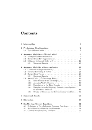
and obtain a Lorentzian density of d-electron states (see Fig. 3.1):
G
′′
dσ(ω) =
Γ
(ω − Eσ − U n−σ )2
+ Γ2
. (3.13)
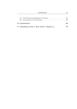
From Eq. (3.12), we see that the excitation energy is shifted due to the
Hartee-Fock selfenergy:
ΣHF
σ = U d†
−σd−σ = U n−σ (3.14)
which can be represented with the familiar tadpole graph shown in Fig.
3.2 [35,36]. Moreover, the interaction with the conduction-electron gas (Γ)
causes the pole of the Green’s function (3.12) to have a nonzero imaginary
part and thus makes the lifetime of the impurity state finite. This means
that the excitations on the impurity state are quasiparticles.
The limitations of the HF approximation can already be observed in Fig.
3.1. Above, discussing the exactly soluble Anderson atom (Γ = 0 -limit),
we found that there exists single-particle excitations at the energies ω = Eσ
and ω = Eσ + U (Eq. (2.5)). Thus, for small but nonzero Γ (0 < Γ < U/2)
we expect two separate lifetime-broadened quasiparticle peaks to remain in
the spectral density, instead of the single peak visible in Fig. 3.1. Therefore,
we conclude that the Hartree-Fock approximation can only be valid for weak
enough interatomic Coulomb-repulsion energies (U < 2Γ).
Combining Eqs. (A.12), (3.13) and (A.13), we obtain an equation for nσ
(in the equal-time limit of Eq. (A.12)):
nσ =
dω
π
1
2
1 − tanh
ω
2T
Γ
(ω − Eσ − U n−σ )2
+ Γ2
. (3.15)
Equation (3.15) is an implicit system of two coupled nonlinear equations of
the form:
nσ = h( n−σ )
n−σ = h( nσ ),

13. 3 Anderson Model for a Normal Metal 10
−10 −1 0 1 10
0
0.5
1
w
G"
Figure 3.1: The Lorentzian density of d-electron states within the Hartree-Fock
approximation for the symmetric Anderson model (E = −U/2) in zero magnetic
field (B = 0) and for small U ( n+ = n− = 1/2). Asymmetry or the external
field only serves to shift the peak in the curve. The halfwidth of the Lorentzian
resonance is 2 Γ. On the horizontal axis, w is the scaled frequency ω/Γ and on the
vertical axis, G
′′
denotes Γ × G
′′
dσ(ω).
U
Gds
d-s d-s
Gds
Figure 3.2: Diagrammatic interpretation of the Hartree-Fock selfenergy, Eq.
(3.14). Solid lines denote the HF propagator and the dotted line represents the
instantaneous Coulomb interaction.

14. 3 Anderson Model for a Normal Metal 11
where h is a nonlinear scalar function of one variable. In the following, we
solve Eqs. (3.15) selfconsistently.
The integral in Eq. (3.15) is complicated by the fact that the function
tanh(z) displays poles at the locations z = −iπ 1
2
+ n , where n ∈ Z. There-
fore, we express the hyperbolic tangent in terms of two digamma functions:
tanh(z) = −
i
π
ψ
1
2
+ i
z
π
− ψ
1
2
− i
z
π
. (3.16)
Here ψ 1
2
+ iz
π
possesses poles in the upper halfplane at the locations z =
iπ 1
2
+ m , where m ∈ N (0 ∈ N), while the poles of ψ 1
2
− iz
π
all reside
in the lower halfplane at the positions z = −iπ 1
2
+ m . Equation (3.16)
follows easily from Eq. (6.3.7) (page 259) in Ref. [37]:
ψ(1 − z) = ψ(z) + π cot(πz) ∀z ∈ C.
Defining
g(ω) = (ω − Eσ − U n−σ )2
+ Γ2
, (3.17)
we are now able to write Eq. (3.15) in the form:
nσ =
Γ
2π
∞
−∞
dω
π
1
g(ω)
I1
+
i
π
∞
−∞
dω
π
ψ 1
2
+ i ω
2πT
g(ω)
I2
−
i
π
∞
−∞
dω
π
ψ 1
2
− i ω
2πT
g(ω)
I3
=
Γ
2π
I1 +
i
π
I2 −
i
π
I3 .
(3.18)
Integrals I1, I2 and I3 can be evaluated using calculus of residues. We close
the integration contour of I2 and I3 in the lower and upper complex half-
planes, respectively, such that the only contribution to the integrals arises
from the poles of 1/g(ω). In I1 we can close the contour, for example, in the
upper halfplane. We obtain straightforwardly:



I1 =
π
Γ
I2 =
π
Γ
ψ
1
2
+
Γ
2πT
+ i
Eσ + U n−σ
2πT
I3 =
π
Γ
ψ
1
2
+
Γ
2πT
− i
Eσ + U n−σ
2πT
.
(3.19)
Thus, combining Eqs. (3.19) and (3.18), we get:
nσ =
1
2
+
i
2π
ψ
1
2
+
Γ
2πT
+ i
Eσ + U n−σ
2πT
+
− ψ
1
2
+
Γ
2πT
− i
Eσ + U n−σ
2πT
.
(3.20)

15. 3 Anderson Model for a Normal Metal 12
Now using the property of the digamma function [37]:
ψ (z∗
) = ψ∗
(z) (3.21)
and defining:
α =
1
2
+
Γ
2πT
, (3.22 a)
ξσ =
Eσ + U n−σ
2πT
, (3.22 b)
we obtain the selfconsistency conditions:
nσ =
1
2
−
1
π
ψi (α + iξσ) . (3.23)
Above, ψi(. . .) denotes the imaginary part of the digamma function.
In the T → 0 limit |α + iξσ| → ∞ and consequently ψ (α + iξσ) →
ln (α + iξσ) [37]. Thus, Eq. (3.23) assumes the form:
nσ =
1
2
−
1
π
arccot
Γ
Eσ + U n−σ
. (3.24)
Setting now the external magnetic field B to zero and defining:
x = −
E
U
, (3.25 a)
y =
U
Γ
, (3.25 b)
we obtain the Hartree-Fock zero-temperature zero-field selfconsistency con-
ditions:
nσ =
1
π
arccot y n−σ − x . (3.26)
Equation (3.26) is easier to utilize at zero temperature than the general
result (3.23) because the digamma function is not included in the standard
mathematical subroutine libraries.
Solutions of Eqs. (3.23) and (3.26) as functions of the level separation
y = U/Γ are illustrated in Fig. 3.3 for different values of the impurity-level
asymmetry x, magnetic field B and temperature T. The magnetization of
the impurity in a vanishing external field for large values of the Coulomb-
repulsion energy U (Figs. 3.3(a-c)) is nonphysical and due to the failure
of the Hartree-Fock approximation which is a linear theory in U. When
second-order corrections (the following section) are taken into account, one

16. 3 Anderson Model for a Normal Metal 13
0 0.5 1 1.5 2
0
0.25
0.5
0.75
1
a
(a)
<n+>
<n+>
<n−>
x=1/2
x=1/16
x=1/4
0 0.5 1 1.5 2
0
0.25
0.5
0.75
1
a
(b)
<n+>
<n−>
t=0
t=0.1t=1
t=10
0 0.5 1 1.5 2
0
0.25
0.5
0.75
1
a
(c)
<n+>
<n−>
t=0t=0.1t=1
t=10
0 0.5 1 1.5 2
0
0.25
0.5
0.75
1
a
(d)
b=0.01
b=0.1
b=1
b=10
b=100
Figure 3.3: Selfconsistent Hartree-Fock solution for the occupation numbers n+
(up) and n− (down) in a normal metal as a function of the inverse Coulomb
interaction a = π/y. The spontaneous symmetry breaking ( n+ = n− ) in zero
field in Figs. (a-c) is an artefact of the HF approximation (see text).
(a): The zero-temperature (T = 0) zero-field (B = 0) solution for asymmetries
x ∈ {1/2 , 1/4 , 1/8 , 1/16}. For increasing asymmetry, the impurity magnetization
occurs for larger values of U.
(b): Spin substate occupations in the symmetric situation (x = 1/2) at finite
temperatures (t = T/Γ ∈ {0 , 1/10 , 1 , 10}) for zero external field (B = 0). For
fixed U, the increase of temperature finally demagnetizes the impurity.
(c): As in (b), but for an asymmetric situation (x = 1/4).
(d): Solution for nonzero magnetic fields (b = B/Γ ∈ {1/100 , 1/10 , 1 , 10 , 100})
at a finite temperature (T = Γ) for the symmetric energy-level configuration (x =
1/2).

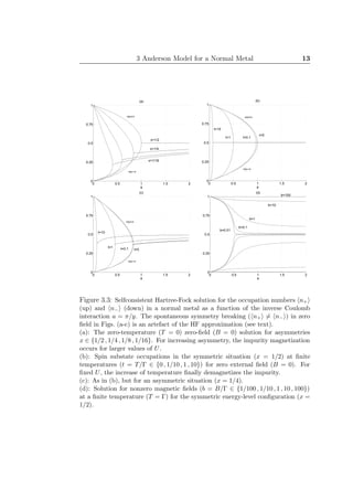
17. 3 Anderson Model for a Normal Metal 14
finds that the spontaneous magnetization in zero field cannot occur. Instead,
one finds equal occupations ( n+ = n− ) for the spin states at all values of
U. Actually, in the magnetic regime, the HF equations (3.23) and (3.26) also
possess the nonmagnetic solution ( n+ = n−
def
= nnm) [2]. However, this
solution is unstable such that if our initial guess for the occupation numbers
differs from nnm, we always end up with nonequal spin state occupations
( n+ = n− ) as shown in Fig. 3.3.
3.3 Selfenergy to Second Order in U
In the following, we extend the theory beyond the HF solution. For U
10πΓ, the selfenergy expansion can be cut after the second-order (U2
) terms.
The higher-order corrections are neglible [33].
Using the Hartree-Fock propagator (3.12) as a basis, we may in general
write a Dyson equation:
dσ ; d†
σ
+
z =
1
z − Eσ − U n−σ + iΓ + Σσ(z)
, (3.27)
where Σσ(z) is the selfenergy. Expanding (3.27) as a geometric series we
obtain:
dσ ; d†
σ
+
z =
1
z − Eσ + iΓ n
U n−σ − Σσ
z − Eσ + iΓ
n
=
=
1
z − Eσ + iΓ
1 +
U n−σ
z − Eσ + iΓ
−
Σσ
z − Eσ + iΓ
+
+O
1
(z − Eσ + iΓ)2 .
(3.28)
Now, let us combine Eqs. (3.4) and (3.6) and avoid the HF approximation
(3.5). One obtains:
(z − Eσ + iΓ) dσ ; d†
σ
+
z = 1 + U n−σdσ ; d†
σ
+
z . (3.29)
Using the equation of motion (A.4) we find the coupling of n−σdσ ; d†
σ
+
z
to a higher-order Green’s function:
(z − Eσ + iΓ) n−σdσ ; d†
σ
+
z = n−σ + U n−σdσ ; n−σd†
σ
+
z . (3.30)
Equations (3.29) and (3.30) now yield:
dσ ; d†
σ
+
z =
1
z − Eσ + iΓ
1 +
U n−σ
z − Eσ + iΓ
+
U2
z − Eσ + iΓ
n−σdσ ; n−σd†
σ
+
z . (3.31)

18. 3 Anderson Model for a Normal Metal 15
Comparing the high-frequency limit of (3.28) with the exact result (3.31)
allows us to identify the second-order selfenergy [38,39]:
Σσ = −U2
n−σdσ ; n−σd†
σ
+
z . (3.32)
Next we obtain the imaginary part of the selfenergy (3.32) using (A.10) and
apply Wick’s theorem [40, 41] to express the emerging six-operator double-
time expectation values in terms of expectation values that contain only
products of two second-quantized fermion operators at different times. These
two-operator expectation values are then obtained with (A.12). Also using
the definition of the delta function:
∞
−∞
dt eiωt
= 2πδ(ω) (3.33)
we find:
Σ
′′
σ(ω) = U2 dω1
π
dω2
π
G
′′
d−σ(ω1) G
′′
dσ(ω2) G
′′
d−σ(ω1 + ω2 − ω)
{[1−f(ω1)][1−f(ω2)] f(ω1+ω2−ω) + f(ω1)f(ω2) [1−f(ω1+ω2−ω)]} . (3.34)
The preceding steps are clarified below in connection with superconductivity.
Formula (3.34) describes the relaxation of d-electron excitations with spin σ
due to localized spin fluctuations with spin −σ. This can be seen more
directly by utilizing Eq. (A.20):
Σ
′′
σ(ω)=U2 dω0
2π
tanh
ω0
2T
+coth
ω−ω0
2T
G
′′
dσ(ω0) χ
′′
−σ(ω−ω0), (3.35)
where χ−σ(ω) = − n−σ ; n−σ
−
ω .
The entire function Σσ is found using the spectral representation (A.5)
and can be cast into a particularly convenient form making use of the equal-
ity:
1
z − s
= −i
∞
0
dλ eiλ(z−s)
, (3.36)
which follows directly from the properties of Laplace transforms. The result
is:
Σσ(z) =
i U2
∞
0
dλ eiλz
[Bσ(λ) B−σ(λ) A−σ(−λ) + Aσ(λ) A−σ(λ) B−σ(−λ)] , (3.37)

19. 3 Anderson Model for a Normal Metal 16
U U
Gds
Gds
s
-s
-s
Figure 3.4: Diagrammatic interpretation of the second-order selfenergy term
(3.37) that describes the relaxation of d-electron excitations with spin σ due to
localized spin fluctuations (susceptibility ”bubble”) with spin −σ.
where we have defined:
Aσ(λ) =
∞
−∞
dω e−iλω
ρσ(ω)f(ω) (3.38 a)
Bσ(λ) =
∞
−∞
dω e−iλω
ρσ(ω) [1 − f(ω)] (3.38 b)
ρσ(ω) =
1
π
G
′′
dσ(ω) = −
1
π
dσ ; d†
σ
+′′
ω (3.38 c)
and f(ω) is the Fermi function (A.13). The selfenergy (3.37) is consistent
with Refs. [36,42] that consider the Hubbard model (HM) [42] and the pe-
riodic Anderson model (PAM) [36]. Consequently, the result (3.37) corre-
sponds to the second-order selfenergy diagram in Fig. 3.4 [36].
The numerical calculation scheme is now as follows. We choose an initial
guess for the occupation numbers nσ and n−σ that define the Hartree-
Fock propagator GHF
dσ (ω) in Eq. (3.12). Using GHF
dσ , we calculate ρσ, Aσ,
Bσ and the selfenergy Σσ with Eqs. (3.38 c a-c) and (3.37), respectively.
Using the selfenergy, we obtain nσ and n−σ to the second order in U with
the help of the Green’s function (3.27). The updated occupations are then
inserted into the HF propagator and the scheme is iterated until convergence.
Alternatively, we could obtain the imaginary part of the selfenergy from
Eq. (3.34) and find the real part numerically from Eq. (A.8) or as in Refs.
[38, 39], we could utilize the factorization (3.35) in order to get Σ
′′
σ. Here
we choose, however, the Fourier-transformation route because it allows us
to utilize the efficient FFT algorithm [43]. Another method for performing
the Fourier integrals effectively utilizes the Poisson-summation formula [44]
that converts the problem into a summation of an infinite alternating series.

20. 3 Anderson Model for a Normal Metal 17
The series summation can then be accelerated, for example, with the help
of the epsilon algorithm [45–47] or using the Levin transformations [48]. We
implemented both the FFT and the Poisson-summation techniques and found
the FFT method faster and sufficiently reliable. However, the numerical error
cannot be reduced much below 10−3
because of the fact that the Lorenzian
Hartree-Fock density-of-states (DOS) (3.13) entering the formulae for Aσ
and Bσ (3.38 a a-b) is a slowly decaying (long-tailed) function for large
frequencies [44]. Below, in Chapter 4, in performing a similar calculation
for a superconductor, we find that the Fourier-transformation method for
obtaining the selfenergy becomes numerically too demanding. It appears to
us, then, that for a superconductor the only way out is to first calculate the
imaginary part of the selfenergy, analogously to Eq. (3.34), and compute the
real part using the Kramers-Kronig relation (A.8).
The imaginary part of the corrected Green’s function Gdσ (or the second-
order density of states) is obtained from Eq. (3.27):
G
′′
dσ(z) =
Γ + Σ
′′
σ
(z − Eσ − U n−σ + Σ′
σ)2
+ (Γ + Σ′′
σ)2 , (3.39)
where Σ
′
σ(ω) and Σ
′′
σ(ω) are the real and imaginary parts of the selfenergy,
respectively. The selfconsistent d-state occupations are found with (A.12):
nσ =
∞
−∞
dω
π
f(ω)G
′′
dσ(ω), (3.40)
where the functional dependence of Gdσ is such that
Gdσ = Gdσ Σσ GHF
dσ ( n−σ ) , GHF
d−σ ( nσ ) .
Thus, we again have a pair of coupled nonlinear equations to solve (one
equation for each spin state). Selfconsistency is achieved when the occupation
numbers entering the Hartree-Fock propagator are the same as those obtained
using Eqs. (3.40) and (3.39).
The selfconsistent solution of equations (3.40) was obtained using the
Newton-Raphson method [49] and utilizing the FFT and Simpson rules [49]
for the integrations.
3.3.1 Numerical Results
We have computed the d-level occupations and densities of states for arbi-
trary values of the asymmetry (x = −E/U), Coulomb-repulsion energy (U),
temperature (T) and magnetic field (B). In what follows, we exemplify our

21. 3 Anderson Model for a Normal Metal 18
results for just one representative value of U, namely U = 3πΓ. This value
is well beyond the applicability of the Hartree-Fock theory and within the
range were the higher-order corrections (U4
, . . .) may be neglected [33].
Figure 3.5 shows the d-electron DOS at various temperatures in the sym-
metric zero-field situation. In the high-temperature (and small Γ) limit, we
observe the lifetime-broadened quasiparticle peaks at the approximate en-
ergies ±U/2 (see the discussion in the previous section in connection with
Fig. 3.1 and Eq. (2.5)). When temperature is lowered, a sharp many-body
Abrikosov-Suhl resonance that approaches the unitary limit is rapidly formed
at the Fermi level. The triple-peaked structure of the T = 0 limit, repro-
duced here, was first obtained by Yamada [33] using Pfaffian determinants.
At high temperatures (Fig. 3.5c) Σ
′′
σ(ω) has a large value at zero frequency,
corresponding to a large relaxation. In the low-temperature limit (repre-
sented by T = 0.01Γ in Fig. 3.5d), low-frequency relaxation is inhibited
(Σ
′′
σ(ω = 0) = 0), thus producing the central resonance.
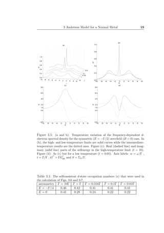
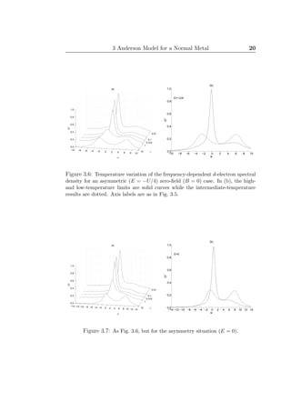
In Figs. 3.6 and 3.7, two asymmetric zero-field situations are considered.
With increasing asymmetry, one sees that the central resonance is broadened
and is no longer pinned to the Fermi level. Simultaneously, the two broad res-
onances are smeared out in the low-temperature limit and finally they disap-
pear completely leaving us with the Hartree-Fock result: a single Lorentzian
peak. The correlation effects are thus found to be most pronounced in the
symmetric situation and strongly reduced for increasing asymmetry. If one
were to interpret the central peak with a d-electron quasiparticle in the sense
of Fermi-liquid theory [50], then one recognizes that such a shortening of
a quasiparticle’s lifetime as it is removed from the Fermi level is a generic
feature.
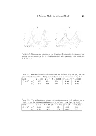
The finite-field case [51] is considered in Fig. 3.8 for the symmetric sit-
uation and for a relatively strong magnetic field. One observes the Zeeman
splitting in the density of states and a transition to the Hartree-Fock result
as temperature is decreased. In the low-temperature limit, the correlation
effects do not show up in the density of states for strong enough fields as in
Fig. 3.8.
Table 3.1 displays the selfconsistently determined d-state occupations for
the situations of Figs. 3.6 and 3.7. In Fig. 3.5, we find n↑ = n↓ =
1/2. The results are consistent with the limiting high-temperature value
n @ > T → ∞ >> 1/2. Table 3.2 enlists the occupation numbers used
in the calculation of Fig. 3.8a (symmetric finite-field case). One observes
a fast transition (see Table 3.3 and Fig. 3.8b) from n↑ ≈ n↓ ≈ 1/2 to
n↑ ≈ 1 n↓ ≈ 0 as thermal energy is lowered below the magnetic-field
energy.

22. 3 Anderson Model for a Normal Metal 19
−10 −8 −6 −4 −2 0 2 4 6 8 10
10
1
0.316
0.1
0.01
0.0
0.2
0.4
0.6
0.8
1.0
w
G"
t
(a)
−10 −8 −6 −4 −2 0 2 4 6 8 10
0.0
0.2
0.4
0.6
0.8
1.0
w
G"
(b)
−10 −8 −6 −4 −2 0 2 4 6 8 10
−4.0
0.0
1.0
2.0
4.0
6.0
8.0
w
S
(c)
−10 −8 −6 −4 −2 0 2 4 6 8 10
−4.0
0.0
1.0
2.0
4.0
6.0
8.0
w
S
(d)
Figure 3.5: (a and b): Temperature variation of the frequency-dependent d-
electron spectral density for the symmetric (E = −U/2) zero-field (B = 0) case. In
(b), the high- and low-temperature limits are solid curves while the intermediate-
temperature results are the dotted ones. Figure (c): Real (dashed line) and imag-
inary (solid line) parts of the selfenergy in the high-temperature limit (t = 10).
Figure (d): As (c) but for a low temperature (t = 0.01). Axis labels: w = ω/Γ ,
t = T/Γ , G
′′
= ΓG
′′
dσ and S = Σσ/Γ.
Table 3.1: The selfconsistent d-state occupation numbers n that were used in
the calculation of Figs. 3.6 and 3.7.
asymmetry T = 10Γ T = Γ T = 0.316Γ T = 0.1Γ T = 0.01Γ
E = −U/4 0.46 0.42 0.41 0.41 0.41
E = 0 0.41 0.28 0.24 0.22 0.22

23. 3 Anderson Model for a Normal Metal 20
−10 −8 −6 −4 −2 0 2 4 6 8 10
10
1
0.316
0.1
0.01
0.0
0.2
0.4
0.6
0.8
1.0
w
G"
t
(a)
−10 −8 −6 −4 −2 0 2 4 6 8 10
0.0
0.2
0.4
0.6
0.8
1.0
w
G"
(b)
E=−U/4
Figure 3.6: Temperature variation of the frequency-dependent d-electron spectral
density for an asymmetric (E = −U/4) zero-field (B = 0) case. In (b), the high-
and low-temperature limits are solid curves while the intermediate-temperature
results are dotted. Axis labels are as in Fig. 3.5.
−14 −12 −10 −8 −6 −4 −2 0 2 4 6 8 10 12 14
10
1
0.316
0.1
0.01
0.0
0.2
0.4
0.6
0.8
1.0
w
G"
t
(a)
−14 −12 −10 −8 −6 −4 −2 0 2 4 6 8 10 12 14
0.0
0.2
0.4
0.6
0.8
1.0
w
G"
(b)
E=0
Figure 3.7: As Fig. 3.6, but for the asymmetry situation (E = 0).

24. 3 Anderson Model for a Normal Metal 21
−10 −8 −6 −4 −2 0 2 4 6 8 10
10
1
0.316
0.1
0.01
0.0
0.2
0.4
0.6
0.8
1.0
w
G"
t
(a)
−10 −8 −6 −4 −2 0 2 4 6 8 10
5
10/9
0.0
0.2
0.4
0.6
0.8
1.0
w
G"
t
(b)
Figure 3.8: Temperature variation of the frequency-dependent d-electron spectral
density for the symmetric (E = −U/2) finite-field (B = 4Γ) case. Axis labels are
as in Fig. 3.5.
Table 3.2: The selfconsistent d-state occupation numbers n↑ and n↓ for the
symmetric situation (E = −U/2) in finite fields used in calculation of Fig. 3.8a.
field T = 10Γ T = Γ T = 0.316Γ T = 0.1Γ T = 0.01Γ
B = 4Γ n↑ 0.56 0.94 0.95 0.95 0.95
n↓ 0.44 0.06 0.05 0.05 0.05
Table 3.3: The selfconsistent d-state occupation numbers n↑ and n↓ as in
Table 3.2, but for temperatures between T = 10Γ and T = Γ (see Fig. 3.8b).
field T = 5Γ T = 10Γ/3 T = 2.5Γ T = 2Γ T = 10Γ/6
B = 4Γ n↑ 0.62 0.68 0.74 0.83 0.88
n↓ 0.38 0.32 0.26 0.17 0.12

25. Chapter 4
Anderson Model in a
Superconductor
4.1 Comments on Superconductivity
Superconductivity was first discovered in the laboratory of Heike Kammerlingh-
Onnes in Leiden in 1911. A sample of Hg was found to have zero resistance -
and thus zero dc power dissipation - below a critical temperature, 4.2K. Since
then, one of the principal goals in the field of superconductivity has been to
attempt finding materials that possess as high a critical temperature Tc as
possible. Modern high-Tc materials are superconducting above 77K, which is
the boiling point of liquid nitrogen. For example, HgBa2Ca2Cu3O8, discov-
ered in 1993, has Tc = 133K. For high-Tc materials, the microscopic theory
and a full understanding of the reasons for superconductivity is still missing.
In 1957, a microscopic theory for the conventional low-Tc superconduc-
tors, the so-called BCS theory, was developed by Bardeen, Cooper and Schri-
effer [52]. The key point was to notice that the normal-metal Fermi sea of
electrons is unstable against an attractive interaction Akk′ between the elec-
trons, no matter how weak Akk′ . This interaction leads to the pairing of
electrons (Cooper pairs) and to the formation of a new macroscopic ground
state. It is understood that the attractive interaction Akk′ in BCS supercon-
ductors is the result of electrons interacting with phonons. One may visualize
this process as an electron disturbing the background ionic lattice, thus caus-
ing an accumulation of positive charge density along the path of the electron.
Another electron is then attracted to this net positive charge.
Above the BCS ground state, the excitation energies for the elementary
excitations are given by:
Ek = ± ξ2
k + ∆2(T), (4.1)

26. 4 Anderson Model in a Superconductor 23
where
ξk = εk − µ. (4.2)
Here εk is the normal-state dispersion relation for the conduction electrons,
µ is the chemical potential and ∆(T) is the temperature-dependent energy
gap. Below Tc, the gap is finite ∆(T < Tc) > 0 and it takes at least an energy
2∆ to break a Cooper pair and excite two electrons into the continuum. At
low temperatures, the only resistance mechanism is elastic scattering from
impurities. If there is a gap for all single-electron excitations, then there are
no final states for an electron at the Fermi surface to scatter into. Therefore,
zero dc resistance results. There is no gap, however for a collective excita-
tion of the following kind: change every electron orbital k to k + q. This
excited state carries a current in the direction of q (if the system has cubic
symmetry). An insulator, in contrast, would also have a gap for this kind of
collective excitation. The gap in an insulator is created by the lattice poten-
tial and therefore comes into play for any electronic motion with respect to
that preferred frame. The superconducting gap is created by inter-electron
interactions. It is manifest if one electron changes its motion with respect to
the center-of-mass motion of the electron system. It does not appear if all
the electrons move together.
Pairing is strongest for electrons that have opposite wavevectors. There-
fore, the so-called reduced Hamiltonian [53]
H =
k,σ
εkσnkσ +
k,l
Vklc†
k↑c†
−k↓c−l↓cl↑ (4.3)
that describes the scattering of Cooper pairs is chosen. A variable that turns
out to be the energy gap is introduced:
∆k = −
l
Vkl c−l↓cl↑ . (4.4)
Furthermore, one usually chooses a constant scattering matrix element Vkl =
−V , such that the energy gap does not depend on the wavevector ∆k = ∆
(s-wave pairing). By introducing the approximate Gorkov factorization [54]:
c†
k↑c†
−k↓c−l↓cl↑ → c†
k↑c†
−k↓ c−l↓cl↑ + c†
k↑c†
−k↓ c−l↓cl↑ , (4.5)
one arrives at the host Hamiltonian for a BCS superconductor:
Hel = HBCS =
k,σ
εkσnkσ −
k
∆c†
k↑c†
−k↓ + ∆∗
c−k↓ck↑ . (4.6)

27. 4 Anderson Model in a Superconductor 24
Consequently, the entire Anderson Hamiltonian (2.1) in a superconductor is:
HBCS
A =
k,σ
εkσnkσ −
k
∆c†
k↑c†
−k↓ + ∆∗
c−k↓ck↑ +
+
σ
Eσnσ + Un↑n↓ +
k,σ
Vkc†
kσdσ + V ∗
k d†
σckσ .
(4.7)
The commutators for the Hamiltonian (4.7) are tabulated in Appendix B. In
what follows, we proceed along the same lines as in the normal-metal case.
However, for the superconductor the calculations are much more involved.
4.2 Impurity Scattering T Matrix
For an introduction to scattering theory, see, for example, Refs. [28,55].
Let us first consider a clean bulk superconductor (H = HBCS). Using
the equation of motion (A.2) and the commutators (B.5 a) (dropping the
impurity terms) one observes that the conduction-electron propagator G0
kk′σ
acquires a 2×2 matrix form (a Nambu matrix in the particle-hole space [56]):
G0
kk′σ(z) =
ckσ ; c†
k′σ
+
z ckσ ; c−k′−σ
+
z
c†
−k−σ ; c†
k′σ
+
z c†
−k−σ ; c−k′−σ
+
z
(4.8)
(note the unusual sign convention chosen here). Consequently, one finds:
z − εkσ 2σ∆
2σ∆∗
z + εk−σ
G0
kk′σ(z) = δkk′ ˆ1.
Thus,
G0
kk′σ(z) = G0
kσ(z) =
z − εkσ 2σ∆
2σ∆∗
z + εk−σ
−1
. (4.9)
Above δkk′ denotes the Kronecker delta, ˆ1 is the 2 × 2 unit matrix and the
superscript 0 refers to the pure BCS state in the absence of the impurity. In
deriving Eq. (4.9), we used ε−k−σ = εk−σ for the conduction-electron disper-
sion relation εkσ. The matrix propagator (4.8) may be written in shorthand
notation by considering the Nambu pseudospinor operator [22,56]:
ψkσ =
ckσ
c†
−k−σ
which results in:
Gkk′σ(z) = ψkσ ; ψ†
k′σ
+
z .

28. 4 Anderson Model in a Superconductor 25
Above, ψ†
k′σ = c†
k′σ c−k′−σ .
Taking now the full Hamiltonian HBCS
A into consideration, one finds that
the conduction-electron Green’s function Gkk′σ, which again is a 2×2 matrix:
Gkk′σ(z) =
ckσ ; c†
k′σ
+
z ckσ ; c−k′−σ
+
z
c†
−k−σ ; c†
k′σ
+
z c†
−k−σ ; c−k′−σ
+
z
, (4.10)
is coupled to the d-electron propagator:
Gdσ(z) = −
dσ ; d†
σ
+
z dσ ; d−σ
+
z
d†
−σ ; d†
σ
+
z d†
−σ ; d−σ
+
z
(4.11)
via:
Gkk′σ = δkk′ G0
kσ − G0
kσ
ˆVkGdσ
ˆV ∗
k′ G0
k′σ . (4.12)
Here we have defined:
ˆVk =
Vk 0
0 −V ∗
k
. (4.13)
The first term in Eq. (4.12) describes the free propagation of conduction
electrons, whereas the second term contains the scattering, determined by
the impurity atom’s T matrix abbreviated with Gdσ. In what follows, we
calculate the T matrix both within the-Hartree Fock approximation and to
the second order in U utilizing a selfenergy expansion, thus generalizing the
treatment of the normal-metal case.
In obtaining Eq. (4.12), we have assumed that the impurity atom alters
neither the BCS gap ∆ nor the energy band εkσ. Also, a symmetric interac-
tion in the momentum space (Vk = V−k) has been chosen.
4.3 Hartree-Fock Theory
We use the equation of motion (A.4) for the components of the d-electron
Green’s function Gdσ and introduce the mean field approximation:
d†
−σd−σd†
σ → n−σ d†
σ − d†
−σd†
σ d−σ
d†
σdσd−σ → nσ d−σ + dσd−σ d†
σ
. (4.14)
Note that in the normal metal (∆ = 0 limit), the anomalous expectation
values dσd−σ and d†
−σd†
σ = dσd−σ
∗
vanish, leaving us with the HF ap-
proximation for the normal metal (3.5). Substituting Eq. (4.14) into the
equations of motion allows one to write for the impurity scattering T matrix:
Gdσ(z) = [Kσ(z) − Pσ(z)]−1
. (4.15)

29. 4 Anderson Model in a Superconductor 26
Above, we define
Pσ(z) =
z − Eσ − U n−σ U dσd−σ
U d†
−σd†
σ z + E−σ + U nσ
(4.16)
and
Kσ(z) =
k
ˆV ∗
k G0
kσ(z) ˆVk (4.17)
which is an analogue of Eq. (3.9) considered in the previous chapter. Since
the calculation of K (4.17) (usually abbreviated with F) requires some care
and there appears some confusion about it in the literature [22], we present its
detailed derivation in Appendix C. The result for real frequencies (z = ω+i0)
is:
K11σ :



K
′′
11σ(ω) =



0 , |s| < ∆
−Γs sgn(s)√
s2 − ∆2
, |s| > ∆
K
′
11σ(ω) =



−Γs√
∆2 − s2
, |s| < ∆
0 , |s| > ∆
K12σ :



K
′′
12σ(ω) =



0 , |s| < ∆
−2σ∆Γsgn(s)√
s2 − ∆2
, |s| > ∆
K
′
12σ(ω) =



−2σ∆Γ√
∆2 − s2
, |s| < ∆
0 , |s| > ∆
K22σ = K11σ
K21σ = K12σ,
(4.18)
where we have taken the energy gap ∆ real and positive and we have further
defined s = ω + σB. The functions (4.18) are imaginary outside the energy
gap and real inside the gap. For high frequencies or for ∆ = 0, only K
′′
11
and K
′′
22 are nonvanishing (K
′′
12 and K
′′
21 die off as ∆/ω) acquiring the value
K
′′
11 = −Γ found previously for the normal metal. In zero field, K
′′
11 and K
′
12
are symmetric while K
′
11 and K
′′
12 are antisymmetric functions of frequency.
The result given in Ref. [22]:
K(z) =
Γ
√
∆2 − z2
|z| ∆
∆ |z|
(4.19)
can easily be shown to be incorrect. Formula (4.19) tells us that the functions
K
′
11, K
′′
11, K
′
12 and K
′′
12 are all symmetric. However, we know that the real

30. 4 Anderson Model in a Superconductor 27
s s
s s
ss
ss
(normal metal)
Figure 4.1: Diagrammatic interpretation of the Hartree-Fock selfenergy (4.21) in
a superconductor. Compare with diagram 3.2 for a normal metal.
and imaginary parts of the above functions must be related via Eq. (A.8):
K
′
11/12(ω) = P
∞
−∞
dω0
π
K
′′
11/12(ω0)
ω0 − ω
.
Now, using the suggested symmetry of K
′′
11 and K
′′
12, we obtain:
K
′
11/12(ω) =
2ω
π
P
∞
0
dω0
K
′′
11/12(ω0)
ω2
0 − ω2
. (4.20)
The result (4.20) shows that K
′
11/12(ω) must change sign at the origin and
thus cannot be symmetric. Later we present results that are in contradiction
to those in Ref. [22]. We will also argue that this discrepancy is due to the
above-mentioned error in the formula for K(ω).
The Hartree-Fock selfenergy that can easily be read off from Eq. (4.15)
ΣHF
σ =
U n−σ −U dσd−σ
−U d†
−σd†
σ −U nσ
(4.21)
now contains, in addition to the normal-metal result (3.14), the anomalous
contribution U dσd−σ and thus is composed of the diagrams shown in Fig.
4.1.
Combining Eqs. (4.15) and (4.16), we may write:
Gdσ(z) =
−1
Dσ(z)
z+E−σ +U nσ −K11σ −U dσd−σ +K12σ
−U d†
−σd†
σ +K12σ z−Eσ −U n−σ −K11σ
,(4.22)
where
Dσ(z) = (z − Eσ − U n−σ − K11σ)(z + E−σ + U nσ − K11σ)+
− (U d†
−σd†
σ − K12σ)(U dσd−σ − K12σ)
(4.23)

31. 4 Anderson Model in a Superconductor 28
is the determinant of the matrix to be inverted in Eq. (4.15). The imaginary
part of Gdσ is related to the spectral density N(ω) via G
′′
dσ(ω) = πN(ω)
(see Eq. (A.11)). The selfconsistent values of nσ , n−σ and dσd−σ are
determined from G
′′
dσ using the formula (A.12).
We easily see the following symmetry properties:
−K∗
11−σ(−ω) = K11σ(ω) (4.24 a)
−K∗
12−σ(−ω) = K12σ(ω) (4.24 b)
D∗
−σ(−ω) = Dσ(ω) (4.24 c)
that lead to:
−G∗
11−σ(−ω) = G22σ(ω) (4.25 a)
−G∗
12−σ(−ω) = G21σ(ω). (4.25 b)
Let us define the induced impurity-state order parameter (the d-state gap):
aσ = dσd−σ (4.26)
where we note that a−σ = −aσ. Using the symmetries (4.25 a) we can now
prove that aσ is real as one would expect [21,57]. In other words, for d†
−σd†
σ
in Eq. (4.22) we have:
d†
−σd†
σ = aσ. (4.27)
Whether a↑ is positive or negative remains an open question. Later we will see
that the HF approximation as well as the U2
perturbation treatment suggests
that a↑ changes sign from negative to positive for increasing U. Thus, for
reasonable values of U/Γ we find a↑ to be negative which is consistent with
Ref. [21] that considers the high-Γ limit (Γ ≫ ∆0, where ∆0 is the BCS gap
at zero temperature). Moreover, in the conventional s-wave-paired pure BCS
superconductor, modelled via HBCS, the energy gap at zero temperature is
(see, for example, Ref. [53])
∆ = V
k
ukvk, (4.28)
where the interaction V is positive and the coherence factors uk and vk are
as defined in Appendix C. Usually one chooses the coherence factors to be
positive which implies a positive energy gap. Furthermore, one can show
that ukvk = − ck↑c−k↓ which suggests that ck↑c−k↓ < 0 analogously to a↑
in the small-U limit. The incorrect form (4.19) of Ref. [22] for K, on the
other hand, gives us positive a↑ for U = 0 in contradiction to the results
presented in the next section as well as to those of Shiba [21].

32. 4 Anderson Model in a Superconductor 29
Let us now consider the spectral density G
′′
dσ within the energy gap (|s| <
∆). Now Kσ is real (4.18) and so is Dσ (4.23) if we substitute z → ω, where
z is a complex variable while ω is a real frequency. However, since Dσ(z)
resides in the denominator of the Green’s function Gdσ (4.22), the real zeros
of Dσ(z) are the poles of Gdσ (bound states). These bound states at energies
−∆−σB < ω = Eb < ∆−σB give rise to delta-function contributions in the
spectral density G
′′
dσ. Furthermore, the spectral weights of the bound states
can be found by writing the Laurent expansion of 1/Dσ(z) about z = Eb and
taking the retarded limit (z → ω + i0) in the symbolic identity (A.6). Thus,
one sees that the spectral weights are the residues of Gdσ at the poles and
can be obtained using l’Hospital’s rule [22,58]. We find
G
′′
11σ(ω) = π
b
Zb δ(ω − Eb) (4.29 a)
G
′′
12σ(ω) = π
b
Qb δ(ω − Eb), (4.29 b)
where the weights Zb and Qb are
Zb = lim
ω→Eb
ω + E + σB + U nσ − K11σ(ω)
D′
σ(ω)
(4.30 a)
Qb = lim
ω→Eb
K12σ(ω) − Uaσ
D′
σ(ω)
. (4.30 b)
Here D
′
σ(ω) designates the derivative of Dσ(ω) with respect to ω. Defining
Nd = nσ + n−σ (4.31 a)
Sσ = nσ − n−σ (4.31 b)
γ = −Γ2
−E2
−EUNd −U2
nσ n−σ +a2
σ , (4.31 c)
we obtain
Dσ(ω) = s2
+ 2sUSσ +
2Γ
√
∆2 − s2
s2
+ sUSσ − 2σUaσ∆ + γ (4.32)
and
D
′
σ(ω) = 2s 1 +
2Γ
√
∆2 − s2
+ 2USσ 1 +
Γ
√
∆2 − s2
+
2Γs
(∆2 − s2)
√
∆2 − s2
s2
+ USσs − 2σUaσ∆ .
(4.33)
Since we allow for the possibility of a spontaneous symmetry breaking to
occur, we retain the terms containing Sσ even for vanishing magnetic fields.

33. 4 Anderson Model in a Superconductor 30
The formula (4.32) for Dσ agrees with that of Shiba [21] which gives us
further confidence that our result (4.18) for K(ω) is consistent.
For the continuum contributions (|s| > ∆) in the spectral densities, we
find
G
′′
11σ(ω)
def
= A(ω) =
Γsgn(s)
√
s2 − ∆2
×
×
2 (s2
+ sUSσ − 2σUaσ∆) (s + E + U nσ ) − s (s2
+ 2sUSσ + γ)
[s2 + 2sUSσ + γ]2
+ 4Γ
s2
− ∆2 [s2 + sUSσ − 2σUaσ∆]2
(4.34)
and
G
′′
12σ(ω)
def
= C(ω) =
Γsgn(s)
√
s2 − ∆2
×
×
2σ∆ (s2
+ 2sUSσ + γ) − 2Uaσ (s2
+ sUSσ − 2σUaσ∆)
[s2 + 2sUSσ + γ]2
+ 4Γ
s2
− ∆2 [s2 + sUSσ − 2σUaσ∆]2
. (4.35)
We also mention in passing the important sum rule
dω
π
G
′′
11(ω) = 1 (4.36)
satisfied by the density of states. This sum rule provides a useful consistency
check of the analytical and numerical calculations.
In the U = 0 limit, the above formulae (4.29 a)-(4.35) reduce to those in
Ref. [22], except that for the offdiagonal spectral weights Qb we here obtain
the opposite sign. This change of sign is induced by the change in the form of
K(ω) (see the discussion earlier in this section). Thus, in the U = 0 limit [22],
the only consequence of using the incorrect K (4.19) is that the sign of Qb
comes out wrong. However, as we have pointed out, this also reverses the
sign of the d-state order parameter aσ. Furthermore, as will be discussed in
the next section, the absolute value of aσ also gets modified.
Equations (4.29 a), (4.34) and (4.35) now define the imaginary part of
the propagator Gdσ for all physical frequencies:
G
′′
11σ(ω)=π
b
Zb δ(ω−Eb)+A(ω) θ(ω2
−∆2
) (4.37 a)
G
′′
12σ(ω)=π
b
Qb δ(ω−Eb)+C(ω) θ(ω2
−∆2
) (4.37 b)
Consequently, using Eq. (A.12) we obtain the selfconsistency conditions for
nσ , n−σ and aσ: that is, a system of three coupled nonlinear equations of

34. 4 Anderson Model in a Superconductor 31
the form: 


nσ = nσ [ nσ , n−σ , aσ]
n−σ = n−σ [ nσ , n−σ , aσ]
aσ = aσ [ nσ , n−σ , aσ] .
(4.38)
For the numerical subroutines we have utilized NAG1
routines. The determi-
nation of the bound-state energies, the integration of spectral densities and
the solving of the system (4.38) have been performed with absolute accuracies
of 10−14
, 10−12
and 10−10
, respectively.
4.3.1 Numerical Results
The U = 0 Limit
Figure 4.2 shows the density of d-electron states for high and low tempera-
tures in the U = 0 limit. The bound states are marked with circles. One
sees that the continuum contributions are consistent with those presented
in Ref. [22] while the weights of the bound states are somewhat higher in
the high-temperature limit. However, the sum rule (4.36) is strictly obeyed
here. In the high-temperature limit we see how the BCS gap as well as the
impurity-state order parameter −a↑ has diminished.
Temperature dependence of the d-state gap −a↑ is illustrated in Fig. 4.3
for the symmetric (E = 0) situation. At low temperatures, the behaviour
agrees with that found in Ref. [22] (except for the sign). However, in Ref. [22]
only the Γ = 5∆0, Γ = 2∆0 and Γ = ∆0 situations were considered and thus
the interesting low-temperature behaviour for Γ ≪ ∆0 evident in Fig. 4.3
was not found. At high temperatures, on the other hand, our result for −a↑
deviates strongly from that of Ref. [22]. This explains the above-mentioned
difference in the spectral weights of Fig. 4.2 for high temperature.
When the interaction of the impurity level with the superconducting
state is weak (Γ ≪ ∆0), the d-electron gap is strongly suppressed for T >
Γ. For T < Γ, on the other hand, the gap −a↑ opens up and the zero-
temperature limit approaches the value 1/2 as Γ → 0. The halfwidth of
the low-temperature peak in −a↑ roughly corresponds to T = Γ ⇔ T/Tc =
1.76 Γ/∆0 [53] (see Fig. 4.3(left)). For large values of the coupling Γ, we see
that the d-state gap behaves exactly like the BCS gap as a function of tem-
perature. This is shown in Fig. 4.3(right). For Γ = 100∆0, one can barely
see any difference between −a↑(T) and ∆(T) when both are normalized such
that −a↑(0) = ∆(0) = ∆0 = 1. On the other hand, assuming that the
d-electron gap is proportional to the BCS gap in the large-Γ limit, one can
1
Numerical Algorithms Group Ltd.

35. 4 Anderson Model in a Superconductor 32
−10 −5 −1 0 1 5 10
0
0.5
1
1.5
w
G"
<n>=0.500, <d+d−>=−0.016
(a) t=0.99
x=0
−10 −5 −1 0 1 5 10
0
0.5
1
1.5
w
G"
<n>=0.304, <d+d−>=−0.014
(b) t=0.99
x=1
−10 −5 −1 0 1 5 10
0
0.5
1
1.5
w
G"
<n>=0.500, <d+d−>=−0.238
(c) t=1e−6
x=0
−10 −5 −1 0 1 5 10
0
0.5
1
1.5
w
G"
<n>=0.229, <d+d−>=−0.156
(d) t=1e−6
x=1
Figure 4.2: The local d-electron density of states G
′′
11 in the U = 0 limit for zero
magnetic field (B = 0) and for Γ = ∆0 [22]. The bound states are marked with
circles. (a and c): Symmetric situation (x = E/Γ = 0) at low (t = T/Tc = 10−6)
(c) and high (t = T/Tc = 0.99) (a) temperatures. (b and d): Asymmetric situation
(x = E/Γ = 1) at low (d) and high (b) temperatures. Axis labels: w = ω/∆0 and
G
′′
= ∆0G
′′
dσ.

36. 4 Anderson Model in a Superconductor 33
0 0.2 0.4 0.6 0.8 1
0
0.1
0.2
0.3
0.4
0.5
T/Tc
−<d+d−>
g=0.01
g=0.1
g=1
g=2
g=5
0 0.2 0.4 0.6 0.8 1
0
0.2
0.4
0.6
0.8
1
T/Tc
−<d+d−>
g=5
g=100
Figure 4.3: Anomalous local d-electron average − d↑d↓ (T), induced by the su-
perconductor’s pairing correlations. Here U = 0, the impurity level lies at the
Fermi surface (E = 0) and g denotes Γ/∆0. Left: Variation of the gap function
− d↑d↓ (T) as the coupling Γ is altered. Right: For large couplings, Γ ≫ ∆0, the
functional form of the d-state gap approaches that of the BCS gap represented
with ”+”. The curves −a↑ are computed for Γ = 5∆0, Γ = 10∆0 and Γ = 100∆0.
analytically show that the offdiagonal sum rule
a↑ = d↑d↓ =
dω
2π
tanh
ω
2T
G
′′
12↑(ω) (4.39)
is consistent with the BCS gap equation [53].
Finite-U Situation
Now we consider the behaviour of the bound states, spectral weights and
the density of states as the interatomic Coulomb-repulsion energy U is in-
creased. To our knowledge, only the high-Γ limit for the symmetric zero-field
situation is thoroughly discussed in the literature [21]. In this limit, we re-
produce Shiba’s results for the bound-state energies [21]. Moreover, we will
discuss situations where the coupling Γ is comparable to or less than the
zero-temperature BCS gap ∆0. Also, some results for asymmetric situations
and for finite fields are presented. For temperature, we consider only one
representative value, namely T/Tc = 0.2 and as usual, we define y = U/Γ. In
the figures, solid curves denote spin up (σ = 1/2) while the spin-down curves
(σ = −1/2) are dashed.
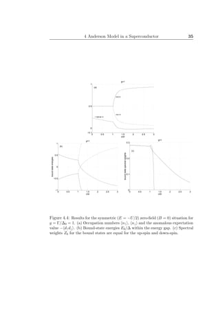
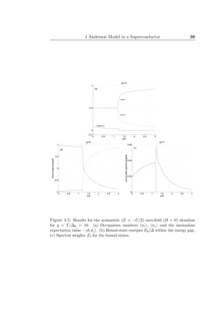
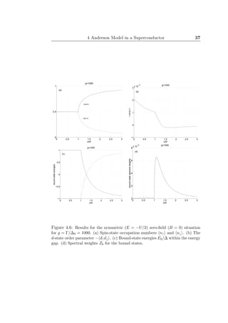
Figures 4.4, 4.5 and 4.6 show the results for the symmetric (E = −U/2)
zero-field (B = 0) situation for couplings Γ = ∆0, Γ = 10∆0 and Γ = 1000∆0,
respectively. A spontaneous symmetry breaking can be observed like in the

37. 4 Anderson Model in a Superconductor 34
case of a normal metal. In the magnetic regime, the bound-state energies
for spin up (σ = 1/2) decrease while the energies of spin-down bound states
increase with increasing local magnetic moment Sz = n↑ − n↓ . One of the
bound states for each of the spin directions merges into the continuum while
the other stays inside the gap. In the nonmagnetic regime, the bound-state
energies approach the gap center with decreasing coupling constant Γ, while
for larger couplings the bound states are found at the gap edge. Consequently,
Fig. 4.6c for large Γ is in exact agreement with Shiba’s results [21] and the
symmetry breaking occurs precisely at U = πΓ. One also observes that the d-
electron gap changes sign for large U but this takes place in the region where
the Hartree-Fock approximation is inapplicable. The nonmagnetic solution
nσ = n−σ exists also in the superconductor and it even seems to have a
nonvanishing region of convergence due to the third degree of freedom, aσ.
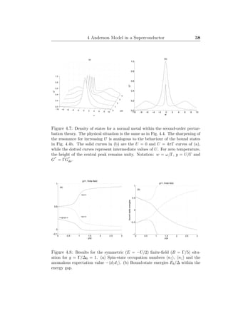
We see that the bound states tend towards the center of the gap for in-
creasing U until the HF approximation breaks down at U ≈ πΓ. Analogously,
if we consider the same physical situation as in Fig. 4.4 (∆0 = 1.76Tc ⇒
Γ/T = 1.76/0.2) for a normal metal to order U2
(see the previous chapter),
we observe that the zero-frequency Abrikosov-Suhl resonance sharpens as U
is increased. This is illustrated in Fig. 4.7.
Finite-field results are exemplified in Fig. 4.8 and an asymmetric situation
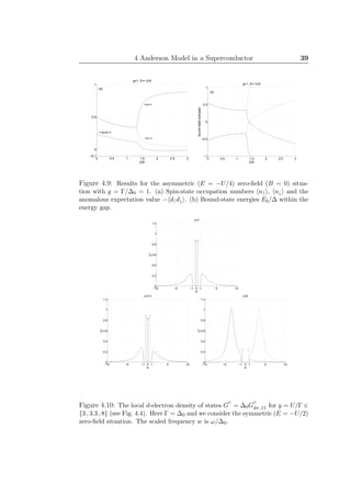
(E = −U/4) is considered in Fig. 4.9. For the spin-substate occupation
numbers the behaviour is similar to that found for a normal metal (Fig. 3.3).
For increasing asymmetry, the symmetry breaking occurs at a larger value of
U. Figure 4.10 shows the density of states in the physical situation of Fig.
4.4 for a few representative values of U.

38. 4 Anderson Model in a Superconductor 35
0 0.5 1 1.5 2 2.5 3
−0.1
0
0.5
1
y/pi
g=1
<n+>
<n−>
−<d+d−>
(a)
0 0.5 1 1.5 2 2.5 3
−1
−0.5
0
0.5
1
y/pi
boundstateenergies
g=1
(b)
0 0.5 1 1.5 2 2.5 3
0
0.1
0.2
0.3
y/pi
boundstatespectralweights
g=1
(c)
Figure 4.4: Results for the symmetric (E = −U/2) zero-field (B = 0) situation for
g = Γ/∆0 = 1. (a) Occupation numbers n↑ , n↓ and the anomalous expectation
value − d↑d↓ . (b) Bound-state energies Eb/∆ within the energy gap. (c) Spectral
weights Zb for the bound states are equal for the up-spin and down-spin.

39. 4 Anderson Model in a Superconductor 36
0 0.5 1 1.5 2 2.5 3
−0.1
0
0.5
1
y/pi
g=10
<n+>
<n−>
−<d+d−>
(a)
0 0.5 1 1.5 2 2.5 3
−1
−0.5
0
0.5
1
y/pi
boundstateenergies
g=10
(b)
0 0.5 1 1.5 2 2.5 3
0
0.02
0.04
0.06
y/pi
boundstatespectralweights
g=10
(c)
Figure 4.5: Results for the symmetric (E = −U/2) zero-field (B = 0) situation
for g = Γ/∆0 = 10. (a) Occupation numbers n↑ , n↓ and the anomalous
expectation value − d↑d↓ . (b) Bound-state energies Eb/∆ within the energy gap.
(c) Spectral weights Zb for the bound states.

40. 4 Anderson Model in a Superconductor 37
0 0.5 1 1.5 2 2.5 3
00
0.5
1
y/pi
g=1000
<n+>
<n−>
(a)
0 0.5 1 1.5 2 2.5 3
−1
0
1
2
3
x 10
−3
y/pi
−<d+d−>
g=1000
(b)
0 0.5 1 1.5 2 2.5 3
−1
−0.5
0
0.5
1
y/pi
boundstateenergies
g=1000
(c)
0 0.5 1 1.5 2 2.5 3
0
2
4
6
8
x 10
−4
y/pi
boundstatespectralweights
g=1000
(d)
Figure 4.6: Results for the symmetric (E = −U/2) zero-field (B = 0) situation
for g = Γ/∆0 = 1000. (a) Spin-state occupation numbers n↑ and n↓ . (b) The
d-state order parameter − d↑d↓ . (c) Bound-state energies Eb/∆ within the energy
gap. (d) Spectral weights Zb for the bound states.

41. 4 Anderson Model in a Superconductor 38
−10 −8 −6 −4 −2 0 2 4 6 8 10
0
1
2
3
4
0.0
0.2
0.4
0.6
0.8
1.0
w
G"
y/pi
(a)
−10 −8 −6 −4 −2 0 2 4 6 8 10
0.0
0.2
0.4
0.6
0.8
1.0
w
G"
(b)
Figure 4.7: Density of states for a normal metal within the second-order pertur-
bation theory. The physical situation is the same as in Fig. 4.4. The sharpening of
the resonance for increasing U is analogous to the behaviour of the bound states
in Fig. 4.4b. The solid curves in (b) are the U = 0 and U = 4πΓ curves of (a),
while the dotted curves represent intermediate values of U. For zero temperature,
the height of the central peak remains unity. Notation: w = ω/Γ, y = U/Γ and
G
′′
= ΓG
′′
dσ.
0 0.5 1 1.5 2 2.5 3
−0.1
0
0.5
1
y/pi
g=1, finite field
<n+>
<n−>−<d+d−>
(a)
0 0.5 1 1.5 2 2.5 3
−1
−0.5
0
0.5
1
y/pi
boundstateenergies
g=1, finite field
(b)
Figure 4.8: Results for the symmetric (E = −U/2) finite-field (B = Γ/5) situ-
ation for g = Γ/∆0 = 1. (a) Spin-state occupation numbers n↑ , n↓ and the
anomalous expectation value − d↑d↓ . (b) Bound-state energies Eb/∆ within the
energy gap.

42. 4 Anderson Model in a Superconductor 39
0 0.5 1 1.5 2 2.5 3
−0.1
0
0.5
1
y/pi
g=1, E=−U/4
<n+>
<n−>
−<d+d−>
(a)
0 0.5 1 1.5 2 2.5 3
−1
−0.5
0
0.5
1
y/pi
boundstateenergies
g=1, E=−U/4
(b)
Figure 4.9: Results for the asymmetric (E = −U/4) zero-field (B = 0) situa-
tion with g = Γ/∆0 = 1. (a) Spin-state occupation numbers n↑ , n↓ and the
anomalous expectation value − d↑d↓ . (b) Bound-state energies Eb/∆ within the
energy gap.
−10 −5 −1 0 1 5 10
0
0.2
0.4
0.6
0.8
1
1.2
w
G"
y=3
−10 −5 −1 0 1 5 10
0
0.2
0.4
0.6
0.8
1
1.2
w
G"
y=3.3
−10 −5 −1 0 1 5 10
0
0.2
0.4
0.6
0.8
1
1.2
w
G"
y=8
Figure 4.10: The local d-electron density of states G
′′
= ∆0G
′′
dσ ,11 for y = U/Γ ∈
{3 , 3.3 , 8} (see Fig. 4.4). Here Γ = ∆0 and we consider the symmetric (E = −U/2)
zero-field situation. The scaled frequency w is ω/∆0.

43. 4 Anderson Model in a Superconductor 40
4.4 Second-Order (U2
) Selfenergy Theory
As for the normal metal, we use the Hartree-Fock propagator (4.15) as the
vacuum state and express the T matrix as:
−Gdσ(z) = [Pσ(z) − Kσ(z) + Σσ(z)]−1
, (4.40)
where Pσ and Kσ are defined in Eqs. (4.16) and (4.17), respectively, and Σσ
is the selfenergy. In what follows, we obtain the selfenergy to the second
order in U. We relate the selfenergy to the HF propagator (4.37 a) which in
turn is a function of the parameters nσ , n−σ and aσ. These expectation
values are then obtained self-consistently using the propagator in Eq. (4.40).
4.4.1 Identification of the Selfenergy Σσ(ω)
The Hartree-Fock approximation (4.14) cuts the chain of equations of motion
for the components of the d-electron propagator Gdσ at the first level. Now
we surpass the HF approximation and apply the equations of motion one
step further. Consequently, we find:
−Gdσ = − G−1
mol + Kσ
−1
+ U G−1
mol + Kσ
−1
×
×
n−σ dσd−σ
dσd−σ nσ
+ U
1 0
0 −1
Σtrial ×
×
1 0
0 −1
G−1
mol + Kσ
−1
,
(4.41)
where we have defined:
Gmol = −
z − Eσ 0
0 z + E−σ
−1
(4.42)
and
Σtrial =
n−σdσ ; n−σd†
σ
+
n−σdσ ; nσd−σ
+
nσd†
−σ ; n−σd†
σ
+
nσd†
−σ ; nσd−σ
+ . (4.43)
Equation (4.41) is an analogue of Eq. (3.31). Now expanding the right-hand
side of Eq. (4.40) as in the normal-metal case leads us to identify the second-
order selfenergy:
Σσ(z) = −U2 1 0
0 −1
Σtrial
1 0
0 −1
= −U2 n−σdσ ; n−σd†
σ
+
z − n−σdσ ; nσd−σ
+
z
− nσd†
−σ ; n−σd†
σ
+
z nσd†
−σ ; nσd−σ
+
z
.
(4.44)

44. 4 Anderson Model in a Superconductor 41
The component Σ11σ is the familiar normal-metal term (3.32), while the
above structure is a Nambu-matrix generalization thereof.
4.4.2 Applying Wick’s Theorem
We proceed to evaluate the imaginary part of the selfenergy (4.44). Since
the calculation is similar for every component of Σσ we only show details for
the 11-component.
Using Eq. (A.10), we find:
Σ
′′
11σ =
U2
2
dt eiωt
d†
−σd−σdσ(t) d†
−σd−σd†
σ(0) + d†
−σd−σd†
σ(0) d†
−σd−σdσ(t) .
In the spirit of Wick’s theorem [40, 41, 59], we may now write (only the
nonzero contractions are shown):
Σ
′′
11σ =
U2
2
dt eiωt 1
d†
−σ
2
d−σ
3
dσ(t)
2
d†
−σ
1
d−σ
3
d†
σ(0) +
+
1
d†
−σ
2
d−σ
3
dσ(t)
2
d†
−σ
3
d−σ
1
d†
σ(0) +
+
1
d†
−σ
2
d−σ
3
d†
σ(0)
2
d†
−σ
1
d−σ
3
dσ(t) +
+
1
d†
−σ
2
d−σ
3
d†
σ(0)
3
d†
−σ
1
d−σ
2
dσ(t)
=
U2
2
dt eiωt
d−σ(t) d†
−σ(0) d†
−σ(t) d−σ(0) dσ(t) d†
σ(0) +
− d−σ(t) d†
−σ(0) dσ(t) d−σ(0) d†
−σ(t) d†
σ(0) +
+ d−σ(0) d†
−σ(t) d†
σ(0) dσ(t) d†
−σ(0) d−σ(t) +
− d−σ(0) dσ(t) d†
σ(0) d†
−σ(t) d†
−σ(0) d−σ(t) .
Above, operators with equal left upper indices are contracted. The two-
operator expectation values may now be calculated utilizing formulae (A.12),
which yield:
Σ
′′
11σ =
U2
2
dt eiωt dω1
π
e−iω1t dω2
π
e−iω2t dω3
π
e−iω3t
×
× {[1 − f(ω1)] [1 − f(ω2)] [1 − f(ω3)] + f(ω1)f(ω2)f(ω3)} ×
× G
′′
d−σd†
−σ
(ω1) G
′′
dσd†
σ
(ω2)G
′′
d†
−σd−σ
(ω3) − G
′′
dσd−σ
(ω2)G
′′
d†
−σd†
σ
(ω3) .

45. 4 Anderson Model in a Superconductor 42
Defining the propagators:
Gσ = Gdσd†
σ
(4.45 a)
Fσ = Gdσd−σ (4.45 b)
Fσ = Gd†
−σd†
σ
(4.45 c)
Gσ = Gd†
−σd−σ
(4.45 d)
and an integral operator:
ˆF =
U2
2
dt
dω1
π
dω2
π
dω3
π
eit(ω−ω1−ω2−ω3)
×
× {[1 − f(ω1)] [1 − f(ω2)] [1 − f(ω3)] + f(ω1)f(ω2)f(ω3)}
=U2 dω1
π
dω2
π
dω3 δ(ω − ω1 − ω2 − ω3)×
× {[1 − f(ω1)] [1 − f(ω2)] [1 − f(ω3)] + f(ω1)f(ω2)f(ω3)}
(4.46)
we may write Σ
′′
11σ in a shorthand form:
Σ
′′
11σ = ˆF G
′′
−σ G
′′
σG
′′
σ − F
′′
σ F
′′
σ . (4.47)
Formula (3.33) was used in Eq. (4.46).
Performing a similar calculation for the remaining three components of
Σσ we straightforwardly obtain:



Σ
′′
11σ(ω) = ˆF G
′′
−σ G
′′
σG
′′
σ − F
′′
σ F
′′
σ
Σ
′′
12σ(ω) = − ˆF F
′′
−σ G
′′
σG
′′
σ − F
′′
σ F
′′
σ
Σ
′′
21σ(ω) = − ˆF F
′′
−σ G
′′
σG
′′
σ − F
′′
σ F
′′
σ
Σ
′′
22σ(ω) = ˆF G
′′
−σ G
′′
σG
′′
σ − F
′′
σ F
′′
σ .
(4.48)
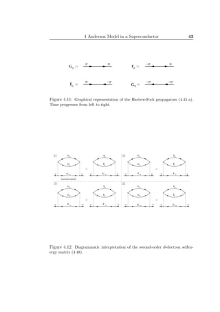
The Green’s functions (4.45 a) are represented diagrammatically in Fig. 4.11.
Consequently, we find that the selfenergy is now composed of the diagrams
shown in Fig. 4.12. We observe that the selfenergy in a normal metal only
has the first of the graphs of Σ11σ (see Fig. 3.4).
If the Green’s function were to be determined selfconsistently, the propa-
gators Gσ, Gσ, Fσ and Fσ on the right-hand side of Eq. (4.48) would be given
by Eq. (4.40). However, we determine only the parameters nσ , n−σ and
aσ selfconsistently and therefore use the Hartree-Fock result (4.37 b) for the
propagators (4.45 d). Consequently, in the following it is understood that
the symbols Gσ, Gσ, Fσ and Fσ in the selfenergy always stand for the HF
propagators.

46. 4 Anderson Model in a Superconductor 43
Fs
Fs
Gs
Gs
s s
s s
ss
s s
Figure 4.11: Graphical representation of the Hartree-Fock propagators (4.45 a).
Time progresses from left to right.
s s s sG s
Gs
Gs Fs
Fs Gs
Gs Fs
Fs
Gs
Gs Fs
Fs Gs
Gs Fs
Fs
11 12
21 22
G s F ss s F ss s
G s ss G s sssF ss sF ss
(normal metal)
Figure 4.12: Diagrammatic interpretation of the second-order d-electron selfen-
ergy matrix (4.48).

47. 4 Anderson Model in a Superconductor 44
4.4.3 Formulation in the Time Domain
As in the normal-metal case, we may utilize the spectral representation (A.5)
in order to obtain the entire function Σσ(z) defined in the complex plane from
the imaginary part Σ
′′
σ(ω) (4.48), where ω is a real frequency. Consequently,
the multidimensional integrals can be written in terms of one-dimensional
Fourier integrals with the help of Eq. (3.36) as follows:
Define:
A>
σ (λ) =
∞
−∞
dω
π
e−iλω
[1 − f(ω)] G
′′
σ(ω) (4.49 a)
A
>
σ (λ) =
∞
−∞
dω
π
e−iλω
[1 − f(ω)] G
′′
σ(ω) (4.49 b)
A<
σ (λ) =
∞
−∞
dω
π
e−iλω
f(ω)G
′′
σ(ω) (4.49 c)
A
<
σ (λ) =
∞
−∞
dω
π
e−iλω
f(ω)G
′′
σ(ω) (4.49 d)
B>
σ (λ) =
∞
−∞
dω
π
e−iλω
[1 − f(ω)] F
′′
σ (ω) (4.49 e)
B
>
σ (λ) =
∞
−∞
dω
π
e−iλω
[1 − f(ω)] F
′′
σ(ω) (4.49 f)
B<
σ (λ) =
∞
−∞
dω
π
e−iλω
f(ω)F
′′
σ (ω) (4.49 g)
B
<
σ (λ) =
∞
−∞
dω
π
e−iλω
f(ω)F
′′
σ(ω) (4.49 h)
and
C>
σ (λ) = A>
σ A
>
σ − B>
σ B
>
σ (4.50 a)
C<
σ (λ) = A<
σ A
<
σ − B<
σ B
<
σ . (4.50 b)
The selfenergy may then be expressed as:



Σ11σ(z) = iU2
∞
0
dλ eiλz
A>
−σ(λ)C>
σ (λ) + A<
−σ(λ)C<
σ (λ)
Σ12σ(z) = −iU2
∞
0
dλ eiλz
B>
−σ(λ)C>
σ (λ) + B<
−σ(λ)C<
σ (λ)
Σ21σ(z) = −iU2
∞
0
dλ eiλz
B
>
−σ(λ)C>
σ (λ) + B
<
−σ(λ)C<
σ (λ)
Σ22σ(z) = iU2
∞
0
dλ eiλz
A
>
−σ(λ)C>
σ (λ) + A
<
−σ(λ)C<
σ (λ) .
(4.51)

48. 4 Anderson Model in a Superconductor 45
The Hartree-Fock propagator (previous section) enters here on the right-hand
side of Eqs. (4.49 c).
The above result (4.51) looks deceivingly simple and appealing. However,
the delta-function parts of the HF propagators (4.29 a) yield constant con-
tributions to A≷
σ , A
≷
σ , B≷
σ and B
≷
σ which, in turn, causes the selfenergy to
possess delta-function components. These delta-function peaks in the self-
energy cannot be computed numerically starting from Eqs. (4.51). Instead,
they must be obtained analytically which proves to be a tedious calculation.
Equations (4.51) may be somewhat simplified by noting the following
symmetries:
A
≷
σ (λ) = A≶∗
−σ(λ) (4.52 a)
B
≷
σ (λ) = B≶∗
−σ(λ) (4.52 b)
B
≷
σ = B≷
σ . (4.52 c)
The equality (4.52 c c) follows from the fact that, in general:
Fσ = Fσ. (4.53)
Consequently, we find that the selfenergy displays the following symmetry
properties:
−Σ∗
11−σ(−ω) = Σ22σ(ω) (4.54 a)
−Σ∗
12−σ(−ω) = Σ21σ(ω) (4.54 b)
−Σ∗
21−σ(−ω) = Σ12σ(ω) (4.54 c)
−Σ∗
22−σ(−ω) = Σ11σ(ω) (4.54 d)
which are the same as those obeyed by Kij in Eq. (4.24 a) (note that K11 =
K22 and K12 = K21).
Up to this point we have not made any restrictions on the physical situ-
ation under consideration. However, in the following we restrict ourselves to
discuss only the most interesting symmetric (E = −U/2) zero-field (B = 0)
case. Due to the particle-hole symmetry, this assumption simplifies the ensu-
ing calculations a great deal. In particular, we may set nσ = n−σ = 1/2
which gives (actually nσ = n−σ = 1/2 is an assumption that was proved
to be valid for normal metal and will later be shown to be selfconsistent for
the superconductor as well):
Gσ = Gσ (4.55 a)
Gσ = G−σ (4.55 b)
Fσ = −F−σ (4.55 c)

49. 4 Anderson Model in a Superconductor 46
implying
A
≷
σ = A≷
σ (4.56 a)
A≷
σ = A≷
−σ (4.56 b)
B≷
σ = −B≷
−σ. (4.56 c)
Consequently, we now find for the selfenergy:



Σ11σ(z) = iU2
∞
0
dλ eiλz
[A>
σ (λ)C>
σ (λ) + A<
σ (λ)C<
σ (λ)]
Σ12σ(z) = iU2
∞
0
dλ eiλz
[B>
σ (λ)C>
σ (λ) + B<
σ (λ)C<
σ (λ)]
Σ21σ(z) = Σ12σ(z)
Σ22σ(z) = Σ11σ(z),
(4.57)
where
C≷
σ = A≷
σ
2
− B≷
σ
2
. (4.58)
Thus, we find that only the 11- and 12-components of the selfenergy are
independent. Moreover, we may consider only one of the spin components.
By inspecting the Hartree-Fock equations (previous section), we find that
when the occupation numbers are set to their correct values nσ = n−σ =
1/2, we have two bound states Eb+ and Eb− that do not depend on the spin
direction. These bound states reside symmetrically with respect to the Fermi
level, such that Eb− = −Eb+
def
= −Eb < 0 and for the spectral weights of the
diagonal terms we find Zb− = Zb+
def
= Zb and Qb− = −Qb+
def
= −Qb for the
off-diagonal terms. Furthermore, it is easily demonstrated that Q2
b = Z2
b .
To enable fully utilizing the symmetry and in order to extract the delta-
function contributions in the selfenergy, we write our formulae in terms of
the symmetrized and antisymmetrized linear combinations of A≷
σ and B≷
σ :
A+
σ = A>
σ + A<
σ (4.59 a)
A−
σ = A>
σ − A<
σ (4.59 b)
B+
σ = B>
σ + B<
σ (4.59 c)
B−
σ = B>
σ − B<
σ . (4.59 d)

50. 4 Anderson Model in a Superconductor 47
In this way, we obtain after tedious algebra:



Σ11
ω
∆
=i
U2
∆
∞
0
dl eilω/∆
R(l) −
U2
∆
Z3
b
vb
1 − tanh2 vbαβ
2
ω
∆
×
× P
1
ω
∆
− vb
−
1
ω
∆
+ vb
− iπ δ(
ω
∆
− vb) − δ(
ω
∆
+ vb)
Σ12
ω
∆
=
U2
∆
∞
0
dl eilω/∆
P(l) −
U2
∆
Q3
b 1 − tanh2 vbαβ
2
×
× P
1
ω
∆
− vb
−
1
ω
∆
+ vb
− iπ δ(
ω
∆
− vb) − δ(
ω
∆
+ vb) ,
(4.60)
where
l = λ∆; vb =
Eb
∆
; α =
∆
Γ
; β =
Γ
T
(4.61)
define the dimensionless parameters l, vb, α and β,
R(l)
2
= I+
A I+
A
2
− 3 I−
A
2
+ I+
B
2
− I−
B
2
+
+2Z2
b 1 − tanh2 vbαβ
2
+ 2I−
A I+
B I−
B +
+ cos (lvb) Zb 3 I+
A
2
− 3 I−
A
2
+ I+
B
2
− I−
B
2
+
−2Qbtanh
vbαβ
2
I+
A I−
B − I−
A I+
B +
+ sin (lvb) 2Qb I+
A I+
B + I−
A I−
B − 2Zbtanh
vbαβ
2
3I+
A I−
A − I+
B I−
B +
+ cos (2lvb) Z2
b 1 + tanh2 vbαβ
2
I+
A − 2ZbQbtanh
vbαβ
2
I−
B
+ sin (2lvb) ZbQb 1 + tanh2 vbαβ
2
I+
B − 2Z2
b tanh
vbαβ
2
I−
A (4.62)

51. 4 Anderson Model in a Superconductor 48
and
P(l)
2
= I+
B I+
B
2
− 3 I−
B
2
+ I+
A
2
− I−
A
2
+
+2Q2
b 1 − tanh2 vbαβ
2
+ 2I+
A I−
A I−
B +
+ cos (lvb) 2Zb I+
A I+
B + I−
A I−
B − 2Qbtanh
vbαβ
2
3I+
B I−
B − I+
A I−
A +
+ sin (lvb) Qb 3 I+
B
2
− 3 I−
B
2
+ I+
A
2
− I−
A
2
+
−2Zbtanh
vbαβ
2
I−
A I+
B − I+
A I−
B +
+ cos (2lvb) 2ZbQbtanh
vbαβ
2
I−
A − Q2
b 1 + tanh2 vbαβ
2
I+
B
+ sin (2lvb) ZbQb 1 + tanh2 vbαβ
2
I+
A − 2Q2
btanh
vbαβ
2
I−
B . (4.63)
The following abbreviations were introduced above:
I+
A =
∞
1
dv
π
cos (lv) ∆A(ω) (4.64 a)
I−
A =
∞
1
dv
π
sin (lv) tanh
vαβ
2
∆A(ω) (4.64 b)
I+
B =
∞
1
dv
π
sin (lv) ∆C(ω) (4.64 c)
I−
B =
∞
1
dv
π
cos (lv) tanh
vαβ
2
∆C(ω). (4.64 d)
Here v = ω/∆, while A(ω) and C(ω) are the continuum parts of the diago-
nal and off-diagonal Hartree-Fock spectral densities, Eqs. (4.34) and (4.35),
respectively.
From the result (4.60) one finds that the selfenergy displays the same
symmetry properties as Kij (4.18):
−Σ∗
11(−ω) = Σ11(ω)
Σ∗
12(−ω) = Σ12(ω).
(4.65)
Furthermore, we observe that R(l) is symmetric, while P(l) is an antisym-
metric function.

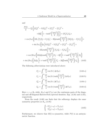
52. 4 Anderson Model in a Superconductor 49
The bound states, spectral weights and the d-state order parameter − d↑d↓
are now to be determined selfconsistently beyond the Hartree-Fock theory
using the second-order propagator in Eq. (4.40). Utilizing the symmetries
(4.65) and those of Kij, one can again show that the bound states are situ-
ated symmetrically with respect to the Fermi level. Moreover, using formulae
(4.54 a) we observe that the symmetries (4.25 a) are valid for the d-electron
Green’s function also within the U2
perturbation theory. Consequently, as
above, we conclude that the d-state gap aσ is real.
Although the time-domain formulation allows one to easily establish the
symmetries obeyed by the selfenergy and the T matrix up to second order
in U, the numerical evaluation of Eqs. (4.60) becomes overly cumbersome.
Since the lower integration limit in Eq. (4.64 a) is unity, the functions I±
A
and I±
B oscillate nonperiodically and for large values of l they die off not
faster than 1/l2
. This behaviour is carried over to the functions R(l) and
P(l). Consequently, we were not able to compute the Fourier transforms of
R(l) and P(l) in Eq. (4.48) efficiently enough. Owing to these difficulties, we
chose to perform the calculations in the frequency domain, without Fourier
integrals as explained in what follows.
4.4.4 Formulation in the Frequency Domain for the
Symmetric Zero-Field Situation
It has proven that the optimal way of accomplishing the analytical and nu-
merical calculations is to insert the Hartree-Fock propagators directly into
Eq. (4.48) for the imaginary part of the selfenergy. The real part is there-
after found by utilizing Eq. (A.8). Noting also that for the HF propagators
(4.45 d) G
′′
σ = G
′′
−σ and F
′′
σ = −F
′′
−σ, we obtain after fair amount of work:



Σ
′′
11σ(ω) =
U2
π2
[I−1 + I0 + I1 + I2]
Σ
′′
12σ(ω) =
U2
π2
[J−1 + J0 + J1 + J2] ,
(4.66)
where
I−1 = 4π3
Z3
b f(Eb)[1−f(Eb)][δ(ω−Eb)+δ(ω+Eb)], (4.67)
I0 =8π2
Z2
b
˜A(ω) ˜f(Eb, ω, ω) + 2π2
Z2
b
˜A(ω − 2Eb) ˜f(Eb, Eb, ω)+
+ 2π2
Z2
b
˜A(ω + 2Eb) ˜f(−Eb, −Eb, ω)+
+ 2π2
ZbQb
˜C(ω + 2Eb) ˜f(−Eb, −Eb, ω)+
− 2π2
ZbQb
˜C(ω − 2Eb) ˜f(Eb, Eb, ω),
(4.68)

53. 4 Anderson Model in a Superconductor 50
I1 =3πZb dω1
˜A(ω1) ˜A(ω − ω1 − Eb) ˜f(Eb, ω1, ω)+
+ 3πZb dω1
˜A(ω1) ˜A(ω − ω1 + Eb) ˜f(−Eb, ω1, ω)+
+ 2πQb dω1
˜A(ω1) ˜C(ω − ω1 + Eb) ˜f(−Eb, ω1, ω)+
− 2πQb dω1
˜A(ω1) ˜C(ω − ω1 − Eb) ˜f(Eb, ω1, ω)+
− πZb dω1
˜C(ω1) ˜C(ω − ω1 − Eb) ˜f(Eb, ω1, ω)+
− πZb dω1
˜C(ω1) ˜C(ω − ω1 + Eb) ˜f(−Eb, ω1, ω),
(4.69)
I2 = dω1 dω2
˜f(ω1, ω2, ω) ˜A(ω1) ˜A(ω2) ˜A(ω − ω1 − ω2)+
− ˜C(ω2) ˜C(ω − ω1 − ω2) ,
(4.70)
J−1 = 4π3
Q3
bf(Eb)[1−f(Eb)][δ(ω−Eb)−δ(ω+Eb)], (4.71)
J0 =8π2
Z2
b
˜C(ω) ˜f(Eb, ω, ω) − 2π2
Z2
b
˜C(ω − 2Eb) ˜f(Eb, Eb, ω)+
− 2π2
Z2
b
˜C(ω + 2Eb) ˜f(−Eb, −Eb, ω)+
− 2π2
ZbQb
˜A(ω + 2Eb) ˜f(−Eb, −Eb, ω)+
+ 2π2
ZbQb
˜A(ω − 2Eb) ˜f(Eb, Eb, ω),
(4.72)
J1 = − 3πQb dω1
˜C(ω1) ˜C(ω − ω1 − Eb) ˜f(Eb, ω1, ω)+
+ 3πQb dω1
˜C(ω1) ˜C(ω − ω1 + Eb) ˜f(−Eb, ω1, ω)+
+ 2πZb dω1
˜C(ω1) ˜A(ω − ω1 + Eb) ˜f(−Eb, ω1, ω)+
+ 2πZb dω1
˜C(ω1) ˜A(ω − ω1 − Eb) ˜f(Eb, ω1, ω)+
+ πQb dω1
˜A(ω1) ˜A(ω − ω1 − Eb) ˜f(Eb, ω1, ω)+
− πQb dω1
˜A(ω1) ˜A(ω − ω1 + Eb) ˜f(−Eb, ω1, ω),
(4.73)
J2 = dω1 dω2
˜f(ω1, ω2, ω) ˜C(ω1) ˜A(ω2) ˜A(ω − ω1 − ω2)+
− ˜C(ω2) ˜C(ω − ω1 − ω2) ,
(4.74)

54. 4 Anderson Model in a Superconductor 51
˜f(ω1, ω2, ω3) = [1−f(ω1)] [1−f(ω2)] [1−f(ω3)]+f(ω1)f(ω2)f(ω3), (4.75)
˜A(ω) = A(ω)θ(ω2
− ∆2
) (4.76)
and
˜C(ω) = C(ω)θ(ω2
− ∆2
). (4.77)
Here f is the Fermi distribution (A.13), θ is the Heaviside step function and
δ denotes the Dirac delta function. A(ω) and C(ω) are the continuum parts
of the Hartree-Fock spectral densities (4.34) and (4.35), respectively. The
delta-function parts of the selfenergy (I−1 and J−1) can easily be seen to
agree with our previous result (4.60). In obtaining the real parts using Eq.
(A.8), the symmetries (4.65) can be employed to convert the integral to one
over positive frequencies only.
It is interesting to notice that all the discontinuities of the selfenergy re-
side in the terms I0 and J0 which contain no integrals. This is what makes
the frequency-domain formulation superior to our earlier attempt in the time
domain. The numerical routines that we utilize to calculate the Fourier in-
tegrals in Eq. (4.60) failed at the discontinuities. Thus, the time-domain
formulation could perhaps be developed further by extracting the discontin-
uous parts of the integrals in Eq. (4.60) by hand.
In spite of the fact that I0 and J0 have terms containing θ(ω + 2Eb), the
imaginary part of Σ will be seen to vanish inside the energy gap. This sim-
plifies the analysis of the bound-state spectrum in the following subsection.
Furthermore, the double integrals I2 and J2 are much smaller than the other
components and may be neglected, to the first approximation. However, we
will in fact approximate I2 and J2 and verify that their contribution to the
final result indeed is neglible.
4.4.5 Density of States and the Selfconsistency Condi-
tion
The d-electron propagator (4.40) may be written as:
ˆGdσ = −
1
ˆDσ
z−K11σ +Σ11σ −U dσd−σ +K12σ −Σ12σ
−U dσd−σ +K12σ −Σ12σ z−K11σ +Σ11σ
.(4.78)
Here we have used K11 = K22, K21 = K12, Σ11 = Σ22, Σ21 = Σ12 and
substituted E = −U/2 and nσ = n−σ = 1/2. The determinant is now:
ˆDσ(z) = Dσ(z) + 2Σ11(z − K11) − 2Σ12(Uaσ − K12) + Σ2
11 − Σ2
12, (4.79)

55. 4 Anderson Model in a Superconductor 52
where Dσ is the Hartree-Fock term (4.23). In what follows, we choose to write
the equations using nondimensional parameters α and β (4.61), v = ω/∆,
y = U/Γ, x = E/Γ and S = ∆Σ/(U2
). Furthermore, symbols with a caret,
such as ˆDσ, denote the second-order results while symbols without the caret,
such as Dσ, refer to the Hartree-Fock approximation.
Bound States in the Gap (|ω| < ∆)
Within the energy gap (|v| < 1), we obtain for the determinant:
α2 ˆDσ
∆2
=
α2
Dσ
∆2
+ 2vy2
1 +
1
α
√
1 − v2
S
′
11+
−
2y2
α
aσy +
1
√
1 − v2
S
′
12 +
y4
α2
S
′
11
2
− S
′
12
2
.
(4.80)
Also the derivative ˆD
′
σ of the determinant with respect to frequency is needed:
α ˆD
′
σ
∆
=
αD
′
σ
∆
+
1
α
2y2
1 +
1
α
√
1 − v2
S
′
11 + v
dS
′
11
dv
+
+
2y2
v
α(1 − v2)
√
1 − v2
vS
′
11 − S
′
12 +
−
2y2
α
aσy+
1
√
1 − v2
dS
′
12
dv
+
y4
α2
2S
′
11
dS
′
11
dv
−2S
′
12
dS
′
12
dv
.
(4.81)
The bound states ˆvb, to the second order in U, are now the zeros of the
determinant (4.80) and the corresponding diagonal and off-diagonal spectral
weights are found as above for the HF approximation:
ˆZb =
αˆvb +
ˆvb
1 − ˆv2
b
+
y2
α
S
′
11(ˆvb)
α ˆD′
σ/∆
(4.82 a)
ˆQb = −
yaσ +
2σ
1 − ˆv2
b
+
y2
α
S
′
12(ˆvb)
α ˆD′
σ/∆
. (4.82 b)
The bound states are situated symmetrically with respect to the Fermi level.
Moreover, we find that ˆZb(ˆvb) = ˆZb(−ˆvb) and ˆQb(ˆvb) = − ˆQb(−ˆvb). Thus it
suffices to consider positive frequencies only.

56. 4 Anderson Model in a Superconductor 53
Continuum Contributions (|ω| > ∆)
Beyond the gap edge (|v| > 1), we find for the determinant (4.79):
ˆDσ
∆2
=
ℜ ˆDσ
∆2
+ i
ℑ ˆDσ
∆2
, (4.83 a)
where the real (ℜ) and imaginary (ℑ) parts equal:
ℜ ˆDσ
∆2
=
ℜDσ
∆2
+
2vy2
α2
S
′
11 −
2y2
α2
|v|
α
√
v2 − 1
S
′′
11 −
2aσy3
α3
S
′
12+
+
2y2
α2
2σsgn(v)
α
√
v2 − 1
S
′′
12+
+
y4
α4
S
′
11
2
− S
′′
11
2
− S
′
12
2
+ S
′′
12
2
(4.83 b)
and
ℑ ˆDσ
∆2
=
ℑDσ
∆2
+
2vy2
α2
S
′′
11 +
2y2
α2
|v|
α
√
v2 − 1
S
′
11 −
2aσy3
α3
S
′′
12+
−
2y2
α2
2σsgn(v)
α
√
v2 − 1
S
′
12 + 2
y4
α4
S
′
11S
′′
11 − S
′
12S
′′
12 .
(4.83 c)
Consequently, we find the continuum parts ˆA and ˆC of the diagonal and
off-diagonal spectral densities, respectively:
∆ ˆA = −
1
ℜDσ
∆2
2
+ ℑDσ
∆2
2
ℜDσ
∆2
|v|
α
√
v2 − 1
+
y2
α2
S
′′
11 +
−
ℑDσ
∆2
v +
y2
α2
S
′
11
(4.84)
and
∆ ˆC =
1
ℜDσ
∆2
2
+ ℑDσ
∆2
2
ℜDσ
∆2
sgn(v)
α
√
v2 − 1
+
y2
α2
S
′′
12 +
−
ℑDσ
∆2
aσy
α
+
y2
α2
S
′
12 .
(4.85)
Thus, the imaginary parts of the 11- and 12-components of the d-electron
Green’s function are given by (similarly to Eq. (4.37 b)):
∆ ˆG
′′
11σ = π
b
ˆZb δ(v − ˆvb) + ∆ ˆA θ(v2
− 1) (4.86 a)
∆ ˆG
′′
12σ = π
b
ˆQb δ(v − ˆvb) + ∆ ˆC θ(v2
− 1). (4.86 b)

57. 4 Anderson Model in a Superconductor 54
It is interesting to note that - just as in the Hartree-Fock approximation -
G
′′
11 is symmetric while G
′′
12 is an antisymmetric function of frequency.
The Selfconsistency Condition and the Diagonal Sum Rule
Equation (A.12) gives us now the selfconsistency condition for the d-state
order parameter:
aσ =
∞
−∞
dω
2π
tanh
ω
2T
G
′′
12σ(ω)
=
b ,vb>0
ˆQb tanh
ˆvbαβ
2
+
∞
1
dv
π
tanh
vαβ
2
∆ ˆC.
(4.87)
Furthermore, since in zero field nσ = n−σ is obeyed, the numerical value
nσ = n−σ = 1/2 follows from the diagonal sum rule (see Eq. (4.36)):
1 =
∞
−∞
dω
π
ˆG
′′
11σ(ω). (4.88)
In computing the numerical results, the above sum rule was always checked
to be satisfied by the density of states ˆG
′′
11. Due to the fact that the second-
order calculation is much more complicated than the HF case, we chose for
the relative accuracy of the final results 10−3
.

58. Chapter 5
Numerical Results
We now consider the physical situation in Fig. 4.4 (especially, Γ = ∆0 and
T = 0.2Tc) and compare the second-order selfenergy calculations to those
obtained using the Hartree-Fock approximation.
Figure 5.1 shows the continuum components I0,1,2 and J0,1,2 of the self-
energy in Eq. (4.66) for a representative value of U, namely U = 6Γ. We
find that the two-dimensional integrals I2 and J2 grow comparable to the
other components only for relatively large frequencies. This suggests that we
may ignore I2 and J2 in considering the density of states and thus save a fair
amount of CPU-time. This point will be further justified below.
Figures 5.2 and 5.3 show the results for energies and spectral weights of
the spin-degenerate bound states for positive frequencies (we consider the
symmetric situation). The dashed line is the Hartree-Fock result in the non-
magnetic regime (see Fig. 4.4(b and c)). The most important point to notice
is that we now have two separate bound states (E1 and E2) also in the
small-U limit, while the HF approximation scheme only results in a single
bound state (EHF). The HF bound state is the average of the two new bound
states (EHF = (E1 + E2)/2). We also observe that the sum of the spectral
weights of the new bound states equals the HF weight in the small-U limit
(ZHF = Z1 + Z2). Furthermore, we find a level crossing in the localized state
marked E1 approximately at U = 7.6Γ. The circles denote results when the
two-dimensional integrals I2 and J2 are taken into account. Thus, one sees
that I2 and J2 can indeed be neglected.
The anomalous expectation value − d↑d↓ is shown in Fig. 5.4. The
Hartree-Fock result (dashed line) is seen to be correct in the small-U limit.
As pointed out earlier, the d-state gap changes sign for increasing U.
Figures 5.5, 5.6 and 5.7 display the d-electron density of states and
the continuous component of the imaginary part of the diagonal selfenergy
Σ11(ω). As in the normal-metal case, we have an accumulation of spectral

59. 5 Numerical Results 56
0 1 2 4 6 8 10
0
0.01
0.02
0.03
0.04
0.05
v
y=6
0 1 2 4 6 8 10
−0.05
−0.04
−0.03
−0.02
−0.01
0
0.01
v
y=6
Figure 5.1: Continuum components I0,1,2 and J0,1,2 of the diagonal (left) and
off-diagonal (right) selfenergy, Eq. (4.66), in units of π2/∆. Here y = U/Γ = 6
and v = ω/∆ as usual. (solid line): I0 Eq. (4.68) and J0 Eq. (4.72). (dashed line):
I1 Eq. (4.69) and J1 Eq. (4.73). (dotted line): I2 Eq. (4.70) and J2 Eq. (4.74).
weight in the center of the gap and broad resonances approximately at ener-
gies ω = ±U/2. In addition, we have a small dip at the discontinuity of the
selfenergy which occurs precisely for ω = ∆ + 2EHF. However, it is too early
to suggest to what physical process this dip is related to since this research
continues.

60. 5 Numerical Results 57
0 2 4 6 8 10 12
0
0.1
0.2
0.3
0.4
0.5
0.6
0.7
0.8
0.9
1
y
boundstateenergies
E1
E2
EHF
(E1 + E2)/2
Figure 5.2: Bound-state energies Eb/∆ within the energy gap. (solid line, E1
and E2): Second-order results. The two-dimensional integrals I2 and J2 are taken
into account at the points marked with the circles. (dashed line, EHF): The single
Hartree-Fock bound state. (dotted line): (E1 + E2)/2.
0 2 4 6 8 10 12
0
0.05
0.1
0.15
0.2
0.25
0.3
y
boundstatespectralweights
Z2
Z1
(Z1 + Z2)
ZHF
Figure 5.3: Spectral weights for the bound states. (solid line, Z1 and Z2): Second-
order results. The two-dimensional integrals I2 and J2 are taken into account at
the points marked with the circles. (dashed line, ZHF): The Hartree-Fock spectral
weight. (dotted line): (Z1 + Z2).

61. 5 Numerical Results 58
0 2 4 6 8 10 12
−0.1
0
0.1
0.2
0.25
y
−<d+d−>
Figure 5.4: The d-state order parameter − d↑d↓ . The two-dimensional integrals
I2 and J2 are taken into account at the points marked with the circles. The dashed
line represents the HF result.
0 1 2 3 4 6 8 10
0
0.1
0.2
0.3
0.4
0.5
0.6
0.7
v
y=2
Figure 5.5: Density of states in units of 1/∆ (solid line) and the continuous
component of the imaginary part of the diagonal selfenergy in units of U2/∆
(dashed line) for y = U/Γ = 2. Horizontal axis: v = ω/∆.

62. 5 Numerical Results 59
0 1 2 3 4 6 8 10
0
0.1
0.2
0.3
0.4
0.5
0.6
0.7
v
y=7
Figure 5.6: As in Fig. 5.5, but for y = U/Γ = 7.
0 1 2 3 4 6 8 10
0
0.1
0.2
0.3
0.4
0.5
0.6
0.7
v
y=12
Figure 5.7: As in Fig. 5.5, but for y = U/Γ = 12.

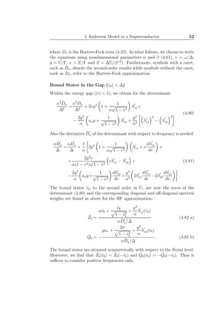
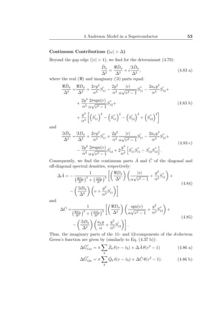
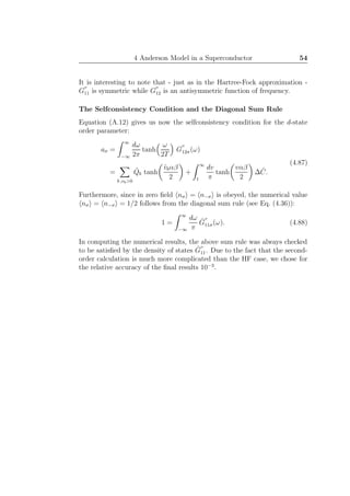
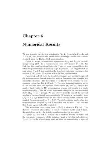
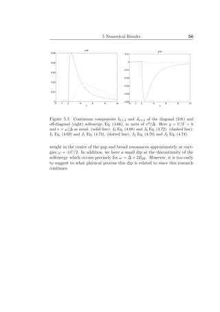
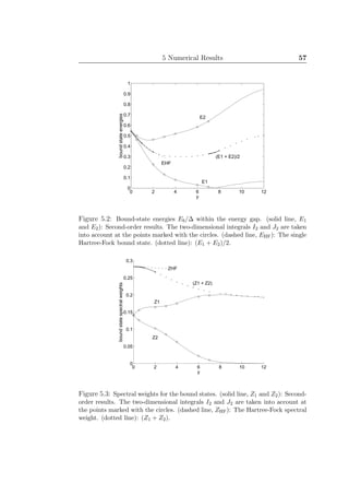
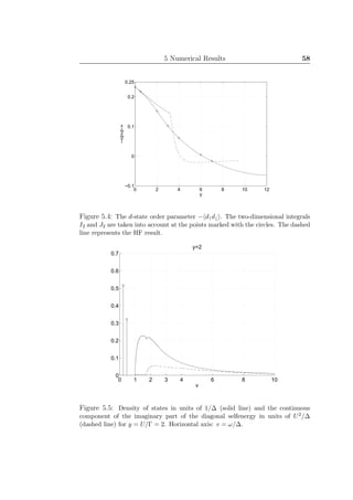
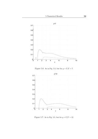
63. Chapter 6
Discussion
We have generalized the selfenergy theory for the Anderson model from a
normal-metal host to the case of a BCS superconductor. We have demon-
strated that spin fluctuations and pairing fluctuations both contribute to the
selfenergy structure. Even in the small-U limit, the second-order theory is
shown to give a physical picture that differs considerably from that of the
Hartree-Fock approximation. Especially, new bound states within the en-
ergy gap are found and their relation to the localized states found within
the HF theory is thoroughly investigated. The triple-peaked structure of the
d-electron density of states for the normal metal in the strong-correlation
regime [33] is in this work shown to have its analogue in a BCS superconduc-
tor. We have demonstrated an accumulation of spectral weight at the gap
center in the superconductor as the interatomic Coulomb-repulsion energy U
is increased. Furthermore, broad side resonances related to the eigenstates
of the atomic limit (Section 2.1) are found as in the normal-metal case.
The Anderson model was originally proposed for the study of the magnetic-
nonmagnetic transition in normal metals. The Hartree-Fock calculation sug-
gests an abrupt phase transition originating from a spontaneous symmetry
breaking in the occupation numbers of the localized state as the interatomic
Coulomb-repulsion energy is increased. However, since we are dealing with a
microscopic system which is localized in real space around the impurity, the
passage from a magnetic behaviour to a nonmagnetic behaviour cannot be a
true phase transition. A true phase transition needs a macroscopic system,
and it is in the limit of an infinite system that the theoretical quantities of
interest do show mathematical singularities. Thus the M-NM transition for
an impurity should be a gradual transition which does not exhibit critical
properties (a critical value of the parameter Γ/U, for example). The second-
order (U2
) treatment removes this unphysical symmetry breaking and gives a
smooth magnetic-nonmagnetic transition. This is seen, for example, by con-

64. 6 Discussion 61
sidering the magnetic susceptibility that approaches the Curie law for large
U. We expect that the second-order selfenergy theory for a superconductor,
presented for the first time in this work, will prove out to be at least of equal
importance as the normal-metal result.
The behaviour of the local electron, especially the d-electron density of
states, can be probed by a large number of spectroscopies [60]. In valence
photoemission (VP), the absorbtion of a photon excites a local electron to
a high kinetic energy. Some of these energetic electrons escape from the
surface of the sample, and are analyzed. Usually it is assumed that the
energetic electron does not scatter during its departure from the surface. If it
does interact, it usually changes its energy significantly and is not detected.
Valence photoemission is used to measure the occupied density of states
below the Fermi surface (negative energies). The unoccupied DOS (positive
energies) can be measured using Bremsstrahlung isochromat spectroscopy
(BIS). Here an electron of high energy is shot at the solid. It can emit a
photon while falling into a lower-energy electron state. The photon-emission
rate is then measured. In a superconductor there is an energy gap ∆ in the
excitation spectrum. This must be taken into account in the spectroscopies.
For example, the energy of the initial photon in VP must be larger than
2∆ in order to break Cooper pairs. Also in a real sample, there is a finite
concentration of impurities. This causes the bound states within the energy
gap to appear not as delta-function peaks but rather as impurity bands of
finite width.
There are also suggestions that the Anderson model is insufficient for
the discussion of heavy fermions (for a review of heavy fermions see, for
example, Ref. [61]): perhaps other terms are needed in the Hamiltonian.
One particular interaction which is sometimes added is a screened Coulomb
interaction between the local electrons and the conduction electrons [27,62].
It is argued that the pairing in heavy-fermion superconductors is of p-wave
type instead of the usual s-wave pairing. Also our future work is evolving
towards generalizing the present approach to p-wave paired superconductors.

65. Appendix A
Double-time Green’s Functions
Linear response theory [23] enables one to express the physical properties
of systems in terms of double-time correlation and response functions. Here
is a compendium of the central results for these Green’s functions. Our
presentation mainly follows Refs. [25] and [24]; the notation is due to Zubarev
[24].
A.1 Definitions of Correlation and Response
Functions
The Fourier-transformed double-time Green’s function that is
retarded
advanced
and of
anticommutator
commutator
type is defined as [24,25]:
A ; B (±)
z = ∓ i
∞
−∞
dt eizt
θ( ± t) [A(t), B(0)](±) . (A.1)
Above, A ; B
(±)
z is analytic for ℑ(z) ≷ 0. Here [ , ]− means a commutator
([ , ]) while [ , ]+ denotes an anticommutator ({, }). The anticommutator (+)
functions are correlation (fluctuation) functions, while the commutator (−)
functions are susceptibility (response) functions. Since in this work we deal
with fermion operators that obey anticommutation rules (B.1), we concen-
trate here mainly on the correlation (+) functions. The retarded frequency-
dependent Green’s function is obtained in the limit as z approaches the real
axis from above (z = ω + i0, where ω is the physical frequency and i0 means
limǫ→0+ iǫ) and analogously one finds the advanced function for z approach-
ing the real axis from below (z = ω − i0).

66. A Double-time Green’s Functions 63
Let us consider the equation of motion for the Green’s function (A.1).
Using the well-known properties of Fourier transforms (see, for example,
Ref. [58]) we may first write:
−iz A ; B (±)
z = ∓i dt eizt d
dt
θ( ± t) [A(t), B(0)](±) .
Now applying the Heisenberg operator equation of motion for A(t), we find:
− iz A ; B (±)
z =
= ∓i dt eizt
±δ(t) [A(t), B(0)](±) + θ( ± t)
1
i
[[A(t), H] , B(0)](±) ,
which yields:
z A ; B (±)
z = [A(0), B(0)](±) + [A, H] ; B (±)
z . (A.2)
Provided that the Hamiltonian does not explicitly depend on time, all the
double-time Green’s functions only depend on the difference of the time ar-
guments [25]. Therefore, the definition (A.1) can also be expressed in the
form:
A ; B (±)
z = ∓ i dt eizt
θ( ± t) [A(0), B(−t)](±) . (A.3)
Now using the Heisenberg equation of motion for B(−t) in (A.3), we obtain
another form for the equation of motion for the Green’s function:
z A ; B (±)
z = [A(0), B(0)](±) − A ; [B, H] (±)
z . (A.4)
The Fourier-transformed Green’s function can be represented as a spectral
integral [25]:
A ; B z =
∞
−∞
dω0
π
A ; B
′′
ω0
ω0 − z
, (A.5)
where A ; B
′′
denotes the imaginary part of the function as usual. Using
the symbolic identity:
1
ω0 − ω ± i0
= P
1
ω0 − ω
∓ iπδ(ω0 − ω), (A.6)
where P stands for the Cauchy principal value of the integral, we may write:
A ; B ω+i0 =
dω0
π
A ; B
′′
ω0
P
1
ω0 − ω
+ iπδ(ω0 − ω)

67. A Double-time Green’s Functions 64
and
A ; B ω−i0 =
dω0
π
A ; B
′′
ω0
P
1
ω0 − ω
− iπδ(ω0 − ω) .
Thus we obtain for the real and imaginary parts, respectively:



A ; B
′
ω =
1
2
A ; B ω+i0 + A ; B ω−i0
A ; B
′′
ω =
1
2i
A ; B ω+i0 − A ; B ω−i0
(A.7)
and
A ; B
′
ω = P
∞
−∞
dω0
π
A ; B
′′
ω0
ω0 − ω
. (A.8)
Equation (A.8) is known as a Kramers-Kronig relation. From (A.7), we find
that:
A ; B ω±i0 = A ; B
′
ω ± i A ; B
′′
ω. (A.9)
Equation (A.9) expresses the discontinuity of the Green’s function across the
real axis. Using the second equation of (A.7) and the definition (A.1) we
obtain for the imaginary part:
A ; B (±)′′
ω = −
1
2
dt eiωt
[A(t), B(0)](±) . (A.10)
The result (A.10) is used extensively in the main text.
A.2 Anticommutator (Correlation) Functions
The anticommutator Green’s functions GAB(z) = − A ; B +
z have the prop-
erty that their imaginary part is the spectral density for the system [25]:
G
′′
AB(ω) = πNAB(ω) ≥ 0 ∀ω. (A.11)
The diagonal component G
′′
AA† of the spectral density describes the density-
of-states (DOS) function.
Expectation values, denoted as , of physical observables may be evalu-
ated using correlation functions as follows [24]:



δA(t) δB(0) =
dω
π
e−iωt
(1 − f(ω)) G
′′
AB(ω)
δB(0) δA(t) =
dω
π
e−iωt
f(ω) G
′′
AB(ω).
(A.12)

68. A Double-time Green’s Functions 65
Above, δA(t) = A(t) − A and f(ω) is the Fermi-Dirac distribution:



f(ω) =
1
exp(ω/T) + 1
=
1
2
1 − tanh
ω
2T
1 − f(ω) =
1
2
1 + tanh
ω
2T
.
(A.13)
Equations (A.12) yield the following important results:



δA(t) δB(0) − δB(0) δA(t) =
dω
π
e−iωt
tanh
ω
2T
G
′′
AB(ω)
δA(t) δB(0) + δB(0) δA(t) =
dω
π
e−iωt
G
′′
AB(ω).
(A.14)
Equations (A.14) will be found useful later in a derivation of the fluctuation-
dissipation (FD) theorem.
A.3 Commutator (Response) Functions
The imaginary part, χ
′′
(ω), of the response function χAB(z) = − A ; B −
z
is related to the dissipation of energy (E) in the system ˙E ∼ ωχ
′′
(ω) .
Moreover, the imaginary part is an antisymmetric function of frequency ω:
χ
′′
(ω) ≷ 0 for ω ≷ 0. (A.15)
Following Eqs. (A.12), one can evaluate expectation values also with com-
mutator functions [24]:



δA(t) δB(0) =
dω
π
e−iωt
(1 + n(ω)) χ
′′
AB(ω)
δB(0) δA(t) =
dω
π
e−iωt
n(ω) χ
′′
AB(ω).
(A.16)
Here n(ω) abbreviates the Bose-Einstein distribution:



n(ω) =
1
exp(ω/T) − 1
=
1
2
coth
ω
2T
− 1
1 + n(ω) =
1
2
coth
ω
2T
+ 1 .
(A.17)
Combining equations (A.16) we obtain the following result:



δA(t) δB(0) + δB(0) δA(t) =
dω
π
e−iωt
coth
ω
2T
χ
′′
AB(ω)
δA(t) δB(0) − δB(0) δA(t) =
dω
π
e−iωt
χ
′′
AB(ω)
(A.18)
which is analogous to Eqs. (A.14).

69. A Double-time Green’s Functions 66
A.4 The Fluctuation-Dissipation Theorem
Combining equations (A.14) and (A.18) we get:



dω
π
e−iωt
G
′′
AB(ω) − coth
ω
2T
χ
′′
AB(ω) = 0
dω
π
e−iωt
χ
′′
AB(ω) − tanh
ω
2T
G
′′
AB(ω) = 0
and one is able to read off a very general form of the fluctuation-dissipation
(FD) theorem [63]:
G
′′
AB(ω) = coth
ω
2T
χ
′′
AB(ω). (A.19)
Eq. (A.19) enables one to obtain the imaginary part of the anticommutator
Green’s function from the imaginary part of the commutator function and
vice versa.
A.5 Factorization of Correlations
Next we mention some possibilities to factorize many-operator Green’s func-
tions. The following techniques, although not directly used in the main part
of the text, can sometimes be very useful [38,39].
Let us first consider an anticommutator function:
GAC;BD(z) = − AC ; BD +
z .
Using Eq. (A.10) we obtain:
G
′′
AC;BD(ω) =
1
2
dt eiωt
AC(t) BD(0) + BD(0) AC(t) .
Assuming now that
[C(t) , B(0)] = 0 and [D(0) , A(t)] = 0
and that the only nonzero contractions (see Wick’s theorem, for example,
in [40]) are Ac
Bc
and Cc
Dc
we find with the help of the FD-theorem (A.19)

70. A Double-time Green’s Functions 67
the following equalities:
G
′′
AC;BD(ω) =
=
dω0
2π
1 + coth
ω0
2T
coth
ω − ω0
2T
χ
′′
AB(ω0) χ
′′
CD(ω − ω0)
=
dω0
2π
coth
ω0
2T
+ tanh
ω − ω0
2T
χ
′′
AB(ω0) G
′′
CD(ω − ω0)
=
dω0
2π
tanh
ω0
2T
+ coth
ω − ω0
2T
G
′′
AB(ω0) χ
′′
CD(ω − ω0)
=
dω0
2π
1 + tanh
ω0
2T
tanh
ω − ω0
2T
G
′′
AB(ω0) G
′′
CD(ω − ω0).
(A.20)
For a commutator function one gets using similar arguments as above:
χ
′′
AC;BD(ω) =
=
dω0
2π
coth
ω0
2T
+ coth
ω − ω0
2T
χ
′′
AB(ω0) χ
′′
CD(ω − ω0)
=
dω0
2π
1 + coth
ω0
2T
tanh
ω − ω0
2T
χ
′′
AB(ω0) G
′′
CD(ω − ω0)
=
dω0
2π
1 + tanh
ω0
2T
coth
ω − ω0
2T
G
′′
AB(ω0) χ
′′
CD(ω − ω0)
=
dω0
2π
tanh
ω0
2T
+ tanh
ω − ω0
2T
G
′′
AB(ω0) G
′′
CD(ω − ω0).
(A.21)
In Refs. [38, 39] the imaginary part of the second-order selfenergy Σσ =
−U2
n−σdσ ; n−σd†
σ
+
z in a normal metal was calculated in terms of the
functions n−σ ; n−σ
−′′
ω and dσ ; d†
σ
+′′
ω .

71. Appendix B
Commutators
The equal-time canonical anticommutation rules for fermion operators are
such that the only nonzero anticommutators are:
ckσ, c†
kσ = dσ, d†
σ = 1, (B.1)
where ckσ and dσ refer to the conduction electron band and to the localized
impurity state, respectively.
When evaluating commutators of complicated operators, it often proves
convenient to use the following equalities:
[AB, C] = A[B, C] + [A, C]B (B.2)
and
[AB, C] = A{B, C} − {A, C}B. (B.3)
Especially for fermions, obeying anticommutation rules Eq. (B.3) is useful.
With the Anderson Hamiltonian for a normal metal, Eq. (3.2), one obtains
the following basic commutators:
[ckσ, HN
A] = εkσckσ + Vkdσ (B.4 a)
[c†
kσ, HN
A] = −εkσc†
kσ − V ∗
k d†
σ (B.4 b)
[dσ, HN
A] = Eσdσ +
k
V ∗
k ckσ + Un−σdσ (B.4 c)
[d†
σ, HN
A] = −Eσd†
σ −
k
Vkc†
kσ − Un−σd†
σ. (B.4 d)
Similarly, with the Anderson hamiltonian for a superconductor HBCS
A , Eq.
(4.7), the commutators (B.4 a a) and (B.4 b b) have additional terms which

72. B Commutators 69
contain the energy gap ∆, while (B.4 c c) and (B.4 d d) remain unchanged:
[ckσ, HBCS
A ] = εkσckσ + Vkdσ − 2σ∆c†
−k−σ (B.5 a)
[c†
kσ, HBCS
A ] = −εkσc†
kσ − V ∗
k d†
σ + 2σ∆∗
c−k−σ (B.5 b)
[dσ, HBCS
A ] = Eσdσ +
k
V ∗
k ckσ + Un−σdσ (B.5 c)
[d†
σ, HBCS
A ] = −Eσd†
σ −
k
Vkc†
kσ − Un−σd†
σ. (B.5 d)
The preceding commutators are collected above to facilitate an easy reference.

73. Appendix C
Calculation of the K Part of
the T Matrix Gdσ
In the following we calculate the function K(ω) defined by Eq. (4.17):
K(z) =
k
ˆV ∗
k G0
kσ(z) ˆVk.
We note that
εkσ = εk − σB (C.1 a)
σ = ±1/2 (C.1 b)
and define
Ek = ε2
k + |∆|2. (C.2 a)
u2
k =
1
2
1 +
εk
Ek
(C.2 b)
v2
k =
1
2
1 −
εk
Ek
(C.2 c)
uk, vk > 0 (C.2 d)
∆ = |∆| eiϕ
, where ϕ ∈ R. (C.2 e)
Consequently, we get from Eq. (4.9) for the components of the conduction-
electron propagator
G0
kσ =
G11 G12
G21 G22

74. C Calculation of the K Part of the T Matrix Gdσ 71
in an ideal pure BCS superconductor:
G11 =
u2
k
z − Ek + σB
+
v2
k
z + Ek + σB
(C.3 a)
G22 =
v2
k
z − Ek + σB
+
u2
k
z + Ek + σB
(C.3 a)
G 12
21
= −e(±)iϕ 2σukvk
z − Ek + σB
−
2σukvk
z + Ek + σB
. (C.3 c)
Furthermore, we may here choose the phase ϕ to equal zero (∆ ∈ R and
∆ > 0), such that G12 = G21, which also implies that K12 = K21.
The imaginary parts of K11, K22 and K12 = K21 are easy to find. One
chooses the retarded functions under consideration (analytic in the upper
complex halfplane, see Appendix A), employs the symbolic identity (A.6)
and uses the following property of Dirac’s delta function:
dx g(x) δ(f(x)) =
i,f(xi)=0
g(xi)
|f′(xi)|
. (C.4)
The results are:
K
′′
11(ω) =



0 , |s| < ∆
−Γs sgn(s)√
s2 − ∆2
, |s| > ∆
(C.5 a)
K
′′
12(ω) =



0 , |s| < ∆
−2σ∆Γsgn(s)√
s2 − ∆2
, |s| > ∆
(C.5 b)
K
′′
22(ω) = K
′′
11(ω), (C.5 c)
where we have defined
s = ω + σB. (C.6)
Thus we see that only the components K11 and K12 are independent. More-
over, we notice that K
′′
11(ω) is symmetric while K
′′
12(ω) is an antisymmetric
function with respect to s.
The real parts follow now from Eq. (A.8):
K
′
11/12(ω) = P
∞
−∞
dω0
π
K
′′
11/12(ω0)
ω0 − ω
. (C.7)
By utilizing the symmetries of K
′′
11 and K
′′
12, we find:
K
′
11(ω) = −
2Γ
π
s I (C.8 a)
K
′
12(ω) = −
4σ∆Γ
π
I, (C.8 b)

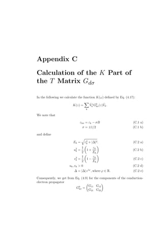
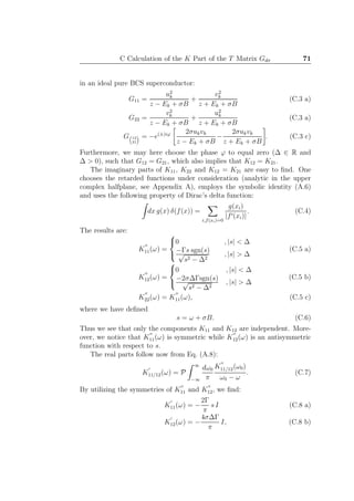
75. C Calculation of the K Part of the T Matrix Gdσ 72
where
I = P
∞
∆
dx fI(x) (C.9)
and
fI(x) =
|x|
√
x2 − ∆2 (x2 − s2)
. (C.10)
We find that the integrand fI(x) displays simple poles at locations x = ±s
and branch points that require a cut line [58] at x = ±∆. Moreover, it is
easy to see that the phase of fI(x) jumps by π when x crosses the cut line.
The integration of I must be done separately for |s| < ∆ and |s| > ∆.
When |s| < ∆, we place the cut line and choose the integration contour in
the complex plane as shown in Fig. C.1. One easily obtains
I(|s| < ∆) =
π
2
√
∆2 − s2
, (C.11)
which yields 


K
′
11(ω) = −
Γs
√
∆2 − s2
K
′
12(ω) = −
2σ∆Γ
√
∆2 − s2
, for |s| < ∆. (C.12)
When |s| > ∆, we use the two slightly different contours depicted in Fig. C.2
and find that I(|s| > ∆) vanishes, which yields:
K
′
11(ω) = K
′
12(ω) = 0 , for |s| > ∆. (C.13)
Two contours are required in order to cancel the integrals infinitesimaly close
to the cut line.
Combining Eqs. (C.5 a), (C.12) and (C.13) we now obtain the result
(4.18) in the main text.

76. C Calculation of the K Part of the T Matrix Gdσ 73
|s|-|s|-D D
x
y
: simple pole
: branch point
: cut line
: integration contour
R
2r e1
e2
infinityR
r
e1
e2
0
0
0
Figure C.1: The integration contour used in the calculation of I (C.9) for |s| < ∆.
|s|-|s| -D D
x
y
(a)
|s|-|s| -D D
x
y
(b)
Figure C.2: The integration contours used in the calculation of I (C.9) for |s| > ∆.
The notation is the same as in Fig. C.1. The Cauchy principal value [58] is taken
at the poles.

77. Bibliography
[1] J. Kondo, Prog. Theor. Phys. 32, 37 (1964).
[2] P. W. Anderson, Phys. Rev. 124, 41 (1961).
[3] J. R. Schrieffer and P. A. Wolff, Phys. Rev. 149, 491 (1966).
[4] M. M. Salomaa, Phys. Rev. B 37, 9312 (1988).
[5] C. A. Stafford and N. S. Wingreen, Phys. Rev. Lett. 76, 1916 (1996).
[6] P. Pals and A. MacKinnon, J. Phys.: Condensed Matter 8, 5401 (1996).
[7] J. Hubbard, Proc. Roy. Soc. A 276, 238 (1963).
[8] A. Theumann, Phys. Rev. 178, 978 (1969).
[9] C. Lacroix, J. Phys. F: Metal Phys. 11, 2389 (1981).
[10] G. Czycholl, Phys. Rev. B 31, 2867 (1985).
[11] A. C. Hewson, Advances in Physics 43, 543 (1994).
[12] T. A. Costi, P. Schmitteckert, J. Kroha, and P. W¨olfle, Phys. Rev. Lett.
73, 1275 (1994).
[13] H. R. Krishna-murthy, Renormalization Group Approach to the Ander-
son Model of Dilute Magnetic Alloys, PhD thesis, Cornell University,
1978.
[14] A. M. Tsvelick and P. B. Wiegmann, J. Phys. C: Condensed Matter 16,
2281 (1983).
[15] R. N. Silver, J. E. Gubernatis, and D. S. Sivia, Phys. Rev. Lett. 65, 496
(1990).
[16] F. B. Anders and N. Grewe, Europhys. Lett. 26, 551 (1994).

78. BIBLIOGRAPHY 75
[17] Henry L. Neal, Jr., Phys. Rev. B 32, 5002 (1985).
[18] Henry L. Neal, Phys. Rev. Lett. 66, 818 (1991).
[19] J. Ferrer, A. Martin-Rodero, and F. Flores, Phys. Rev. B 36, 6149
(1987).
[20] G. Czycholl, A. L. Kuzemsky, and S. Wermbter, Europhys. Lett. 34,
133 (1996).
[21] H. Shiba, Prog. Theor. Phys. 50, 50 (1973).
[22] M. M. Salomaa and R. M. Nieminen, Zeitschrift f¨ur Physik B 35, 15
(1979).
[23] R. Kubo, M. Toda, and N. Hashitsume, Statistical Physics II, Springer-
Verlag, 1985.
[24] D. N. Zubarev, Soviet Physics Uspekhi 3, 320 (1960).
[25] G. Rickayzen, Green’s Functions and Condensed Matter, Academic
Press, 1980, Chapter 2.
[26] G. D. Mahan, Many-Particle Physics, Plenum Press, 1990.
[27] A. Bauer and J. Keller, Zeitschrift f¨ur Physik B 96, 383 (1995).
[28] R. H. Landau, Quantum Mechanics II, Wiley, 1990.
[29] R. D. Harris, J. L. Newton, and G. D. Watkins, Phys. Rev. B 36, 1094
(1987).
[30] J. Hubbard, Proc. Roy. Soc. A 281, 401 (1964).
[31] M. Salomaa, Solid State Communications 23, 291 (1977).
[32] A. T. Alastalo and M. M. Salomaa, Response functions of the anderson
atom, in Proceedings of the XXX Annual Conference of the Finnish
Physical Society, 1996.
[33] K. Yamada, Prog. Theor. Phys. 53, 970 (1975).
[34] M. Salomaa, Zeitschrift f¨ur Physik B 25, 49 (1976).
[35] J. C. Inkson, Many-Body Theory of Solids, Plenum Press, 1984.
[36] H. Schweitzer and G. Czycholl, Zeitschrift f¨ur Physik B , 377 (1990).

79. BIBLIOGRAPHY 76
[37] M. Abramowitz and I. A. Stegun, Handbook of Mathematical Functions,
Dover Publications, Inc., 1965.
[38] M. Salomaa, Solid State Communications 38, 815 (1980).
[39] M. Salomaa, Solid State Communications 39, 1105 (1981).
[40] A. A. Abrikosov, L. P. Gor’kov, and I. Y. Dzyaloshinskii, Quantum Field
Theoretical Methods in Statistical Physics, Pergamon Press, 2 edition,
1965.
[41] A. L. Fetter and J. D. Walecka, Quantum Theory of Many Particle
Systems, McGraw-Hill, 1971.
[42] H. Schweitzer and G. Czycholl, Zeitschrift f¨ur Physik B , 93 (1991).
[43] W. H. Press, S. A. Teukolsky, W. T. Vetterling, and B. P. Flannery,
Numerical Recipes, Cambridge University Press, 2 edition, 1992.
[44] J. N. Lyness and T. J. Kaper, SIAM J. Sci. Stat. Comput 8, 1005 (1987).
[45] M. Blakemore, G. A. Evans, and J. Hyslop, Journal of Computational
Physics 22, 352 (1976).
[46] D. A. Smith and W. F. Ford, SIAM J. Numer. Anal. 16, 223 (1979).
[47] D. Shanks, J. Math. and Phys. 34, 1 (1955).
[48] D. Levin, Intern. J. Computer Math. 3, 371 (1973).
[49] L. R˚ade and B. Westergren, Mathematics Handbook for Science and
Engineering, Studentlitteratur, 3 edition, 1995.
[50] D. Pines and P. Nozi`eres, The Theory of Quantum Liquids, W. A.
Benjamin, 1966.
[51] B. Horvati´c and V. Zlati´c, Phys. Rev. B 30, 6717 (1984).
[52] J. Bardeen, L. N. Cooper, and J. R. Schrieffer, Phys. Rev. 108, 1175
(1957).
[53] M. Tinkham, Introduction to Superconductivity, McGraw-Hill, 2 edition,
1996.
[54] L. P. Gorkov, Sov. Phys. JETP 9, 1364 (1959).
[55] J. J. Sakurai, Modern Quantum Mechanics, Addison-Wesley, 1994.

80. BIBLIOGRAPHY 77
[56] Y. Nambu, Phys. Rev. 117, 648 (1960).
[57] H. Kim and P. Muzikar, Phys. Rev. B 48, 3933 (1993).
[58] G. Arfken, Mathematical Methods for Physicists, Academic Press, 3
edition, 1985.
[59] M. M. Salomaa, private communications, 1996.
[60] O. Gunnarsson and K. Sch¨onhammer, Phys. Rev. B 28, 4315 (1983).
[61] G. R. Stewart, Reviews of Modern Physics 56, 755 (1984).
[62] S. H. Liu, Phys. Rev. B 37, 3542 (1988).
[63] R. Kubo, Rep. Prog. Phys. 29, 255 (1966).