A_Papoulia_thesis2015

The effect of realistic nuclear charge distributions on
atomic levels and transitions
Asimina Papoulia
Master Thesis
Supervisors: Gillis Carlsson & Jörgen Ekman
Division of Mathematical Physics, Lund University
Abstract
Analogue atomic spectral lines from different isotopes display a small shift in energy,
commonly referred as the frequency isotope shift. One of the components of the isotope
shift is the field shift, which depends on the extent and the shape of the nuclear charge
density distribution. In this work, we investigate how sensitive field shifts are with
respect to variations in the nuclear size and shapes. It is found that realistic shapes
of nuclei can have a considerable effect in the prediction of the field shifts. Using a
novel approach, we demonstrate the possibility to extract new information concerning
the nuclear charge densities from the observed field shifts.
1

Contents
1 Introduction 3
2 Theory 3
2.1 Hartree-Fock method . . . . . . . . . . . . . . . . . . . . . . . . . . . . . . . 3
2.1.1 Hartree-Fock approximation . . . . . . . . . . . . . . . . . . . . . . . 4
2.1.2 Variational principle . . . . . . . . . . . . . . . . . . . . . . . . . . . 5
2.1.3 Solving the Hartree-Fock equation . . . . . . . . . . . . . . . . . . . . 6
2.2 Hartree-Fock-Bogoliubov (HFB) method . . . . . . . . . . . . . . . . . . . . 7
2.2.1 BCS approximation . . . . . . . . . . . . . . . . . . . . . . . . . . . . 7
2.2.2 The HFB approximation . . . . . . . . . . . . . . . . . . . . . . . . . 9
2.2.3 Solving the HFB equation for spherical and deformed nuclei . . . . . 9
2.3 Multiconfiguration Dirac Hartree-Fock method . . . . . . . . . . . . . . . . . 10
2.3.1 Solving the relativistic wave equation - Dirac’s equation . . . . . . . . 10
2.3.2 Multiconfiguration approach . . . . . . . . . . . . . . . . . . . . . . . 11
3 Validation of nuclear interaction 12
3.1 Background . . . . . . . . . . . . . . . . . . . . . . . . . . . . . . . . . . . . 13
3.2 Method . . . . . . . . . . . . . . . . . . . . . . . . . . . . . . . . . . . . . . 14
3.2.1 Folding of proton density . . . . . . . . . . . . . . . . . . . . . . . . 14
3.2.2 Comparison of the theoretical models . . . . . . . . . . . . . . . . . . 16
3.3 Accuracy of theoretical models . . . . . . . . . . . . . . . . . . . . . . . . . . 18
3.3.1 The realistic HFB models . . . . . . . . . . . . . . . . . . . . . . . . 18
3.3.2 The Fermi model . . . . . . . . . . . . . . . . . . . . . . . . . . . . . 20
3.3.3 The effect of folding . . . . . . . . . . . . . . . . . . . . . . . . . . . 21
4 Atomic isotope shift 22
4.1 Mass shift . . . . . . . . . . . . . . . . . . . . . . . . . . . . . . . . . . . . . 22
4.2 Field shift . . . . . . . . . . . . . . . . . . . . . . . . . . . . . . . . . . . . . 23
4.2.1 Variational approach . . . . . . . . . . . . . . . . . . . . . . . . . . . 23
4.2.2 Perturbative methods . . . . . . . . . . . . . . . . . . . . . . . . . . . 24
4.2.3 Validation of perturbative method . . . . . . . . . . . . . . . . . . . . 25
5 The effect of realistic nuclear charge distributions 27
5.1 Higher order moments in field shift . . . . . . . . . . . . . . . . . . . . . . . 28
5.1.1 Spherical nuclei . . . . . . . . . . . . . . . . . . . . . . . . . . . . . . 28
5.1.2 Deformed nuclei . . . . . . . . . . . . . . . . . . . . . . . . . . . . . . 30
5.2 Experimental isotope shifts . . . . . . . . . . . . . . . . . . . . . . . . . . . . 33
5.3 Extracting higher moments from data . . . . . . . . . . . . . . . . . . . . . . 35
5.3.1 RFS expansion in orthonormal basis . . . . . . . . . . . . . . . . . . 36
5.3.2 Extraction of δ r2
and δ r4
. . . . . . . . . . . . . . . . . . . . . . 37
5.3.3 Uncertainties in the extraction of δ r2
and δ r4
. . . . . . . . . . . 41
6 Results 43
7 Outlook 45
2

1 Introduction
The abundance of an isotope for a particular element varies between different astronomical
objects and on a long-term scale it also varies from time to time depending on its decay rate.
Therefore, the knowledge of the origin and evolution process of the astronomical objects
existing in the Milky Way and other Galaxies depends not only on their elemental but
also on their isotopic composition. Although the chemical composition of the Earth is well
known, the study of the isotopes abundance in various stars and other planets is still of great
interest. In addition, such studies are not restricted to the natural elements. They can also
be expanded into the investigation of radioactive isotope abundances, artificially produced
in laboratories.
Light coming from astronomical objects can be analyzed through the resulting spectra.
Most commonly the energy spectra consist of several lines of different wave-lengths and
intensities. For a particular element, the spectra of the various isotopes are very similar.
A small shift in wave-length is however observed, known as the frequency isotope shift. As
a result, the intensity of such peaks represents the isotopes abundance. By measuring the
difference in frequency between two peaks representing analogue transitions, we can calculate
the corresponding difference between the nuclear radii of the isotopes represented by these
peaks. Thus, by using one isotope as reference we can identify the existing variety of isotopes.
For light nuclei, the difference in frequency is dominated by the difference in the second
order radial moment δ r2
, since the contribution of higher order radial moments of the
nuclear charge density distribution on the frequency shift is almost negligible. However,
in heavier systems the higher moments contribute to a particular percentage to this shift.
Therefore, further conclusions can be drawn on the deformation, density wiggles etc. of
the nuclear charge distributions in such systems. The main objective of this thesis is to
study the effect of the higher order radial moments from realistic charge distributions on the
frequency isotope shift in these heavy nuclear systems. We restrict ourselves to highly ionized
lithium-like atomic systems, since for such systems the calculations become simplified.
Chapter 2 provides the theoretical background needed in order to calculate the nuclear
densities, as well as the atomic levels and transition energies. Next, chapter 3 illustrates
the validity of the nuclear interaction by performing a systematic study of the higher order
radial moments of the nuclear charge density distributions. A reformulation of the field shift
component of the isotope shift is introduced, in chapter 4, for the heavy nuclear systems. The
reformulated field shift is, in chapter 5, used in order to estimate the effect that the realistic
nuclear distributions have on the atomic levels and transitions. At last, it is explained how
the observed isotope shifts can be used in order to extract the nuclear radial moments and
therefore draw conclusions on the nuclear size and shape of the isotopes.
2 Theory
2.1 Hartree-Fock method
In microscopic systems the treatment of many-body problems is not a trivial task, even
if the number of particles is not large. It is well known that in the simplest one-particle
case of a Hydrogen atom, the Schrödinger equation can have an exact solution from which
the eigenfunctions and eigenvalues of the system are obtained. However, for a N particle
3

system the Schrödinger equation is impossible to solve exactly. Therefore, methods have been
developed to make it possible to obtain an approximate solution for such systems, by reducing
the case to a one-particle problem. These approximations are called mean-field methods.
In particular, Hartree-Fock (HF) is a mean-field method widely used for the description
of many-body systems, constituting a principal tool for the description of both nuclear and
atomic states. Furthermore, the HF method constitutes the starting point for the formulation
of more sophisticated methods, like BCS and Hartree-Fock-Bogoliubov (HFB), which will be
discussed in the upcoming section 2.2.
2.1.1 Hartree-Fock approximation
The main idea of the Hartree-Fock method is based on the assumption that the potential be-
tween the numerous particles of a system can be approximated by an averaged single-particle
(mean-field) potential, so that the Hamiltonian of this many-body system is reduced to a
single-particle Hamiltonian. This procedure is known as the Hartree approximation. Initially
the Hamiltonian has the following form:
ˆH = ˆT + ˆV = −
1
2m
n
i=1
∇2
i +
1
2
n
i=j
u(ri, rj),
where the first term is the sum of the kinetic energy of all individual particles and the
second term represents the potential energy between two particles, summed up for all possible
combinations. The factor of 1
2
ensures that terms like u(r1, r2) and u(r2, r1) are taken into
account only once. The i = j restriction on the sum ensures that particles do not interact
with themselves. After the approximation the Hamiltonian above reduces to a one-particle
Hamiltonian:
ˆHHartree = −
1
2m
∇2
+ VH(r).
However, this method does not take into account the fermionic nature of particles. To
achieve this, the Hartree-Fock approximation makes the assumption that the total wave
functions of the interacting particles could take the form of a Slater determinant, so that
they obey the antisymmetry property. The linear eigenvalue problem then has the form:
ˆHHF |ψ = EHF
|ψ ,
with an additional Fock term VF included now in the potential of the total Hartree-Fock
Hamiltonian. For n-particles occupying n different orbitals {φi}i=1...n the wave function ψ
is a linear combination of products of these orbitals φi, with their coordinates {−→ri }i=1...n
permuted in all possible ways with a change of sign when the number of two-coordinate
permutations (p) is odd [3]:
ψ(−→r1 , −→r2 , ..., −→rn) =
P
(−1)p
√
n!
P[φ1(−→r1 )φ2(−→r2 )...φn(−→rn)].
The sum over P means the sum over all possible permutations of the particles coordinates
and p is the number of two-coordinate permutations required to obtain the product of orbitals
in its initial form, i.e. φ1(−→r1 )φ2(−→r2 )...φn(−→rn). Therefore, the ansatz we make has the form
4

of a Slater determinant, which (normalized for a combination of n particles) can also be
equivalently written:
ψ(−→r1 , −→r2 , ..., −→rn) =
1
√
n!
φ1(−→r1 ) φ2(−→r1 ) . . . φn(−→r1 )
φ1(−→r2 ) φ2(−→r2 ) . . . φn(−→r2 )
...
...
...
...
φ1(−→rn) φ2(−→rn) . . . φn(−→rn)
.
For a given complete set of orthonormal orbitals {φi}i=1...n we can construct a complete
set of all possible Slater determinants, which are also orthonormal. This complete set of
orthonormal Slater determinants is said to form the Fock space [3].
2.1.2 Variational principle
To obtain the most appropriate wave function, we must choose among all possible Slater
determinants ψ the one that yields the lowest total energy. According to the variational
principle:
EHF
g.s. ≤
ψ | ˆH | ψ
ψ | ψ
,
the ground state (g.s.) energy will always be the lowest bound of a variational calculation.
For a trial wave function then the ground state energy is always larger than or ideally equal
to the exact ground state energy:
EHF
g.s. = ψ ˆHHF ψ ≥ Etrue
g.s.
Therefore, the closer the trial wave function is to the exact ground state wave function the
more representative it will be for the given system of interacting particles. The expectation
value of the Hartree-Fock Hamiltonian will be calculated by using the occupation number
representation [23]. We will then minimize the total ground state energy with respect to
all possible choices of the n existing orbitals {φi}i=1...n by applying the method of Lagrange
multipliers.
Thus, we vary the total energy with respect to an inﬁnitesimal change in the orbitals
φi(−→r ), e.g. δE =limε→0
E[φi+εδφi]−E[φi]
ε
. Requiring that the energy is stationary with
respect to variations and putting as constraint the fact that the orbitals must be normalized,
we get:
δE = δ ψ ˆH ψ −
i
ǫi d−→r |φi|2
= 0,
which yields the Hartree-Fock equation [4]:
ˆT + VH + ˆVF φk(−→r ) = ǫkφk(−→r ),
where
VH(r1) = u(r1, r2)ρ(r2)dr2,
5

is the Hartree potential that depends on the local particle density ρ(r2) and expresses the
potential energy of a particle at point r1 due to the interaction u(r1, r2) and ˆVF is the Fock
operator based on the Fock potential:
VF (r1, r2) = −u(r1, r2)ρ(r1, r2),
which depends on the non-local density ρ(r1, r2). Hence, the Hartree term can be written as
a potential which is common for all particles, while the Fock term gives in fact rise to slightly
different potentials for each particle.
2.1.3 Solving the Hartree-Fock equation
Since both the Hartree and Fock potentials depend on the orbitals φi(−→r ), the HF equation
derived above is non-linear. Therefore, this equation can only be solved self-consistently
using the method of iterations by following the steps that are described below:
1. We start by making an initial guess for the orbitals {φi}i=1...n .
2. Particle density ρold(−→r ) and particle non-local density ρold(−→r , −→r ′
) can be calculated.
3. From the densities found in step 2 (or 6), we can calculate the potentials: VH[ρ(r)] and
VF [ρ(−→r , −→r ′
)]respectively and build the total Hamiltonian of the system.
4. Keeping VH and VF fixed, we can now solve the Hartree-Fock equation:
ˆT + VH + ˆVF φk(−→r ) = ǫkφk(−→r ),
which yields new orbitals φk(−→r ).
5. Subsequently, the new orbitals yield new densities ρnew(−→r ) and ρnew(−→r , −→r ′
) respec-
tively.
6. The new densities are used now, after some mixing with the old ones - the reason of
this mixing will be explained soon - , as a new input so that we can start again from
step 3.
We repeat the described process until convergence is reached. In other words, we continue
until the difference between the new and old density is smaller than some chosen tolerance.
The most common trick used in order to achieve convergence is to mix the densities from
the previous iteration with the new densities obtained from step 5 above. An extra step
is then added to the method. Hence, after step 4 we define (for each iteration m that is
performed) the new mixed densities as ρnew = αρ(m)
+ (1 − α)ρ(m−1)
, where α is a parameter
that determines the amount of mixing.
In order to solve the HF equation in step 4, we work in a configuration space based on
some arbitrary complete and orthogonal set of single-particle wave functions. The most
commonly used set is the harmonic oscillator (HO) wave functions. Thus, each one of
the orbitals {φi}i=1...n is written as linear combination of these HO wave functions, e.g.
6

φ1(−→r1 ) =
N
i=1
c1
i bi(−→r1 ) where N is the number of basis functions that are used for the expan-
sion. The coefficients cj
i are then determined in such a way that the corresponding energy
has a minimum (variational principle). The HF equation is eventually transformed into a
matrix eigenvalue equation that can be solved using existing numerical methods.
2.2 Hartree-Fock-Bogoliubov (HFB) method
The procedure of solving the HF equation self-consistently for a system of particles inside a
nucleus provides us with a rather satisfactory description of the nuclear charge density distri-
bution. However, in order to be able to understand and describe phenomena experimentally
observed, like the spectral energy gap in even-even nuclei, we have to take into account the
correlations due to the short-range part of the nucleon-nucleon interaction, called pairing [16].
Thus, by enhancing the HF method we will be capable of laying out an improved description
of the nuclear charge density distributions and their properties, i.e. rms (root-mean-square)
radii and higher order radial moments.
Pairing correlations are described in the BCS method, developed by the solid-state physi-
cists Bardeen, Cooper and Schrieffer (BCS) in 1957, so that it could be applied to the theory
of superconductivity. Later, the same theory was also applied to nuclei by Bohr, Mottelson
and Pines in 1958 [13] after they realized that the effect of pair interaction was analogous
to the superconductivity in metals. Therefore, using the wave-function suggested by BCS,
whose form is demonstrated below, as ansatz (instead of the more simplified Slater determi-
nant) and vary the new wave function to find again the minimum of the energy after having
already solved HF equations leads to a more powerful approximation for the description of
nuclear many-body systems. Finally, the BCS approximation in turn, constitutes the starting
point of the formulation of the Hartree-Fock-Bogoliubov (HFB) method.
2.2.1 BCS approximation
The concept of pairing correlations implies that the motion of nucleons is disturbed by
their interactions with other nucleons. Thus, nucleons can be seen as quasi-particles (same
undisturbed particles but with different masses). Hence, in the BCS approximation the
quasi-particle formalism is used. We look for a more general product of wave functions
consisting of independently moving quasi-particles and thus, we make an ansatz different
from the Slater determinant that is used in the HF method. The most appropriate ansatz
has been proven to be the one analogous to the ground state wave function suggested by
Bardeen, Cooper and Schrieffer for determining the ground state of a superconductor. The
BCS wave function for nuclei is then illustrated in the following way:
ψBCS
o =
ν
(Uν + Vνα+
ν α+
ν ) |0 ,
where |0 is the vacuum state and V ν, Uν represent variational parameters. These parameters
are subject to the constraint V 2
ν+U2
ν = 1 due to the normalization condition, since they are
regarded as the probability that a certain HF pair state (ν, ν) is or is not occupied respectively.
Additionally, according to the variational principle these parameters are determined in such
a way that the corresponding energy has a minimum.
7

In the HF method, a Slater determinant type wave-function is used as ansatz. Given the
fact that it represents particles that occupy the orbitals independently, this ansatz is not able
to reproduce the desirable results. On the other hand, the BCS wave function provides a
more accurate description of the system as it always contains a term with the right number
of particles that occupy orbitals in pairs. However, the new ansatz contains also terms with
the wrong number of particles. This is well illustrated by considering the simplest case of
two existing levels and comparing them to the corresponding two-particle Slater determinant.
We consider then a space with two two-fold degenerate levels, called s and r. The solution
with the lowest energy is frequently obtained when the particles occupy the lowest levels.
Therefore, according to the definition of the Slater determinant in 2.1.1, the wave function
for two particles occupying these levels will be given by:
ψ(1, 2) =
1
√
2
(φs(r1)φs(r2) − φs(r2)φs(r1))
or
ψ = α+
s α+
s |0 ,
which in fact represents the independent orbital occupation of two particles s and s in the
lowest orbital. Thus, the wave-function consists of only one Slater determinant. On the other
hand, the BCS wave function represents particles in pairs occupying the orbitals. Hence, for
two pairs of particles occupying same, as before, levels s and r, the wave-function takes the
form:
ψBCS
= (Ur + Vrα+
r α+
r )(Us + Vsα+
s α+
s ) |0 ,
which can be written:
ψBCS
= (ψ(0) + ψ(2) + ψ(4)),
where
ψ(0) = UrUs |0 ,
ψ(2) = (VrUsα+
r α+
r + UrVsα+
s α+
s ) |0 ,
ψ(4) = VrVsα+
r α+
r α+
s α+
s |0 .
We then deduce that the first component contains no pairs, the second component contains
one pair, which alternatively occupies levels s and r, and the third component describes
a situation where both levels are occupied by these two pairs. Therefore, only one of the
terms, that is ψ(2), contains the proper quantity of particles. In this case, we need to find
the right way to treat the total wave function so that we take as average the right amount
of particles. In fact, each component in the expression of the wave function contributes to
a particular extent to the description of a system’s state. The resulting weighted terms will
then reproduce the right number of particles by making use of an additional constraint during
the minimization process of the Hamiltonian, using BCS as wave-function.
According to the variational principal we minimize the total ground state energy with
respect to all possible choices of the U and V coefficients. However, we minimize the energy
by calculating the expectation value of ˆH′
= ˆH − λ ˆN, that is
EBCS
=
ψBCS ˆH′ ψBCS
ψBCS | ψBCS
=
ψBCS ˆH − λ ˆN ψBCS
ψBCS | ψBCS
,
8

where λ is a Lagrange multiplier and ˆN the number operator defined as:
ˆN =
ν
α+
ν αν + α+
ν αν ,
summing over all the pair states (ν, ν). Therefore, the condition that assures that the
average number of particles equals the actual number of particles, N, is represented by
N = ψBCS ˆN ψBCS
= N . Combined with the normalization condition, parameters Vν
and Uν can now be fully determined.
2.2.2 The HFB approximation
According to the previous subsection 2.2.1, the BCS wave function is used in order to provide
a more appropriate representation of nuclear states. Therefore, based on the mean-field that
was already found in the HF method we perform again the minimization process of the
energy in order to determine parameters Vν and Uν for each HF pair state (ν, ν). The
Hartree-Fock-Bogoliubov (HFB) method is similar to the BCS method. However, in HFB,
during the minimization of the Hamiltonian we minimize with respect to both the Vν and Uν
coefficients, as well as the orbitals. In this case, the mean-field is also varied.
2.2.3 Solving the HFB equation for spherical and deformed nuclei
The iterative process is also used in the new approximation, and HFB equations are solved
using the simple iterative diagonalization method with mixing of orbitals as described in
1.1.3. Hence, same mixing tricks are used in order to facilitate convergence. Moreover, the
harmonic oscillator (HO) basis is again used in the HFB method for expanding the single-
particle wave-functions of neutrons and protons for a given nuclear state. For A particles
and considering the HF-limit, the particle density is written:
ρ(−→r ) =
A
i
|φi(−→r )|
2
=
A
i=1
φ∗
nilijimi
(−→r )φnilijimi
(−→r ),
which is the sum of all individual particle densities for all A particles, with each one of
them being in a particular nljm state. Each one of the occupied orbitals {φi}i=1...A is a
linear combination of the HO wave functions. Using jj-coupling, the particle density can be
written as:
ρ(−→r ) =
JM
ρJM (r)YJM (θ, ϕ),
meaning that the particle density can finally be written as a superposition of all possible JM
quantum states.
For the case of a spherical shell model the sum of the HO wave functions, used as a basis
for the calculations, must be spherical. Therefore, we restrict ourselves to spherical symmetry
by taking into consideration only the part for which J = MJ = 0. In spherical symmetry,
the solutions to the HFB equations are provided by HOSPHE (v2.00) which is a new version
of the program HOSPHE (v1.02) [7]. On the contrary, in the study of deformed nuclei, l, j
and mj are no longer “good” quantum numbers and consequently spherical symmetry breaks
down. Therefore, it is essential to take into account more quantum states for a variety of J
9

and MJ values, so that the particle density will be a superposition of several JM quantum
states. In the case of deformed nuclei, the HFB equations are solved by HFBTHO (2.00d)
[22], using the cylindrically deformed HO basis.
2.3 Multiconfiguration Dirac Hartree-Fock method
The Multi-Configuration Dirac-Hartree-Fock (MCDHF) approach is used for the determina-
tion of atomic properties. In contrast to nuclear systems where the non-relativistic Schrödinger
equation is solved, in atoms it is necessary to make use of a relativistically correct expression
for the kinetic energy. The electrons move with relativistic velocities around the nucleus
and thus, the relativistic effects play an important role in the determination of their bound
states. Hence, the Dirac’s equation is solved instead. Furthermore, the wave-functions are
now configuration state functions that are formed by angular coupling of the orbitals in an
electron configuration. The calculations based on the MCDHF approach are performed with
the new version of the GRASP2K relativistic atomic structure package [11].
2.3.1 Solving the relativistic wave equation - Dirac’s equation
In nuclear systems, the non-relativistic expression for the Hamiltonian is given by:
ˆH =
ˆp2
2m
+ ˆV ,
and the eigenvalue problem is of the form:
ˆHψ(r) = (
ˆp2
2m
+ ˆV )ψ(r) = Eψ(r),
which is the time-independent Schrödinger’s equation, where ψ(r) are the wave-functions
describing the system. However, in atomic systems, for the kinetic energy of the electrons
we need to use the relativistic expression:
(E − V ) = (pc)2 + (m0c2)2,
for particles moving under the influence of a potential V . Here, m0 is the electron’s rest
mass. Hence, one may postulate:
(H − V )2
ψ = (−i c∇)2
ψ + (m0c2
)2
ψ.
According to Dirac, Schrödinger’s equation for spin-1
2
particles can take the form:
HΨ = −( c)2∇2 + (m0c2)2Ψ + V Ψ,
where Ψ is a column matrix or spinor:
Ψ(r) =




ψ1(r)
ψ2(r)
ψ3(r)
ψ4(r)



 ,
10

with the wave-functions ψ representing respectively spin-up and spin-down states of a particle,
as well as spin-up and spin-down states of the corresponding antiparticle. It can then be
shown that the Dirac-Coulomb Hamiltonian can be written as:
HDC




ψ1
ψ2
ψ3
ψ4



 = c(αp + βm0c)




ψ1
ψ2
ψ3
ψ4



 + VC




ψ1
ψ2
ψ3
ψ4



 ,
where αp =




0 0 pz px − ipy
0 0 px + ipy −pz
pz px − ipy 0 0
px + ipy −pz 0 0



 and β =




1 0 0 0
0 1 0 0
0 0 −1 0
0 0 0 −1



. The
eigenvalue problem then takes the form:
(E − VC)




ψ1
ψ2
ψ3
ψ4



 = c




m0c 0 pz px − ipy
0 m0c px + ipy −pz
pz px − ipy −m0c 0
px + ipy −pz 0 −m0c








ψ1
ψ2
ψ3
ψ4




This is a set of four simultaneous, partial differential equations that needs to be solved in
order to obtain all the components of the energy eigenfunctions ψ(r). However, two of these
eigenfunctions correspond to antiparticle states that are states of negative energy and they
are of less significance in our calculations. Since no transition between positive and negative
energy states occurs, the negative energy states can be neglected.
2.3.2 Multiconfiguration approach
In the previous section, we discussed Dirac’s equation that solves the relativistic wave func-
tion, establishing spin s as an additional degree of freedom for elementary particles, like
electrons. Hence, the spin of the electrons will now be coupled to their orbital angular
momentum l, so that their total angular momentum is given by j = l + s.
In n-electron systems, the Dirac-Coulomb Hamiltonian is given by:
ˆHDC =
n
i=1
[c(αp + βm0c) + V N
i ] +
1
2
n
i=j
1
|ri − rj|
,
where the Coulomb potential between two electrons:
n
i=j
1
|ri−rj|
corresponds to the potential
produced due to the two-particle interaction, generally expressed as 1
2
n
i=j
u(ri, rj) in 2.1.1. In
the expression above V N
i is the electron-nucleus Coulomb interaction, which in the case of a
point-like nucleus reduces to V N
i = −Z
ri
. However, assuming an extended charge distribution
V N
i may be slightly different for two isotopes which ultimately causes the field shift between
analogue transitions in an isotope pair. According to the mean-field approximation, the
Hamiltonian of the many-electron system then reduces to the Dirac-Hartree-Fock (DHF)
Hamiltonian:
11

ˆHDHF = c(αp + βm0c) + V N
i + VH + ˆVF ,
Due to the spherically symmetric charge distribution of the electrons, it is radially symmetric.
Therefore, only the radial part of the Hamiltonian is the one that must be calculated through
a self-consistent field procedure similar to the one described in 2.1.3.
In order to estimate the potential VH + ˆVF , we have to find approximate electron wave
functions for the atomic states. A single Slater determinant (see 2.1.1) is not necessarily an
eigenfunction of the atomic system and therefore linear combinations of determinants are
used instead. These linear combinations are called configuration state functions (CSFs) and
they are denoted as Φ(γPJMJ ), where γ represents the electron configuration. The notation
indicates that the CSFs are state functions with the same parity P, total angular momentum
J and component MJ along the z-direction. Finally, the atomic state functions (ASFs) Ψ
will be a so-called multiconfiguration expansion over the CSFs, so that we can write:
Ψ(γPJMJ ) =
N
i=1
ciΦ(γiPJMJ ),
where ci are referred to as mixing coefficients with
N
i=1
c2
i = 1. The most appropriate wave
function Ψ, which describes a state of the given system, is obtained through an optimization
process by applying the variational principle (see 2.1.2). The expression for the approximate
state energy will now be:
E(γPJMJ ) =
N
i=1
N
j=1
cicj Φ(γiPJMJ ) ˆH Φ(γjPJMJ ) .
The mixing coefficients then need to be determined, based on the argument that the energy is
stationary with respect to variations. This process finally yields a set of coupled differential
equations that are similar to the HF equations, which need again to be solved iteratively
until convergence is reached (see 2.1.3).
3 Validation of nuclear interaction
The main purpose of this section is to demonstrate the validity of the nuclear interaction
based on the selected Skyrme-type forces and to investigate which set of parameters is the
most appropriate. For that reason, the nuclear charge density distributions are calculated for
a variety of isotopes and compared to the experimental data, already obtained in 1987, from
elastic electron scattering experiments [25]. Having obtained the best possible description of
the charge density distributions, it is then feasible to determine fundamental properties of
the atomic nucleus, like the rms charge radii, which, together with higher radial moments
values, give a satisfactory measurement of its size and shape.
The determination of nuclear properties constitutes a fundamental part of nuclear physics,
but it seems to effect at a particular extent atomic physics, too. Phenomena observed, like
the small shift in atomic energy levels and transitions among different isotopes, are due to
12

the differences in mass and size, as well as the shape differences of the nuclear charge density
distributions. Therefore, it is of great importance to achieve the best possible description of
the nuclear systems in order to predict the effect on isotope field shifts in atoms (see Chapter
4). For comparison, higher order radial moments are also calculated for a two-parameter
Fermi distribution. Thus, we can compare the radial moments resulting from the more
realistic HFB distributions with the ones resulting from the simplified Fermi distribution.
The actual purpose of this procedure is to be able to finally compare the effect that these two,
slightly different, distributions have on the field shifts that are being investigated throughout
the next two chapters.
3.1 Background
The forces acting between the nucleons give rise to an average single-particle potential ac-
cording to the mean-field methods. The form of the potential term of the Hamiltonian, then
depends on the choice of the interaction. Since it is impossible to microscopically calculate
the interactions between nucleons, especially for the case of heavy nuclei, the only way is
to use phenomenological forces that contain a certain number of parameters. By adjusting
these parameters, we try to reproduce as many experimental data as we can. The Skyrme
interaction is a phenomenological effective nucleon-nucleon interaction that is applicable to
many-body methods and seems to be the fastest one when we solve HF or HFB equations
by using numerical methods.
In order to formulate the effective nucleon-nucleon interactions, we require the trans-
lational and rotational symmetries, exchange of coordinate invariance etc. to be fulfilled
[17]. Moreover, the four possible ways -depending on the spin component- that protons and
neutrons interact with each other, as well as the spin-orbit interaction, must be taken into
consideration in the expression for the potential. Lastly, even if the two-body forces are the
strongest inside the nucleus, a three-body term is included and provides an enhanced de-
scription of the nuclear model. Therefore, the Skyrme interaction potential contains a two-
and a three-body term, as it is shown below:
V = i<j V (i, j) + i<j<k V (i, j, k),
where the two- and three-body terms are respectively:
V (1, 2) = t0(1 + x0Pσ
)δ(−→r1 − −→r2 )+
+
1
2
t1[δ(−→r1 − −→r2 )
−→
k2
+ k2δ(−→r1 − −→r2 )] + t2kδ(−→r1 − −→r2 )k+
+iW0(σ(1)
+ σ(2)
)k × δ(−→r1 − −→r2 )k,
where k = 1
2i
(∇1 − ∇2) is the operator of the relative momentum, and:
V (1, 2, 3) = t3δ(−→r1 − −→r2 )δ(−→r2 − −→r3 )
The short range expansion of the two-body term (that is used to simplify the calculations) and
the zero-range force that has been assumed for the three-body term contain a certain number
of parameters, i.e. t0, t1, t2, t3, x0 and W0, adjusted to reproduce the experimental data that
has been adopted. In many Skyrme parametrizations the original three-body force is often
13

replaced by a density-dependent two-body interaction which makes the method similar to
density functional theory. In addition, the mathematical form of this force is extremely
simple, as it includes δ-functions that can simplify the calculations to a great extent, and as
a consequence make them fast enough [18].
3.2 Method
Two different sets of parameters have been selected for the theoretical calculations of the
nuclear charge density distributions. These are called SLY4 and UDF1. In order to check
the range of validity of these two parametrizations of Skyrme interactions, we made a com-
parison of theoretical and experimental charge distributions. This comparison concerns the
proton densities of the selected nuclei, since these are the only ones that can be measured
experimentally.
3.2.1 Folding of proton density
The initial calculations were carried out assuming that protons are point particles. Hence, an
initial representation of proton densities inside various nuclei was obtained. However, protons
are composite particles, made of quarks. In order to achieve a more accurate description of the
charge density distributions, we “folded” the proton densities using the convolution formula:
̺c(r) = d3
r′ρp(r′)g( r − r′ ),
where ρp(r) is the initially calculated proton density and
g(r) = (r0
√
π)−3
e−(r/r0)2
,
the form factor, which is assumed a Gaussian with r0 = 2
3
rp rms [6]. Since the proton ra-
dius determination experiments have resulted in different values, it is essential to use a proton
radius value that is more realistic. Experiments based on electron scattering measurements
have displayed proton radius rp rms = 0.88 fm [19]. On the other hand, in experiments where
muonic hydrogen was used the radius was found to be rp rms = 0.84 fm [15]. Of course,
a physical parameter can not depend on the method of extraction. Hence, until the proton
radius puzzle is finally solved we performed the calculations by assuming rp rms = 0.88 fm.
However, later in the results the case of folding for a different proton radius value is com-
pared, so that we can draw further conclusions of the effect of the proton size in the folding
process.
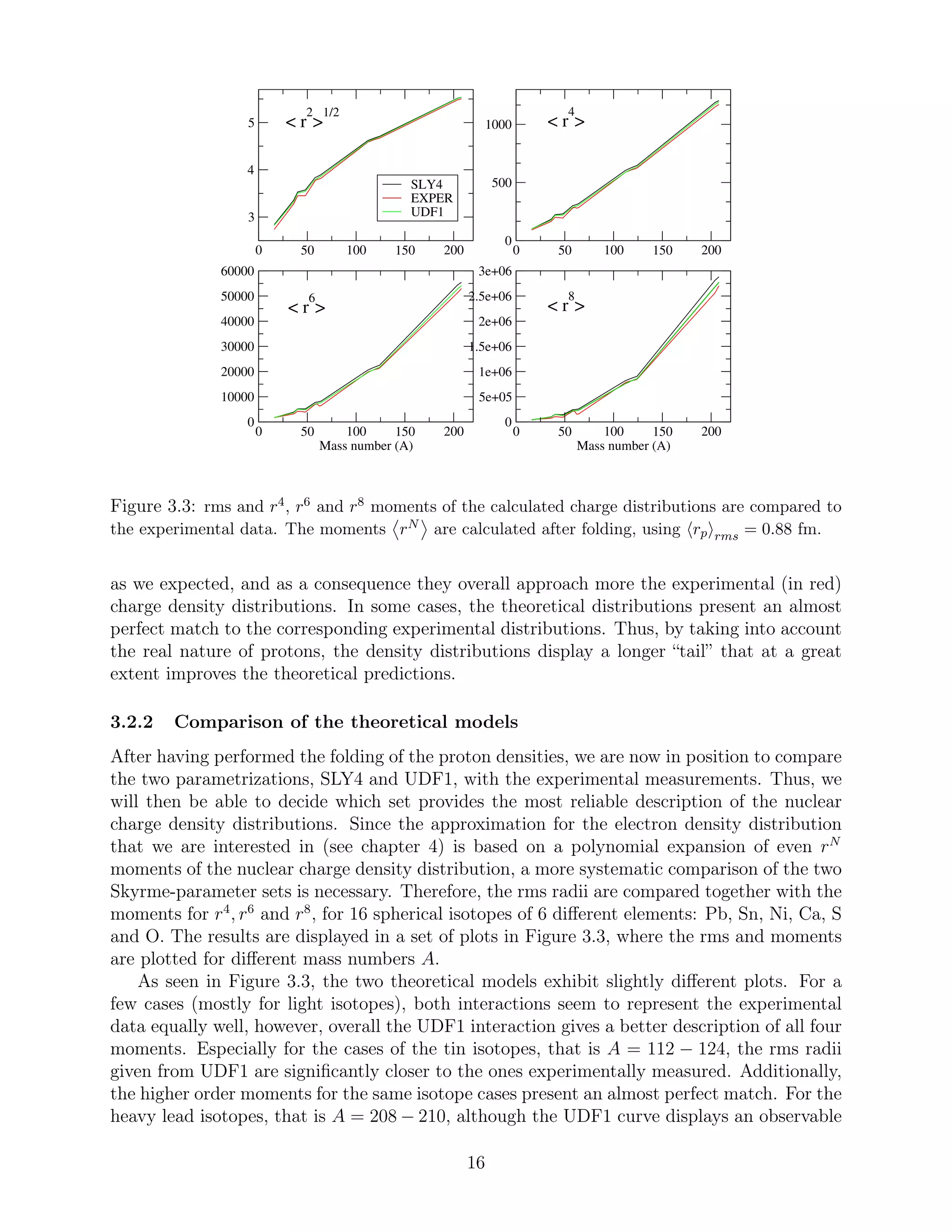
The effect of folding, for each one of the sets of parameters, is separately shown in Figure
3.1 for the SLY4 parameter set and in Figure 3.2 for the UDF1 parameter set. The “old”
proton densities and the “folded” nuclear charge density distributions are compared with the
corresponding experimental charge density for some chosen elements. In order to make the
comparison with the experimental curve easier and at the same time highlight the effect of
convolution to the proton densities, we plotted the logarithm of the proton density values
against the radius r measured in fermi (fm).
Considering the four different nuclei illustrated, we deduce that the “folded” proton den-
sities (in black for SLY4 and green for UDF1), for both sets of parameters, are smeared out
14

0 5 10
0.0001
0.001
0.01
log(protondens)
Folded
Exper.
Old
0 5 10
0.0001
0.001
0.01
0 5 10
r [fm]
0.0001
0.001
0.01
log(protondens)
0 5 10
r [fm]
0.0001
0.001
0.01
60
Ni
40
Ca
208
Pb 112
Sn
Figure 3.1: Comparison of experimental data with theoretically calculated nuclear charge density
distributions for several isotopes using the SLY4 set of parameters. The curve labeled “Old” corre-
sponds to the charge density assuming point-like protons. For the curve labeled “Folded” the quark
structure of the protons is taken into account by a folding method using rp rms = 0.88 fm.
0 5 10
0.0001
0.001
0.01
log(protondens)
Folded
Exper.
Old
0 5 10
0.0001
0.001
0.01
0 5 10
r [fm]
0.0001
0.001
0.01
log(protondens)
0 5 10
r [fm]
0.0001
0.001
0.01
208
Pb
112
Sn
60
Ni
40
Ca
Figure 3.2: Same as Figure 3.1 but for the UDF1 set of parameters.
15

0 50 100 150 200
3
4
5
SLY4
EXPER
UDF1
0 50 100 150 200
0
500
1000
0 50 100 150 200
Mass number (A)
0
10000
20000
30000
40000
50000
60000
0 50 100 150 200
Mass number (A)
0
5e+05
1e+06
1.5e+06
2e+06
2.5e+06
3e+06
< r
4
>
< r
8
>< r
6
>
< r
2
>
1/2
Figure 3.3: rms and r4, r6 and r8 moments of the calculated charge distributions are compared to
the experimental data. The moments rN are calculated after folding, using rp rms = 0.88 fm.
as we expected, and as a consequence they overall approach more the experimental (in red)
charge density distributions. In some cases, the theoretical distributions present an almost
perfect match to the corresponding experimental distributions. Thus, by taking into account
the real nature of protons, the density distributions display a longer “tail” that at a great
extent improves the theoretical predictions.
3.2.2 Comparison of the theoretical models
After having performed the folding of the proton densities, we are now in position to compare
the two parametrizations, SLY4 and UDF1, with the experimental measurements. Thus, we
will then be able to decide which set provides the most reliable description of the nuclear
charge density distributions. Since the approximation for the electron density distribution
that we are interested in (see chapter 4) is based on a polynomial expansion of even rN
moments of the nuclear charge density distribution, a more systematic comparison of the two
Skyrme-parameter sets is necessary. Therefore, the rms radii are compared together with the
moments for r4
, r6
and r8
, for 16 spherical isotopes of 6 different elements: Pb, Sn, Ni, Ca, S
and O. The results are displayed in a set of plots in Figure 3.3, where the rms and moments
are plotted for different mass numbers A.
As seen in Figure 3.3, the two theoretical models exhibit slightly different plots. For a
few cases (mostly for light isotopes), both interactions seem to represent the experimental
data equally well, however, overall the UDF1 interaction gives a better description of all four
moments. Especially for the cases of the tin isotopes, that is A = 112 − 124, the rms radii
given from UDF1 are significantly closer to the ones experimentally measured. Additionally,
the higher order moments for the same isotope cases present an almost perfect match. For the
heavy lead isotopes, that is A = 208 − 210, although the UDF1 curve displays an observable
16

0 50 100 150 200
3
4
5
SLY4
EXPER
UDF1
0 50 100 150 200
0
500
1000
0 50 100 150 200
Mass number (A)
0
10000
20000
30000
40000
50000
60000
0 50 100 150 200
Mass number (A)
0
5e+05
1e+06
1.5e+06
2e+06
2.5e+06
3e+06
< r
6
> < r
8
>
< r
4
>< r
2
>
1/2
Figure 3.4: rms and r4, r6 and r8 moments, calculated based on the Fermi distribution model, are
compared to the experimental data.
difference from the experimental one, it keeps representing better the values than the curve
resulting from the SLY4 model. Lastly, observing all four plots at the same time we can
deduce that the higher the order of the calculated moment is, the more the UDF1 interaction
becomes appropriate.
In calculations of electron states in atoms, the nucleus is often approximated as a Fermi
distribution. In this way, one may take into account that the nucleus is not a point-like
particle and obtain a more realistic potential for the electrons. In such a model, the Fermi
distribution approximating the nuclear charge distribution takes the form:
ρ(r) =
ρ0
1 + e
(r−c)
α
,
which is a spherical two-parameter model. The parameter α is given by the relation:
t = 4 ln(3)α,
where t is the skin thickness of the distribution. The skin thickness is defined as the interval
where the density is decreased from 90% to 10% of ρ(0) and it is assumed to have a constant
value t ≃ 2.3 fm. The parameter c determines the size of the nucleus. Lastly, the value of ρ0
is determined by the normalization condition:
4π ρ(r)r2
dr = 1.
In order to compare our realistic and microscopically calculated charge distributions to those
of the Fermi distribution model, we fit the c-parameter so that both distributions have the
same r2
values. We may then compare the higher moments to see if these can be accurately
17

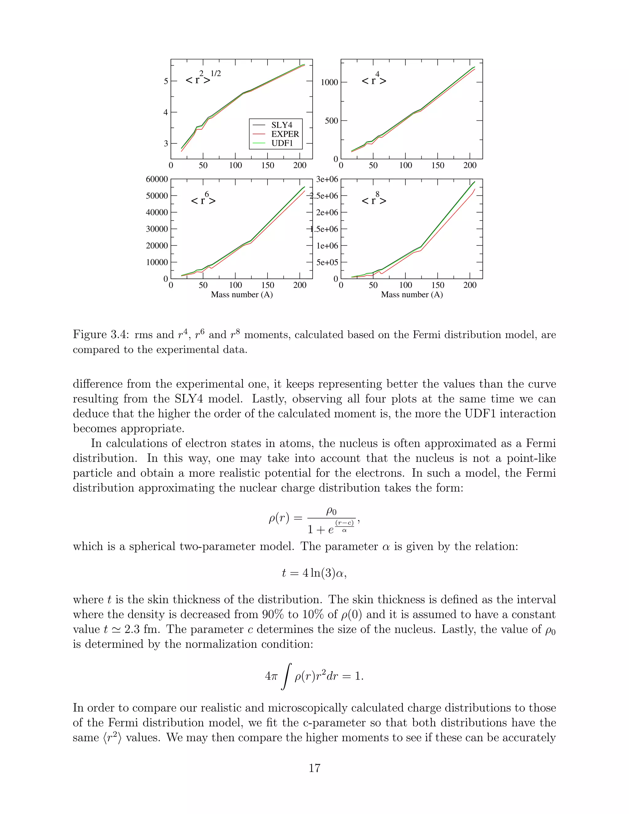
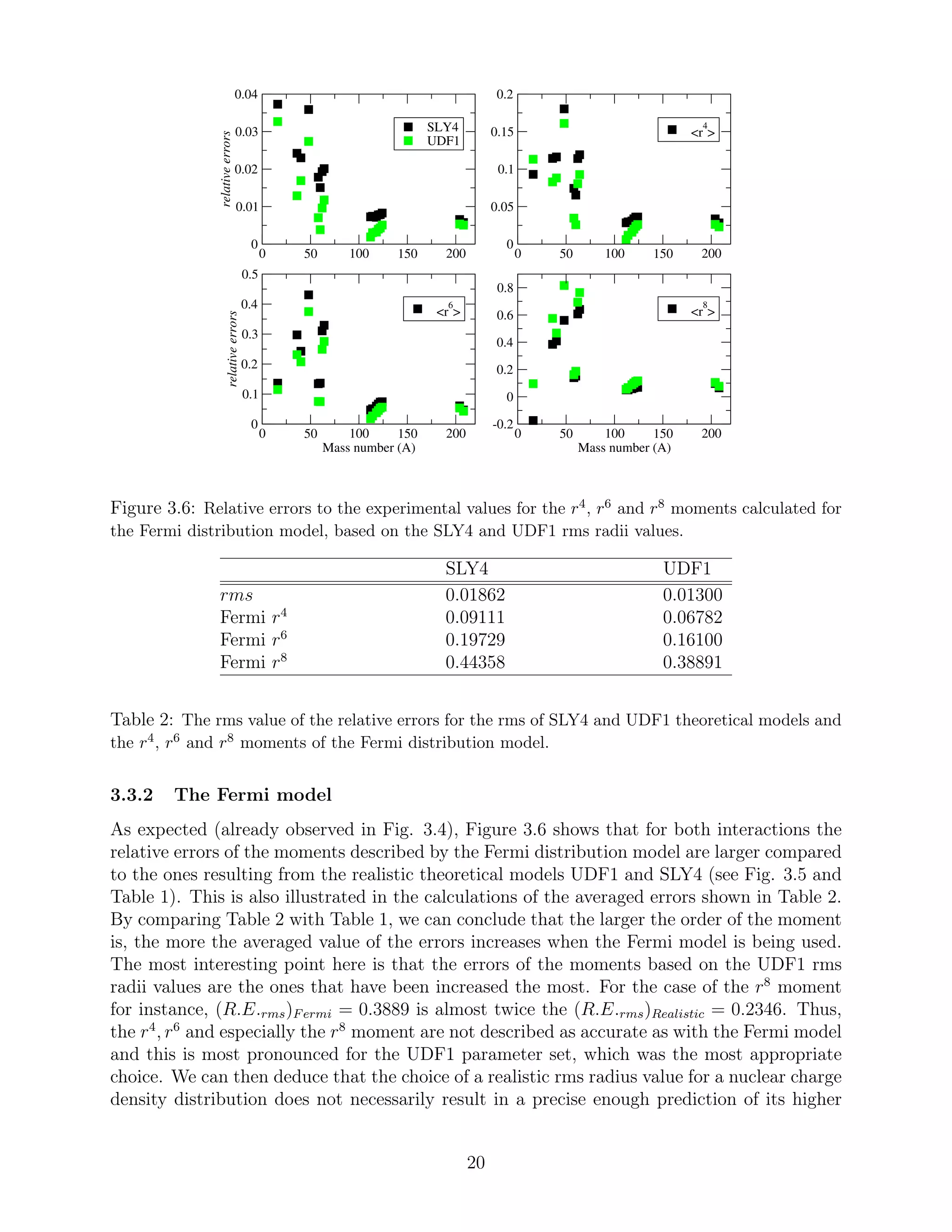
described by the Fermi distribution. The results are displayed in Figure 3.4. Although the
r2
values are identical to the ones from the realistic HFB calculations, they are again shown
in this figure.
As seen in Figure 3.4, the use of different rms radii values (based on the SLY4 and
UDF1 calculations respectively) do not result in observable differences in the values of the
higher order moments, once the Fermi model is used in both cases to calculate them. Hence,
the black and green curves are almost identical in the r4
-, r6
- and r8
-moment plots.
Comparing Figure 3.4 to Figure 3.3, we deduce that the higher moments described by the
Fermi distribution present a larger difference from the experimental curve than the ones
predicted by the realistic SLY4 and UDF1 models. Therefore, the Fermi approximation of
the nuclear charge density distributions cannot represent the experimental data equally well,
especially when it comes to the r6
and r8
higher moments.
3.3 Accuracy of theoretical models
In this subsection we discuss the validity of the Skyrme nuclear interactions by demonstrating
their relative, to the experimental values, errors (R.E.) of rms radius, as well as r4
, r6
and
r8
moments. These are given by:
R.E. =
rN
theor − rN
exp
rN
exp
=
∆ rN
rN
exp
,
for N = 2, 4, 6 and 8 respectively. These errors are calculated for both the realistic HFB and
Fermi distributions and are discussed in subsections 3.3.1 and 3.3.2, respectively. In addition,
the rms values of these relative errors:
R.E.rms =
1
K


K
i=1
rN
i − rN
exp i
rN
exp i
2


have been calculated for all moments of both interactions and are also presented. K is the
total number of the isotopes studied, that is K = 16. Hence, a comparison between the SLY4
and UDF1 models can easier be carried out.
Lastly, the mean value of the errors for the rms radii can be compared to the corre-
sponding rms values of the typical experimental uncertainties [25]. The (R.E.RMS)exp are
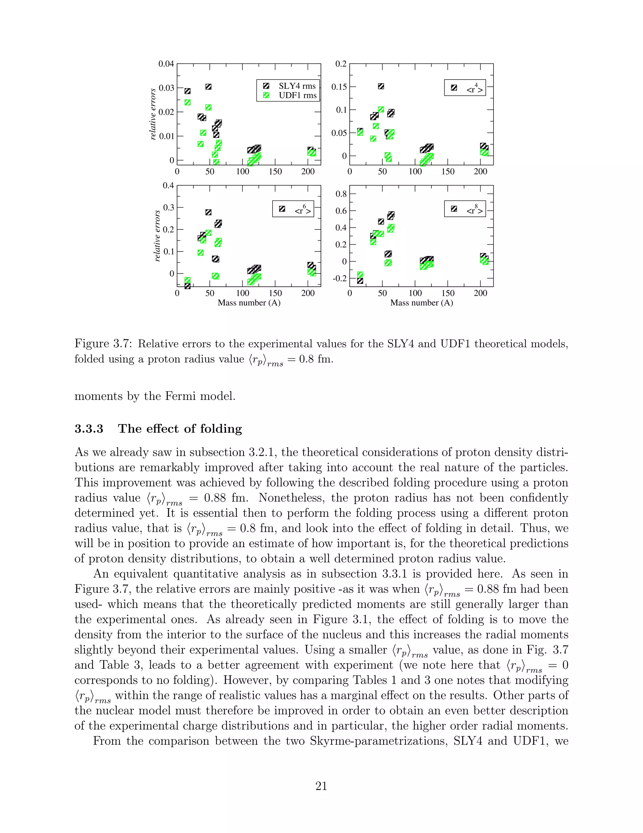
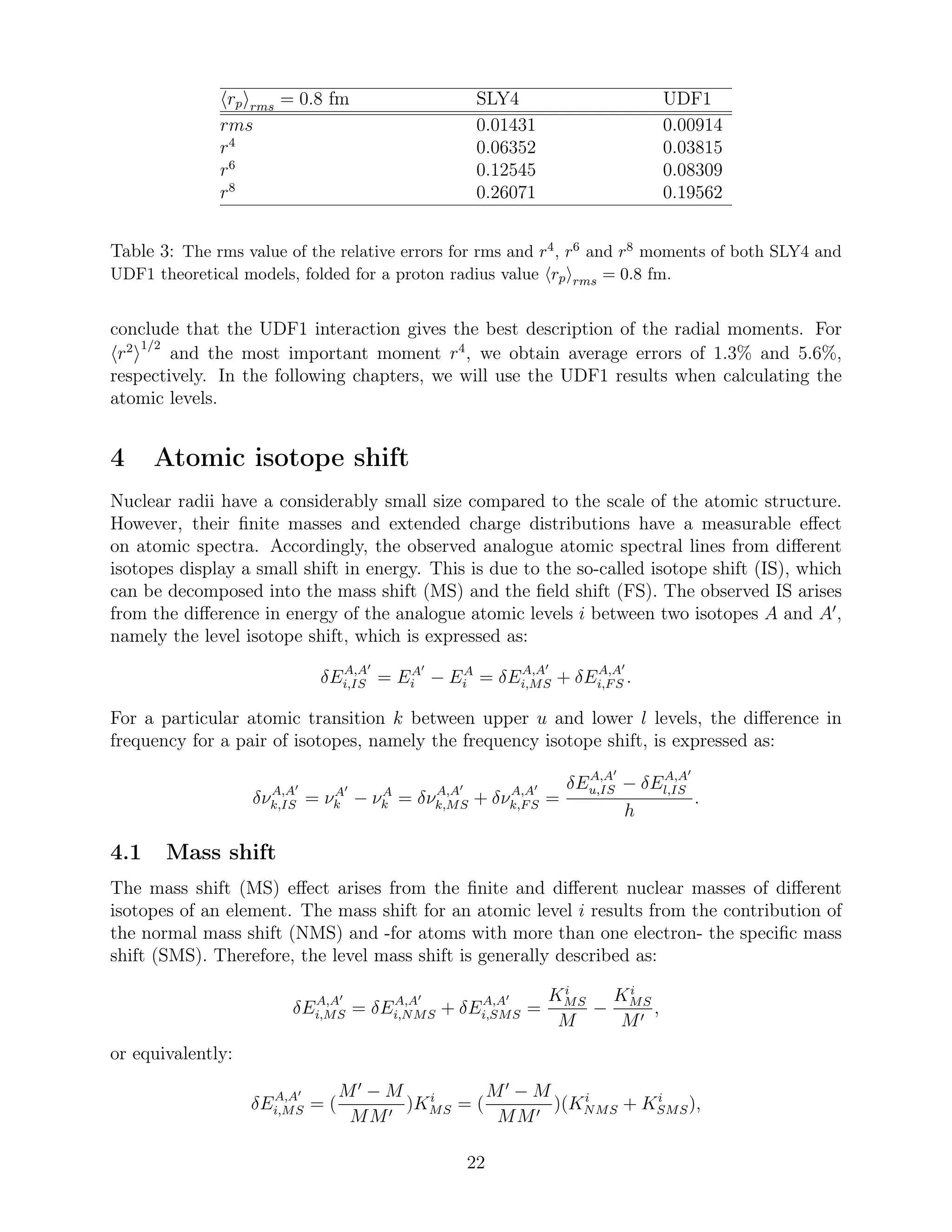
indicatively calculated for the Pb and Ni isotopes. In subsection 3.3.3, the effect of the folding
procedure for different proton radius values is discussed and thus, conclusions can be drawn
about the effect of proton radius measurements on the calculations of nuclear charge density
distributions.
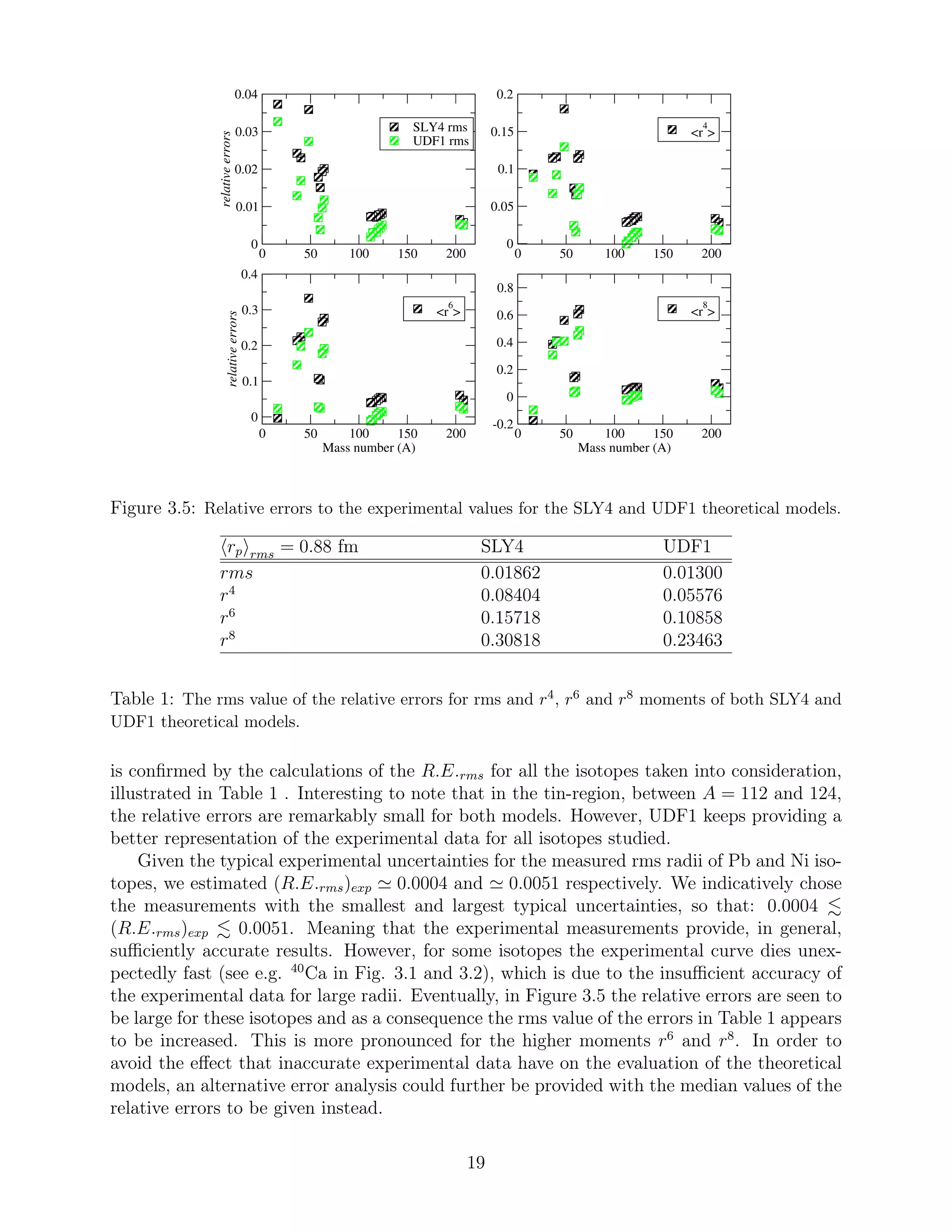
3.3.1 The realistic HFB models
Although a comparison between theoretical models and experimental measurements has al-
ready been performed in subsection 3.2.2, a quantitative analysis is also provided here in
order to highlight the appropriateness of the UDF1 set of parameters. As seen in Figure
3.5, the calculated errors for the values based on the UDF1 model are always smaller than
the ones based on the SLY4. This is valid for all four moments. Moreover, this allegation
18

0 50 100 150 200
0
0.01
0.02
0.03
0.04
relativeerrors
SLY4 rms
UDF1 rms
0 50 100 150 200
0
0.05
0.1
0.15
0.2
<r
4
>
0 50 100 150 200
Mass number (A)
0
0.1
0.2
0.3
0.4
relativeerrors
<r
6
>
0 50 100 150 200
Mass number (A)
-0.2
0
0.2
0.4
0.6
0.8
<r
8
>
Figure 3.5: Relative errors to the experimental values for the SLY4 and UDF1 theoretical models.
rp rms = 0.88 fm SLY4 UDF1
rms 0.01862 0.01300
r4
0.08404 0.05576
r6
0.15718 0.10858
r8
0.30818 0.23463
Table 1: The rms value of the relative errors for rms and r4, r6 and r8 moments of both SLY4 and
UDF1 theoretical models.
is confirmed by the calculations of the R.E.rms for all the isotopes taken into consideration,
illustrated in Table 1 . Interesting to note that in the tin-region, between A = 112 and 124,
the relative errors are remarkably small for both models. However, UDF1 keeps providing a
better representation of the experimental data for all isotopes studied.
Given the typical experimental uncertainties for the measured rms radii of Pb and Ni iso-
topes, we estimated (R.E.rms)exp ≃ 0.0004 and ≃ 0.0051 respectively. We indicatively chose
the measurements with the smallest and largest typical uncertainties, so that: 0.0004
(R.E.rms)exp 0.0051. Meaning that the experimental measurements provide, in general,
sufficiently accurate results. However, for some isotopes the experimental curve dies unex-
pectedly fast (see e.g. 40
Ca in Fig. 3.1 and 3.2), which is due to the insufficient accuracy of
the experimental data for large radii. Eventually, in Figure 3.5 the relative errors are seen to
be large for these isotopes and as a consequence the rms value of the errors in Table 1 appears
to be increased. This is more pronounced for the higher moments r6
and r8
. In order to
avoid the effect that inaccurate experimental data have on the evaluation of the theoretical
models, an alternative error analysis could further be provided with the median values of the
relative errors to be given instead.
19

0 50 100 150 200
0
0.01
0.02
0.03
0.04
relativeerrors
SLY4
UDF1
0 50 100 150 200
0
0.05
0.1
0.15
0.2
<r
4
>
0 50 100 150 200
Mass number (A)
0
0.1
0.2
0.3
0.4
0.5
relativeerrors
<r
6
>
0 50 100 150 200
Mass number (A)
-0.2
0
0.2
0.4
0.6
0.8
<r
8
>
Figure 3.6: Relative errors to the experimental values for the r4, r6 and r8 moments calculated for
the Fermi distribution model, based on the SLY4 and UDF1 rms radii values.
SLY4 UDF1
rms 0.01862 0.01300
Fermi r4
0.09111 0.06782
Fermi r6
0.19729 0.16100
Fermi r8
0.44358 0.38891
Table 2: The rms value of the relative errors for the rms of SLY4 and UDF1 theoretical models and
the r4, r6 and r8 moments of the Fermi distribution model.
3.3.2 The Fermi model
As expected (already observed in Fig. 3.4), Figure 3.6 shows that for both interactions the
relative errors of the moments described by the Fermi distribution model are larger compared
to the ones resulting from the realistic theoretical models UDF1 and SLY4 (see Fig. 3.5 and
Table 1). This is also illustrated in the calculations of the averaged errors shown in Table 2.
By comparing Table 2 with Table 1, we can conclude that the larger the order of the moment
is, the more the averaged value of the errors increases when the Fermi model is being used.
The most interesting point here is that the errors of the moments based on the UDF1 rms
radii values are the ones that have been increased the most. For the case of the r8
moment
for instance, (R.E.rms)Fermi = 0.3889 is almost twice the (R.E.rms)Realistic = 0.2346. Thus,
the r4
, r6
and especially the r8
moment are not described as accurate as with the Fermi model
and this is most pronounced for the UDF1 parameter set, which was the most appropriate
choice. We can then deduce that the choice of a realistic rms radius value for a nuclear charge
density distribution does not necessarily result in a precise enough prediction of its higher
20

0 50 100 150 200
0
0.01
0.02
0.03
0.04
relativeerrors
SLY4 rms
UDF1 rms
0 50 100 150 200
0
0.05
0.1
0.15
0.2
<r
4
>
0 50 100 150 200
Mass number (A)
0
0.1
0.2
0.3
0.4
relativeerrors
<r
6
>
0 50 100 150 200
Mass number (A)
-0.2
0
0.2
0.4
0.6
0.8
<r
8
>
Figure 3.7: Relative errors to the experimental values for the SLY4 and UDF1 theoretical models,
folded using a proton radius value rp rms = 0.8 fm.
moments by the Fermi model.
3.3.3 The effect of folding
As we already saw in subsection 3.2.1, the theoretical considerations of proton density distri-
butions are remarkably improved after taking into account the real nature of the particles.
This improvement was achieved by following the described folding procedure using a proton
radius value rp rms = 0.88 fm. Nonetheless, the proton radius has not been confidently
determined yet. It is essential then to perform the folding process using a different proton
radius value, that is rp rms = 0.8 fm, and look into the effect of folding in detail. Thus, we
will be in position to provide an estimate of how important is, for the theoretical predictions
of proton density distributions, to obtain a well determined proton radius value.
An equivalent quantitative analysis as in subsection 3.3.1 is provided here. As seen in
Figure 3.7, the relative errors are mainly positive -as it was when rp rms = 0.88 fm had been
used- which means that the theoretically predicted moments are still generally larger than
the experimental ones. As already seen in Figure 3.1, the effect of folding is to move the
density from the interior to the surface of the nucleus and this increases the radial moments
slightly beyond their experimental values. Using a smaller rp rms value, as done in Fig. 3.7
and Table 3, leads to a better agreement with experiment (we note here that rp rms = 0
corresponds to no folding). However, by comparing Tables 1 and 3 one notes that modifying
rp rms within the range of realistic values has a marginal effect on the results. Other parts of
the nuclear model must therefore be improved in order to obtain an even better description
of the experimental charge distributions and in particular, the higher order radial moments.
From the comparison between the two Skyrme-parametrizations, SLY4 and UDF1, we
21

rp rms = 0.8 fm SLY4 UDF1
rms 0.01431 0.00914
r4
0.06352 0.03815
r6
0.12545 0.08309
r8
0.26071 0.19562
Table 3: The rms value of the relative errors for rms and r4, r6 and r8 moments of both SLY4 and
UDF1 theoretical models, folded for a proton radius value rp rms = 0.8 fm.
conclude that the UDF1 interaction gives the best description of the radial moments. For
r2 1/2
and the most important moment r4
, we obtain average errors of 1.3% and 5.6%,
respectively. In the following chapters, we will use the UDF1 results when calculating the
atomic levels.
4 Atomic isotope shift
Nuclear radii have a considerably small size compared to the scale of the atomic structure.
However, their finite masses and extended charge distributions have a measurable effect
on atomic spectra. Accordingly, the observed analogue atomic spectral lines from different
isotopes display a small shift in energy. This is due to the so-called isotope shift (IS), which
can be decomposed into the mass shift (MS) and the field shift (FS). The observed IS arises
from the difference in energy of the analogue atomic levels i between two isotopes A and A′
,
namely the level isotope shift, which is expressed as:
δEA,A′
i,IS = EA′
i − EA
i = δEA,A′
i,MS + δEA,A′
i,FS .
For a particular atomic transition k between upper u and lower l levels, the difference in
frequency for a pair of isotopes, namely the frequency isotope shift, is expressed as:
δνA,A′
k,IS = νA′
k − νA
k = δνA,A′
k,MS + δνA,A′
k,FS =
δEA,A′
u,IS − δEA,A′
l,IS
h
.
4.1 Mass shift
The mass shift (MS) effect arises from the finite and different nuclear masses of different
isotopes of an element. The mass shift for an atomic level i results from the contribution of
the normal mass shift (NMS) and -for atoms with more than one electron- the specific mass
shift (SMS). Therefore, the level mass shift is generally described as:
δEA,A′
i,MS = δEA,A′
i,NMS + δEA,A′
i,SMS =
Ki
MS
M
−
Ki
MS
M′
,
or equivalently:
δEA,A′
i,MS = (
M′
− M
MM′
)Ki
MS = (
M′
− M
MM′
)(Ki
NMS + Ki
SMS),
22

where M and M′
are the atomic masses of the isotopes and Ki
NMS, Ki
SMS the mass-
independent, nuclear recoil normal and specific mass shift parameters [14] [24] [21]. The
corresponding line frequency isotope mass shift can then be written as:
δνA,A′
k,MS = δνA,A′
k,NMS + δνA,A′
k,SMS,
with
δνA,A′
k,MS = (
M′
− M
MM′
)
∆KMS
h
= (
M′
− M
MM′
)∆ ˜KMS,
where ∆KMS = ∆KNMS + ∆KSMS. Now, ∆KMS = (Ku
MS − Kl
MS) constitute the frequency
mass parameters for a transition k that connects the upper u and lower l level. The normal
and specific mass shift parameters are provided by the program ris3u [12] included in the
GRASP2K package. Hence, together with available nuclear mass data, isotope-dependent
energies and total isotope mass shifts are determined. The mass shift effect is dominant in
light systems, whereas in heavier systems its contribution becomes smaller.
4.2 Field shift
The isotope field shift (FS) arises from the differences in the nuclear charge density dis-
tribution between isotopes, which is caused by the different number of neutrons. Unlike
point-like charge distributions, realistic charge distributions alter the central field that the
bound atomic electrons experience. Hence, the extended charge distributions influence the
presence of the electrons inside the nuclear volume by pulling them out. The electron energy
levels and very likely the transition energies will then be affected. Evidently, the effect of the
nuclear distributions will be more pronounced for the electrons moving in s and p orbitals.
Moreover, the heavier the nuclear systems are, the more the electrons are pulled out and the
greater the FS becomes.
4.2.1 Variational approach
In the GRASP2K package [11], the multi-configuration Dirac-Hartree-Fock (MCDHF) method
provides an approximate solution of the atomic wave-functions. This method is the so-called
variational approach (VA), based on the minimization process of the total energy of the sys-
tem according to the variational principle (see chapter 2). Since in these calculations the
nucleus is assumed to have infinite mass, there is no MS effect contribution. Therefore, by
performing separate MCDHF calculations for two isotopes A and A′
with different parameter
set describing the respective charge distributions, the level field shift of an atomic level i is
calculated as:
δEA,A′
i,FS = EA′
i − EA
i ,
and consequently, the frequency transition field shift for a certain transition k will be given
by:
δνA,A′
k,FS ≡ νA′
k − νA
k =
δEA,A′
k,FS
h
,
where the difference δEA,A′
k = δEA,A′
u − δEA,A′
l is called transition field shift between the
chosen, upper u and lower l, levels. This method is highly model-dependent, since the shape of
the nucleus is approximated by a spherical two-parameter Fermi model (see subsection 3.2.2)
23

in GRASP2K. Namely, the higher than r2
moments that determine the shape of the nuclear
charge distribution are predicted by a Fermi distribution having a diffuseness parameter
t = 2.3 fm and a radius parameter c tuned to reproduce the desired r2
moment. However,
the implementation of MCDHF provides the “exact” method for estimating the frequency
field shifts, serving as a benchmark when comparing to different perturbative approaches
below.
4.2.2 Perturbative methods
As seen in 4.2.1, the “exact” level field shifts are obtained by subtracting one atomic level
energy from another, which results in a tiny difference compared to the magnitude of the
undisturbed level energies Ei. Therefore, an alternative approach based on the first-order
perturbation theory may be used, so that the first-order level field shift of a level i can be
written as:
δE
(1)A,A′
i,FS = −
R3
[VA′ (r) − VA(r)]ρe
i (r)d3
r,
where VA(r) and VA′ (r) are the one-electron potentials arising from the different nuclear
charge distributions for the two isotopes A and A′
and ρe
i (r) is the electron density distribution
within the nuclear volume of the reference isotope A. In the theoretical considerations of
frequency field shifts, it is often assumed that the electron density is constant within the
nucleus, that is ρe
i (r) = ρe
i (0). The level and frequency field shifts can then roughly be
estimated as:
δE
(1)A,A′
i,FS ≈
2π
3
Zρe
i (0)δ r2 A,A′
= ̥i,1δ r2 A,A′
and
δν
(1)A,A′
k,FS ≈
Z
3
∆ρe
k(0)δ r2 A,A′
= Fk,1δ r2 A,A′
,
where ∆ρe
k(0) = ρe
u(0) − ρe
l (0) and ̥i,1, Fk,1 are the so-called electronic factors. Thus, the
field shift depends only on the difference between the second radial nuclear moments of the
chosen pair of isotopes.
This approximation works well as long as the atomic number is not too large. However,
in heavier systems, a reformulation of the field shift is needed, where the shape of the elec-
tron density inside the nucleus is taken into account. Assuming extended nuclear charge
distributions, it can be shown that the electron density to a very good approximation can be
expanded, around r = 0, as an even polynomial function:
ρe
i (r) ≈ b(r) = bi,1 + bi,2r2
+ bi,3r4
+ bi,4r6
,
so that the first-order level field shift is given by the expansion [12] [20] [5] [10]:
δE
(1)A,A′
i,FS =
4
N=1
̥i,N δ r2N A,A′
,
where the level electronic factors now are ̥i,N = 2π
N(2N+1)
Zbi,N for a certain atomic number
Z and δ r2N A,A′
= r2N A′
− r2N A
are the differences of the nuclear radial moments, of
24

order 2N for N = 1, 2, 3 and 4, for isotopes A, A′
. Accordingly, the first-order frequency field
shift will be given by:
δν
(1)A,A′
k,FS =
4
N=1
Fk,N δ r2N A,A′
,
where Fk,N = 1
N(2N+1)
Z∆bk,N are the frequency electronic factors, related to the change in
the electronic density inside the nucleus, with ∆bk,N = bu,N − bl,N defining the difference of
the polynomial function coefficients between the upper u and the lower l level.
The electron density ρe
(r) is constructed using ris3u [12] [10], one of the GRASP2K
programs. Subsequently, this density is fitted to the polynomial function b(r) so that the
coefficients bi,N and their differences ∆bk,N can be calculated. Finally, the level and frequency
electronic factors, ̥i and Fk,N , are deduced for the reference isotope A. This approach is
not constrained to any approximated model describing the nuclear charge density distribu-
tions. Therefore, the realistic nuclear radial moments extracted from the Skyrme-type UDF1
interaction can be used in order to estimate the frequency shifts for several transitions and
isotope pairs.
4.2.3 Validation of perturbative method
Since the variational approach stands so far for the best approximation to the field shifts,
this method will serve as the verification instrument for the newly introduced perturbative
method. The charge distributions in the VA are based on a two-parameter spherical Fermi
model. For this model we adopt the same rms radii as given in Angelis & Marinova [2] that
was used in the VA and for higher moments given by the Fermi model, should be virtually
identical.
The validation of the RFS is illustrated in Figure 4.1, for three different Lithium-like
lead isotope pairs and two different transitions k. In each pair, the 208
Pb is used as the
reference isotope A and the electronic field shift factors are deduced for this nucleus. Hence,
the frequency field shifts are plotted in relation to the mass number A′
of the non-reference
isotope. As seen in Figure 4.1, after adding all four expansion terms (red circle), the frequency
field shifts δν
(1)208,A′
k almost perfectly agree with the δν208,A′
k,V A (black square) resulting from
the variational approach described in 4.2.1. Namely, the perturbative method provides us
with rather satisfactory results. Additionally, the accumulated frequency field shift values,
δν208,A′
k, N=1,n
for n = 1, 2, 3, are displayed in the same plot for all three isotope pair combinations
208, A′
. The δν208,A′
k, N=1,n
give three different frequency field shift values after each expansion
term has been consecutively added, before the final δν
(1)208,A′
k is deduced. We notice that
for n = 1, we obtain δν208,A′
k, N=1,1
= Fk,1δ r2 208,A′
(green ring), which is the frequency field
shift estimated using the assumption of constant electron density inside the nucleus. It is
noteworthy here that the higher than second order moments evidently play an important
role in the expansion of the reformulated frequency field shift, proving that the shape of the
electron density inside such heavy nuclear systems always needs to be taken into account.
In order to perform a quantitative comparison of the contribution rate from each expansion
term, the isolated term contributions are presented in Table 4 for the isotope pair 208,200
Pb.
The accumulated contributions and contribution percentages are also displayed. As seen
in Table 4, the terms that include the nuclear radial moments differences δ r2N 208,200
for
25

190 195 200 205 210 215
Mass number (A’)
-20000
0
20000
40000
60000
δν
208,A’
[GHz]
VA
Reformulated
1st Exp. term
2nd Exp. term
3rd Exp. term
Transition 1
190 195 200 205 210 215
Mass number (A’)
-20000
0
20000
40000
60000
Transition 2
Figure 4.1: The frequency ﬁeld shift δν208,A′
for the Li-like Pb isotope pairs with A′ = 192, 200
and 210. “Transition 1” refers to 1s22s 2S1/2+ −→ 1s22p 2P1/2− transition, while “transition 2” is
addressed to the 1s22s 2S1/2+ −→ 1s22p 2P3/2− transition. The δν208,A′
V A resulting from the vari-
ational approach (VA) calculations, as well as the accumulated frequency ﬁeld shifts δν208,A′
N=1,n
=
n
N=1
Fk,N δ r2N 208,A′
for n = 1, 2, 3, 4 resulting from the perturbative approach, are separately
demonstrated.
26

n δν208,200
n [GHz] δν208,200
N=1,n
[GHz]
δν208,200
N=1,n
δν208,200
V A
[%] δν208,200
n
δν208,200
V A
[%]
1 30895.8235 30895.8235 108.172 108.172
2 -2717.8996 28177.9239 98.656 -9.516
3 505.9503 28683.8742 100.428 1.771
4 -59.2375 28624.6367 100.220 -0.207
δν208,200
V A 28561.7494 100
Table 4: Column two contains the isolated contributions δν208,200
n = Fk,nδ r2n 208,200
that each one
out of the four in total expansion terms gives to the final
4
N=1
Fk,N δ r2N 208,200
frequency field shift
value of the 208,200Pb pair calculated for 1s22s 2S1/2+ −→ 1s22p 2P1/2− transition, whilst column
three displays the accumulated contributions δν208,200
N=1,n
=
n
N=1
Fk,N δ r2N 208,200
. The r2 values
are taken from Angelis & Marinova [2]. In column four, the matching percentage of the accumulated
contributions is estimated based on the δν208,200
V A value. Lastly, the matching percentages of the
isolated contributions are presented in column five.
N = 2, 3, 4 give almost 8% contribution to a precise evaluation of the field shifts, meaning
that the constant electron density approximation is not good enough for the description of the
heavy nuclear systems. Nonetheless, the major correction comes from the second expansion
term that takes into account the differences between the r4
moments. However, from the
values of the accumulated percentages we draw the conclusion that the expansion converges
to a slightly higher value than the one given by the δν208,200
V A . Thus, the reformulation of the
field shift remains an approximation to the “exact” VA method. The observed discrepancy
is mainly due to the fact that the same electron density, deduced for the reference isotope
A = 208, is used in both nuclei. Other assumptions that have been made throughout the
formulation of the perturbative approach are expected to play a minor role.
5 The effect of realistic nuclear charge distributions
In chapter 4, the alternative approach introduced for estimating field shifts was validated.
This approach is rather powerful since it enables the investigation of the effect that more
realistic nuclear charge distributions have on level and frequency field shifts. In this section,
we initially focus on the magnitude of the higher order contributions in the reformulated
field shift, using theoretically predicted r4
, r6
and r8
moments. The corrections provided
by the realistic charge distributions are compared to the uncertainties of the experimentally
observed field shifts. Conclusions can then be drawn on the importance of such corrections
depending on whether or not these could be detected by making use of the current experi-
mental techniques. Ultimately, extraction of nuclear radial moment differences, δ r2N
for
N = 1, 2, 3 and 4, is discussed assuming that four independent transitions are available. How-
ever, a novel approach, where only two transitions are needed for the extraction of higher
27

order radial moments, will also be outlined.
5.1 Higher order moments in field shift
In the electronic calculations, the shape of the nuclear charge density distribution is approx-
imated by the two-parameter spherical Fermi model described in subsection 3.2.2. However,
the reformulation of the field shift enables calculations based on realistic nuclear charge dis-
tributions. Hence, the main objective in this section is to examine the magnitude of the
corrections δνrealistic − δνFermi. We fit the Fermi distribution so that it has the same r2
value as the realistic distribution. Then:
δνFermi = Fk,1δ r2
realistic
+
4
N=2
Fk,N δ r2N
Fermi
,
and
δνrealistic =
4
N=1
Fk,N δ r2N
realistic
.
Therefore, the frequency field shifts calculated using realistic charge distributions can be
equivalently written:
δνrealistic = Fk,1δ r2
realistic
+
4
N=2
Fk,N δ r2N
Fermi
+ (δνrealistic − δνFermi),
treating the correction δνrealistic − δνFermi as an additional term. For spherical nuclei, the
realistic nuclear radial moments are extracted from the charge density distributions described
by the Skyrme-based UDF1 interaction (see chapter 3). For deformed nuclei the realistic
nuclear moments are calculated with the same interaction using the program HFBTHO
(2.00d) [22].
We focus on heavy nuclear systems where the splitting of the energy values and transitions
are larger. Besides, it is in these systems where the higher order moments contribute to a
considerable extent. The orbitals that are affected the most by the change in the nuclear
charge distributions between the isotopes are the ones closest to the nucleus. Therefore,
transitions exclusively between s and p orbitals are examined here.
5.1.1 Spherical nuclei
The contribution from the “correction term” δνrealistic − δνFermi is plotted in Figure 5.1 for a
variety of Lithium-like systems with spherical nuclei. The Li-like system of lead Pb79+
, for
which several isotope pair combinations have been studied, is of main interest. As seen in
Figure 5.1, the absolute magnitude of the “correction term” mainly depends on the difference
between the neutron number ∆N208,A′
(or equivalently the difference between the mass num-
ber ∆A208,A′
) for the isotopes 208, A′
of the chosen pair. The larger the difference ∆N208,A′
is, the more important the role of the corrections becomes. When more neutrons are added
it is expected that they will pull out the protons, leading to an increased diffuseness of the
distribution. This effect is not included in the Fermi model and may be a reason for the
28

100 150 200 250 300
Mass number (A’)
-200
-100
0
100
200
(δνrealistic
−δνFermi
)[GHz]
120,A’
Sn
208,A’
Pb
198,194
Er
304,300
Uuh
∆N
208,A’
= 24
∆Ν
208,Α
= 2
208
Pb120
Sn
Figure 5.1: The corrections δνrealistic − δνFermi to the frequency ﬁeld shift calculations in relation
to the mass number A′ of the non-reference isotope. The results for the Li-like lead Pb79+ isotope
pairs 208,A′
Pb for A′ = 184, 192, 200, 210 and 214 are illustrated in blue and the ones for the Li-like
tin, 120,114Sn and 120,126Sn, in black. The reference isotopes used in these pair combinations, 208Pb
and 120Sn, are pointed out with red. The result for the Li-like ununhexium pair 300,304Uuh is shown
in green. All plotted values refer to the transition 1s22s 2S1/2+ −→ 1s22p 2P1/2− .
29

n δν208,200
n [GHz] δν208,200
N=1,n
[GHz]
δν208,200
N=1,n
δν208,200
N=1,5
[%] δν208,200
n
δν208,200
N=1,5
[%]
1 35965.7809 35965.7809 108.205 108.205
2 -3210.1387 32755.6422 98.547 -9.658
3 599.4241 33355.0663 100.351 1.804
4 -70.7353 33284.3311 100.138 -0.203
5 -45.8809 33238.4501 100 -0.138
Table 5: Column two contains the isolated contributions δν208,200
n to the final frequency field shift
value of the 208,200Pb pair and the transition 1s22s 2S1/2+ −→ 1s22p 2P1/2− . For n = 1, 2, 3 and
4, δν208,200
n = Fk,nδ r2n 208,200
are given by the expansion terms of the reformulated frequency
field shift. The δ r2 is given by the realistic rms radii values of the isotopes, based on the UDF1
interaction, while δ r2N for n = 2, 3, 4 are given by the higher moments reproduced using a Fermi
model that is formed on the UDF1 rms radii. Lastly, δν208,200
5 represents the “correction term”
δνrealistic − δνFermi. Column three displays the accumulated contributions δν208,200
N=1,n
, with δν208,200
N=1,5
being the δνrealistic. In column four, the matching percentage of the accumulated contributions is
estimated based on the final δνrealistic value, whilst column five contains the matching percentages
of the isolated contributions.
observed difference. However, these corrections are tiny for the much lighter system of (Li-
like) Tin. In order to stress the larger magnitude of the effect that realistic higher order
nuclear moments have on the frequency field shift estimated in heavy systems, the value of
δνrealistic − δνFermi has been calculated for the extreme case of the superheavy neutron-rich
ununhexium element of proton number Z = 116. As seen in Figure 5.1, even for the small
change ∆N = 4, the corrections in superheavy systems can be hundred times larger than the
ones in lighter systems.
A quantitative analysis of the magnitude of the “correction term” δνrealistic − δνFermi, as
well as its contribution percentage to the final realistic frequency field shift value δνrealistic
for the isotope pair 208,200
Pb is displayed in Table 5. As seen in Table 5, the additional term
δνrealistic − δνFermi gives ≃ 0.14% contribution, which is smaller than the one resulting from
the fourth expansion term. However, for isotope pairs with larger ∆N, like the 208,184
Pb,
the correction adds a contribution that reaches 0.26%, which in this case is larger than
the contribution of the last expansion term (≃ 0.2%). Therefore, we deduce that even in
nuclear systems that are spherical the two-parameter Fermi model may not always provide a
satisfactory description of the higher order moments that are used in the calculations of the
RFS.
5.1.2 Deformed nuclei
The two-parameter Fermi model does not take into account the effect of deformation. As a
result, the effect of the realistic charge distributions on the field shifts is expected to be even
larger in atomic systems where the nuclei are deformed. In such systems, the axially symmet-
ric deformed Fermi model is suggested to be used instead. The nuclear charge distributions
are in this case given by:
30

100 150 200 250
Mass number (A’)
-100
0
100
200
(δνrealistic
−δνFermi
)[GHz]
142,A’
Nd
208,A’
Pb
β ~0.35
β ~0.14
208
Pb
142
Nd
120
Sn
120,A’
Sn
β ∼0.29
to the mass number A′ of the non-reference isotope. The results for the Li-like spherical lead
Pb79+ isotope pairs are illustrated in blue, while Li-like deformed neodymium Nd57+ isotope pairs
are displayed in green. For Nd57+, the magnitude of the quadrupole deformation parameter β of
the non-reference isotopes A′ is indicatively shown for two different isotope groups. The reference
isotopes used in the pair combinations, 208Pb, 142Nd and 120Sn, are all spherical and are pointed
out with red. All plotted values refer to the 1s22s 2S1/2+ −→ 1s22p 2P1/2− transition.
0 0.05 0.1 0.15 0.2 0.25 0.3 0.35 0.4
beta (β)
0
50
100
150
200
(δνrealistic
−δνFermi
)[GHz]
Nd
57+
∆N
142,A’
= 4
∆N
142,A’
= 6
to the quadrupole deformation parameter β of the non-reference A′ isotope for various Nd57+ isotope
pairs. In all pairs, the reference isotope is the spherical 142Nd. Two cases of isotope pairs 142, A′ with
the same difference ∆N142,A′
in the neutron number but different δνrealistic − δνFermi magnitude,
due to the deformation β, are indicatively stressed.
31

ρ(r, θ) =
1
1 + e
r−c(θ)
a
,
where, if only quadrupole deformation is considered, c(θ) = c0[1+β20Y20(θ)]. The “correction
term” δνrealistic − δνFermi can now be decomposed into two parts and written as:
δνrealistic − δνFermi = δνrealistic − δνdef
Fermi + δνdef
Fermi − δνsph
Fermi .
The δνdef
Fermi − δνsph
Fermi part isolates the magnitude of the effect of deformation, while the
δνrealistic − δνdef
Fermi part gives the magnitude of the corrections due to other effects, like for
instance the density wiggles and the varied diffuseness that are not taken into account in the
simplified Fermi approximation. In order to separately estimate the effect of deformation,
we additionally calculated the frequency field shifts based on the higher order moments that
are predicted by the deformed Fermi model. The deformed Fermi model is for each nuclear
system developed based on a certain quadrupole deformation parameter β, in addition to the
realistic rms radius of the nucleus, which is theoretically predicted by the HFBTHO (2.00d)
program.
The Li-like system of neodymium is of great interest since the theoretically calculated
frequency field shifts can be further compared to the available experimental data. There-
fore, in Figure 5.2, the contribution to the frequency field shifts from the “correction term”
δνrealistic − δνFermi in relation to the mass number A′
of the non-reference isotope is plotted
for a variety of ion pairs Nd57+
, in addition to the Pb79+
and Sn47+
pairs plotted in Figure 5.1.
While the reference isotope 142
Nd is spherical, the non-reference isotope is always deformed
to a certain extent. As seen in Figure 5.2, the corrections become significant and comparable
to the heavy Li-like system of lead whenever the value of the deformation parameter β for
the non-reference isotope is large. On the other hand, in light systems and when the nuclei
have approximately spherical shape the δνrealistic − δνFermi value is negligible. This ascer-
tainment has been already highlighted for the Li-like system of tin, where all isotopes in the
pair combinations are purely spherical and as a consequence δνrealistic − δνFermi ≃ 0.
The magnitude of δνrealistic − δνFermi in relation to the deformation parameter β of the
non-reference isotope is plotted for the Nd57+
ion pairs in Figure 5.3. As seen in Figure 5.3,
there is roughly a quadratic increase of the δνrealistic − δνFermi value with the deformation.
Therefore, in lighter and deformed nuclear systems, we deduce that the change in the neutron
number ∆NA,A′
between two isotopes is not as an important factor for the estimation of the
correction δνrealistic − δνFermi as it is in the heavier systems.
In order to be able to draw conclusions about the significance of the “correction term”
in comparison to the magnitude of each one of the expansion terms, as well as the total
frequency field shift value δνrealistic, a quantitative analysis based on the isotope pair 142,150
Nd
is displayed in Table 6. Table 6 provides a similar illustration of the contributions and the
contribution percentages from each term as Table 5 does in 5.1.2. As seen in Table 6, the
term δνrealistic − δνFermi adds a contribution of ≃ 1.16% to the formulation of the frequency
field shift δνrealistic. The contribution of the corrections provided by the usage of realistic
nuclear data is now larger than the contribution from the third and fourth expansion terms
when they are summed up, which reaches ≃ 1.03%. More specifically, the major contribution
comes from the δν142,150
5 term, that is due to the usage of the deformed Fermi model. Further
on, the δν142,150
6 term, which is due to the wiggles, the skin diffuseness etc. of the realistic
32

n δν142,150
n [GHz] δν142,150
N=1,n
[GHz]
δν142,150
N=1,n
δν142,150
N=1,6
[%] δν142,150
n
δν142,150
N=1,6
[%]
1 -12979.2841 -12979.2841 105.609 105.609
2 647.7010 -12331.5831 100.339 -5.270
3 -113.5695 -12445.1526 101.263 0.924
4 12.6588 -12432.4937 101.160 -0.103
5 104.7742 -12327.7195 100.316 -0.844
6 37.8273 -12289.8922 100 -0.316
Table 6: In column two the isolated contributions δν142,150
n to the final frequency field shift value
of the 142,150Nd57+ pair calculated for 1s22s 2S1/2+ −→ 1s22p 2P1/2− transition are shown. For
n = 1, 2, 3 and 4, δν142,150
n = Fk,nδ r2n 142,150
are given by the expansion terms of the refor-
mulated frequency field shift. The δ r2 are given by the theoretically calculated rms radii of
the isotopes, while δ r2N for n = 2, 3, 4 are given by the higher moments reproduced using the
spherical two-parameter Fermi model that is formed on the theoretical rms radii. Lastly, the sum
δν142,150
5 +δν142,150
6 represents the correction δνrealistic−δνFermi, where δν142,150
5 = δνdef
Fermi−δνsph
Fermi
and δν142,150
6 = δνrealistic −δνdef
Fermi. Column three displays the accumulated contributions δν142,150
N=1,n
,
with δν142,150
N=1,6
being the δνrealistic. In column four, the matching percentage of the accumulated con-
tributions is estimated based on the final δνrealistic value, whilst column five contains the matching
percentages of the isolated contributions.
distributions, adds a contribution of ≃ 0.32% that, as seen in Table 6, exceeds the one from
the fourth expansion term. Therefore, in deformed nuclear systems the two-parameter Fermi
model seems to be even less appropriate for the description of the r2N
, N = 2, 3 and 4,
moments than it was in the case of the spherical nuclei.
5.2 Experimental isotope shifts
The isotope shift (IS) calculations, and particularly the estimation of the corrections δνrealistic−
δνFermi to the field shifts that are provided when realistic nuclear data are used, become
more meaningful when the comparison with experimental IS observations is feasible. The
comparison of these corrections with the experimental uncertainties is also of interest since it
will reveal if the corrections should be included in the analysis and eventually if they can be
extracted from observed IS. In Li-like systems, highly accurate IS observations remain a chal-
lenge, since they are followed by relatively -compared to neutral systems- high uncertainties,
both statistical and systematic. The Li-like system of neodymium Nd57+
has been studied
and the observed isotope frequency shift is δν142,150
IS,exp = −9720(73)(145) GHz [(stat)(syst)] for
the 1s2
2s 2
S1/2+ −→1s2
2p 2
P1/2− transition and δν142,150
IS,exp = −10228(290)(484) GHz for the
1s2
2s 2
S1/2+ −→1s2
2p 2
P3/2− transition [9]. The mass shift contribution is mainly significant
in lighter systems. However, in order to obtain a reliable estimate of the “observed” frequency
field shift, subtraction of the MS component is required. For the same transitions, the total
mass shift, in the same work, were calculated to be δν142,150
MS = −387 GHz and δν142,150
MS = −435
GHz. Hence, the estimated “observed” field shift is finally δν142,150
FS,exp = −10107(73)(145) GHz
33

and δν142,150
FS,exp = −10663(290)(484) GHz, for each transition, respectively.
As seen in Table 6, for the 1s2
2s 2
S1/2+ −→1s2
2p 2
P1/2− transition δν142,150
Fermi = −12432
GHz, which after taking into account the corrections δνrealistic − δνFermi = 142 GHz takes
the value δν142,150
realistic = −12290 GHz. The calculated frequency field shift approaches the
“observed” value after the “correction term” has been added, but δν142,150
realistic is still ∼ 20%
smaller than δν142,150
FS,exp . A similar difference between “observed” and theoretically predicted
frequency field shift is obtained for the 1s2
2s 2
S1/2+ −→1s2
2p 2
P3/2− transition. Considering
the differences between experimental and theoretical rms radii, the large difference between
the corresponding frequency field shift values is not surprising. From the Angelis & Marinova
compilation [2] we obtain δ r2 142,150
exp = 1.27 fm2
, whereas the HFBTHO calculations result in
δ r2 142,150
realistic = 1.64 fm2
(∼ 20% larger). The calculated charge distributions are not expected
to be 100% exact when it comes to rms radii and particularly δ r2
values. However, they
should be realistic in terms of nuclear shapes and deformation and thus providing a more
representative description of the higher order moments.
In the particular case of 142,150
Nd where the target isotope 150
Nd is deformed, the cor-
rection is δνrealistic − δνFermi = 142 GHz > 73 GHz, which is the magnitude of the sta-
tistical uncertainty in the measurement of the δν142,150
IS,exp . The role of the “correction term”
δνrealistic − δνFermi is even more stressed when the higher moments differences δ r2N
are
extracted from the observed IS. Taking δν142,150
FS,exp = −10107(73)(145) GHz for the 1s2
2s
2
S1/2+ −→1s2
2p 2
P1/2− transition, we can extract δ r2
assuming a linear dependence:
δν142,150
FS,exp ≃ Cδ r2
.
The constant C for this particular transition is estimated using GRASP2K. We performed
separate MCDHF calculations for 142
Nd ( r2 1/2
= 4.9118 fm2
) and 150
Nd ( r2 1/2
= 5.0415
fm2
), having as a reference the former isotope and using t = 2.30 fm for both isotopes. The
reformulated field shift is δν142,150
= −9745 GHz and the “effective” field shift electronic
factor becomes:
F =
δν142,150
δ r2 142,150 =
−9745
1.2909
= −7549
GHz
fm2
.
Assuming a “dummy” isotope with r2
= r2 142
+ 1.00 fm2
and calculating the relative field
shift yields an electronic factor F′
that has almost the same magnitude as the one calculated
before so that F′
≃ F. Therefore, we can, to a good enough approximation, assume that
F = C and rely on the linearity of the field shift parameter in GHz/fm2
. Using the “observed”
field shift, we obtain:
δ r2
=
δν142,150
FS,exp
F
= 1.3389fm2
.
By taking into account the effect of the realistic charge distribution, the field shift electronic
factor takes the value:
Fcor = F +
δνrealistic − δνFermi
δ r2
realistic
= −7462
GHz
fm2
.
Using again the “observed” field shift, we obtain:
δ r2
cor
=
δν142,150
FS,exp
Fcor
= 1.3545fm2
.
34

In the work by Brandau et al. [9], the extracted δ r2
for the same transition is 1.36(1)(3) fm2
.
The δ r2
and δ r2
cor that we estimated above are slightly different due to the fact that some
small corrections from additional effects have been neglected throughout our calculations of
the “observed” field shift, whereas in the analysis of Brandau these effects have been taken
into account and subtracted from the observed IS δν142,150
IS,exp . The difference between the δ r2
and the δ r2
cor is ∼ 0.016 fm2
, which is larger than the statistical error but smaller than
the systematical error. Hence, in this case the effect from the realistic charge distributions
is important and comparable in magnitude to the observed uncertainty. It is possible to
double-check the δ r2
value by using the observed IS of the second available transition
and calculating the relevant electronic factor F, but for this transition both statistical and
systematic error are larger and thus better resolution is needed in order to see the effect of
the realistic charge distributions.
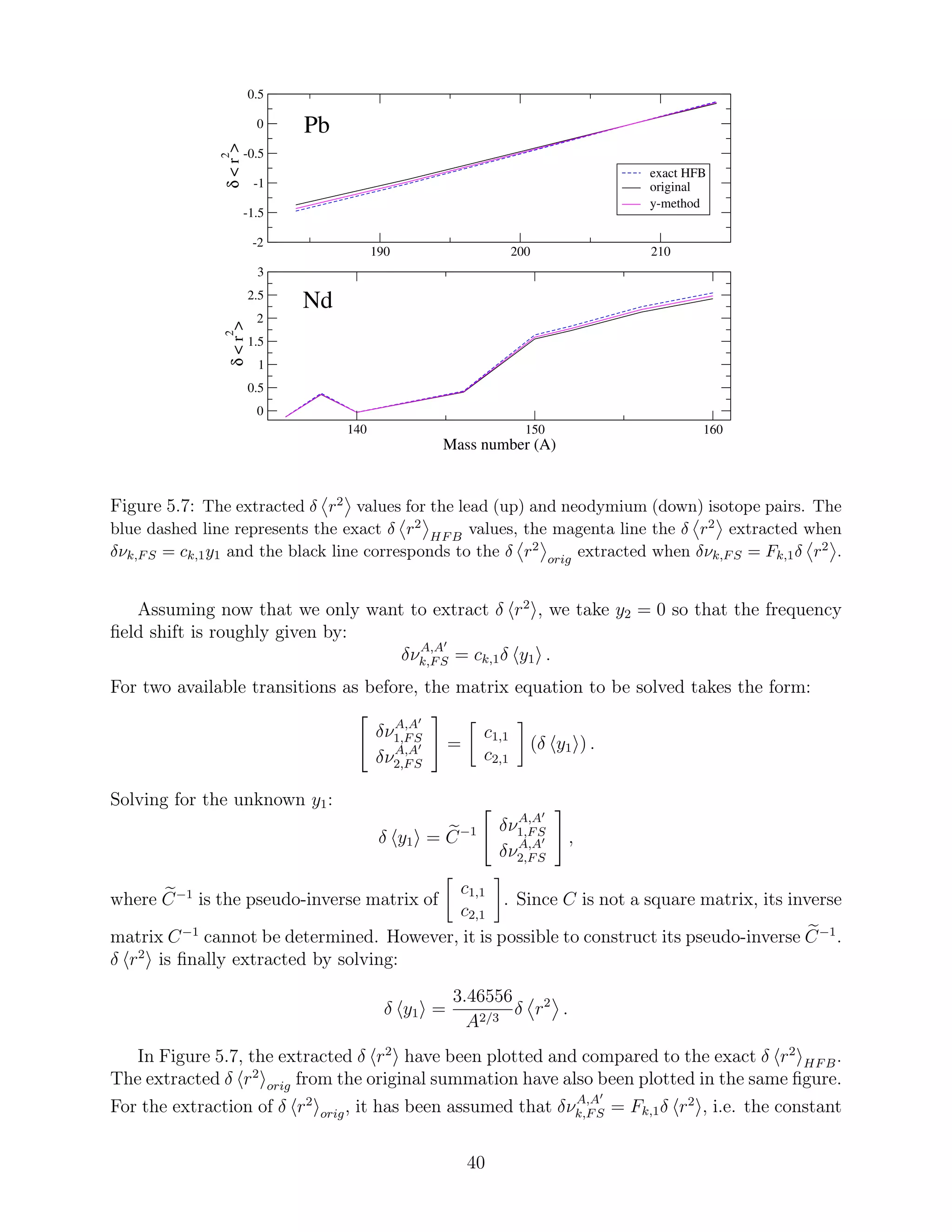
5.3 Extracting higher moments from data
The reformulation of the field shift combined with experimental isotope shifts δν
(exp)A,A′
k,IS
enables the extraction of the radial nuclear moments r2N
, N = 1, 2, 3, 4 for the target isotope
A′
, when the corresponding moments are known for the reference isotope A. Thus, conclusions
can be drawn about the nuclear shapes, deformations, density wiggles and other nuclear
properties. The extraction of all four radial moments requires four independent transitions
k to be available. A system of four equations is then solved for:
δνexp
k,IS − δνk,MS = Fk,1δ r2
+ Fk,2δ r4
+ Fk,3δ r6
+ Fk,4δ r8
,
where k = 1, 2, 3, 4. The frequency electronic factors Fk,N and the frequency mass shift
parameters ∆Kk,MS, different for each transition k, may theoretically be calculated using an
atomic structure code such as GRASP2K. However, it is rare that observed IS are available
for four transitions and in addition such systems of equations cannot be formed so that they
give trustworthy solutions for the higher than second order moments.
Looking back at Figure 4.1, we can say that the major correction, to the approximation
that assumes constant electron density ρe
i (r) = ρe
i (0), comes from the second expansion term,
i.e. Fk,2δ r4
, which takes into account the differences between the r4
moments. Nonethe-
less, the contribution from the
4
N=3
Fk,N δ r2N
part of the expression for the reformulated
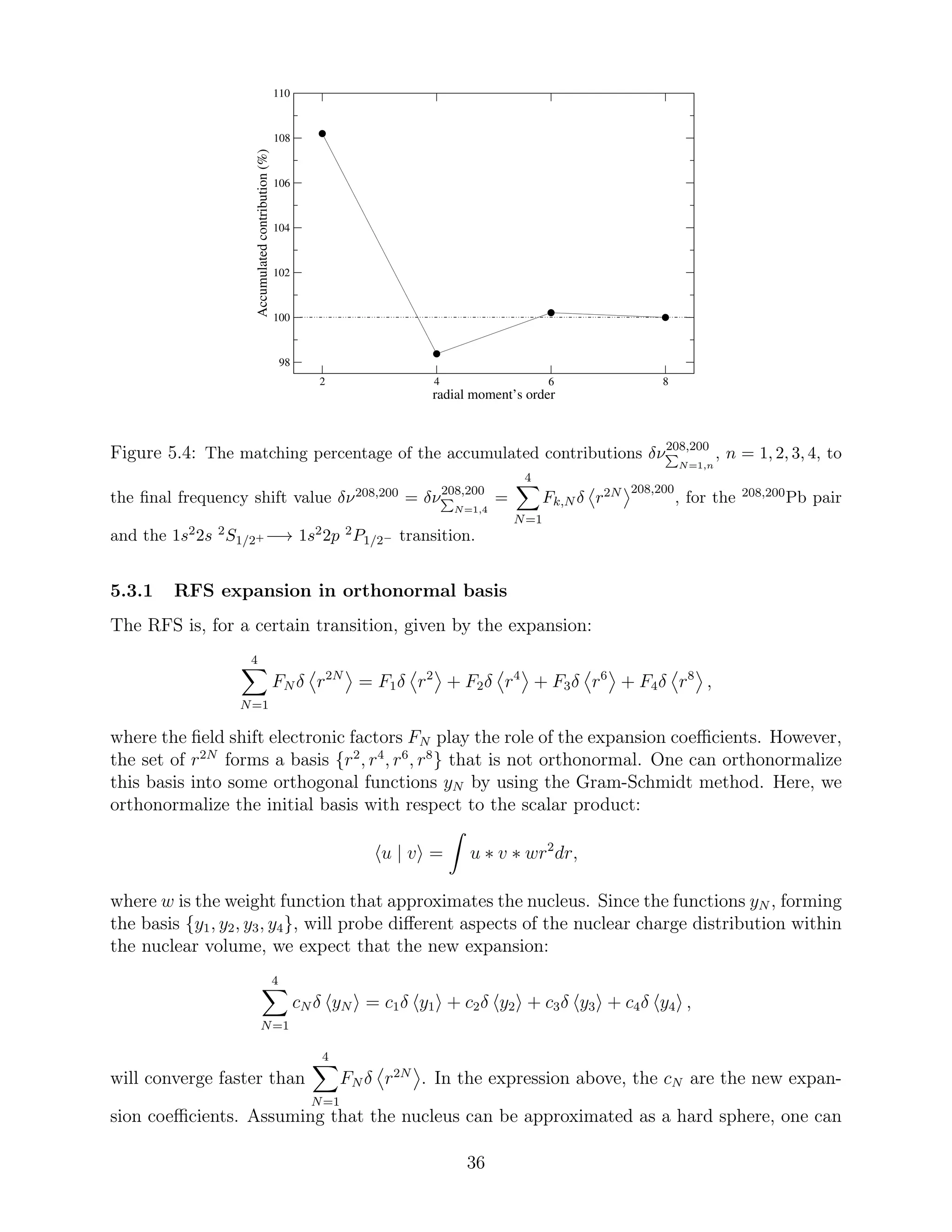
frequency field shift remains not negligible. This is also illustrated in Figure 5.4, where the
matching percentage to the final frequency shift value
4
N=1
Fk,N δ r2N 208,200
of the isotope pair
208,200
Pb has been plotted after each term is added. Obviously, when the fourth expansion
term is taken into account, the final field shift value is reached. As seen in Figure 5.4, the 4th
order radial moments add ∼ 10% contribution, the 6th moments add ∼ 2% contribution and
the last term, which contains the 8th order moments, contributes with much less. However,
a re-arrangement of the sum that gives the RFS could possibly lead to faster convergence.
35

2 4 6 8
radial moment’s order
98
100
102
104
106
108
110
Accumulatedcontribution(%)
Figure 5.4: The matching percentage of the accumulated contributions δν208,200
N=1,n
, n = 1, 2, 3, 4, to
the final frequency shift value δν208,200 = δν208,200
N=1,4
=
4
N=1
Fk,N δ r2N 208,200
, for the 208,200Pb pair
and the 1s22s 2S1/2+ −→ 1s22p 2P1/2− transition.
5.3.1 RFS expansion in orthonormal basis
The RFS is, for a certain transition, given by the expansion:
4
N=1
FN δ r2N
= F1δ r2
+ F2δ r4
+ F3δ r6
+ F4δ r8
,
where the field shift electronic factors FN play the role of the expansion coefficients. However,
the set of r2N
forms a basis {r2
, r4
, r6
, r8
} that is not orthonormal. One can orthonormalize
this basis into some orthogonal functions yN by using the Gram-Schmidt method. Here, we
orthonormalize the initial basis with respect to the scalar product:
u | v = u ∗ v ∗ wr2
dr,
where w is the weight function that approximates the nucleus. Since the functions yN , forming
the basis {y1, y2, y3, y4}, will probe different aspects of the nuclear charge distribution within
the nuclear volume, we expect that the new expansion:
4
N=1
cN δ yN = c1δ y1 + c2δ y2 + c3δ y3 + c4δ y4 ,
will converge faster than
4
N=1
FN δ r2N
. In the expression above, the cN are the new expan-
sion coefficients. Assuming that the nucleus can be approximated as a hard sphere, one can
36

use w = ρ0Θ(R − r) with R = 1.25A1/3
. The value of ρ0 is determined by the normalization
condition: 4π ρ0r2
dr = 1. Following the Gram-Schmidt process, we obtain:
y1 =
3.46556
¯A2/3
r2
y2 = −
15.2051
¯A2/3
r2
+
12.5116
¯A4/3
r4
y3 =
39.9503
¯A2/3
r2
−
80.3573
¯A4/3
r4
+
37.1429
¯A2
r6
y4 = −
82.4315
¯A2/3
r2
+
293.927
¯A4/3
r4
−
313.522
¯A2
r6
+
103.367
¯A8/3
r8
,
where ¯A is taken as the average of the mass numbers of the two isotopes. The sum of the
expansion terms has been re-arranged but
4
N=1
FN δ r2N
=
4
N=1
cN δ yN must still hold. The
cN coefficients can be found e.g. through equating same order terms in the above equation.
Hence, the new coefficients are:
c1 = 0.288554 ¯A2/3
F1 + 0.350673 ¯A4/3
F1 + 0.448303 ¯A2
F3 + 0.592709 ¯A8/3
F4
c2 = 0.0799258 ¯A4/3
F2 + 0.172916 ¯A2
F3 + 0.2972 ¯A8/3
F4
c3 = 0.026923 ¯A2
F3 + 0.08166 ¯A8/3
F4
c4 = 0.00967424 ¯A8/3
F4
Now, the RFS is given by the new summation
4
N=1
cN δ yN and the matching percentage
to the final field shift after each term has been added differs from the one when the original
summation is used. As seen in Figure 5.5, the orthogonal expansion converges substantially
faster than before. By taking into account only the first term, the frequency field shift is al-
ready much closer to the final value. The 4th order radial moments add ∼ 3.5% contribution,
the 6th moments add ∼ 0.18% contribution, while the 8th moments add a contribution of
∼ 0.016%. The contribution from the third expansion term that contains the 6th moments
0.18% < 0.21%, which is the contribution of the last term in the original summation. In fact,
only δ r2
and δ r4
play a role if the sum is re-arranged.
5.3.2 Extraction of δ r2
and δ r4
The RFS for a pair of isotopes A, A′
and a transition k can, as has been showed above, to a
very good approximation be expressed as:
δνA,A′
k,FS = ck,1δ y1 + ck,2δ y2 .
In case the IS is known for two transitions, a system of two equations can be formed. The
ck,1 and ck,2 constants may be evaluated using the expressions displayed above. They depend
on the electronic factors Fk,N that are different for each transition and which are calculated
37

2 4 6 8
radial moment’s order
98
100
102
104
106
108
110
Accumulatedcontribution(%)
δ < r
2N
>
δ < yN
>
Figure 5.5: The matching percentage of the accumulated contributions δν208,200
N=1,n
, n = 1, 2, 3, 4,
to the final frequency shift value δν208,200
N=1,4
, is shown in black when the original summation
4
N=1
FN δ r2N is used and in magenta when
4
N=1
cN yN is used. The plot refers again to the
208,200Pb pair and 1s22s 2S1/2+ −→ 1s22p 2P1/2− transition.
for the reference isotope A. Therefore, for two transitions, the problem takes the form of a
matrix equation:
δνA,A′
1,FS
δνA,A′
2,FS
=
c1,1 c1,2
c2,1 c2,2
δ y1
δ y2
.
The unknown y1 and y2 can thus be solved according to:
δ y1
δ y2
= C−1 δνA,A′
1,FS
δνA,A′
2,FS
,
where C−1
is the inverse matrix of
c1,1 c1,2
c2,1 c2,2
. The δ r2
and δ r4
are finally extracted
by solving:
δ y1
δ y2
=
3.46556/ ¯A2/3
0
−15.2051/ ¯A2/3
12.5116/ ¯A4/3
δ r2
δ r4
In order to test the newly introduced “y-method” theoretical frequency field shifts were
obtained by using the HFB nuclear radial moments. These frequency field shifts refer to
the transitions 1s2
2s 2
S1/2+ −→ 1s2
2p 2
P1/2− and 1s2
2s 2
S1/2+ −→ 1s2
2p 2
P3/2− , for the same
-previously studied- isotope pairs of lead and neodymium. Using the calculated field shifts
as pseudo-data, the δ r2
and δ r4
values can be deduced from the δ y1 and δ y2 . In all
cases, the extracted δ r2
are almost identical to the exact δ r2
HFB. The difference is less
than 0.0002 fm2
for all lead isotopes and the neodymium isotopes that are close to spherical.
For the highly deformed neodymium isotopes, the difference is slightly larger, of the order
38

190 200 210
-150
-100
-50
0
δ<r
4
>
exact HFB
original
y-method
140 150 160
Mass number (A)
0
50
100
150
200
δ<r
4
>
Pb
Nd
Figure 5.6: The extracted δ r4 values for the lead (up) and neodymium (down) isotope pairs,
previously studied. The blue dashed line represents the exact δ r4
HFB
values, yielded from the
HFB and HFBTHO calculations for the spherical lead and the deformed neodymium isotopes, re-
spectively. The magenta line represents the δ r4 extracted when δνk,FS = ck,1δ y1 + ck,2δ y2 is
assumed, while the black line corresponds to the δ r4
original
extracted when the original summation
in δνk,FS has been used.
of ≃ 0.0013 fm2
, but still this represents a small discrepancy. In Figure 5.6, the extracted
δ r4
values have been plotted and compared to the exact δ r4
HFB values. In addition,
the extracted δ r4
orig values using the original summation δνA,A′
k,FS =
4
N=1
Fk,N δ r2N
orig
for
the expression of the RFS are illustrated in the same figure. In the latter case, in order
to extract the δ r2
orig and δ r4
orig from two available transitions, we evidently take into
account only the first two expansion terms assuming the approximate relation: δνA,A′
k,FS =
Fk,1δ r2
orig + Fk,2δ r4
orig. The matrix equation is then given by:
δνA,A′
1,FS
δνA,A′
2,FS
=
F1,1 F1,2
F2,1 F2,2
δ r2
orig
δ r4
orig
.
As seen in Figure 5.6, when the re-arranged summation is used the extracted δ r4
are
in good agreement with the exact δ r4
HFB, whereas the δ r4
orig display an observable dis-
crepancy from them. The discrepancy between δ r4
orig and δ r4
HFB becomes significant,
in the lead cases, when ∆NA,A′
is large and, in neodymium, when the non-reference isotope
is deformed. Moreover, we note that δ r2
orig and δ r2
HFB do not display the same (al-
most) perfect match that δ r2
and δ r2
HFB do. All in all, the new expression using the
re-arranged summation for the RFS enables the determination of the differences between r2
and r4
moments, much more accurately than the original expression.
39

190 200 210
-2
-1.5
-1
-0.5
0
0.5
δ<r
2
>
exact HFB
original
y-method
140 150 160
Mass number (A)
0
0.5
1
1.5
2
2.5
3
δ<r
2
>
Pb
Nd
Figure 5.7: The extracted δ r2 values for the lead (up) and neodymium (down) isotope pairs. The
blue dashed line represents the exact δ r2
HFB
values, the magenta line the δ r2 extracted when
δνk,FS = ck,1y1 and the black line corresponds to the δ r2
orig
extracted when δνk,FS = Fk,1δ r2 .
Assuming now that we only want to extract δ r2
, we take y2 = 0 so that the frequency
field shift is roughly given by:
δνA,A′
k,FS = ck,1δ y1 .
For two available transitions as before, the matrix equation to be solved takes the form:
δνA,A′
1,FS
δνA,A′
2,FS
=
c1,1
c2,1
(δ y1 ) .
Solving for the unknown y1:
δ y1 = C−1 δνA,A′
1,FS
δνA,A′
2,FS
,
where C−1
is the pseudo-inverse matrix of
c1,1
c2,1
. Since C is not a square matrix, its inverse
matrix C−1
cannot be determined. However, it is possible to construct its pseudo-inverse C−1
.
δ r2
is finally extracted by solving:
δ y1 =
3.46556
A2/3
δ r2
.
In Figure 5.7, the extracted δ r2
have been plotted and compared to the exact δ r2
HFB.
The extracted δ r2
orig from the original summation have also been plotted in the same figure.
For the extraction of δ r2
orig, it has been assumed that δνA,A′
k,FS = Fk,1δ r2
, i.e. the constant
40

density approximation. As seen in Figure 5.7, although the δ r2
that correspond to the
re-arranged summation are close enough to the δ r2
HFB, they do not any more reproduce
as well as before the exact values. Considering the fact that only the first expansion term
is now taken into account when the matrix equation is solved, so that the RFS is roughly
approximated, this observed discrepancy is expected. Indicatively, the displayed difference is
now ≃ 0.04 fm2
for the lead isotopes, less than 0.01 fm2
for the spherical neodymium isotopes
and between 0.06 and 0.04 fm2
for the deformed ones. However, the re-arranged expression of
the RFS keeps giving satisfactory enough results for the δ r2
values. Furthermore, we note
that the discrepancy between δ r2
orig and δ r2
HFB is again larger than the one obtained
using the y-method. Thus, we deduce that the original RFS expression is not as appropriate
as the new summation is, for either extracting both δ r2
and δ r4
or when extracting only
the δ r2
.
5.3.3 Uncertainties in the extraction of δ r2
and δ r4
The δ r2
and δ r4
are extracted by solving the matrix equation:
δνA,A′
1,FS
δνA,A′
2,FS
=
c1,1 c1,2
c2,1 c2,2
δ y1
δ y2
.
In order to be able to solve for y1 and y2, the matrix C must be invertible. If the matrix
determinant is zero, then the matrix is singular and cannot be inverted. It is not rare that
the determinant of such matrix can be really close to zero, but still non-zero. In this case,
the matrix is close to singular and as a result the values of δ y1 and δ y2 will be hugely
affected, even by a small change in the field shifts δνA,A′
1,FS and δνA,A′
2,FS. Namely, the extracted
δ y1 and δ y2 , and as a consequence δ r2
and δ r4
, will to a great degree be affected by
the uncertainties in the observed IS, making the extraction of the radial nuclear moments
with high accuracy not an easy task. A determinant equal to zero is obtained for the C
matrix if the two equations are linearly dependent. In such case it is not possible to extract
two unknowns. Therefore, the transitions considered should be as independent as possible.
As discussed before, when two RFS expansion terms are taken into consideration the
extracted δ r2
are virtually identical to δ r2
HFB. On the other hand, when only the first
RFS expansion term is considered the extracted δ r2
are not as exact as before. However,
in the latter case the uncertainties in the extraction of these values are minor due to the fact
that the matrix equation has the form:
δνA,A′
1,FS
δνA,A′
2,FS
=
c1,1
c2,1
(δ y1 )
and evidently, two equations are solved for just one unknown, that is the y1. Therefore, the
y1 will be determined with much higher accuracy.
The extraction of δ r2
and δ r4
in subsection 5.3.2 was performed using theoretical
δνk,FS values that are accurate to high precision (at least 10 digits). One may however
assume an inaccuracy in the δνk,FS values and check the maximum change in the results
when ±ǫ is added to δνk,FS. For example, choosing an ǫ corresponding to three correct
digits, the equations can be solved for the two unknowns δ y1 and δ y2 , but the resulting
41

A_Papoulia_thesis2015

Recommended

Recommended

More Related Content

What's hot

What's hot (20)

Viewers also liked

Viewers also liked (20)

Similar to A_Papoulia_thesis2015

Similar to A_Papoulia_thesis2015 (20)

A_Papoulia_thesis2015