SlideShare a Scribd company logo
1 of 90
Download to read offline
What is a control system?

                                                                           Information
                                    INPUT        aircraft, missiles,
                                                                            about the
  Desired                           to the           economic
Performance    Difference                        systems, cars, etc         system:
                 ERROR              system
 REFERENCE                                                                  OUTPUT


                       Controller            System to be controlled
       +
               –


 Objective: To make the system OUTPUT and the desired REFERENCE as close
              as possible, i.e., to make the ERROR as small as possible.

 Key Issues:       1) How to describe the system to be controlled? (Modeling)

                   2) How to design the controller? (Control)
                                                                                   11
                                                                             Copyrighted by Ben M. Chen
Back to systems – block diagram representation of a system

                     u(t)                                      y(t)
                                     System


u(t) is a signal or certain information injected into the system, which is called the
system input, whereas y(t) is a signal or certain information produced by the
system with respect to the input signal u(t). y(t) is called the system output. For
example,

                R1
                                                      input: voltage source

                              +                     output: voltage across R2
         +
  u(t)                 R2    y(t)
                              ─                                  R2
                                                    y (t )             u (t )
                                                               R1  R2

                                                                                        16
                                                                                  Copyrighted by Ben M. Chen
Linear systems

                               u(t)                                              y(t)
                                                      System


 Let y1(t) be the output produced by an input signal u1(t) and y2(t) be the output
 produced by another input signal u2(t). Then, the system is said to be linear if

    a) the input is  u1(t), the output is  y1(t), where  is a scalar; and

    b) the input is u1(t) + u2(t), the output is y1(t) + y2(t).

 Or equivalently, the input is  u1(t) +  u2(t), the output is  y1(t) +  y2(t). Such a
 property is called superposition. For the circuit example on the previous page,


                         u1 (t )   u 2 (t )  
                 R2                                     R2                  R2
    y (t )                                                   u1 (t )           u 2 (t )   y1 (t )   y 2 (t )
               R1  R2                                R1  R2             R1  R2

 It is a linear system! We will mainly focus on linear systems in this course.
                                                                                                                17
                                                                                                          Copyrighted by Ben M. Chen
Example for nonlinear systems

Example: Consider a system characterized by

                                              y (t )  100u 2 (t )

Step One:
                                   y1 (t )  100u12 (t ) &        y 2 (t )  100  u 2 (t )
                                                                                     2


Step Two: Let u (t )  u1 (t )  u 2 (t ), we have

                  y (t )  100u 2 (t )  100[u1 (t )  u2 (t )]2  100[u12 (t )  u2 (t )  2u1 (t )u2 (t )]
                                                                                   2


                                       y1 (t )  y2 (t )  200u1 (t )u2 (t )  y1 (t )  y2 (t )
The system is nonlinear.


Exercise: Verify that the following system

                                             y (t )  cos(u (t ))

is a nonlinear system. Give some examples in our daily life, which are nonlinear.
                                                                                                                     18
                                                                                                               Copyrighted by Ben M. Chen
Time invariant systems

                       u(t)                                    y(t)
                                         System


 A system is said to be time-invariant if for a shift input signal u( t t0), the output of
 the system is y( t t0). To see if a system is time-invariant or not, we test

    a) Find the output y1(t) that corresponds to the input u1(t).

    b) Let u2(t) = u1(tt0) and then find the corresponding output y2(t).

    c) If y2(t) = y1(tt0), then the system is time-invariant. Otherwise, it is not!

 In common words, if a system is time-invariant, then for the same input signal, the
 output produced by the system today will be exactly the same as that produced
 by the system tomorrow or any other time.

                                                                                        19
                                                                                  Copyrighted by Ben M. Chen
Example for time invariant systems

Consider the same circuit, i.e.,

                                                          R2
                                             y (t )             u (t )
                                                        R1  R2

Obviously, whenever you apply a same voltage to the circuit, its output will always
be the same. Let us verify this mathematically.

Step One:
                                 R2                                             R2
                   y1 (t )             u1 (t )           y1 (t  t 0 )             u1 (t  t 0 )
                               R1  R2                                        R1  R2

Step Two: Let u 2 (t )  u1 (t  t 0 ), we have

                                       R2                   R2
                        y 2 (t )             u 2 (t )           u1 (t  t 0 )  y1 (t  t 0 )
                                     R1  R2              R1  R2

By definition, it is time-invariant!
                                                                                                              20
                                                                                                        Copyrighted by Ben M. Chen
Example for time variant systems

Example 1: Consider a system characterized by

                                             y (t )  cos(t )u (t )

Step One:

                      y1 (t )  cos(t )  u1 (t )         y1 (t  t 0 )  cos(t  t 0 )  u1 (t  t 0 )

Step Two: Let u 2 (t )  u1 (t  t 0 ) , we have

                        y 2 (t )  cos(t )  u 2 (t )  cos(t )  u1 (t  t 0 )  y1 (t  t 0 )

The system is not time-invariant. It is time-variant!


Example 2: Consider a financial system such as a stock market. Assume that you
invest $10,000 today in the market and make $2000. Is it guaranteed that you will
make exactly another $2000 tomorrow if you invest the same amount of money? Is
such a system time-invariant? You know the answer, don’t you?
                                                                                                                 21
                                                                                                           Copyrighted by Ben M. Chen
Systems with memory and without memory

                       u(t)                                       y(t)
                                          System

A system is said to have memory if the value of y(t) at any particular time t1 depends
on the time from   to t1. For example,

                               +                        dy (t )                    1
                                                                                       t

  u(t) ~                  C    y(t)          u (t )  C
                                                         dt
                                                                         y (t ) 
                                                                                   C    u(t )dt
                                                                                       
                               ─


On the other hand, a system is said to have no memory if the value of y(t) at any
particular time t1 depends only on the time t1. For example,


                  R1               +                         R2
           +                                    y (t )             u (t )
   u(t)                  R2       y(t)                    R1  R2
                                   ─

                                                                                                    22
                                                                                              Copyrighted by Ben M. Chen
Causal systems

                      u(t)                                             y(t)
                                          System

A causal system is a system where the output y(t) at a particular time t1 depends on
the input for t  t1. For example,

                               +                             dy (t )                   1
                                                                                           t

  u(t) ~                 C     y(t)               u (t )  C
                                                              dt
                                                                             y (t ) 
                                                                                       C    u( )d
                                                                                           
                               ─


On the other hand, a system is said to be non-causal if the value of y(t) at a particular
time t1 depends on the input u(t) for some t > t1. For example,

                                      y (t )  u (t  1)

in which the value of y(t) at t = 0 depends on the input at t = 1.

                                                                                                        23
                                                                                                  Copyrighted by Ben M. Chen
System stability

                               u(t)                                          y(t)
                                                     System

The signal u(t) is said to be bounded if |u(t)| <  <  for all t, where  is real scalar.
A system is said to be BIBO (bounded-input bounded-output) stable if its output y(t)
produced by any bounded input is bounded.

A BIBO stable system:


                          y (t )  e u ( t )    | y (t ) |  e u ( t )  e   e   

A BIBO unstable system:

              t                                                                           t          t

   y (t )     u( )d
              
                                    Let u (t )  1, which is bounded. Then, y (t )        u( )d   d  
                                                                                                  


                                                                                                               24
                                                                                                         Copyrighted by Ben M. Chen
Linear differential equations

General solution:


      n th order linear         d n xt           d n 1 xt 
      differential equation                a n 1                 a0 xt   u t 
                                 dt n               dt n 1

      General solution          xt   x ss t   xtr t 

      Steady state response     x ss t   particular integral obtained from assuming
      with no arbitrary                  solution to have the same form as u t 
      constant

      Transient response with   xtr t   general solution of homogeneou s equation
      n arbitrary constants              d n xtr t           d n 1 xtr t 
                                                       a n 1                    a0 xtr t   0
                                            dt n                  dt n 1


                                                                                                             33
                                                                                                       Copyrighted by Ben M. Chen
General solution of homogeneous equation:


 n th order linear        d n xtr t           d n 1 xtr t 
 homogeneous equation           n
                                        a n 1        n 1
                                                                   a0 xtr t   0
                             dt                    dt

 Roots of polynomial           roots : z1 , ,z n
 from homogeneous
 equation                 given by z z1  z z n   z n  an 1 z n 1    a0

 General solution         xtr t   k1e z1t    k n e z n t
 (distinct roots)

 General solution                                      
                          xtr t   k1  k 2 t  k 3t 2 e13t  k 4  k 5t  e 22t  k 6 e 31t  k 7 e 41t
 (non-distinct roots)    if roots are 13, 13, 13, 22 , 22 , 31, 41


                                                                                                         34
                                                                                                   Copyrighted by Ben M. Chen
Particular integral:

        x ss t                        Any specific solution (with no arbitrary constant)
                                        of
                                        d n xt          d n 1 xt 
                                                   an 1                 a0 xt   u t 
                                          dt n              dt n 1
        Method to determine             Trial and error approach: assume x ss t  to have
        x ss t                        the same form as u t  and substitute into
                                        differential equation

        Example to find x ss t  for   Try a solution of he 3t
        dxt                               dx t 
              2 xt   e3t                 dt
                                                     2 x t   e 3t 3he 3t 2he 3t e 3t  h0.2
         dt
                                        x ss t   0.2e 3t

        Standard trial solutions                            u t    trial solution for xss t 
                                                             et     het
                                                               t     ht
                                                             tet  h1h2t et
                                        a cos t   b sin  t  h1 cos t   h2 sin  t 

                                                                                                            35
                                                                                                      Copyrighted by Ben M. Chen
Time-domain System Models
           &
   Dynamic Responses


                              36
                        Copyrighted by Ben M. Chen
RL circuit and governing differential equation

Consider determining i(t) in the following series RL circuit:


                                                          i (t)
                              t=0         5

               3V                                 7H          v(t)


where the switch is open for t < 0 and is closed for t  0.

Since i(t) and v(t) will not be equal to constants or sinusoids for all time, these
cannot be represented as constants or phasors. Instead, the basic general
voltage-current relationships for the resistor and inductor have to be used:


                                                                                     37
                                                                               Copyrighted by Ben M. Chen
For t < 0          5 i (t)


                                     i (t)
                t =0    5
                                                 t<0
3                                            v(t) = 7
                                                        d i(t)    5 i (t)
                                 7
                                                         dt
                                                                                   i (t) = 0
                                                                     5

                                             3                                 7                  d i(t)
                                                                                       v(t) = 7
                                                                                                   dt


                                                             3   5 i (t) = 0

                                                                                   i (t) = 0
       voltage cross
                                                                     5
       over the switch
                                                                                                   d i(t)
                                             3                   KVL           7        v(t) = 7          =0
                                                                                                    dt
                                                                                                     38
                                                                                               Copyrighted by Ben M. Chen
t 0
                                  0         5 i (t)

                                                             i (t)
                                              5

                3                                     7                            d i (t)
                                                                     v(t) = 7
                                                                                    dt


Applying KVL:                                             Mathematically, the above d.e. is often
                                                          written as
            di t 
        7            5 i t   3, t  0
                                                                         di t 
                                                                                  5 i t   u t , t  0
             dt
                                                                     7
                                                                          dt
and i(t) can be found from determining the
general solution to this first order linear               where the r.h.s. is u t   3, t  0
differential equation (d.e.) which governs                and corresponds to the dc source or
the behavior of the circuit for t  0.                    excitation in this example.
                                                                                                                    39
                                                                                                              Copyrighted by Ben M. Chen
Steady state response

                                                                   iss t  
                                                                                3
Since the r.h.s. of the governing d.e.                                            , t 0
                                                                                5
           dit 
       7           5it   u t   3, t  0
            dt

Let us try a steady state solution of                      diss t                d 3    3
                                                       7             5iss t   7    5   3, t0
                                                             dt                    dt  5  5
           iss t   k , t  0
                                                 and is a solution of the governing d.e.
which has the same form as u(t), as a
possible solution.
                                                 In mathematics, the above solution is
                                                 called the particular integral or solution
            di t 
           7 ss  5iss t   3
              dt                                 and is found from letting the answer to
            70   5k   3                   have the same form as u(t). The word
                    3                            "particular" is used as the solution is only
            k
                    5
                                                 one possible function that satisfy the d.e.
                                                                                                    40
                                                                                              Copyrighted by Ben M. Chen
In circuit analysis, the derivation of iss(t) by letting the answer to have the same form
as u(t) can be shown to give the steady state response of the circuit as t  .

     t 

                                      i (t) = k                   Using KVL, the steady state
                      5
                                                                  response is
3                                 7                d i(t)
                                          v(t) = 7
                                                    dt

                                                                        3  0  5k  0  5k
                                                                                3
                                                                        k
                  5 i (t) = 5 k
                                                                                5
                                                                                 3
                                                                         it   , t  
                                      i (t) = k                                  5
                       5

 3                                                    d i(t)
                                  7        v(t) = 7          =0
                                                       dt         This is the same as iss(t).

                                                                                                41
                                                                                          Copyrighted by Ben M. Chen
Transient response

To determine i(t) for all t, it is necessary to find the complete solution of the
governing d.e.
                                         di t 
                                     7            5i t   u t   3, t  0
                                          dt

From mathematics, the complete solution can be obtained from summing a
particular solution, say, iss(t), with itr(t): i t   iss t   itr t , t  0

where itr(t) is the general solution of the homogeneous equation

      di t 
                                                                                                             5
                                                                                                             t
    7          5i t   0, t  0                                       i tr t   k 1 e   z1 t
                                                                                                     k1   e 7 ,   t0
       dt

    di t                                                   where k1 is a constant (unknown now).
   7 tr  5itr t 
      dt                 ditr t                                                        5
                                   replaced by z                                         t
                           dt
                                                                        itr t     k1e 7  0,     t
    7 z  5z  7 z  5
        1       0

                                                            Thus, it is called transient response.
                                                  5
                                           z1                                                                      42
                                                  7                                                            Copyrighted by Ben M. Chen
Complete response

To see that summing iss(t) and itr(t) gives the general solution of the governing ODE

                                                     di t 
                                                 7            5i t   3, t  0
                                                      dt
note that
                                3                                           d     3   5 3   3,
                  i ss t       ,       t0         satisfies         7                          t0
                                5                                           dt   5      5
                           5
                           t
                                                                             d  7t     7t 
                                                                                   5          5
          itr t     k1e 7 ,            t 0        satisfies             7  k1e   5 k1e   0, t  0
                                                                             dt 
                                                                                
                                                                                     
                                                                                     
                                                                                         
                                                                                         
                                                                                                
                                                                                                

                                 t
                                      5
                                                                                  3      t 
                                                                                          5
                                                                                                 3      t 
                                                                                                         5
i ss t   itr t   3  k 1 e 7 ,         t  0 satisfies             7
                                                                           d        k1e 7   5  k1e 7   3
                       5                                                   dt     5            5         
                                                                                                         

                                                          5
                                          3      t
            i t   iss t   itr t    k1e 7 , t  0                       is the general solution of the ODE
                                          5
                                                                                                                   43
                                                                                                             Copyrighted by Ben M. Chen
3
   5
                                    i ss ( t )
    0                                                            steady state
                                                                 response
            t <0                     t 0
                   Switch
                    close

    k1
                                                 5t
                               i tr ( t ) = k 1e  7 ,    t0
    k1                                                         transient response
    e
        0


                    t =0        t = 7 (Time constant)                 k1 is to be
                                    5
                                                                   determined later
k1 + 3
     5
                                   i ss ( t ) + i tr ( t )


    3                                                          complete response
    5


    0                                                                             44
               Complete response
                                                                            Copyrighted by Ben M. Chen
Note that the time it takes for the transient or zero-input response itr(t) to decay to
1/e of its initial value is
                                                                                                    7
                                         Time taken for itr(t) to decay to 1/e of initial value 
                                                                                                    5

and is called the time constant of the response or system. We can take the
transient response to have died out after a few time constants. For the RC circuit,

                           100                                                                At the time equal to 3 time
                           90
                                                                                              constants, the magnitude is
                                                                                              about 5% of the peak.
                           80

                           70
 Magnitude in Percentage


                                                                                                At the time equal to 4 time
                           60
                                                                                                constants, the magnitude is
                           50
                                                                                                about 1.83% of the peak.
                           40
                                         x 100/e
                           30
                                                                                               At the time equal to 5 time
                           20
                                                                                               constants, the magnitude is
                           10                                                                  about 0.68% of the peak
                            0
                                 0   1      2   3    4      5      6   7   8   9   10
                                                      Time (second)                                                     45
                                     7/5
                                                                                                                  Copyrighted by Ben M. Chen
A cruise control system

                                                                             acceleration
                                                                            x
                          A cruise-control
                                                                            x displacement
                              system                    friction
                                                        force b x   mass      force u
                                                                      m


By the well-known Newton’s Law of motion: f = m a, where f is the total force applied
to an object with a mass m and a is the acceleration, we have
                                                        b    u
                        u  bx  m
                                 x              
                                                 x        x
                                                          
                                                        m    m
This a 2nd order Ordinary Differential Equation with respect to displacement x. It can
                                                        
be written as a 1st order ODE with respect to speed v = x :

         b    u
    v
          v       model of the cruise control system, u is input force, v is output.
         m    m
                                                                                       60
                                                                                 Copyrighted by Ben M. Chen
Assume a passenger car weights 1 ton, i.e., m = 1000 kg, and the friction coefficient
of a certain situation b = 100 N·s/m. Assume that the input force generated by the car
engine is u = 1000 N and the car is initially parked, i.e., x(0) = 0 and v(0) = 0. Find the
solutions for the car velocity v(t) and displacement x(t).

For the velocity model,
                 model
                                         b    u
                                    v
                                          v            v  0.1v  1
                                                          
                                         m    m
The steady state response: It is obvious that vss = 10 m/s = 36 km/h

The transient response: Characteristic polynomial z + 0.1 = 0, which gives z1 = 0.1.
                                                                                         10
                  0.1t                                         0.1t
 vtr (t )  k1e            v(t )  vss  vtr (t )  10  k1e
                                                                                         8


v(0) = 0 implies that k1 = 10 and hence


                                                                        Velocity (m/s)
                                                                                         6


                                                                                         4
                                                0.1t
        v(t )  vss  vtr (t )  10  10e
                                                                                         2

                                                                                                                            61
What is the time constant for this system?                                               0
                                                                                              0   20   40         60   80    100
                                                                                                       Time (second)
For the dynamic model in terms of displacement,

                          u  bx  m
                                   x                        0.1x  1
                                                            x       

The steady state response: From the solution for the velocity, which is a constant, we
can conclude that the steady state solution for the displacement is xss = vsst = 10t.

The transient response: Characteristic polynomial z2 + 0.1z = 0, which gives z1 = 0.1
and z2 = 0. The transient solution is then given by

                         xtr (t )  k1e 0.1t  k 2 e 0t  k1e 0.1t  k 2

and hence the complete solution

          x(t )  xss  xtr (t )  10t  k1e 0.1t  k 2      v(t )  x(t )  10  0.1k1e 0.1t
                                                                       

x(0) = 0 implies k1 + k2 = 0 and v(0) = 0 implies 10  0.1 k1 = 0. Thus, k1 = 100, k2 =  100.


                                x(t )  10t  100e 0.1t  100
                                                                                              62
                                                                                        Copyrighted by Ben M. Chen
Complete response for the car displacement

                                  800


                                  700


                                  600


                                  500
               Displacement (m)


                                  400


                                  300


                                  200


                                  100


                                   0
                                        0   10   20   30         40      50   60   70   80
                                                           Time (second)


Exercise: Show that the car cruise control system is BIBO stable for its velocity model
and it BIBO unstable for its displacement model.
                                                                                                   63
                                                                                             Copyrighted by Ben M. Chen
Behaviors of a general 2nd order system

Consider a general 2nd order system (an RLC circuit or a mechanical system or
whatever) governed by an ODE

                               a(t )  by (t )  cy (t )  u (t )
                                y         

Its transient response (or natural response) is fully characterized the properties of
its homogeneous equation or its characteristic polynomial, i.e.,

                    a(t )  by (t )  cy (t )  0  az 2  bz  c  0
                     y         

The latter has two roots at

                                            two real distinct roots if b2  4ac > 0
                 b  b 2  4ac
      z1, 2                    =           two complex conjugate roots if b2  4ac < 0
                      2a
                                            two identical roots if b2  4ac = 0

These different types of roots give different natures of responses.                         64
                                                                                      Copyrighted by Ben M. Chen
Overdamped systems

Overdamped response is referred to the situation when the characteristic polynomial
has two distinct negative real roots, i.e., ab > 0 & b2  4ac > 0. For example,

                                    (t )  6 y (t )  5 y (t )  0
                                    y          
which has a characteristic polynomial,

 z 2  6 z  5  0  z1, 2  1,  5             y (t )  k1e t  k 2 e 5t ,               y (t )  k1e t  5k 2 e 5t
                                                                                              

Assume that y (0)  0, y (0)  4 , which implies
                                                                        1

                                                                       0.8

     y (0)  k1  k 2  0                                              0.6

                                 k1  1, k 2  1                      0.4

  y (0)   k1  5k 2  4
                                                                      0.2


                                                           Magnitude
                                                                         0
and thus,                                                              -0.2


                  y (t )  e t  e 5t                                -0.4

                                                                       -0.6

                                                                       -0.8
What is the dominating time constant?                                   -1                                               65
                                                                              0   1   2   3    4      5      6   7   8        9   10
                                                                                                Time (second)
Underdamped systems

Underdamped response is referred to the situation when the characteristic polynomial
has two complex conjugated roots negative real part, i.e., ab > 0 & b2  4ac < 0. For
example,
                                       (t )  2 y (t )  101 y (t )  0
                                       y          

which has a characteristic polynomial,

z 2  2 z  101  0  z1, 2  1  j10                y (t )  k1e ( 1 j10 )t  k 2 e ( 1 j10 )t  e t (k1e j10t  k 2 e  j10t )
y (t )  e t [k1 (cos10t  j sin 10t )  k 2 (cos10t  j sin 10t )]  e t [(k1  k 2 ) cos10t  j (k1  k 2 ) sin 10t ]

Assume that y (0)  0, y (0)  10 , which implies
                       

                        y (0)  k1  k 2  0
                                                           j (k 1k 2 )  1                      y (t )  e t sin 10t
y (0)  (k1  k 2 )  j10(k 1k 2 )  10


The time constant for such a system is determined by the exponential term.
                                                                                                                          66
                                                                                                                    Copyrighted by Ben M. Chen
Underdamped response

                                                                     et
                  1


                0.8


                0.6


                0.4


                0.2
    Magnitude


                  0


                -0.2


                -0.4


                -0.6


                -0.8


                 -1
                       0   1   2   3            4   5   6   7
                                                                   et
                                   Time (second)

                                                                      67
                                                                Copyrighted by Ben M. Chen
Critically damped systems

Critically damped response is corresponding to the situation when the characteristic
polynomial has two identical negative real roots, i.e., ab > 0 & b2  4ac = 0. For example,

                                       (t )  2 y (t )  y (t )  0
                                       y          
which has a characteristic polynomial,

           z 2  2 z  1  0  z1, 2  1              y (t )  k1e  t  k 2te t  e t (k1  k 2t )
                                                        y (t )  e t (k 2  k1  k 2t )
                                                        

Assume that y (0)  1, y (0)  1 , which implies
                                                                          1.4


                                                                           1.2

       y (0)  k1  1
                               k1  1, k 2  2
                                                                            1


  y (0)  k 2  k1  1
                                                                          0.8


                                                               Magnitude
                                                                           0.6


and thus                                                                   0.4


                  y (t )  e t (1  2t )                                  0.2

                                                                                                              68
                                                                            0
                                                                                 0   2   4           6    8        10
                                                                                         Time (second)
Never damped (unstable) systems

Never damped response is corresponding to the situation when the characteristic
polynomial has at least one root with a nonnegative real part. For example,

                                        (t )  y (t )  0
                                        y
which has a characteristic polynomial,

      z 2  1  0  z1, 2  1          y (t )  k1e  t  k 2 et               y (t )   k1e  t  k 2 et
                                                                                  

Assume that y (0)  2, y (0)  0 , which implies
                       
                                                                    450

                                                                    400
    y (0)  k1  k 2  2
                                 k1  k 2  1                       350


    y (0)  k 2  k1  0
                                                                   300


                                                        Magnitude
                                                                    250

and thus                                                            200


                  y (t )  e t  et
                                                                    150

                                                                    100

                                                                    50

It is an unstable system. We’ll study more on it.                    0
                                                                                                            69
                                                                          0   1    2         3         4   5     6
                                                                                       Time (second)
Review of Laplace Transforms


                                70
                          Copyrighted by Ben M. Chen
Introduction

Let us first examine the following time-domain functions:

                1                                                                        2

                                                                                       1.5

              0.5                                                                        1

                                                                                       0.5


                                                                           Magnitude
  Magnitude


                0                                                                        0

                                                                                       -0.5

              -0.5                                                                      -1

                                                                                       -1.5


               -1                                                                       -2
                     0     1   2    3    4      5     6   7   8   9   10                      0     1    2    3     4      5     6   7   8      9        10
                                        Time in Seconds                                                            Time in Seconds


                A cosine function with a frequency f = 0.2 Hz.                                    x (t )  cos0.4t   sin 0.8t  cos1.6t 
                         Note that it has a period T = 5 seconds.                                   What are frequencies of this function?

Laplace transform is a tool to convert time-domain functions into a frequency-domain
ones in which information about frequencies of the function can be captured. It is
often much easier to solve problems in frequency-domain with the help of Laplace
transform.                                                                                                                                          71
                                                                                                                                             Copyrighted by Ben M. Chen
Laplace Transform

Given a time-domain function f (t), the one-sided Laplace transform is defined as
follows:
                                                            
                           F ( s )  L f (t )   f (t )e  st dt , s    j
                                                            0


where the lower limit of integration is set to 0 to include the origin (t = 0) and to capture
any discontinuities of the function at t = 0.

The integration for the Laplace transform might not convert to a finite solution for
arbitrary time-domain function. In order for the integration to convert to a final value,
which implies that the Laplace transform for the given function is existent, we need
                                                                                            
                                   (  j ) t                       t         jt
        | F ( s ) |   f (t )e                   dt   f (t )  e         e           dt   f (t )  e  t dt  
                    0                                 0                                     0

for some real scalar  = c . Clearly, the integration exists for all   c, which is called
the region of convergence (ROC). Laplace transform is undefined outside of ROC.
                                                                                                                           72
                                                                                                                     Copyrighted by Ben M. Chen
Example 1: Find the Laplace transform of a unit step function f(t) = 1(t) = 1, t  0.
                                                        
                                                1                1         1         1       1  1
     F ( s )  1(t )e  st dt   e  st dt   e  st         e      e 0     0     1 
               0                 0              s         0      s         s         s       s  s

Clearly, the about result is valid for s =  + j with  > 0.

Example 2: Find the Laplace transform of an exponential function f (t) = e – a t, t  0.
                                                                                             
                                                                                        1  s  a t      1
        F ( s)          f (t )e  st dt   e at e  st dt   e  s  a t dt       e            
                      0                     0                   0
                                                                                       sa            0   sa
Again, the result is only valid for all s =  + j with  >  a.

            imag axis                                                          imag axis


                                              real axis                                                real axis
                  0                                                          a


                  ROC for Example 1                                            ROC for Example 2                      73
                                                                                                                Copyrighted by Ben M. Chen
Example 3: Find the Laplace transform of a unit impulse function  (t), which has the
following properties:

   1.  (t) = 0 for t  0

   2.  (0)  
                     
   3.   (t )dt  1,  f (t ) (t )dt  f (0) for any f (t)
                   

   4.  (t) is an even function, i.e.,  (t) =  (t)

Its Laplace transform is significant to many system and control problems. By definition,
                                               
                                  L (t )    (t )e  st dt  e 0  1
                                               0

Its ROC is the whole complex plane.

Obviously, impulse functions are non-existent in real life. We will learn from a tutorial
question on how to approximate such a function.
                                                                                     74
                                                                               Copyrighted by Ben M. Chen
Inverse Laplace Transform

Given a frequency-domain function F(s), the inverse Laplace transform is to convert
it back to its original time-domain function f (t).
                                                                       ROC
                                             1  j
          f (t )  L1 F ( s ) 
                                       1
                                                F ( s )e ds
                                                         st
                                                                         1
                                     2 j  1  j


This process is quite complex because it requires knowledge about complex analysis.

We use look-up table rather than evaluating these complex integrals.

The functions f(t) and F(s) are one-to-one pairing each other and are called Laplace
transform pair. Symbolically,

                                           f (t )  F ( s )
                                                                                   75
                                                                             Copyrighted by Ben M. Chen
Properties of Laplace transform:

1. Superposition or linearity:

      La1 f1 (t )  a2 f 2 (t )  a1L f1 (t ) a2 L f 2 (t )  a1F1 ( s )  a2 F2 ( s )

Example: Find the Laplace transform of cos(t). By Euler’s formula, we have

                                 cos(t ) 
                                              2
                                               
                                              1 j t
                                                e  e  j t   
By the superposition property, we have

                     1
                                      
                                        1
                                                     
     Lcos(t )  L  e jt  e  jt   L e jt  e  jt
                                                    1
                                                                   
                     2                 2          2

                              1  1   1  1 s  j  s  j                  s
                                                                    2
                              2  s  j   s  j  2 ( s  j )s  j  s   2
                                                  


                                                                                                76
                                                                                          Copyrighted by Ben M. Chen
2. Scaling:

If F(s) is the Laplace transform of f(t), then

                                                 1 s
                                L f ( at )     F 
                                                 a a

Example: It was shown in the previous example that


                            Lcos(t ) 
                                                    s
                                                 s2   2
By the scaling property, we have

                                    s                    s       
                                      1                          
           Lcos(2t ) 
                          1         2                     2            s
                                       2                         2
                          2 s 2
                                      2s                 4 2    s  4
                                                                           2
                                 2
                                                                 
                            4                            4       

which may also be obtained by replacing  by 2.                                     77
                                                                               Copyrighted by Ben M. Chen
3. Time shift (delay):                                          f(t)

If F(s) is the Laplace transform of f(t), then

                                                                              f(t  a)
         L f (t  a )  1(t  a)  e  as F ( s )
                                                                                 a

For a function delayed by ‘a’ in time-domain, the equivalence in s-domain is

multiplying its original Laplace transform of the function by eas.


Example:


    Lcos t  
                      s                                                                  s
                                           Lcos( (t  a ))  1(t  a )  e  as
                   s2   2                                                           s2   2

                                                                                                       78
                                                                                                 Copyrighted by Ben M. Chen
4. Frequency shift:

If F(s) is the Laplace transform of f(t), then


Example: Given


               cos(t ) 
                                 s                                    
                                               and    sin(t ) 
                              s2   2                             s2   2

Using the shift property, we obtain the Laplace transforms of the damped sine and
cosine functions as

                                                                                     
                     
      L e  at cos(t ) 
                                  sa
                            ( s  a) 2   2
                                                and                     
                                                         L e  at sin(t ) 
                                                                               ( s  a) 2   2

                                                                                               79
                                                                                         Copyrighted by Ben M. Chen
5. Differentiation:

                                 Lf (t )  sL f (t )  f (0 )  sF ( s )  f (0 )
                      df (t )                                                    
                    L
                      dt 
          d 2 f (t ) 
                        L(t )  s L f (t )  sf (0 )  f (0 )  s F ( s )  sf (0 )  f (0 )
                                       2                                2                        
        L      2
                            f
          dt 

 6. Integration:
                                  t            1
                                L   f  d   L f (t )  F ( s )
                                                               1
                                  0            s             s

 Example: The derivative of a unit step function 1(t) is a unit impulse function (t).

                                                d
                                                   1(t )   (t )
                                                dt

                d                               1                              t            1
  L (t )  L  1(t )  sL (t )  1(0  )  s  0  1
                                                                                                              1
                              1                                     L (t )  L     d   L (t ) 
                                                                      1
                 dt                             s                              0           s             s

                                                                                                         80
                                                                                                   Copyrighted by Ben M. Chen
7. Periodic functions:

If f (t) is a periodic function, then it can be represented as the sum of time-shifted
functions as follows:


  f (t )  f1 (t )  f 2 (t )  f 3 (t )  
         f1 (t )  f1 (t  T )  f1 (t  2T )  

Applying time-shift property, we obtain


       F ( s )  F1 ( s )  F1 ( s )e  sT  F1 ( s )e  s 2T 
                                                                   T           st
                                                        F1 ( s )     f (t )e dt
                                                                   0
                F1 ( s )(1  e  sT    e  s 2T )         sT
                                                                  
                                                       1 e           1  e  sT
                                                                                           81
                                                                                     Copyrighted by Ben M. Chen
8. Initial value theorem:

Examining the differentiation property of the Laplace transform, i.e.,

                                  Lf (t )  sL f (t )  f (0 )  sF ( s )  f (0 )
                       df (t )                                                    
                     L
                       dt 
we have
                                    df (t )   df (t )  st  
              sF ( s )  f (0 )  L                  e dt   e  st df (t )  0, as s  
                                     dt  0  dt              0

Thus,
                      f (0  )  sF ( s ), as s   or        f (0  )  lim [ sF ( s )]
                                                                         s 


This is called the initial value theorem of Laplace transform. For example, recall that

                                                                          sa
                          f (t )  e  at cos(t )       F (s) 
                                                                    ( s  a) 2   2

                                                             s( s  a)                  s 2  as
 f (0)  e cos(0)  1
          0
                                 lim [ sF ( s )]  lim                   lim 2                      1
                                                    s  ( s  a )       s   s  2 as  ( a   )
                                                                  2    2                       2   2
                                  s 

                                                                                                        82
                                                                                                  Copyrighted by Ben M. Chen
9. Final value theorem:

Examining again the differentiation property of the Laplace transform, i.e.,

                                        Lf (t )  sL f (t )  f (0 )  sF ( s )  f (0 )
                             df (t )                                                    
                           L
                             dt 
we have
                                                                     
                                 df (t )             df (t )  st    df (t ) 0t          
lim [ sF ( s )  f (0 )]  lim L            lim            e dt          e dt  f (t ) 0   f ()  f (0  )
s 0                       s  0  dt         s  0 0  dt          0  dt

Thus,                                                           The result is only valid for a function whose
                              f ()  lim [ sF ( s )]           F(s) has all its poles in the open left-half
                                       s 0                     plane (a simple pole at s = 0 permitted)!

This is called the final value theorem of Laplace transform. For example,
                                                                                sa
                               f (t )  e  at cos(t )        F (s) 
                                                                          ( s  a) 2   2
                                                                       s( s  a)                  s 2  as
  f ( )  e        cos()  0               lim [ sF ( s )]  lim                   lim 2                      0
                                                                s 0 ( s  a )       s  0 s  2 as  ( a   )
                                                                              2    2                       2   2
                                              s 0

                                                                                                               83
                                                                                                         Copyrighted by Ben M. Chen
Summary of Laplace transform properties

  Property           f (t)           F (s)

  Linearity

  Scaling

  Time shift

  Frequency shift

  Time derivative
                      t
  Time integration     f  d
                      0
                                        F1 ( s )
  Time periodicity
                                      1  e  sT
  Initial value        f (0  )

  Final value

  Convolution
                                                         84
                                                   Courtesy of Dr Melissa Tao
Some commonly used Laplace transform pairs

        f (t )       F ( s)         f (t )               F ( s)

        (t )          1                                   
                                   sin t        
                                                         s2   2
                        1
       1(t )                                               s
                        s          cos t        
                                                         s2   2
                        1                            s sin    cos
          t                     sin(t   )    
                        s2                                s2   2

         tn      
                        n!                           s cos    sin 
                                 cos(t   ) 
                       s n 1                            s2   2

                       1                                    
       e  at                   e  at sin t   
                      sa                             s  a 2   2

       te  at   
                         1                                 sa
                                 e  at cos t   
                     s  a 2                        s  a 2   2
                                                                               85
                                                                         Copyrighted by Ben M. Chen
Why Laplace transform?

                        Allows us to work with algebraic
                        equations rather than differential
                        equations.


                                                             Provides an easy way
                                                             to solve system
   Applicable to a          Laplace transform is
                                                             problems involving
   wider variety of         significant for many
                                                             initial conditions.
   inputs than phasor       reasons

   analysis

                          Capable of giving us the total response (natural
                          and forced) of the circuit in one single operation.

                                                                                     86
                                                                               Courtesy of Dr Melissa Tao
Frequency-domain Descriptions
      of Linear Systems


                                87
                          Copyrighted by Ben M. Chen
Frequency domain model of linear systems – transfer functions

A linear system expressed in terms of an ODE is called a model in the time domain. In
what follows, we will learn that the same system can be expressed in terms of a
rational function of s, the Laplace transform variable. Recall the cruise control system

                        u  bx  m
                                 x                  m  bx  u
                                                       x     
Assume that the initial conditions are zero. Taking Laplace transform on its both sides,

           (ms 2  bs) X ( s )  ms 2 X ( s )  bsX ( s )  Lm  bx  Lu  U ( s )
                                                               x     
we obtain a rational function of s, i.e.,

                   X (s)     1                                                        1
           H (s)          2                         X ( s )  H ( s )U ( s )            U (s)
                   U ( s ) ms  bs                                                 ms  bs
                                                                                     2


H(s) is the ratio of the system output (displacement) and input (force) in frequency
domain. Such a function is called the transfer function of the system, which fully
characterizes the system properties.                                                             96
                                                                                           Copyrighted by Ben M. Chen
More example: the series RLC circuit

The ODE for the general series RLC circuit was derived earlier as the following:

                               d 2 vC t      dv t 
                            LC              RC C  vC t   v(t )
                                  dt 2           dt
Assume that all initial conditions are zero (note that for deriving transfer functions, we
always assume initial conditions are zero!).

                                      d 2 vC t       dvC t           
     ( LCs  RCs  1)VC ( s )  L  LC
           2
                                                    RC           vC t   Lv(t )  V ( s )
                                         dt 2            dt              
             VC ( s )       1                                                         1
   H (s)                                         VC ( s )  H ( s )V ( s )                 V ( s)
             V ( s ) LCs 2  RCs  1                                             LCs  RCs  1
                                                                                    2


H(s) is the ratio of the system output (capacitor voltage) and input (voltage source) in
frequency domain. The circuit (or the system) is fully characterized by the transfer
function. If the H(s) and V(s) are known, we can compute the system output. As such,
it is important to study the properties of H(s)!                                                  97
                                                                                            Copyrighted by Ben M. Chen
System poles and zeros

As we have seen from the previous examples, a general linear time-invariant system
can be expressed in a frequency-domain model or transfer function:

                        U(s)                                   Y(s)
                                           H(s)

with

                          N ( s ) bm s m  bm 1s m 1    b1s  b0
                  H (s)          n            n 1
                                                                      ,   mn
                          D( s)    s  an 1s    a1s  a0


n is called the order of the system. The roots of the numerator of H(s), i.e., N(s), are
called the system zeros (because the transfer function is equal to 0 at these points),
and the roots of the denominator of H(s), i.e., D(s), are called the system poles (the
transfer function is singular at these points). It turns out that the system properties are
fully captured by the locations of these poles and zeros…
                                                                                       98
                                                                                 Copyrighted by Ben M. Chen
Examples:
                                                                         1
                                                             1             m
The cruise control system has a transfer function H ( s )  2     
                                                           ms  bs s ( s  b )
                                                                             m
It has no zero at all and two poles at s  0, s   b m


                                                           1
The RLC circuit has a transfer function H ( s ) 
                                                    LCs 2  RCs  1
It has no zero and two poles at

                        RC  ( RC ) 2  4 LC         RC  ( RC ) 2  4 LC
                  s1                         , s2 
                              2 LC                          2 LC
which are precisely the same as the roots of the characteristic polynomial of its ODE.


                       5s 2  10 s  5       5( s  1) 2
The system H ( s )  3                                        has two zeros (repeated)
                    s  6 s  11s  6 ( s  1)( s  2)( s  3)
                             2


at s = 1 and three poles at s  1, s  2, s  3 , respectively.
                                                                                       99
                                                                                 Copyrighted by Ben M. Chen
Response to sinusoidal inputs

Let us consider the series RL circuit whose current governed by the following ODE

               di t                                                                            I (s)   0 .2
           5            5 i t   v t           ( 5 s  5) I ( s )  V ( s )     H (s)          
                dt                                                                               V (s) s  1

Let the voltage source be a sinusoidal v(t) = cos (2t), which has a Laplace transform

                         s                              0 .2         0.2     s    A  Bs  C
          V (s)                            I ( s)         V (s)       2        2
                      s 4
                       2
                                                        s 1         s 1 s  4 s 1 s  4

Using the coefficient matching method, we have to match

( A  B ) s 2  ( B  C ) s  ( 4 A  C )  0 .2 s                      0.04 s  0.16 0.04 0.04 s 0.08  2 0.04
                                                              I (s)                                       
                                                                           s2  4      s  1 s 2  22 s 2  22 s  1
   A B  0       A  0.04
                 
  B  C  0.2   B  0.04
  4 A  C  0
  
                  C  0.16
                                                               i (t )  0.04[cos(2t )  2 sin( 2t )  e t ]

The steady state response is the given by

                         iss (t )  0.04[cos(2t )  2 sin(2t )]  0.0894 cos(2t  63.4349 ).                       100
                                                                                                                Copyrighted by Ben M. Chen
Let us solve the problem using another approach. Noting that v(t) = cos (2t), which
has an angular frequency of  = 2 rad/sec, and noting that the transfer function

                                                     I (s)   0 .2
                                           H (s)          
                                                     V (s) s  1

is nothing more than the ratio or gain between the system input and output in the
frequency domain. Let us calculate the ‘gain’ of H(s) at the particular frequency
coinciding with the input signal, i.e., at s = j with  = 2.

                                        0 .2          0 .2
        H ( j 2 )  H ( j )   2                         0.0894 e  j1.1071  0.0894   63 .4349 
                                       j  1   2 j 2  1

It simply means that at  = 2 rad/sec, the input signal is amplified by 0.0894 and its
phase is shifted by  63.4349 degrees. It is obvious then the system output, i.e., the
current in the circuit at the steady state is given by

                                 iss (t )  0.0894 cos(2t  63.4349 ).

which is identical to what we have obtained earlier. Actually, by letting s = j, the
above approach is the same as the phasor technique for AC circuits.                                     101
                                                                                                    Copyrighted by Ben M. Chen
Frequency response – amplitude and phase responses

It can be seen from the previous example that for an AC circuits or for a system with a
sinusoidal input, the system steady state output can be easily evaluated once the
amplitude and phase of its transfer function are known. Thus, it is useful to ‘compute’
the amplitude and phase of the transfer function, i.e.,

                           H ( j  )  H ( s ) s  j  H ( j  )   H ( j  )

It is obvious that both magnitude and phase of H(j) are functions of . The plot of
|H(j)| is called the magnitude (amplitude) response of H(j) and the plot of H(j) is
called the phase response of H(j). Together they are called the frequency response
of the transfer function. In particularly, |H(0)| is called the DC gain of the system (DC is
equivalent to k cos(t) with  = 0).

The frequency response of a circuit or a system is an important concept in system
theory. It can be used to characterize the properties of the circuit or system, and used
to evaluated the system output response.                                              102
                                                                                  Copyrighted by Ben M. Chen
Example:

Let us reconsider the series RL circuit with the following transfer function:
                I (s)   0 .2               0 .2                             0 .2
      H (s)                 H ( j )          H ( j )   H ( j )          tan 1 
                V (s) s  1               j  1                           1 2
Thus, it is straightforward, but very tedious, to compute its amplitude and phase.
   0.01      H ( j )  0.2, H ( j )  0.57                             0.2

                                                                              0.15
    0.1      H ( j )  0.199,  H ( j )  5.71


                                                            Magnitude
                                                                               0.1
    0.2      H ( j )  0.196,  H ( j )  11.31
                                                                              0.05
    0.5      H ( j )  0.179,  H ( j )  26.57   

                                                                                 0
                                                                                   -2    -1       0           1       2                3
     1       H ( j )  0.141,  H ( j )  45                              10     10      10           10     10              10
                                                                                              Frequency (rad/sec)
                                                                                 0
   2         H ( j )  0.089,  H ( j )  63.43

    5        H ( j )  0.039,  H ( j )  78.69      Phase (degrees)
                                                                               -50
    10       H ( j )  0.020,  H ( j )  84.29

   100       H ( j )  0.002,  H ( j )  89.43                        -100
                                                                                   -2    -1       0           1       2                3
                                                                                 10     10      10           10     10              10
  1000       H ( j )  0.0002,  H ( j )  89.94                                       Frequency (rad/sec)
                                                                                                                          103
                                                                                                                    Copyrighted by Ben M. Chen
Note that in the plots of the magnitude and phase responses, we use a log scale
for the frequency axis. If we draw in a normal scale, the responses will look awful.

There is another way to draw the frequency response. i.e., directly draw both
magnitude and phase on a complex plane, which is called the polar plot. For the
example considered, its polar plot is given as follows:
              0.1                                                                                       0.2

             0.08                                                                                      0.15


                                                                                     Magnitude
             0.06                                                                                       0.1

             0.04
                                                                                                       0.05

             0.02
                                                                                                          0
 imag axis


                                                                                                            -2    -1      0             1      2               3
                                                                                                          10     10     10            10     10             10
                0
                                                                                                                       Frequency (rad/sec)
                                                                                                          0
             -0.02
                                                                                                        -20


                                                                                     Phase (degrees)
             -0.04
                                                                                                        -40
             -0.06
                                                                                                        -60
             -0.08                                                                                      -80

              -0.1                                                                                     -100
                 -0.2   -0.15   -0.1   -0.05       0       0.05   0.1   0.15   0.2                        10
                                                                                                            -2    -1
                                                                                                                 10     10
                                                                                                                          0
                                                                                                                                      10
                                                                                                                                        1
                                                                                                                                             10
                                                                                                                                               2
                                                                                                                                                            10
                                                                                                                                                               3

                                               read axis                                                               Frequency (rad/sec)


 The red-line curves are more accurate plots using MATLAB.                                                                                         104
                                                                                                                                             Copyrighted by Ben M. Chen
What can we observe from the frequency response?

                                   0.2

                                  0.15


                Magnitude
                                   0.1

                                  0.05

                                     0
                                       -2    -1      0             1         2         3
                                     10     10     10            10         10        10
                                                  Frequency (rad/sec)
                                     0

                                   -20
                Phase (degrees)


                                   -40

                                   -60

                                   -80

                                  -100
                                       -2    -1      0             1         2         3
                                     10     10     10            10         10        10
                                                  Frequency (rad/sec)

       At low frequencies, magnitude
      At low frequencies, magnitude                                      For large frequencies, the magnitude
                                                                        For large frequencies, the magnitude
      response is relatively aalarge.
       response is relatively large.                                     response is small and thus signals
                                                                        response is small and thus signals
       Thus, the corresponding output
      Thus, the corresponding output                                     with large frequencies is attenuated
                                                                        with large frequencies is attenuated
       will be large.
      will be large.                                                     or blocked.
                                                                        or blocked.
                                                                                                       105
                                                                                                   Copyrighted by Ben M. Chen
Lowpass systems

                                                                                                            0.2
           1

       0.8                                                                                                 0.15

       0.6
                                                                                                            0.1
       0.4
                                                                                                           0.05
       0.2


   -0.2
           0
                                                                                      Lowpass System          0


                                                                                                          -0.05

   -0.4
                                                                                                            -0.1
   -0.6


                                                                                          0.1 rad/sec
                                                                                                          -0.15
   -0.8

           -1                                                                                               -0.2
                0       10       20       30   40     50    60   70   80   90   100                                0   10   20   30   40     50    60     70    80   90       100
                                                Time (second)                                                                          Time (second)


                                                                                                          0.04
  1

0.8                                                                                                       0.03

0.6
                                                                                                          0.02
0.4

0.2
                                                                                                          0.01
  0

-0.2
                                                                                      Lowpass System         0

-0.4
                                                                                                          -0.01
-0.6

-0.8                                                                                      10 rad/sec    -0.02
                                                                                                                  0    1    2    3    4      5      6       7    8        9     10
 -1
       0            1        2        3        4      5      6   7    8     9    10                                                    Time (second)
                                                Time (second)


                                                                                                                                                            106
                                                                                                                                                        Copyrighted by Ben M. Chen
Bode plot

The plots of the magnitude and phase responses of a transfer function are called the
Bode plot. The easiest way to draw Bode plot is to use MATLAB (i.e., bode function).
However, there are some tricks that can help us to sketch Bode plots (approximation)
without computing detailed values. To do this, we need to introduce a scale called dB
(decibel). Given a positive scalar a, its decibel is defined as 20  log 10 ( a ) . For example,

                               a 1           20  log 10 ( a )  0     a  0 dB

                           a  10           20  log 10 ( a )  20      a  20 dB

                           a  100            20  log 10 ( a )  40     a  40 dB

    a           20  log 10 (   )  20  log 10 ( )  20  log 10 (  )    a   in dB   in dB

      a             20  log 10 (
                
                                        )  20  log 10 ( )  20  log 10 (  )  a   in dB   in dB

In the dB scale, the product of two scalars becomes an addition and the division of
two scalars becomes a subtraction.                                                                    107
                                                                                                  Copyrighted by Ben M. Chen
Bode plot – an integrator

We start with finding the Bode plot asymptotes for a simple system characterized by
                           1                         1                        1
                 H (s)              H ( j )         H ( j )  H ( j )    90 
                           s                        j                        
Examining the amplitude in dB scale, i.e.,
                                                                1
                           20  log 10 H ( j )  20  log 10        20  log 10  dB
                                                                
it is simple to see that

                        1  20  log 10 H ( j1)  20  log 10 1  0 dB

                      10  20  log 10 H ( j10 )  20  log 10 10  20 dB

     2  101  20  log 10 H ( j 2 )  20  log 10  2  20  log 10 101
                                                    20  log 10 10  20  log 10 1  20  20  log 10 1 dB

Thus, the above expressions clearly indicate that the magnitude is reduced by  20 dB
when the frequency is increased by 10 times. It is equivalent to say that the magnitude
                                      times
                                                                                                        108
is rolling off 20 dB per decade.
                                                                                                    Copyrighted by Ben M. Chen
The phase response of an integrator is  90 degrees, a constant. The Bode plot of an
integrator is given by
                                             Bode Diagram
                          20
                                                                          rolling off
                           0
                                                                          20 dB per
         Magnitude (dB)


                          -20                                              decade

                          -40


                          -60
                          -89


                      -89.5
                                                                          constant
  Phase (deg)


                          -90
                                                                           phase
                      -90.5                                               response
                          -91
                                -1    0             1            2    3
                            10       10           10            10   10
                                          Frequency (rad/sec)
                                                                                 109
                                                                             Copyrighted by Ben M. Chen
@1a introductory concepts of control systems 2

More Related Content

What's hot

Lecture7 Signal and Systems
Lecture7 Signal and SystemsLecture7 Signal and Systems
Lecture7 Signal and Systemsbabak danyal
 
DSP, Differences between Fourier series ,Fourier Transform and Z transform
DSP, Differences between  Fourier series ,Fourier Transform and Z transform DSP, Differences between  Fourier series ,Fourier Transform and Z transform
DSP, Differences between Fourier series ,Fourier Transform and Z transform Naresh Biloniya
 
SIGNAL OPERATIONS
SIGNAL OPERATIONSSIGNAL OPERATIONS
SIGNAL OPERATIONSmihir jain
 
Digital Signal Processing
Digital Signal ProcessingDigital Signal Processing
Digital Signal ProcessingSandip Ladi
 
DSP_2018_FOEHU - Lec 03 - Discrete-Time Signals and Systems
DSP_2018_FOEHU - Lec 03 - Discrete-Time Signals and SystemsDSP_2018_FOEHU - Lec 03 - Discrete-Time Signals and Systems
DSP_2018_FOEHU - Lec 03 - Discrete-Time Signals and SystemsAmr E. Mohamed
 
fourier representation of signal and systems
fourier representation of signal and systemsfourier representation of signal and systems
fourier representation of signal and systemsSugeng Widodo
 
Lecture6 Signal and Systems
Lecture6 Signal and SystemsLecture6 Signal and Systems
Lecture6 Signal and Systemsbabak danyal
 
Dsp U Lec06 The Z Transform And Its Application
Dsp U   Lec06 The Z Transform And Its ApplicationDsp U   Lec06 The Z Transform And Its Application
Dsp U Lec06 The Z Transform And Its Applicationtaha25
 
4. operations of signals
4. operations of signals 4. operations of signals
4. operations of signals MdFazleRabbi18
 
Properties of fourier transform
Properties of fourier transformProperties of fourier transform
Properties of fourier transformNisarg Amin
 
Lecture5 Signal and Systems
Lecture5 Signal and SystemsLecture5 Signal and Systems
Lecture5 Signal and Systemsbabak danyal
 
discrete time signals and systems
 discrete time signals and systems  discrete time signals and systems
discrete time signals and systems Zlatan Ahmadovic
 
Lecture1 Intro To Signa
Lecture1 Intro To SignaLecture1 Intro To Signa
Lecture1 Intro To Signababak danyal
 
Eece 301 note set 14 fourier transform
Eece 301 note set 14 fourier transformEece 301 note set 14 fourier transform
Eece 301 note set 14 fourier transformSandilya Sridhara
 

What's hot (20)

Lecture7 Signal and Systems
Lecture7 Signal and SystemsLecture7 Signal and Systems
Lecture7 Signal and Systems
 
DSP, Differences between Fourier series ,Fourier Transform and Z transform
DSP, Differences between  Fourier series ,Fourier Transform and Z transform DSP, Differences between  Fourier series ,Fourier Transform and Z transform
DSP, Differences between Fourier series ,Fourier Transform and Z transform
 
SIGNAL OPERATIONS
SIGNAL OPERATIONSSIGNAL OPERATIONS
SIGNAL OPERATIONS
 
Digital Signal Processing
Digital Signal ProcessingDigital Signal Processing
Digital Signal Processing
 
DSP_2018_FOEHU - Lec 03 - Discrete-Time Signals and Systems
DSP_2018_FOEHU - Lec 03 - Discrete-Time Signals and SystemsDSP_2018_FOEHU - Lec 03 - Discrete-Time Signals and Systems
DSP_2018_FOEHU - Lec 03 - Discrete-Time Signals and Systems
 
Properties of Fourier transform
Properties of Fourier transformProperties of Fourier transform
Properties of Fourier transform
 
fourier representation of signal and systems
fourier representation of signal and systemsfourier representation of signal and systems
fourier representation of signal and systems
 
Lecture123
Lecture123Lecture123
Lecture123
 
Lecture6 Signal and Systems
Lecture6 Signal and SystemsLecture6 Signal and Systems
Lecture6 Signal and Systems
 
Dsp U Lec06 The Z Transform And Its Application
Dsp U   Lec06 The Z Transform And Its ApplicationDsp U   Lec06 The Z Transform And Its Application
Dsp U Lec06 The Z Transform And Its Application
 
4. operations of signals
4. operations of signals 4. operations of signals
4. operations of signals
 
Hw4sol
Hw4solHw4sol
Hw4sol
 
z transforms
z transformsz transforms
z transforms
 
Properties of fourier transform
Properties of fourier transformProperties of fourier transform
Properties of fourier transform
 
Lecture5 Signal and Systems
Lecture5 Signal and SystemsLecture5 Signal and Systems
Lecture5 Signal and Systems
 
Unit 5: All
Unit 5: AllUnit 5: All
Unit 5: All
 
discrete time signals and systems
 discrete time signals and systems  discrete time signals and systems
discrete time signals and systems
 
Analog properties and Z-transform
Analog properties and Z-transformAnalog properties and Z-transform
Analog properties and Z-transform
 
Lecture1 Intro To Signa
Lecture1 Intro To SignaLecture1 Intro To Signa
Lecture1 Intro To Signa
 
Eece 301 note set 14 fourier transform
Eece 301 note set 14 fourier transformEece 301 note set 14 fourier transform
Eece 301 note set 14 fourier transform
 

Similar to @1a introductory concepts of control systems 2

LeastSquaresParameterEstimation.ppt
LeastSquaresParameterEstimation.pptLeastSquaresParameterEstimation.ppt
LeastSquaresParameterEstimation.pptStavrovDule2
 
lecture1ddddgggggggggggghhhhhhh (11).ppt
lecture1ddddgggggggggggghhhhhhh (11).pptlecture1ddddgggggggggggghhhhhhh (11).ppt
lecture1ddddgggggggggggghhhhhhh (11).pptHebaEng
 
STATE_SPACE_ANALYSIS.pdf
STATE_SPACE_ANALYSIS.pdfSTATE_SPACE_ANALYSIS.pdf
STATE_SPACE_ANALYSIS.pdfBhuvaneshwariTr
 
Chapter_3_State_Variable_Models.ppt
Chapter_3_State_Variable_Models.pptChapter_3_State_Variable_Models.ppt
Chapter_3_State_Variable_Models.pptkhinmuyaraye
 
Research Inventy : International Journal of Engineering and Science
Research Inventy : International Journal of Engineering and ScienceResearch Inventy : International Journal of Engineering and Science
Research Inventy : International Journal of Engineering and Scienceresearchinventy
 
Convolution representation impulse response
Convolution representation impulse responseConvolution representation impulse response
Convolution representation impulse responseuradiraghu92
 
Signals and classification
Signals and classificationSignals and classification
Signals and classificationSuraj Mishra
 
Ec8352 signals and systems 2 marks with answers
Ec8352 signals and systems   2 marks with answersEc8352 signals and systems   2 marks with answers
Ec8352 signals and systems 2 marks with answersGayathri Krishnamoorthy
 
Impulse response and step response.ppt
Impulse response and step response.pptImpulse response and step response.ppt
Impulse response and step response.pptSameerParmar14
 
state space representation,State Space Model Controllability and Observabilit...
state space representation,State Space Model Controllability and Observabilit...state space representation,State Space Model Controllability and Observabilit...
state space representation,State Space Model Controllability and Observabilit...Waqas Afzal
 
time domain analysis, Rise Time, Delay time, Damping Ratio, Overshoot, Settli...
time domain analysis, Rise Time, Delay time, Damping Ratio, Overshoot, Settli...time domain analysis, Rise Time, Delay time, Damping Ratio, Overshoot, Settli...
time domain analysis, Rise Time, Delay time, Damping Ratio, Overshoot, Settli...Waqas Afzal
 
Robust fuzzy-observer-design-for-nonlinear-systems
Robust fuzzy-observer-design-for-nonlinear-systemsRobust fuzzy-observer-design-for-nonlinear-systems
Robust fuzzy-observer-design-for-nonlinear-systemsCemal Ardil
 
02_signals.pdf
02_signals.pdf02_signals.pdf
02_signals.pdfMituBaral2
 

Similar to @1a introductory concepts of control systems 2 (20)

LeastSquaresParameterEstimation.ppt
LeastSquaresParameterEstimation.pptLeastSquaresParameterEstimation.ppt
LeastSquaresParameterEstimation.ppt
 
lecture1ddddgggggggggggghhhhhhh (11).ppt
lecture1ddddgggggggggggghhhhhhh (11).pptlecture1ddddgggggggggggghhhhhhh (11).ppt
lecture1ddddgggggggggggghhhhhhh (11).ppt
 
STATE_SPACE_ANALYSIS.pdf
STATE_SPACE_ANALYSIS.pdfSTATE_SPACE_ANALYSIS.pdf
STATE_SPACE_ANALYSIS.pdf
 
Chapter_3_State_Variable_Models.ppt
Chapter_3_State_Variable_Models.pptChapter_3_State_Variable_Models.ppt
Chapter_3_State_Variable_Models.ppt
 
Chap1see4113
Chap1see4113Chap1see4113
Chap1see4113
 
time response analysis
time response analysistime response analysis
time response analysis
 
Research Inventy : International Journal of Engineering and Science
Research Inventy : International Journal of Engineering and ScienceResearch Inventy : International Journal of Engineering and Science
Research Inventy : International Journal of Engineering and Science
 
Convolution representation impulse response
Convolution representation impulse responseConvolution representation impulse response
Convolution representation impulse response
 
Signals and classification
Signals and classificationSignals and classification
Signals and classification
 
Tf
TfTf
Tf
 
F010313342
F010313342F010313342
F010313342
 
lecture3_2.pdf
lecture3_2.pdflecture3_2.pdf
lecture3_2.pdf
 
Ec8352 signals and systems 2 marks with answers
Ec8352 signals and systems   2 marks with answersEc8352 signals and systems   2 marks with answers
Ec8352 signals and systems 2 marks with answers
 
Ece4510 notes02
Ece4510 notes02Ece4510 notes02
Ece4510 notes02
 
Impulse response and step response.ppt
Impulse response and step response.pptImpulse response and step response.ppt
Impulse response and step response.ppt
 
state space representation,State Space Model Controllability and Observabilit...
state space representation,State Space Model Controllability and Observabilit...state space representation,State Space Model Controllability and Observabilit...
state space representation,State Space Model Controllability and Observabilit...
 
time domain analysis, Rise Time, Delay time, Damping Ratio, Overshoot, Settli...
time domain analysis, Rise Time, Delay time, Damping Ratio, Overshoot, Settli...time domain analysis, Rise Time, Delay time, Damping Ratio, Overshoot, Settli...
time domain analysis, Rise Time, Delay time, Damping Ratio, Overshoot, Settli...
 
Lecture 1
Lecture 1Lecture 1
Lecture 1
 
Robust fuzzy-observer-design-for-nonlinear-systems
Robust fuzzy-observer-design-for-nonlinear-systemsRobust fuzzy-observer-design-for-nonlinear-systems
Robust fuzzy-observer-design-for-nonlinear-systems
 
02_signals.pdf
02_signals.pdf02_signals.pdf
02_signals.pdf
 

@1a introductory concepts of control systems 2

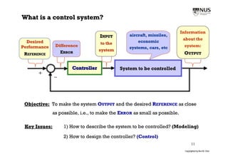
  • 1. What is a control system? Information INPUT aircraft, missiles, about the Desired to the economic Performance Difference systems, cars, etc system: ERROR system REFERENCE OUTPUT Controller System to be controlled + – Objective: To make the system OUTPUT and the desired REFERENCE as close as possible, i.e., to make the ERROR as small as possible. Key Issues: 1) How to describe the system to be controlled? (Modeling) 2) How to design the controller? (Control) 11 Copyrighted by Ben M. Chen
  • 2. Back to systems – block diagram representation of a system u(t) y(t) System u(t) is a signal or certain information injected into the system, which is called the system input, whereas y(t) is a signal or certain information produced by the system with respect to the input signal u(t). y(t) is called the system output. For example, R1 input: voltage source + output: voltage across R2 + u(t)  R2 y(t) ─ R2 y (t )   u (t ) R1  R2 16 Copyrighted by Ben M. Chen
  • 3. Linear systems u(t) y(t) System Let y1(t) be the output produced by an input signal u1(t) and y2(t) be the output produced by another input signal u2(t). Then, the system is said to be linear if a) the input is  u1(t), the output is  y1(t), where  is a scalar; and b) the input is u1(t) + u2(t), the output is y1(t) + y2(t). Or equivalently, the input is  u1(t) +  u2(t), the output is  y1(t) +  y2(t). Such a property is called superposition. For the circuit example on the previous page,   u1 (t )   u 2 (t )   R2 R2 R2 y (t )  u1 (t )   u 2 (t )   y1 (t )   y 2 (t ) R1  R2 R1  R2 R1  R2 It is a linear system! We will mainly focus on linear systems in this course. 17 Copyrighted by Ben M. Chen
  • 4. Example for nonlinear systems Example: Consider a system characterized by y (t )  100u 2 (t ) Step One: y1 (t )  100u12 (t ) & y 2 (t )  100  u 2 (t ) 2 Step Two: Let u (t )  u1 (t )  u 2 (t ), we have y (t )  100u 2 (t )  100[u1 (t )  u2 (t )]2  100[u12 (t )  u2 (t )  2u1 (t )u2 (t )] 2  y1 (t )  y2 (t )  200u1 (t )u2 (t )  y1 (t )  y2 (t ) The system is nonlinear. Exercise: Verify that the following system y (t )  cos(u (t )) is a nonlinear system. Give some examples in our daily life, which are nonlinear. 18 Copyrighted by Ben M. Chen
  • 5. Time invariant systems u(t) y(t) System A system is said to be time-invariant if for a shift input signal u( t t0), the output of the system is y( t t0). To see if a system is time-invariant or not, we test a) Find the output y1(t) that corresponds to the input u1(t). b) Let u2(t) = u1(tt0) and then find the corresponding output y2(t). c) If y2(t) = y1(tt0), then the system is time-invariant. Otherwise, it is not! In common words, if a system is time-invariant, then for the same input signal, the output produced by the system today will be exactly the same as that produced by the system tomorrow or any other time. 19 Copyrighted by Ben M. Chen
  • 6. Example for time invariant systems Consider the same circuit, i.e., R2 y (t )   u (t ) R1  R2 Obviously, whenever you apply a same voltage to the circuit, its output will always be the same. Let us verify this mathematically. Step One: R2 R2 y1 (t )   u1 (t )  y1 (t  t 0 )   u1 (t  t 0 ) R1  R2 R1  R2 Step Two: Let u 2 (t )  u1 (t  t 0 ), we have R2 R2 y 2 (t )   u 2 (t )   u1 (t  t 0 )  y1 (t  t 0 ) R1  R2 R1  R2 By definition, it is time-invariant! 20 Copyrighted by Ben M. Chen
  • 7. Example for time variant systems Example 1: Consider a system characterized by y (t )  cos(t )u (t ) Step One: y1 (t )  cos(t )  u1 (t )  y1 (t  t 0 )  cos(t  t 0 )  u1 (t  t 0 ) Step Two: Let u 2 (t )  u1 (t  t 0 ) , we have y 2 (t )  cos(t )  u 2 (t )  cos(t )  u1 (t  t 0 )  y1 (t  t 0 ) The system is not time-invariant. It is time-variant! Example 2: Consider a financial system such as a stock market. Assume that you invest $10,000 today in the market and make $2000. Is it guaranteed that you will make exactly another $2000 tomorrow if you invest the same amount of money? Is such a system time-invariant? You know the answer, don’t you? 21 Copyrighted by Ben M. Chen
  • 8. Systems with memory and without memory u(t) y(t) System A system is said to have memory if the value of y(t) at any particular time t1 depends on the time from   to t1. For example, + dy (t ) 1 t u(t) ~ C y(t) u (t )  C dt  y (t )  C  u(t )dt  ─ On the other hand, a system is said to have no memory if the value of y(t) at any particular time t1 depends only on the time t1. For example, R1 + R2 + y (t )   u (t ) u(t)  R2 y(t) R1  R2 ─ 22 Copyrighted by Ben M. Chen
  • 9. Causal systems u(t) y(t) System A causal system is a system where the output y(t) at a particular time t1 depends on the input for t  t1. For example, + dy (t ) 1 t u(t) ~ C y(t) u (t )  C dt  y (t )  C  u( )d  ─ On the other hand, a system is said to be non-causal if the value of y(t) at a particular time t1 depends on the input u(t) for some t > t1. For example, y (t )  u (t  1) in which the value of y(t) at t = 0 depends on the input at t = 1. 23 Copyrighted by Ben M. Chen
  • 10. System stability u(t) y(t) System The signal u(t) is said to be bounded if |u(t)| <  <  for all t, where  is real scalar. A system is said to be BIBO (bounded-input bounded-output) stable if its output y(t) produced by any bounded input is bounded. A BIBO stable system: y (t )  e u ( t )  | y (t ) |  e u ( t )  e   e    A BIBO unstable system: t t t y (t )   u( )d  Let u (t )  1, which is bounded. Then, y (t )   u( )d   d     24 Copyrighted by Ben M. Chen
  • 11. Linear differential equations General solution: n th order linear d n xt  d n 1 xt  differential equation  a n 1    a0 xt   u t  dt n dt n 1 General solution xt   x ss t   xtr t  Steady state response x ss t   particular integral obtained from assuming with no arbitrary solution to have the same form as u t  constant Transient response with xtr t   general solution of homogeneou s equation n arbitrary constants d n xtr t  d n 1 xtr t   a n 1    a0 xtr t   0 dt n dt n 1 33 Copyrighted by Ben M. Chen
  • 12. General solution of homogeneous equation: n th order linear d n xtr t  d n 1 xtr t  homogeneous equation n  a n 1 n 1    a0 xtr t   0 dt dt Roots of polynomial roots : z1 , ,z n from homogeneous equation given by z z1  z z n   z n  an 1 z n 1    a0 General solution xtr t   k1e z1t    k n e z n t (distinct roots) General solution   xtr t   k1  k 2 t  k 3t 2 e13t  k 4  k 5t  e 22t  k 6 e 31t  k 7 e 41t (non-distinct roots) if roots are 13, 13, 13, 22 , 22 , 31, 41 34 Copyrighted by Ben M. Chen
  • 13. Particular integral: x ss t  Any specific solution (with no arbitrary constant) of d n xt  d n 1 xt   an 1    a0 xt   u t  dt n dt n 1 Method to determine Trial and error approach: assume x ss t  to have x ss t  the same form as u t  and substitute into differential equation Example to find x ss t  for Try a solution of he 3t dxt  dx t  2 xt   e3t dt  2 x t   e 3t 3he 3t 2he 3t e 3t  h0.2 dt x ss t   0.2e 3t Standard trial solutions u t  trial solution for xss t  et het t ht tet h1h2t et a cos t   b sin  t  h1 cos t   h2 sin  t  35 Copyrighted by Ben M. Chen
  • 14. Time-domain System Models & Dynamic Responses 36 Copyrighted by Ben M. Chen
  • 15. RL circuit and governing differential equation Consider determining i(t) in the following series RL circuit: i (t) t=0 5 3V 7H v(t) where the switch is open for t < 0 and is closed for t  0. Since i(t) and v(t) will not be equal to constants or sinusoids for all time, these cannot be represented as constants or phasors. Instead, the basic general voltage-current relationships for the resistor and inductor have to be used: 37 Copyrighted by Ben M. Chen
  • 16. For t < 0 5 i (t) i (t) t =0 5 t<0 3 v(t) = 7 d i(t) 5 i (t) 7 dt i (t) = 0 5 3 7 d i(t) v(t) = 7 dt 3 5 i (t) = 0 i (t) = 0 voltage cross 5 over the switch d i(t) 3 KVL 7 v(t) = 7 =0 dt 38 Copyrighted by Ben M. Chen
  • 17. t 0 0 5 i (t) i (t) 5 3 7 d i (t) v(t) = 7 dt Applying KVL: Mathematically, the above d.e. is often written as di t  7  5 i t   3, t  0 di t   5 i t   u t , t  0 dt 7 dt and i(t) can be found from determining the general solution to this first order linear where the r.h.s. is u t   3, t  0 differential equation (d.e.) which governs and corresponds to the dc source or the behavior of the circuit for t  0. excitation in this example. 39 Copyrighted by Ben M. Chen
  • 18. Steady state response iss t   3 Since the r.h.s. of the governing d.e. , t 0 5 dit  7  5it   u t   3, t  0 dt Let us try a steady state solution of diss t  d 3 3 7 5iss t   7    5   3, t0 dt dt  5  5 iss t   k , t  0 and is a solution of the governing d.e. which has the same form as u(t), as a possible solution. In mathematics, the above solution is called the particular integral or solution di t  7 ss  5iss t   3 dt and is found from letting the answer to  70   5k   3 have the same form as u(t). The word 3 "particular" is used as the solution is only  k 5 one possible function that satisfy the d.e. 40 Copyrighted by Ben M. Chen
  • 19. In circuit analysis, the derivation of iss(t) by letting the answer to have the same form as u(t) can be shown to give the steady state response of the circuit as t  . t  i (t) = k Using KVL, the steady state 5 response is 3 7 d i(t) v(t) = 7 dt 3  0  5k  0  5k 3 k 5 i (t) = 5 k 5 3  it   , t   i (t) = k 5 5 3 d i(t) 7 v(t) = 7 =0 dt This is the same as iss(t). 41 Copyrighted by Ben M. Chen
  • 20. Transient response To determine i(t) for all t, it is necessary to find the complete solution of the governing d.e. di t  7  5i t   u t   3, t  0 dt From mathematics, the complete solution can be obtained from summing a particular solution, say, iss(t), with itr(t): i t   iss t   itr t , t  0 where itr(t) is the general solution of the homogeneous equation di t  5  t 7  5i t   0, t  0 i tr t   k 1 e z1 t  k1 e 7 , t0 dt di t  where k1 is a constant (unknown now). 7 tr  5itr t  dt ditr t  5 replaced by z  t dt itr t   k1e 7  0, t  7 z  5z  7 z  5 1 0 Thus, it is called transient response. 5 z1   42 7 Copyrighted by Ben M. Chen
  • 21. Complete response To see that summing iss(t) and itr(t) gives the general solution of the governing ODE di t  7  5i t   3, t  0 dt note that 3 d  3   5 3   3, i ss t   , t0 satisfies 7     t0 5 dt 5 5 5  t d  7t   7t  5 5 itr t   k1e 7 , t 0 satisfies 7  k1e   5 k1e   0, t  0 dt          t 5 3  t  5 3  t  5 i ss t   itr t   3  k 1 e 7 , t  0 satisfies 7 d   k1e 7   5  k1e 7   3 5 dt 5  5      5 3  t i t   iss t   itr t    k1e 7 , t  0 is the general solution of the ODE 5 43 Copyrighted by Ben M. Chen
  • 22. 3 5 i ss ( t ) 0 steady state response t <0 t 0 Switch close k1 5t i tr ( t ) = k 1e 7 , t0 k1 transient response e 0 t =0 t = 7 (Time constant) k1 is to be 5 determined later k1 + 3 5 i ss ( t ) + i tr ( t ) 3 complete response 5 0 44 Complete response Copyrighted by Ben M. Chen
  • 23. Note that the time it takes for the transient or zero-input response itr(t) to decay to 1/e of its initial value is 7 Time taken for itr(t) to decay to 1/e of initial value  5 and is called the time constant of the response or system. We can take the transient response to have died out after a few time constants. For the RC circuit, 100 At the time equal to 3 time 90 constants, the magnitude is about 5% of the peak. 80 70 Magnitude in Percentage At the time equal to 4 time 60 constants, the magnitude is 50 about 1.83% of the peak. 40 x 100/e 30 At the time equal to 5 time 20 constants, the magnitude is 10 about 0.68% of the peak 0 0 1 2 3 4 5 6 7 8 9 10 Time (second) 45 7/5 Copyrighted by Ben M. Chen
  • 24. A cruise control system  acceleration x A cruise-control x displacement system friction force b x mass force u m By the well-known Newton’s Law of motion: f = m a, where f is the total force applied to an object with a mass m and a is the acceleration, we have b u u  bx  m  x    x x  m m This a 2nd order Ordinary Differential Equation with respect to displacement x. It can  be written as a 1st order ODE with respect to speed v = x : b u v  v  model of the cruise control system, u is input force, v is output. m m 60 Copyrighted by Ben M. Chen
  • 25. Assume a passenger car weights 1 ton, i.e., m = 1000 kg, and the friction coefficient of a certain situation b = 100 N·s/m. Assume that the input force generated by the car engine is u = 1000 N and the car is initially parked, i.e., x(0) = 0 and v(0) = 0. Find the solutions for the car velocity v(t) and displacement x(t). For the velocity model, model b u v  v  v  0.1v  1  m m The steady state response: It is obvious that vss = 10 m/s = 36 km/h The transient response: Characteristic polynomial z + 0.1 = 0, which gives z1 = 0.1. 10 0.1t 0.1t vtr (t )  k1e  v(t )  vss  vtr (t )  10  k1e 8 v(0) = 0 implies that k1 = 10 and hence Velocity (m/s) 6 4  0.1t v(t )  vss  vtr (t )  10  10e 2 61 What is the time constant for this system? 0 0 20 40 60 80 100 Time (second)
  • 26. For the dynamic model in terms of displacement, u  bx  m  x    0.1x  1 x  The steady state response: From the solution for the velocity, which is a constant, we can conclude that the steady state solution for the displacement is xss = vsst = 10t. The transient response: Characteristic polynomial z2 + 0.1z = 0, which gives z1 = 0.1 and z2 = 0. The transient solution is then given by xtr (t )  k1e 0.1t  k 2 e 0t  k1e 0.1t  k 2 and hence the complete solution x(t )  xss  xtr (t )  10t  k1e 0.1t  k 2  v(t )  x(t )  10  0.1k1e 0.1t  x(0) = 0 implies k1 + k2 = 0 and v(0) = 0 implies 10  0.1 k1 = 0. Thus, k1 = 100, k2 =  100. x(t )  10t  100e 0.1t  100 62 Copyrighted by Ben M. Chen
  • 27. Complete response for the car displacement 800 700 600 500 Displacement (m) 400 300 200 100 0 0 10 20 30 40 50 60 70 80 Time (second) Exercise: Show that the car cruise control system is BIBO stable for its velocity model and it BIBO unstable for its displacement model. 63 Copyrighted by Ben M. Chen
  • 28. Behaviors of a general 2nd order system Consider a general 2nd order system (an RLC circuit or a mechanical system or whatever) governed by an ODE a(t )  by (t )  cy (t )  u (t ) y  Its transient response (or natural response) is fully characterized the properties of its homogeneous equation or its characteristic polynomial, i.e., a(t )  by (t )  cy (t )  0  az 2  bz  c  0 y  The latter has two roots at two real distinct roots if b2  4ac > 0  b  b 2  4ac z1, 2  = two complex conjugate roots if b2  4ac < 0 2a two identical roots if b2  4ac = 0 These different types of roots give different natures of responses. 64 Copyrighted by Ben M. Chen
  • 29. Overdamped systems Overdamped response is referred to the situation when the characteristic polynomial has two distinct negative real roots, i.e., ab > 0 & b2  4ac > 0. For example, (t )  6 y (t )  5 y (t )  0 y  which has a characteristic polynomial, z 2  6 z  5  0  z1, 2  1,  5  y (t )  k1e t  k 2 e 5t , y (t )  k1e t  5k 2 e 5t  Assume that y (0)  0, y (0)  4 , which implies  1 0.8 y (0)  k1  k 2  0 0.6 k1  1, k 2  1 0.4 y (0)   k1  5k 2  4  0.2 Magnitude 0 and thus, -0.2 y (t )  e t  e 5t -0.4 -0.6 -0.8 What is the dominating time constant? -1 65 0 1 2 3 4 5 6 7 8 9 10 Time (second)
  • 30. Underdamped systems Underdamped response is referred to the situation when the characteristic polynomial has two complex conjugated roots negative real part, i.e., ab > 0 & b2  4ac < 0. For example, (t )  2 y (t )  101 y (t )  0 y  which has a characteristic polynomial, z 2  2 z  101  0  z1, 2  1  j10  y (t )  k1e ( 1 j10 )t  k 2 e ( 1 j10 )t  e t (k1e j10t  k 2 e  j10t ) y (t )  e t [k1 (cos10t  j sin 10t )  k 2 (cos10t  j sin 10t )]  e t [(k1  k 2 ) cos10t  j (k1  k 2 ) sin 10t ] Assume that y (0)  0, y (0)  10 , which implies  y (0)  k1  k 2  0 j (k 1k 2 )  1  y (t )  e t sin 10t y (0)  (k1  k 2 )  j10(k 1k 2 )  10  The time constant for such a system is determined by the exponential term. 66 Copyrighted by Ben M. Chen
  • 31. Underdamped response et 1 0.8 0.6 0.4 0.2 Magnitude 0 -0.2 -0.4 -0.6 -0.8 -1 0 1 2 3 4 5 6 7  et Time (second) 67 Copyrighted by Ben M. Chen
  • 32. Critically damped systems Critically damped response is corresponding to the situation when the characteristic polynomial has two identical negative real roots, i.e., ab > 0 & b2  4ac = 0. For example, (t )  2 y (t )  y (t )  0 y  which has a characteristic polynomial, z 2  2 z  1  0  z1, 2  1  y (t )  k1e  t  k 2te t  e t (k1  k 2t ) y (t )  e t (k 2  k1  k 2t )  Assume that y (0)  1, y (0)  1 , which implies  1.4 1.2 y (0)  k1  1 k1  1, k 2  2 1 y (0)  k 2  k1  1  0.8 Magnitude 0.6 and thus 0.4 y (t )  e t (1  2t ) 0.2 68 0 0 2 4 6 8 10 Time (second)
  • 33. Never damped (unstable) systems Never damped response is corresponding to the situation when the characteristic polynomial has at least one root with a nonnegative real part. For example, (t )  y (t )  0 y which has a characteristic polynomial, z 2  1  0  z1, 2  1  y (t )  k1e  t  k 2 et  y (t )   k1e  t  k 2 et  Assume that y (0)  2, y (0)  0 , which implies  450 400 y (0)  k1  k 2  2 k1  k 2  1 350 y (0)  k 2  k1  0  300 Magnitude 250 and thus 200 y (t )  e t  et 150 100 50 It is an unstable system. We’ll study more on it. 0 69 0 1 2 3 4 5 6 Time (second)
  • 34. Review of Laplace Transforms 70 Copyrighted by Ben M. Chen
  • 35. Introduction Let us first examine the following time-domain functions: 1 2 1.5 0.5 1 0.5 Magnitude Magnitude 0 0 -0.5 -0.5 -1 -1.5 -1 -2 0 1 2 3 4 5 6 7 8 9 10 0 1 2 3 4 5 6 7 8 9 10 Time in Seconds Time in Seconds A cosine function with a frequency f = 0.2 Hz. x (t )  cos0.4t   sin 0.8t  cos1.6t  Note that it has a period T = 5 seconds. What are frequencies of this function? Laplace transform is a tool to convert time-domain functions into a frequency-domain ones in which information about frequencies of the function can be captured. It is often much easier to solve problems in frequency-domain with the help of Laplace transform. 71 Copyrighted by Ben M. Chen
  • 36. Laplace Transform Given a time-domain function f (t), the one-sided Laplace transform is defined as follows:  F ( s )  L f (t )   f (t )e  st dt , s    j 0 where the lower limit of integration is set to 0 to include the origin (t = 0) and to capture any discontinuities of the function at t = 0. The integration for the Laplace transform might not convert to a finite solution for arbitrary time-domain function. In order for the integration to convert to a final value, which implies that the Laplace transform for the given function is existent, we need     (  j ) t t  jt | F ( s ) |   f (t )e dt   f (t )  e e dt   f (t )  e  t dt   0 0 0 for some real scalar  = c . Clearly, the integration exists for all   c, which is called the region of convergence (ROC). Laplace transform is undefined outside of ROC. 72 Copyrighted by Ben M. Chen
  • 37. Example 1: Find the Laplace transform of a unit step function f(t) = 1(t) = 1, t  0.    1 1  1  1  1  1 F ( s )  1(t )e  st dt   e  st dt   e  st   e      e 0     0     1  0 0 s 0 s  s  s  s  s Clearly, the about result is valid for s =  + j with  > 0. Example 2: Find the Laplace transform of an exponential function f (t) = e – a t, t  0.     1  s  a t 1 F ( s)   f (t )e  st dt   e at e  st dt   e  s  a t dt   e  0 0 0 sa 0 sa Again, the result is only valid for all s =  + j with  >  a. imag axis imag axis real axis real axis 0 a ROC for Example 1 ROC for Example 2 73 Copyrighted by Ben M. Chen
  • 38. Example 3: Find the Laplace transform of a unit impulse function  (t), which has the following properties: 1.  (t) = 0 for t  0 2.  (0)     3.   (t )dt  1,  f (t ) (t )dt  f (0) for any f (t)   4.  (t) is an even function, i.e.,  (t) =  (t) Its Laplace transform is significant to many system and control problems. By definition,  L (t )    (t )e  st dt  e 0  1 0 Its ROC is the whole complex plane. Obviously, impulse functions are non-existent in real life. We will learn from a tutorial question on how to approximate such a function. 74 Copyrighted by Ben M. Chen
  • 39. Inverse Laplace Transform Given a frequency-domain function F(s), the inverse Laplace transform is to convert it back to its original time-domain function f (t). ROC  1  j f (t )  L1 F ( s )  1  F ( s )e ds st 1 2 j  1  j This process is quite complex because it requires knowledge about complex analysis. We use look-up table rather than evaluating these complex integrals. The functions f(t) and F(s) are one-to-one pairing each other and are called Laplace transform pair. Symbolically, f (t )  F ( s ) 75 Copyrighted by Ben M. Chen
  • 40. Properties of Laplace transform: 1. Superposition or linearity: La1 f1 (t )  a2 f 2 (t )  a1L f1 (t ) a2 L f 2 (t )  a1F1 ( s )  a2 F2 ( s ) Example: Find the Laplace transform of cos(t). By Euler’s formula, we have cos(t )  2  1 j t e  e  j t  By the superposition property, we have 1    1    Lcos(t )  L  e jt  e  jt   L e jt  e  jt 1  2  2 2 1  1   1  1 s  j  s  j s        2 2  s  j   s  j  2 ( s  j )s  j  s   2     76 Copyrighted by Ben M. Chen
  • 41. 2. Scaling: If F(s) is the Laplace transform of f(t), then 1 s L f ( at )  F  a a Example: It was shown in the previous example that Lcos(t )  s s2   2 By the scaling property, we have s  s  1  Lcos(2t )  1 2 2 s   2  2 2 s 2 2s  4 2  s  4 2  2   4  4  which may also be obtained by replacing  by 2. 77 Copyrighted by Ben M. Chen
  • 42. 3. Time shift (delay): f(t) If F(s) is the Laplace transform of f(t), then f(t  a) L f (t  a )  1(t  a)  e  as F ( s ) a For a function delayed by ‘a’ in time-domain, the equivalence in s-domain is multiplying its original Laplace transform of the function by eas. Example: Lcos t   s s  Lcos( (t  a ))  1(t  a )  e  as s2   2 s2   2 78 Copyrighted by Ben M. Chen
  • 43. 4. Frequency shift: If F(s) is the Laplace transform of f(t), then Example: Given cos(t )  s  and sin(t )  s2   2 s2   2 Using the shift property, we obtain the Laplace transforms of the damped sine and cosine functions as    L e  at cos(t )  sa ( s  a) 2   2 and   L e  at sin(t )  ( s  a) 2   2 79 Copyrighted by Ben M. Chen
  • 44. 5. Differentiation:   Lf (t )  sL f (t )  f (0 )  sF ( s )  f (0 )  df (t )     L  dt   d 2 f (t )    L(t )  s L f (t )  sf (0 )  f (0 )  s F ( s )  sf (0 )  f (0 ) 2   2   L 2 f  dt  6. Integration: t  1 L   f  d   L f (t )  F ( s ) 1 0  s s Example: The derivative of a unit step function 1(t) is a unit impulse function (t). d 1(t )   (t ) dt d  1 t  1 L (t )  L  1(t )  sL (t )  1(0  )  s  0  1 1 1 L (t )  L     d   L (t )  1  dt  s 0   s s 80 Copyrighted by Ben M. Chen
  • 45. 7. Periodic functions: If f (t) is a periodic function, then it can be represented as the sum of time-shifted functions as follows: f (t )  f1 (t )  f 2 (t )  f 3 (t )    f1 (t )  f1 (t  T )  f1 (t  2T )   Applying time-shift property, we obtain F ( s )  F1 ( s )  F1 ( s )e  sT  F1 ( s )e  s 2T  T  st F1 ( s )  f (t )e dt 0  F1 ( s )(1  e  sT  e  s 2T )   sT  1 e 1  e  sT 81 Copyrighted by Ben M. Chen
  • 46. 8. Initial value theorem: Examining the differentiation property of the Laplace transform, i.e.,   Lf (t )  sL f (t )  f (0 )  sF ( s )  f (0 )  df (t )     L  dt  we have   df (t )   df (t )  st  sF ( s )  f (0 )  L    e dt   e  st df (t )  0, as s    dt  0  dt 0 Thus, f (0  )  sF ( s ), as s   or f (0  )  lim [ sF ( s )] s  This is called the initial value theorem of Laplace transform. For example, recall that sa f (t )  e  at cos(t )  F (s)  ( s  a) 2   2 s( s  a) s 2  as f (0)  e cos(0)  1 0  lim [ sF ( s )]  lim  lim 2 1 s  ( s  a )   s   s  2 as  ( a   ) 2 2 2 2 s  82 Copyrighted by Ben M. Chen
  • 47. 9. Final value theorem: Examining again the differentiation property of the Laplace transform, i.e.,   Lf (t )  sL f (t )  f (0 )  sF ( s )  f (0 )  df (t )     L  dt  we have     df (t )  df (t )  st df (t ) 0t  lim [ sF ( s )  f (0 )]  lim L    lim  e dt   e dt  f (t ) 0   f ()  f (0  ) s 0 s  0  dt  s  0 0  dt 0  dt Thus, The result is only valid for a function whose f ()  lim [ sF ( s )] F(s) has all its poles in the open left-half s 0 plane (a simple pole at s = 0 permitted)! This is called the final value theorem of Laplace transform. For example, sa f (t )  e  at cos(t )  F (s)  ( s  a) 2   2  s( s  a) s 2  as f ( )  e cos()  0  lim [ sF ( s )]  lim  lim 2 0 s 0 ( s  a )   s  0 s  2 as  ( a   ) 2 2 2 2 s 0 83 Copyrighted by Ben M. Chen
  • 48. Summary of Laplace transform properties Property f (t) F (s) Linearity Scaling Time shift Frequency shift Time derivative t Time integration  f  d 0 F1 ( s ) Time periodicity 1  e  sT Initial value f (0  ) Final value Convolution 84 Courtesy of Dr Melissa Tao
  • 49. Some commonly used Laplace transform pairs f (t )  F ( s) f (t )  F ( s)  (t )  1  sin t  s2   2 1 1(t )  s s cos t  s2   2 1 s sin    cos t  sin(t   )  s2 s2   2 tn  n! s cos    sin  cos(t   )  s n 1 s2   2 1  e  at  e  at sin t  sa s  a 2   2 te  at  1 sa e  at cos t  s  a 2 s  a 2   2 85 Copyrighted by Ben M. Chen
  • 50. Why Laplace transform? Allows us to work with algebraic equations rather than differential equations. Provides an easy way to solve system Applicable to a Laplace transform is problems involving wider variety of significant for many initial conditions. inputs than phasor reasons analysis Capable of giving us the total response (natural and forced) of the circuit in one single operation. 86 Courtesy of Dr Melissa Tao
  • 51. Frequency-domain Descriptions of Linear Systems 87 Copyrighted by Ben M. Chen
  • 52. Frequency domain model of linear systems – transfer functions A linear system expressed in terms of an ODE is called a model in the time domain. In what follows, we will learn that the same system can be expressed in terms of a rational function of s, the Laplace transform variable. Recall the cruise control system u  bx  m  x  m  bx  u x  Assume that the initial conditions are zero. Taking Laplace transform on its both sides, (ms 2  bs) X ( s )  ms 2 X ( s )  bsX ( s )  Lm  bx  Lu  U ( s ) x  we obtain a rational function of s, i.e., X (s) 1 1 H (s)   2 X ( s )  H ( s )U ( s )  U (s) U ( s ) ms  bs ms  bs 2 H(s) is the ratio of the system output (displacement) and input (force) in frequency domain. Such a function is called the transfer function of the system, which fully characterizes the system properties. 96 Copyrighted by Ben M. Chen
  • 53. More example: the series RLC circuit The ODE for the general series RLC circuit was derived earlier as the following: d 2 vC t  dv t  LC  RC C  vC t   v(t ) dt 2 dt Assume that all initial conditions are zero (note that for deriving transfer functions, we always assume initial conditions are zero!).  d 2 vC t  dvC t   ( LCs  RCs  1)VC ( s )  L  LC 2  RC  vC t   Lv(t )  V ( s )  dt 2 dt  VC ( s ) 1 1 H (s)   VC ( s )  H ( s )V ( s )  V ( s) V ( s ) LCs 2  RCs  1 LCs  RCs  1 2 H(s) is the ratio of the system output (capacitor voltage) and input (voltage source) in frequency domain. The circuit (or the system) is fully characterized by the transfer function. If the H(s) and V(s) are known, we can compute the system output. As such, it is important to study the properties of H(s)! 97 Copyrighted by Ben M. Chen
  • 54. System poles and zeros As we have seen from the previous examples, a general linear time-invariant system can be expressed in a frequency-domain model or transfer function: U(s) Y(s) H(s) with N ( s ) bm s m  bm 1s m 1    b1s  b0 H (s)   n n 1 , mn D( s) s  an 1s    a1s  a0 n is called the order of the system. The roots of the numerator of H(s), i.e., N(s), are called the system zeros (because the transfer function is equal to 0 at these points), and the roots of the denominator of H(s), i.e., D(s), are called the system poles (the transfer function is singular at these points). It turns out that the system properties are fully captured by the locations of these poles and zeros… 98 Copyrighted by Ben M. Chen
  • 55. Examples: 1 1 m The cruise control system has a transfer function H ( s )  2  ms  bs s ( s  b ) m It has no zero at all and two poles at s  0, s   b m 1 The RLC circuit has a transfer function H ( s )  LCs 2  RCs  1 It has no zero and two poles at  RC  ( RC ) 2  4 LC  RC  ( RC ) 2  4 LC s1  , s2  2 LC 2 LC which are precisely the same as the roots of the characteristic polynomial of its ODE. 5s 2  10 s  5 5( s  1) 2 The system H ( s )  3  has two zeros (repeated) s  6 s  11s  6 ( s  1)( s  2)( s  3) 2 at s = 1 and three poles at s  1, s  2, s  3 , respectively. 99 Copyrighted by Ben M. Chen
  • 56. Response to sinusoidal inputs Let us consider the series RL circuit whose current governed by the following ODE di t  I (s) 0 .2 5  5 i t   v t   ( 5 s  5) I ( s )  V ( s )  H (s)   dt V (s) s  1 Let the voltage source be a sinusoidal v(t) = cos (2t), which has a Laplace transform s 0 .2 0.2 s A Bs  C V (s)   I ( s)  V (s)   2   2 s 4 2 s 1 s 1 s  4 s 1 s  4 Using the coefficient matching method, we have to match ( A  B ) s 2  ( B  C ) s  ( 4 A  C )  0 .2 s 0.04 s  0.16 0.04 0.04 s 0.08  2 0.04 I (s)      s2  4 s  1 s 2  22 s 2  22 s  1  A B  0  A  0.04     B  C  0.2   B  0.04 4 A  C  0  C  0.16  i (t )  0.04[cos(2t )  2 sin( 2t )  e t ] The steady state response is the given by iss (t )  0.04[cos(2t )  2 sin(2t )]  0.0894 cos(2t  63.4349 ). 100 Copyrighted by Ben M. Chen
  • 57. Let us solve the problem using another approach. Noting that v(t) = cos (2t), which has an angular frequency of  = 2 rad/sec, and noting that the transfer function I (s) 0 .2 H (s)   V (s) s  1 is nothing more than the ratio or gain between the system input and output in the frequency domain. Let us calculate the ‘gain’ of H(s) at the particular frequency coinciding with the input signal, i.e., at s = j with  = 2. 0 .2 0 .2 H ( j 2 )  H ( j )   2    0.0894 e  j1.1071  0.0894   63 .4349  j  1   2 j 2  1 It simply means that at  = 2 rad/sec, the input signal is amplified by 0.0894 and its phase is shifted by  63.4349 degrees. It is obvious then the system output, i.e., the current in the circuit at the steady state is given by iss (t )  0.0894 cos(2t  63.4349 ). which is identical to what we have obtained earlier. Actually, by letting s = j, the above approach is the same as the phasor technique for AC circuits. 101 Copyrighted by Ben M. Chen
  • 58. Frequency response – amplitude and phase responses It can be seen from the previous example that for an AC circuits or for a system with a sinusoidal input, the system steady state output can be easily evaluated once the amplitude and phase of its transfer function are known. Thus, it is useful to ‘compute’ the amplitude and phase of the transfer function, i.e., H ( j  )  H ( s ) s  j  H ( j  )   H ( j  ) It is obvious that both magnitude and phase of H(j) are functions of . The plot of |H(j)| is called the magnitude (amplitude) response of H(j) and the plot of H(j) is called the phase response of H(j). Together they are called the frequency response of the transfer function. In particularly, |H(0)| is called the DC gain of the system (DC is equivalent to k cos(t) with  = 0). The frequency response of a circuit or a system is an important concept in system theory. It can be used to characterize the properties of the circuit or system, and used to evaluated the system output response. 102 Copyrighted by Ben M. Chen
  • 59. Example: Let us reconsider the series RL circuit with the following transfer function: I (s) 0 .2 0 .2 0 .2 H (s)    H ( j )   H ( j )   H ( j )    tan 1  V (s) s  1 j  1 1 2 Thus, it is straightforward, but very tedious, to compute its amplitude and phase.   0.01  H ( j )  0.2, H ( j )  0.57  0.2 0.15   0.1  H ( j )  0.199,  H ( j )  5.71 Magnitude 0.1   0.2  H ( j )  0.196,  H ( j )  11.31 0.05   0.5  H ( j )  0.179,  H ( j )  26.57  0 -2 -1 0 1 2 3  1  H ( j )  0.141,  H ( j )  45 10 10 10 10 10 10 Frequency (rad/sec) 0 2  H ( j )  0.089,  H ( j )  63.43  5  H ( j )  0.039,  H ( j )  78.69 Phase (degrees) -50   10  H ( j )  0.020,  H ( j )  84.29   100  H ( j )  0.002,  H ( j )  89.43 -100 -2 -1 0 1 2 3 10 10 10 10 10 10   1000  H ( j )  0.0002,  H ( j )  89.94 Frequency (rad/sec) 103 Copyrighted by Ben M. Chen
  • 60. Note that in the plots of the magnitude and phase responses, we use a log scale for the frequency axis. If we draw in a normal scale, the responses will look awful. There is another way to draw the frequency response. i.e., directly draw both magnitude and phase on a complex plane, which is called the polar plot. For the example considered, its polar plot is given as follows: 0.1 0.2 0.08 0.15 Magnitude 0.06 0.1 0.04 0.05 0.02 0 imag axis -2 -1 0 1 2 3 10 10 10 10 10 10 0 Frequency (rad/sec) 0 -0.02 -20 Phase (degrees) -0.04 -40 -0.06 -60 -0.08 -80 -0.1 -100 -0.2 -0.15 -0.1 -0.05 0 0.05 0.1 0.15 0.2 10 -2 -1 10 10 0 10 1 10 2 10 3 read axis Frequency (rad/sec) The red-line curves are more accurate plots using MATLAB. 104 Copyrighted by Ben M. Chen
  • 61. What can we observe from the frequency response? 0.2 0.15 Magnitude 0.1 0.05 0 -2 -1 0 1 2 3 10 10 10 10 10 10 Frequency (rad/sec) 0 -20 Phase (degrees) -40 -60 -80 -100 -2 -1 0 1 2 3 10 10 10 10 10 10 Frequency (rad/sec) At low frequencies, magnitude At low frequencies, magnitude For large frequencies, the magnitude For large frequencies, the magnitude response is relatively aalarge. response is relatively large. response is small and thus signals response is small and thus signals Thus, the corresponding output Thus, the corresponding output with large frequencies is attenuated with large frequencies is attenuated will be large. will be large. or blocked. or blocked. 105 Copyrighted by Ben M. Chen
  • 62. Lowpass systems 0.2 1 0.8 0.15 0.6 0.1 0.4 0.05 0.2 -0.2 0 Lowpass System 0 -0.05 -0.4 -0.1 -0.6   0.1 rad/sec -0.15 -0.8 -1 -0.2 0 10 20 30 40 50 60 70 80 90 100 0 10 20 30 40 50 60 70 80 90 100 Time (second) Time (second) 0.04 1 0.8 0.03 0.6 0.02 0.4 0.2 0.01 0 -0.2 Lowpass System 0 -0.4 -0.01 -0.6 -0.8   10 rad/sec -0.02 0 1 2 3 4 5 6 7 8 9 10 -1 0 1 2 3 4 5 6 7 8 9 10 Time (second) Time (second) 106 Copyrighted by Ben M. Chen
  • 63. Bode plot The plots of the magnitude and phase responses of a transfer function are called the Bode plot. The easiest way to draw Bode plot is to use MATLAB (i.e., bode function). However, there are some tricks that can help us to sketch Bode plots (approximation) without computing detailed values. To do this, we need to introduce a scale called dB (decibel). Given a positive scalar a, its decibel is defined as 20  log 10 ( a ) . For example, a 1  20  log 10 ( a )  0  a  0 dB a  10  20  log 10 ( a )  20  a  20 dB a  100  20  log 10 ( a )  40  a  40 dB a    20  log 10 (   )  20  log 10 ( )  20  log 10 (  )  a   in dB   in dB a  20  log 10 (    )  20  log 10 ( )  20  log 10 (  )  a   in dB   in dB In the dB scale, the product of two scalars becomes an addition and the division of two scalars becomes a subtraction. 107 Copyrighted by Ben M. Chen
  • 64. Bode plot – an integrator We start with finding the Bode plot asymptotes for a simple system characterized by 1 1 1 H (s)   H ( j )   H ( j )  H ( j )    90  s j  Examining the amplitude in dB scale, i.e., 1 20  log 10 H ( j )  20  log 10  20  log 10  dB  it is simple to see that   1  20  log 10 H ( j1)  20  log 10 1  0 dB   10  20  log 10 H ( j10 )  20  log 10 10  20 dB    2  101  20  log 10 H ( j 2 )  20  log 10  2  20  log 10 101  20  log 10 10  20  log 10 1  20  20  log 10 1 dB Thus, the above expressions clearly indicate that the magnitude is reduced by  20 dB when the frequency is increased by 10 times. It is equivalent to say that the magnitude times 108 is rolling off 20 dB per decade. Copyrighted by Ben M. Chen
  • 65. The phase response of an integrator is  90 degrees, a constant. The Bode plot of an integrator is given by Bode Diagram 20 rolling off 0 20 dB per Magnitude (dB) -20 decade -40 -60 -89 -89.5 constant Phase (deg) -90 phase -90.5 response -91 -1 0 1 2 3 10 10 10 10 10 Frequency (rad/sec) 109 Copyrighted by Ben M. Chen