SlideShare a Scribd company logo
1 of 7
Download to read offline
Using RES2DMOD and RES2DINV to Explore Electrical Resistivity Results
This is an introduction to resistivity software followed by a few exercises with four objectives:
1. get a feel for working with electrical resistivity data
2. learn what psuedosections look like for known models
3. experiment with noise and removing noisy observations, and
4. compare Wenner and dipole-dipole arrays.
The two programs, RES2DMOD and RES2DINV, are from http://www.geoelectrical.com/. The
modeling program is available on the web site as is a demo version of the inversion program. For both
programs, the manuals are detailed and good as are the help documents available from the menu bar; this
is a short, ‘quick start’, synopsis. The site also has an excellent tutorial on electrical methods.
RES2DMOD
For RES2DMOD, the general sequence is to open a file, calculate the results, and display the model and
results. From there, you can change array types, edit the model, change resistivities, or save the model
for RES2DINV. There are a number of canned models that install with the program.
From the menu bar in RES2DMOD (bullets indicate individual steps)
• FILE – read file with forward model. Now, the example files should show up. If they don’t they
are in the installation directory. Choose Blocks_up.mod
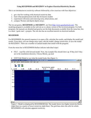
• EDIT/Edit Model to see what the model looks like (figure 1).
Figure 1. Model as displayed by RES2DMOD/Edit. The model shows two higher resistivity blocks
(light blue) in a matrix of lower resistivity (dark blue). The grid lines show the cells for which
RES2DMOD will calculate apparent resistivity.
• MODEL COMPUTATION – calculate the apparent resistivity values.
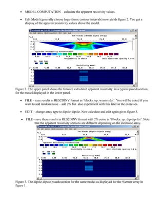
• Edit Model (generally choose logarithmic contour intervals) now yields figure 2. You get a
display of the apparent resistivity values above the model.
Figure 2. The upper panel shows the forward calculated apparent resistivity, in a typical psuedosection,
for the model displayed in the lower panel.
• FILE – save results in RES2DINV format as ‘blocks_up_wenner.dat’. You will be asked if you
want to add random noise – add 2% but also experiment with this later in the exercises.
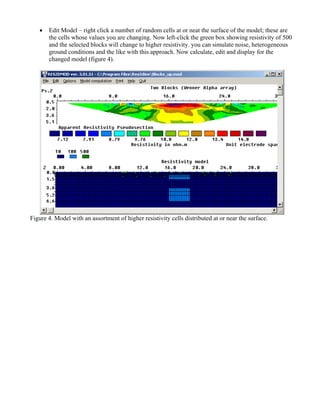
• EDIT – change array type to dipole-dipole. Now calculate and edit again gives figure 3.
• FILE - save these results in RES2DINV format with 2% noise in ‘Blocks_up_dip-dip.dat’. Note
that the apparent resistivity sections are different depending on the electrode array.
Figure 3. The dipole-dipole psuedosection for the same model as displayed for the Wenner array in
figure 1.
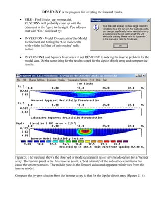
• Edit Model – right click a number of random cells at or neat the surface of the model; these are
the cells whose values you are changing. Now left-click the green box showing resistivity of 500
and the selected blocks will change to higher resistivity. you can simulate noise, heterogeneous
ground conditions and the like with this approach. Now calculate, edit and display for the
changed model (figure 4).
Figure 4. Model with an assortment of higher resistivity cells distributed at or near the surface.
RES2DINV is the program for inverting the forward results.
• FILE – Find Blocks_up_wenner.dat.
RES2DINV will probably come up with the
comment in the figure to the right. You address
that with ‘OK’, followed by:
• INVERSION - Model Discretization/Use Model
Refinement and hitting the ‘Use model cells
with widths half that of unit spacing’ radio
button.
• INVERSION/Least Squares Inversion will set RES2DINV to solving the inverse problem for the
model data. Do the same thing for the results stored for the dipole-dipole array and compare the
results.
Figure 5. The top panel shows the observed or modeled apparent resistivity pseudosection for a Wenner
array. The bottom panel is the final inverse result, a 'best estimate' of the subsurface conditions that
cause the observed results. The middle panel is the forward calculated apparent resistivities from the
inverse model.
Compare the inverse solution from the Wenner array to that for the dipole-dipole array (figures 5, 6).
Figure 6. The top panel shows the observed or modeled apparent resistivity pseudosection for a
dipole-dipole array. The bottom panel is the final inverse result, a 'best estimate' of the
subsurface conditions that cause the observed results. The middle panel is the forward calculated
apparent resistivities from the inverse model.
Experimenting with heterogeneous conditions. Inverting the data where some extra high
resistivity blocks were added yield a somewhat different result (figure 7).
Figure 7. Inverse solution for the data for which included a distribution of high resistivity cells
near the surface.
Editing Data using EDIT/exterminate bad datum points. RES2DINV allows you to remove results
from the observed pseudosection via a display such as figure 8. The prime question you always need to
ask before such a procedure is: how do you know the points are “bad”? You can use this feature as a
way to guide your understanding of results and to suggest further experiments.
Figure 8. RES2DINV’s display for “exterminating bad datum points”.
In Figure 8, the points in red, which were selected with mouse clicking, are to be eliminated from the
subsequent inversion. Once you exit the “edit Data Window”, save the altered data set with a new name
(e.g., modified.dat). You can use this editing feature to test the impact on, or a few, apparent resistivities
has on the solution. Other features will help your visualization and understanding:
Inversion/Model Discretization/Display Model Blocks:
Inversion/Model Sensitivity Options/Display Model Blocks Sensitivity

More Related Content

What's hot

Lecture 13-electrical method -field procedure
Lecture 13-electrical method -field procedureLecture 13-electrical method -field procedure
Lecture 13-electrical method -field procedure
Kosygin Leishangthem
 

What's hot (20)

Lecture 13-electrical method -field procedure
Lecture 13-electrical method -field procedureLecture 13-electrical method -field procedure
Lecture 13-electrical method -field procedure
 
Dual laterolog
Dual laterologDual laterolog
Dual laterolog
 
Exploration Geophysics III semester.pdf
Exploration Geophysics III semester.pdfExploration Geophysics III semester.pdf
Exploration Geophysics III semester.pdf
 
Rock Physics: Slides
Rock Physics: SlidesRock Physics: Slides
Rock Physics: Slides
 
Geophysical methods brief summary
Geophysical methods brief summaryGeophysical methods brief summary
Geophysical methods brief summary
 
Resistivity method
Resistivity method Resistivity method
Resistivity method
 
Applications Gravity survey Magnetic survey Electrical resistivity survey Sei...
Applications Gravity survey Magnetic survey Electrical resistivity survey Sei...Applications Gravity survey Magnetic survey Electrical resistivity survey Sei...
Applications Gravity survey Magnetic survey Electrical resistivity survey Sei...
 
Seismic Attributes .pptx
Seismic Attributes .pptxSeismic Attributes .pptx
Seismic Attributes .pptx
 
Electrical survey 2018
Electrical survey 2018Electrical survey 2018
Electrical survey 2018
 
Rock Mass Classification
Rock Mass ClassificationRock Mass Classification
Rock Mass Classification
 
Well logging
Well loggingWell logging
Well logging
 
Introduction to Seismic Method
Introduction to Seismic Method Introduction to Seismic Method
Introduction to Seismic Method
 
Resistivity log
Resistivity logResistivity log
Resistivity log
 
Basics of seismic interpretation
Basics of seismic interpretationBasics of seismic interpretation
Basics of seismic interpretation
 
Session 1 log-analysis
Session 1 log-analysisSession 1 log-analysis
Session 1 log-analysis
 
2 D 3D_ seismic survey
2 D 3D_ seismic survey2 D 3D_ seismic survey
2 D 3D_ seismic survey
 
Electrical method
Electrical methodElectrical method
Electrical method
 
SP Log
SP Log SP Log
SP Log
 
geophysical exploration
geophysical explorationgeophysical exploration
geophysical exploration
 
Geomechanics
Geomechanics Geomechanics
Geomechanics
 

Similar to Modeling electrical resistivity with res2 dmod

ECE321322 Electronics I & Lab Spring 2015 1 Final P.docx
ECE321322 Electronics I & Lab Spring 2015 1 Final P.docxECE321322 Electronics I & Lab Spring 2015 1 Final P.docx
ECE321322 Electronics I & Lab Spring 2015 1 Final P.docx
jack60216
 
Problem 7PurposeBreak apart a complicated system.ConstantsC7C13.docx
Problem 7PurposeBreak apart a complicated system.ConstantsC7C13.docxProblem 7PurposeBreak apart a complicated system.ConstantsC7C13.docx
Problem 7PurposeBreak apart a complicated system.ConstantsC7C13.docx
LacieKlineeb
 
MultiLevelROM_ANS_Summer2015_RevMarch23
MultiLevelROM_ANS_Summer2015_RevMarch23MultiLevelROM_ANS_Summer2015_RevMarch23
MultiLevelROM_ANS_Summer2015_RevMarch23
Mohammad Abdo
 
EELE 5331 Digital ASIC DesignLab ManualDr. Yushi Zhou.docx
EELE 5331 Digital ASIC DesignLab ManualDr. Yushi Zhou.docxEELE 5331 Digital ASIC DesignLab ManualDr. Yushi Zhou.docx
EELE 5331 Digital ASIC DesignLab ManualDr. Yushi Zhou.docx
toltonkendal
 
1.9 GHz Low Noise Amplifier
1.9 GHz Low Noise Amplifier1.9 GHz Low Noise Amplifier
1.9 GHz Low Noise Amplifier
Xavier Edokpa
 
32 bit×32 bit multiprecision razor based dynamic
32 bit×32 bit multiprecision razor based dynamic32 bit×32 bit multiprecision razor based dynamic
32 bit×32 bit multiprecision razor based dynamic
Mastan Masthan
 
Design ofexperimentstutorial
Design ofexperimentstutorialDesign ofexperimentstutorial
Design ofexperimentstutorial
Ingrid McKenzie
 

Similar to Modeling electrical resistivity with res2 dmod (20)

Steady state CFD analysis of C-D nozzle
Steady state CFD analysis of C-D nozzle Steady state CFD analysis of C-D nozzle
Steady state CFD analysis of C-D nozzle
 
Magazine awr-ims-3
Magazine awr-ims-3Magazine awr-ims-3
Magazine awr-ims-3
 
Excel solver
Excel solverExcel solver
Excel solver
 
ECE321322 Electronics I & Lab Spring 2015 1 Final P.docx
ECE321322 Electronics I & Lab Spring 2015 1 Final P.docxECE321322 Electronics I & Lab Spring 2015 1 Final P.docx
ECE321322 Electronics I & Lab Spring 2015 1 Final P.docx
 
IPI2win 2..pdf
IPI2win 2..pdfIPI2win 2..pdf
IPI2win 2..pdf
 
Tutorial solar module(physical-model)
Tutorial solar module(physical-model)Tutorial solar module(physical-model)
Tutorial solar module(physical-model)
 
Ads
AdsAds
Ads
 
3 2 dobos - whats new in sam - pv modeling workshop may 2016
3 2 dobos - whats new in sam - pv modeling workshop may 20163 2 dobos - whats new in sam - pv modeling workshop may 2016
3 2 dobos - whats new in sam - pv modeling workshop may 2016
 
Solar cell Modeling with Scaps 1-D
Solar cell Modeling with Scaps 1-D Solar cell Modeling with Scaps 1-D
Solar cell Modeling with Scaps 1-D
 
Problem 7PurposeBreak apart a complicated system.ConstantsC7C13.docx
Problem 7PurposeBreak apart a complicated system.ConstantsC7C13.docxProblem 7PurposeBreak apart a complicated system.ConstantsC7C13.docx
Problem 7PurposeBreak apart a complicated system.ConstantsC7C13.docx
 
Article jd2
Article jd2Article jd2
Article jd2
 
Cadence manual
Cadence manualCadence manual
Cadence manual
 
MultiLevelROM_ANS_Summer2015_RevMarch23
MultiLevelROM_ANS_Summer2015_RevMarch23MultiLevelROM_ANS_Summer2015_RevMarch23
MultiLevelROM_ANS_Summer2015_RevMarch23
 
Development of Multi-level Reduced Order MOdeling Methodology
Development of Multi-level Reduced Order MOdeling MethodologyDevelopment of Multi-level Reduced Order MOdeling Methodology
Development of Multi-level Reduced Order MOdeling Methodology
 
EELE 5331 Digital ASIC DesignLab ManualDr. Yushi Zhou.docx
EELE 5331 Digital ASIC DesignLab ManualDr. Yushi Zhou.docxEELE 5331 Digital ASIC DesignLab ManualDr. Yushi Zhou.docx
EELE 5331 Digital ASIC DesignLab ManualDr. Yushi Zhou.docx
 
1.9 GHz Low Noise Amplifier
1.9 GHz Low Noise Amplifier1.9 GHz Low Noise Amplifier
1.9 GHz Low Noise Amplifier
 
MSPWM Based Implementation of Novel 5-level Inverter with Photovoltaic System
MSPWM Based Implementation of Novel 5-level Inverter with Photovoltaic SystemMSPWM Based Implementation of Novel 5-level Inverter with Photovoltaic System
MSPWM Based Implementation of Novel 5-level Inverter with Photovoltaic System
 
How To Diffuse
How To DiffuseHow To Diffuse
How To Diffuse
 
32 bit×32 bit multiprecision razor based dynamic
32 bit×32 bit multiprecision razor based dynamic32 bit×32 bit multiprecision razor based dynamic
32 bit×32 bit multiprecision razor based dynamic
 
Design ofexperimentstutorial
Design ofexperimentstutorialDesign ofexperimentstutorial
Design ofexperimentstutorial
 

Recently uploaded

Module for Grade 9 for Asynchronous/Distance learning
Module for Grade 9 for Asynchronous/Distance learningModule for Grade 9 for Asynchronous/Distance learning
Module for Grade 9 for Asynchronous/Distance learning
levieagacer
 
Conjugation, transduction and transformation
Conjugation, transduction and transformationConjugation, transduction and transformation
Conjugation, transduction and transformation
Areesha Ahmad
 
Asymmetry in the atmosphere of the ultra-hot Jupiter WASP-76 b
Asymmetry in the atmosphere of the ultra-hot Jupiter WASP-76 bAsymmetry in the atmosphere of the ultra-hot Jupiter WASP-76 b
Asymmetry in the atmosphere of the ultra-hot Jupiter WASP-76 b
Sérgio Sacani
 
Bacterial Identification and Classifications
Bacterial Identification and ClassificationsBacterial Identification and Classifications
Bacterial Identification and Classifications
Areesha Ahmad
 
Biogenic Sulfur Gases as Biosignatures on Temperate Sub-Neptune Waterworlds
Biogenic Sulfur Gases as Biosignatures on Temperate Sub-Neptune WaterworldsBiogenic Sulfur Gases as Biosignatures on Temperate Sub-Neptune Waterworlds
Biogenic Sulfur Gases as Biosignatures on Temperate Sub-Neptune Waterworlds
Sérgio Sacani
 

Recently uploaded (20)

GBSN - Microbiology (Unit 2)
GBSN - Microbiology (Unit 2)GBSN - Microbiology (Unit 2)
GBSN - Microbiology (Unit 2)
 
Module for Grade 9 for Asynchronous/Distance learning
Module for Grade 9 for Asynchronous/Distance learningModule for Grade 9 for Asynchronous/Distance learning
Module for Grade 9 for Asynchronous/Distance learning
 
Locating and isolating a gene, FISH, GISH, Chromosome walking and jumping, te...
Locating and isolating a gene, FISH, GISH, Chromosome walking and jumping, te...Locating and isolating a gene, FISH, GISH, Chromosome walking and jumping, te...
Locating and isolating a gene, FISH, GISH, Chromosome walking and jumping, te...
 
Kochi ❤CALL GIRL 84099*07087 ❤CALL GIRLS IN Kochi ESCORT SERVICE❤CALL GIRL
Kochi ❤CALL GIRL 84099*07087 ❤CALL GIRLS IN Kochi ESCORT SERVICE❤CALL GIRLKochi ❤CALL GIRL 84099*07087 ❤CALL GIRLS IN Kochi ESCORT SERVICE❤CALL GIRL
Kochi ❤CALL GIRL 84099*07087 ❤CALL GIRLS IN Kochi ESCORT SERVICE❤CALL GIRL
 
Clean In Place(CIP).pptx .
Clean In Place(CIP).pptx                 .Clean In Place(CIP).pptx                 .
Clean In Place(CIP).pptx .
 
module for grade 9 for distance learning
module for grade 9 for distance learningmodule for grade 9 for distance learning
module for grade 9 for distance learning
 
Conjugation, transduction and transformation
Conjugation, transduction and transformationConjugation, transduction and transformation
Conjugation, transduction and transformation
 
pumpkin fruit fly, water melon fruit fly, cucumber fruit fly
pumpkin fruit fly, water melon fruit fly, cucumber fruit flypumpkin fruit fly, water melon fruit fly, cucumber fruit fly
pumpkin fruit fly, water melon fruit fly, cucumber fruit fly
 
9654467111 Call Girls In Raj Nagar Delhi Short 1500 Night 6000
9654467111 Call Girls In Raj Nagar Delhi Short 1500 Night 60009654467111 Call Girls In Raj Nagar Delhi Short 1500 Night 6000
9654467111 Call Girls In Raj Nagar Delhi Short 1500 Night 6000
 
Proteomics: types, protein profiling steps etc.
Proteomics: types, protein profiling steps etc.Proteomics: types, protein profiling steps etc.
Proteomics: types, protein profiling steps etc.
 
Factory Acceptance Test( FAT).pptx .
Factory Acceptance Test( FAT).pptx       .Factory Acceptance Test( FAT).pptx       .
Factory Acceptance Test( FAT).pptx .
 
Asymmetry in the atmosphere of the ultra-hot Jupiter WASP-76 b
Asymmetry in the atmosphere of the ultra-hot Jupiter WASP-76 bAsymmetry in the atmosphere of the ultra-hot Jupiter WASP-76 b
Asymmetry in the atmosphere of the ultra-hot Jupiter WASP-76 b
 
Forensic Biology & Its biological significance.pdf
Forensic Biology & Its biological significance.pdfForensic Biology & Its biological significance.pdf
Forensic Biology & Its biological significance.pdf
 
Call Girls Ahmedabad +917728919243 call me Independent Escort Service
Call Girls Ahmedabad +917728919243 call me Independent Escort ServiceCall Girls Ahmedabad +917728919243 call me Independent Escort Service
Call Girls Ahmedabad +917728919243 call me Independent Escort Service
 
Bacterial Identification and Classifications
Bacterial Identification and ClassificationsBacterial Identification and Classifications
Bacterial Identification and Classifications
 
300003-World Science Day For Peace And Development.pptx
300003-World Science Day For Peace And Development.pptx300003-World Science Day For Peace And Development.pptx
300003-World Science Day For Peace And Development.pptx
 
Justdial Call Girls In Indirapuram, Ghaziabad, 8800357707 Escorts Service
Justdial Call Girls In Indirapuram, Ghaziabad, 8800357707 Escorts ServiceJustdial Call Girls In Indirapuram, Ghaziabad, 8800357707 Escorts Service
Justdial Call Girls In Indirapuram, Ghaziabad, 8800357707 Escorts Service
 
Pulmonary drug delivery system M.pharm -2nd sem P'ceutics
Pulmonary drug delivery system M.pharm -2nd sem P'ceuticsPulmonary drug delivery system M.pharm -2nd sem P'ceutics
Pulmonary drug delivery system M.pharm -2nd sem P'ceutics
 
Biogenic Sulfur Gases as Biosignatures on Temperate Sub-Neptune Waterworlds
Biogenic Sulfur Gases as Biosignatures on Temperate Sub-Neptune WaterworldsBiogenic Sulfur Gases as Biosignatures on Temperate Sub-Neptune Waterworlds
Biogenic Sulfur Gases as Biosignatures on Temperate Sub-Neptune Waterworlds
 
Thyroid Physiology_Dr.E. Muralinath_ Associate Professor
Thyroid Physiology_Dr.E. Muralinath_ Associate ProfessorThyroid Physiology_Dr.E. Muralinath_ Associate Professor
Thyroid Physiology_Dr.E. Muralinath_ Associate Professor
 

Modeling electrical resistivity with res2 dmod

  • 1. Using RES2DMOD and RES2DINV to Explore Electrical Resistivity Results This is an introduction to resistivity software followed by a few exercises with four objectives: 1. get a feel for working with electrical resistivity data 2. learn what psuedosections look like for known models 3. experiment with noise and removing noisy observations, and 4. compare Wenner and dipole-dipole arrays. The two programs, RES2DMOD and RES2DINV, are from http://www.geoelectrical.com/. The modeling program is available on the web site as is a demo version of the inversion program. For both programs, the manuals are detailed and good as are the help documents available from the menu bar; this is a short, ‘quick start’, synopsis. The site also has an excellent tutorial on electrical methods. RES2DMOD For RES2DMOD, the general sequence is to open a file, calculate the results, and display the model and results. From there, you can change array types, edit the model, change resistivities, or save the model for RES2DINV. There are a number of canned models that install with the program. From the menu bar in RES2DMOD (bullets indicate individual steps) • FILE – read file with forward model. Now, the example files should show up. If they don’t they are in the installation directory. Choose Blocks_up.mod • EDIT/Edit Model to see what the model looks like (figure 1). Figure 1. Model as displayed by RES2DMOD/Edit. The model shows two higher resistivity blocks (light blue) in a matrix of lower resistivity (dark blue). The grid lines show the cells for which RES2DMOD will calculate apparent resistivity.
  • 2. • MODEL COMPUTATION – calculate the apparent resistivity values. • Edit Model (generally choose logarithmic contour intervals) now yields figure 2. You get a display of the apparent resistivity values above the model. Figure 2. The upper panel shows the forward calculated apparent resistivity, in a typical psuedosection, for the model displayed in the lower panel. • FILE – save results in RES2DINV format as ‘blocks_up_wenner.dat’. You will be asked if you want to add random noise – add 2% but also experiment with this later in the exercises. • EDIT – change array type to dipole-dipole. Now calculate and edit again gives figure 3. • FILE - save these results in RES2DINV format with 2% noise in ‘Blocks_up_dip-dip.dat’. Note that the apparent resistivity sections are different depending on the electrode array. Figure 3. The dipole-dipole psuedosection for the same model as displayed for the Wenner array in figure 1.
  • 3. • Edit Model – right click a number of random cells at or neat the surface of the model; these are the cells whose values you are changing. Now left-click the green box showing resistivity of 500 and the selected blocks will change to higher resistivity. you can simulate noise, heterogeneous ground conditions and the like with this approach. Now calculate, edit and display for the changed model (figure 4). Figure 4. Model with an assortment of higher resistivity cells distributed at or near the surface.
  • 4. RES2DINV is the program for inverting the forward results. • FILE – Find Blocks_up_wenner.dat. RES2DINV will probably come up with the comment in the figure to the right. You address that with ‘OK’, followed by: • INVERSION - Model Discretization/Use Model Refinement and hitting the ‘Use model cells with widths half that of unit spacing’ radio button. • INVERSION/Least Squares Inversion will set RES2DINV to solving the inverse problem for the model data. Do the same thing for the results stored for the dipole-dipole array and compare the results. Figure 5. The top panel shows the observed or modeled apparent resistivity pseudosection for a Wenner array. The bottom panel is the final inverse result, a 'best estimate' of the subsurface conditions that cause the observed results. The middle panel is the forward calculated apparent resistivities from the inverse model. Compare the inverse solution from the Wenner array to that for the dipole-dipole array (figures 5, 6).
  • 5. Figure 6. The top panel shows the observed or modeled apparent resistivity pseudosection for a dipole-dipole array. The bottom panel is the final inverse result, a 'best estimate' of the subsurface conditions that cause the observed results. The middle panel is the forward calculated apparent resistivities from the inverse model. Experimenting with heterogeneous conditions. Inverting the data where some extra high resistivity blocks were added yield a somewhat different result (figure 7). Figure 7. Inverse solution for the data for which included a distribution of high resistivity cells near the surface.
  • 6. Editing Data using EDIT/exterminate bad datum points. RES2DINV allows you to remove results from the observed pseudosection via a display such as figure 8. The prime question you always need to ask before such a procedure is: how do you know the points are “bad”? You can use this feature as a way to guide your understanding of results and to suggest further experiments. Figure 8. RES2DINV’s display for “exterminating bad datum points”. In Figure 8, the points in red, which were selected with mouse clicking, are to be eliminated from the subsequent inversion. Once you exit the “edit Data Window”, save the altered data set with a new name (e.g., modified.dat). You can use this editing feature to test the impact on, or a few, apparent resistivities has on the solution. Other features will help your visualization and understanding: Inversion/Model Discretization/Display Model Blocks: