Downloaded 146 times


![2.7
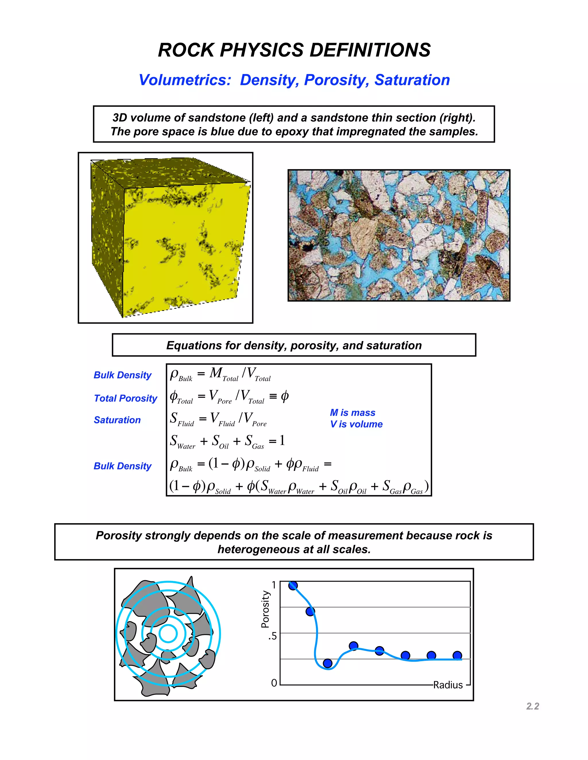
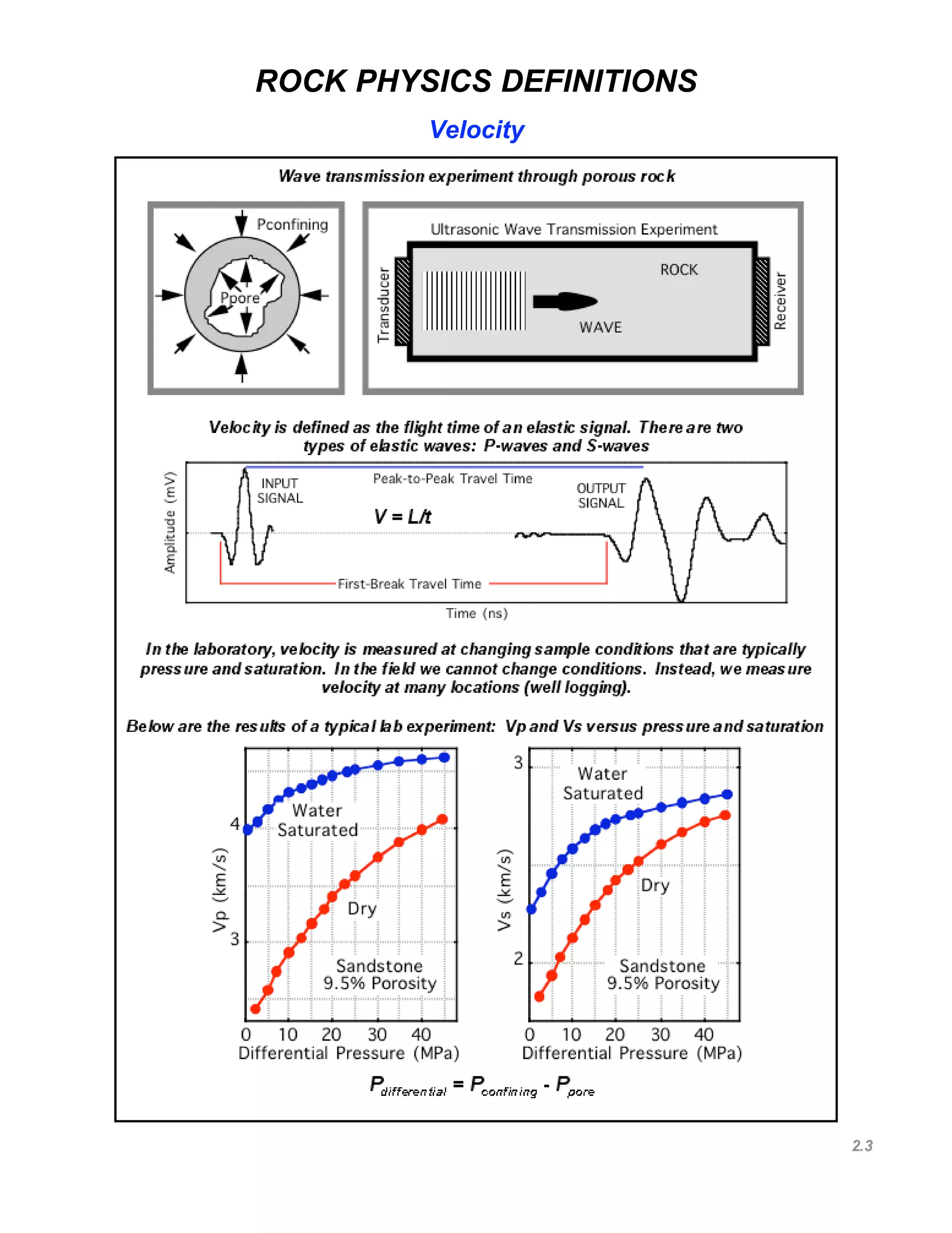
ROCK PHYSICS BASICS
Relative Impedance Inversion
€
Rpp (θ) ≈ Rpp (0) cos2
θ + 2.25Δν sin2
θ
≈ Rpp (0) + [2.25Δν − Rpp (0)]sin2
θ,
€
Rpp
(0) =
Ip 2
− Ip1
Ip 2
+ Ip1
=
dIp
2Ip
=
1
2
d ln Ip
,
€
Ip
= exp[2 Rpp
(0)dz∫ ].
€
Δν =
Rpp (θ )− Rpp(0) cos2
θ
2.25sin2
θ
,
ν =
Rpp
(θ )− Rpp
(0) cos2
θ
2.25sin2
θ
∫ dz.](https://image.slidesharecdn.com/rockphysicsdefinitions-151228092717/75/Rock-Physics-Definitions-7-2048.jpg)

![2.9
ROCK PHYSICS BASICS
Elasticity
Ti = σijnj
Stress Tensor
u
x1
x2
x3
x1
T
n
x2
x3
Strain Tensor
εij =
1
2
(
∂ui
∂x j
+
∂uj
∂xi
)
σij = σji i ≠ j; εij = εji i ≠ j.
σij = cijklekl; cijkl = cjikl = cijlk = cjilk, cijkl = cklij .
σij = λδijεαα + 2µεij; εij = [(1 + ν)σij − νδijσαα ]/ E.
Commonly used constants are: λ and µ -- Lame's constants; ν -- Poisson's ratio; E -- Young's modulus. The elastic
moduli are determined by the experiment performed. For example, the bulk modulus is measured in the
hydrostatic compression experiment. The shear modulus is measured in the shear deformation experiment.
Stress and strain. Forces acting within a mechanical body are mathematically
characterized by the stress tensor which is a 3x3 matrix. By using a stress tensor we
can find the vector of traction acting on an elemental plane of any orientation within
the body (figure on the left).
The deformation within the body is characterized by the strain tensor. This tensor is
formed by the derivatives of the components of the displacement of a material point in
the body (figure on the right).
Both stress and strain tensors are symmetrical matrices.
Hooke’s law relates stress to strain. It postulates that this relation is linear. In general, there are 21 independent
elastic constants that linearly relate stress to strain.
Fortunately, if a body is isotropic, only two independent elastic constants are required. These constants are
called elastic moduli.
Elastic moduli derived from loading experiments are called static moduli
Bulk Modulus
K = λ + 2µ / 3
Z
X
Y
σ xz = 2µε xz
εxx = εyy = εzz = εxy = 0
Shear
Shear Modulus Compressional Modulus
Hydrostatic Loading Distortion, no volume
change
No lateral deformation
€
M = K + (4 /3)µ](https://image.slidesharecdn.com/rockphysicsdefinitions-151228092717/75/Rock-Physics-Definitions-9-2048.jpg)


![2.16
ROCK PHYSICS BASICS
Elastic Composites and Elastic Bounds
Most physical bodies in nature are elastically heterogeneous, I.e., they are made of
components that have different elastic moduli. The effective elastic moduli of a
composite depend on (a) properties of individual components and (b) geometrical
arrangement of these components in space.
It is often very hard, if not impossible, to theoretically calculate the effective elastic
moduli of a composite.
However, elastic bounds help us contain the exact values of the effective elastic
moduli.
The simplest bounds are the Voigt (stiffest) and Reuss (softest) bound. No matter how
complex the composite is, its effective elastic moduli are contained within these
bounds.
Composite Voigt
Reuss
For an elastic modulus that may be either bulk or shear modulus of an N-component
composite where the i-th component has modulus Mi and occupies volume fraction
fi, the Voigt (upper) bound is:
MV = fi Mi
i =1
N
∑
MR = ( fi Mi
−1
i=1
N
∑ )−1
The Reuss (lower) bound is:
Hill’s average is simply the average between the Voigt and Reuss bounds:
MH =
MV + MR
2
=
1
2
[ fi Mi
i=1
N
∑ + ( fi Mi
−1
i=1
N
∑ )
−1
]
10
12
14
16
18
20
0 0.2 0.4 0.6 0.8 1
ElasticModulus
Volume Concentration
The graph on the right shows the Voigt and
Reuss bounds and Hill’s average of a two-
component composite.
The elastic modulus of the soft component is 10
and that of the stiff component is 20. The
horizontal axis is the concentration of the stiff
component.
Voigt
Reuss
Hill](https://image.slidesharecdn.com/rockphysicsdefinitions-151228092717/75/Rock-Physics-Definitions-16-2048.jpg)
![2.17
ROCK PHYSICS BASICS
Hashin-Shrikman Elastic Bounds
For an isotropic composite, the effective elastic bulk and shear moduli are
contained within rigorous Hashin-Shtrikman bounds. These bounds have been
derived for the bulk and shear moduli. The Hashin-Shtrikman bounds are tighter
than the Voigt-Reuss bounds.
[
fi
Ki + 4
3
Gmini =1
N
∑ ]−1
−
4
3
Gmin ≤ Keff ≤ [
fi
Ki + 4
3
Gmax
]−1
i =1
N
∑ −
4
3
Gmax,
[
fi
Gi +
Gmin
6
9Kmin + 8Gmin
Kmin + 2Gmin
]
−1
i =1
N
∑ −
Gmin
6
9Kmin + 8Gmin
Kmin + 2Gmin
≤ Geff ≤
[
fi
Gi +
Gmax
6
9Kmax + 8Gmax
Kmax + 2Gmax
i =1
N
∑ ]
−1
−
Gmax
6
9Kmax +8Gmax
Kmax + 2Gmax
,
In the Hashin-Shtrikman equations, the subscript “eff” is for the effective elastic
bulk and shear moduli. The subscripts “min” and “max” are for the softest and
stiffest components, respectively.
A physical realization of the Hashin-Shtrikman bounds for two components is the
entire space filled by composite spheres of varying size. The outer shell of each
sphere is the softest component for the lower bound and the stiffest component for
the upper bound.
If one of the components is void (empty pore) the lower bound is zero.
Hashin-Shtrikman
Bounds: Realization
10
12
14
16
18
20
0 0.2 0.4 0.6 0.8 1
ElasticModulus
Volume Concentration
Voigt
Reuss
Hashin-
Shtrikman](https://image.slidesharecdn.com/rockphysicsdefinitions-151228092717/75/Rock-Physics-Definitions-17-2048.jpg)


![2.25
ROCK PHYSICS BASICS
Stress-Induced Anisotropy
θ
€
Vp (θ) ≈ α(1+ δsin2
θcos2
θ + εsin4
θ)
VsV (θ) ≈ β[1+
α2
β2
(ε −δ)sin2
θcos2
θ]
VsH (θ) ≈ β[1+ γ sin2
θ]
€
ε =
Vp (π /2) −Vp (0)
Vp (0)
γ =
VsH (π /2) −VsV (π /2)
VsV (π /2)
=
VsH (π /2) −VsH (0)
VsH (0)
Thomsen's anisotropic formulation (weak transverse isotropy)
Vzz
Vyy
Vxx Vyz
VyxVxz
Vxy
Vzy
Vzx
Z
Y
X
Vzz
Vxx
Vyy
Vyz
Vyx
Vxz
Vzy
Vxy
Vzx
Ottawa sand. Uniaxial compression.
Pxx = Pyy = 1.72 bar. Yin (1992).
Anisotropic stress field induces anisotropy in otherwise isotropic rock.](https://image.slidesharecdn.com/rockphysicsdefinitions-151228092717/75/Rock-Physics-Definitions-25-2048.jpg)


![2.29
€
U1
€
U2
€
I
€
U = U1
−U2
R = U /I
Potential
Drop
Electrical
Current
Resistance
€
ρ = RA/l
Resistivity
€
[R] = Ω ≡ Ohm
[ρ] = Ω⋅ m ≡ Ohm⋅ m
€
σ =1/ρ
Conductivity
DEFINITIONS OF RESISTIVITY
0.1
1
10
100
6000 6500 7000 7500 8000
Rt(Ohmm)
Depth (ft)
0
50
100
150
6000 6500 7000 7500 8000
GR
Depth (ft)](https://image.slidesharecdn.com/rockphysicsdefinitions-151228092717/75/Rock-Physics-Definitions-29-2048.jpg)

1. The document defines key rock physics terms including density, porosity, saturation, velocity, impedance, Poisson's ratio, and reflection coefficients. Equations are provided for calculating these values from measured properties. 2. Methods of modeling reflection seismograms are described including normal reflection, reflection at an angle using Zoeppritz equations, AVO analysis, and impedance inversion. 3. Concepts of stress, strain, elasticity, elastic moduli, and their relationships to velocity are covered. The differences between static and dynamic moduli are also discussed.


