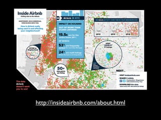
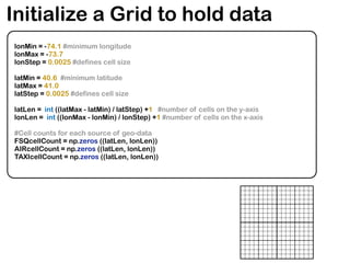
This document summarizes an analysis of geo-referenced data from location-based services and the sharing economy. It loads and analyzes data on venues and check-ins from Foursquare in New York City to generate a place network, examines the network's degree distributions and clustering, and identifies central places and nodes. It also loads taxi trip and Airbnb listing data and plots journeys and locations on a map. Finally, it discusses accessing Uber's API to query pricing data and the potential for combining different data sources to predict surge areas.
![Mining Geo-referenced Data: Location-based
Services and the Sharing Economy [Part 2]
Anastasios Noulas
Data Science Institute, Lancaster University
November 2015
PyData, NYC, 2015](https://image.slidesharecdn.com/pydataslidesmininggeoreferneddatanoulas-151110021020-lva1-app6892/85/Mining-Geo-referenced-Data-Location-based-Services-and-the-Sharing-Economy-1-320.jpg)
![Mining Geo-referenced Data: Location-based
Services and the Sharing Economy [Part 2]
Anastasios Noulas
Data Science Institute, Lancaster University
November 2015
PyData, NYC, 2015](https://image.slidesharecdn.com/pydataslidesmininggeoreferneddatanoulas-151110021020-lva1-app6892/75/Mining-Geo-referenced-Data-Location-based-Services-and-the-Sharing-Economy-1-2048.jpg)


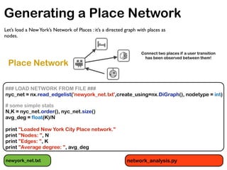
![Loading Foursquare places data
### READ FOURSQUARE VENUES DATA ###
node_data = {}
with open('venue_data_4sq_newyork_anon.csv') as csvfile:
reader = csv.DictReader(csvfile)
for row in reader:
latit = float(row['latitude'])
longit = float(row['longitude'])
place_title = row['title']
node_id = int(row['vid'])
node_data[node_id] = (place_title,latit,longit)
venue_data_4sq_newyork_anon.csv
network_analysis.py](https://image.slidesharecdn.com/pydataslidesmininggeoreferneddatanoulas-151110021020-lva1-app6892/85/Mining-Geo-referenced-Data-Location-based-Services-and-the-Sharing-Economy-7-320.jpg)
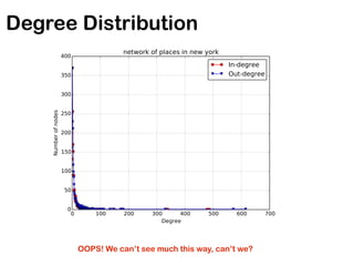
![Getting Degree Distributions
in_degrees = nyc_net.in_degree() #Get degree distributions (in- and out-)
in_values = sorted(set(in_degrees.values()))
in_hist = [in_degrees.values().count(x) for x in in_values]
out_degrees = nyc_net.out_degree()
out_values = sorted(set(out_degrees.values()))
out_hist = [out_degrees.values().count(x) for x in out_values]
# plot degree distributions
logScale = True #set this True to plot data in logarithmic scale
plt.figure()
if logScale:
plt.loglog(in_values,in_hist,'ro-') # red color with marker 'o'
plt.loglog(out_values,out_hist,'bv-') # blue color with marker 'v'
else:
plt.plot(in_values,in_hist,'ro-') # red color with marker 'o'
plt.plot(out_values,out_hist,'bv-') # blue color with marker 'v'
plt.legend(['In-degree','Out-degree'])
plt.xlabel('Degree')
plt.ylabel('Number of nodes')
plt.title('network of places in new york')
plt.grid(True)
if logScale:
plt.xlim([0,2*10**2])
plt.savefig('nyc_net_degree_distribution_loglog.pdf')
else:
plt.savefig('nyc_net_degree_distribution.pdf')
plt.close()](https://image.slidesharecdn.com/pydataslidesmininggeoreferneddatanoulas-151110021020-lva1-app6892/85/Mining-Geo-referenced-Data-Location-based-Services-and-the-Sharing-Economy-9-320.jpg)

![Triadic Formations in Networks
# Symmetrize the graph for simplcity
nyc_net_ud = nyc_net.to_undirected()
# We are interested in the largest connected component
nyc_net_components = nx.connected_component_subgraphs(nyc_net_ud)
nyc_net_mc = nyc_net_components[0]
# Graph statistics for the main component
N_mc, K_mc = nyc_net_mc.order(), nyc_net_mc.size()
avg_deg_mc = float(2*K_mc)/N_mc
avg_clust = nx.average_clustering(nyc_net_mc)
print ""
print "New York Place Network graph main component."
print "Nodes: ", N_mc
print "Edges: ", K_mc
print "Average degree: ", avg_deg_mc
print "Average clustering coefficient: ", avg_clust
We can get the clustering coefficient of individual nodes or of all the nodes
(but the first we convert the graph to an undirected one).](https://image.slidesharecdn.com/pydataslidesmininggeoreferneddatanoulas-151110021020-lva1-app6892/85/Mining-Geo-referenced-Data-Location-based-Services-and-the-Sharing-Economy-12-320.jpg)

![Most Central Nodes
def getTopDictionaryKeys(dictionary,number):
topList = []
a = dict(dictionary)
for i in range(0,number):
m = max(a, key=a.get)
topList.append([m,a[m]])
del a[m]
return topList
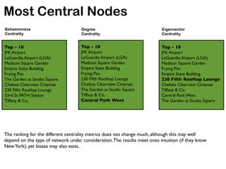
First we introduce a utility method: given a dictionary
and a threshold parameter, the top-K elements of the
dictionary are returned according to element values.
top_bet_cen = getTopDictionaryKeys(bet_cen,10)
top_deg_cen = getTopDictionaryKeys(deg_cen,10)
top_eig_cent = getTopDictionaryKeys(eig_cen,10)
We can then apply the method on the various centrality
methods available. Below we extract the top-10 most
central nodes for each case.](https://image.slidesharecdn.com/pydataslidesmininggeoreferneddatanoulas-151110021020-lva1-app6892/85/Mining-Geo-referenced-Data-Location-based-Services-and-the-Sharing-Economy-14-320.jpg)
![Interpretability Matters
print 'Top-10 places for betweenness centrality.'
for [node_id, value] in top_bet_cen:
title = node_data[node_id][0]
print title
print '------'
print 'Top-10 places for degree centrality.'
for [node_id, value] in top_deg_cen:
title = node_data[node_id][0]
print title
print '------'
print 'Top-10 places for eigenvector centrality.'
for [node_id, value] in top_eig_cent:
title = node_data[node_id][0]
print title
print '------'](https://image.slidesharecdn.com/pydataslidesmininggeoreferneddatanoulas-151110021020-lva1-app6892/85/Mining-Geo-referenced-Data-Location-based-Services-and-the-Sharing-Economy-15-320.jpg)
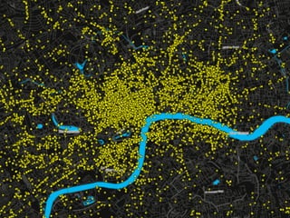
![# draw the graph using information about nodes geographic positions
pos_dict = {}
for node_id, node_info in node_data.items():
pos_dict[node_id] = (node_info[2], node_info[1])
nx.draw(nyc_net,pos=pos_dict,with_labels=False,node_size=20)
plt.savefig('nyc_net_graph.png')
plt.close()
Drawing the Graph](https://image.slidesharecdn.com/pydataslidesmininggeoreferneddatanoulas-151110021020-lva1-app6892/85/Mining-Geo-referenced-Data-Location-based-Services-and-the-Sharing-Economy-17-320.jpg)
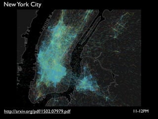


![Plotting taxi journey positions
import csv
from mpl_toolkits.basemap import Basemap
import matplotlib.pyplot as plt
#reading Taxi journey geographic coordinates #
taxi_coords = []
with open('taxi_trips.csv') as csvfile:
reader = csv.DictReader(csvfile)
for row in reader:
taxi_coords.append([float(row['latitude']), float(row['longitude'])])
y = [i[0] for i in taxi_coords]
x = [i[1] for i in taxi_coords]
colors = ['k' for i in range(0, len(y))]
popularities = [0.1 for i in range(0, len(y))]
m = Basemap(projection='merc',resolution='l',llcrnrlon=-74.0616,urcrnrlat=40.82,
urcrnrlon=-73.8563,llcrnrlat=40.699) #center map to NYC
# maps geocoordinates to pixel positions
x1,y1=m(x,y)
m.scatter(x1,y1,s=popularities,c=colors, marker="o",alpha=0.7)
plt.savefig('taxis.png')
plt.close()
taxi_trips.csv PlotTaxiPos.py](https://image.slidesharecdn.com/pydataslidesmininggeoreferneddatanoulas-151110021020-lva1-app6892/85/Mining-Geo-referenced-Data-Location-based-Services-and-the-Sharing-Economy-25-320.jpg)

![Loading Airbnb listings in NYC
id,listing_url,scrape_id,last_scraped,name,summary,space,description,experiences_offered,neighborhood_overview,notes,transit,thumbnail_url,medium_
url,picture_url,xl_picture_url,host_id,host_url,host_name,host_since,host_location,host_about,host_response_time,host_response_rate,
host_acceptance_rate,host_is_superhost,host_thumbnail_url,host_picture_url,host_neighbourhood,host_listings_count,host_total_listings_count,
host_verifications,host_has_profile_pic,host_identity_verified,street,neighbourhood,neighbourhood_cleansed,neighbourhood_group_cleansed,city,state,zipcode,
market,smart_location,country_code,country,latitude,longitude,is_location_exact,property_type,room_type,accommodates,bathrooms,
bedrooms,beds,bed_type,amenities,square_feet,price,weekly_price,monthly_price,security_deposit,cleaning_fee,guests_included,extra_people,minimum_nights
,maximum_nights,calendar_updated,has_availability,availability_30,availability_60,availability_90,availability_365,calendar_last_scraped,number_of_reviews,
first_review,last_review,review_scores_rating,review_scores_accuracy,review_scores_cleanliness,review_scores_checkin,review_scores_communication,review_
cores_location,review_scores_value,requires_license,license,jurisdiction_names,instant_bookable,cancellation_policy,require_guest_profile_picture,require_guest
_phone_verification,calculated_host_listings_count,reviews_per_month
A lot of fields in there: we pick only coordinates for this task!
airbnb_coords = []
with open('listings_sample.csv') as csvfile:
reader = csv.DictReader(csvfile)
for row in reader:
airbnb_coords.append([float(row['latitude']), float(row['longitude'])])
print 'Number of Airbnb listings: ' + str(len(airbnb_coords))
listings_sample.csv MultiLayerSurgePrediction.py](https://image.slidesharecdn.com/pydataslidesmininggeoreferneddatanoulas-151110021020-lva1-app6892/85/Mining-Geo-referenced-Data-Location-based-Services-and-the-Sharing-Economy-27-320.jpg)


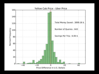
![(40.762211, -73.986389, {u'prices': [{u'localized_display_name': u'uberX', u'distance': 3.64,
u'display_name': u'uberX', u'product_id': u'b8e5c464-5de2-4539-a35a-986d6e58f186',
u'high_estimate': 23, u'surge_multiplier': 1.0, u'minimum': 8, u'low_estimate': 17, u'duration': 1205,
u'estimate': u'$17-23', u'currency_code': u'USD'}, {u'localized_display_name': u'uberXL', u'distance':
3.64, u'display_name': u'uberXL', u'product_id': u'1e0ce2df-4a1e-4333-86dd-dc0c67aaabe1',
u'high_estimate': 34, u'surge_multiplier': 1.0, u'minimum': 12, u'low_estimate': 25, u'duration': 1205,
u'estimate': u'$25-34', u'currency_code': u'USD'}, {u'localized_display_name': u'uberFAMILY',
u'distance': 3.64, u'display_name': u'uberFAMILY', u'product_id': u'd6d6d7ad-67f9-43ef-
a8de-86bd6224613a', u'high_estimate': 33, u'surge_multiplier': 1.0, u'minimum': 18, u'low_estimate':
27, u'duration': 1205, u'estimate': u'$27-33', u'currency_code': u'USD'}, {u'localized_display_name':
u'UberBLACK', u'distance': 3.64, u'display_name': u'UberBLACK', u'product_id': u'0e9d8dd3-
ffec-4c2b-9714-537e6174bb88', u'high_estimate': 40, u'surge_multiplier': 1.0, u'minimum': 15,
u'low_estimate': 31, u'duration': 1205, u'estimate': u'$31-40', u'currency_code': u'USD'},
{u'localized_display_name': u'UberSUV', u'distance': 3.64, u'display_name': u'UberSUV', u'product_id':
u'56487469-0d3d-4f19-b662-234b7576a562', u'high_estimate': 53, u'surge_multiplier': 1.0, u'minimum':
25, u'low_estimate': 43, u'duration': 1205, u'estimate': u'$43-53', u'currency_code': u'USD'},
{u'localized_display_name': u'uberT', u'distance': 3.64, u'display_name': u'uberT', u'product_id':
u'ebe413ab-cf49-465f-8564-a71119bfa449', u'high_estimate': None, u'surge_multiplier': 1.0,
u'minimum': None, u'low_estimate': None, u'duration': 1205, u'estimate': u'Metered', u'currency_code':
None}, {u'localized_display_name': u'Yellow WAV', u'distance': 3.64, u'display_name': u'Yellow WAV',
u'product_id': u'1864554f-7796-4043-82d4-883ddde1070a', u'high_estimate': 0, u'surge_multiplier':
1.0, u'minimum': 0, u'low_estimate': 0, u'duration': 1205, u'estimate': u'$0', u'currency_code': u'USD'}]},
40.757778, -73.94799)
Price Query output](https://image.slidesharecdn.com/pydataslidesmininggeoreferneddatanoulas-151110021020-lva1-app6892/85/Mining-Geo-referenced-Data-Location-based-Services-and-the-Sharing-Economy-31-320.jpg)
![Querying the Uber API (2)
f_out = open('UberQuestOutput.txt', 'w')
for i in range(0,1000):
coordsOrigin = random.choice(taxi_coords)
coordsDestination = random.choice(taxi_coords)
latitude_O = coordsOrigin[0]
longitude_O = coordsOrigin[1]
latitude_D = coordsDestination[0]
longitude_D = coordsDestination[1]
try:
uber_response = uber_request(latitude_O, longitude_O, 'price', latitude_D, longitude_D)
except:
time.sleep(10.0)
continue
print >> f_out, str((latitude_O, longitude_O, uber_response, latitude_D, longitude_D))
print 'Query retrieved, sleeping for a sec.'
time.sleep(1.0)
f_out.close()
print 'Uber Quest is Over.'
averageSurgeInCell.csv](https://image.slidesharecdn.com/pydataslidesmininggeoreferneddatanoulas-151110021020-lva1-app6892/85/Mining-Geo-referenced-Data-Location-based-Services-and-the-Sharing-Economy-32-320.jpg)
![Loading 3 geo-data layers
####### LOADING COORDS FROM 3 GEO LAYERS #########
airbnb_coords = []
with open('listings_sample.csv') as csvfile:
reader = csv.DictReader(csvfile)
for row in reader:
airbnb_coords.append([float(row['latitude']), float(row['longitude'])])
print 'Number of Airbnb listings: ' + str(len(airbnb_coords))
#reading Foursquare venue data #
foursquare_coords = []
with open('venue_data_4sq_newyork_anon.csv') as csvfile:
reader = csv.DictReader(csvfile)
for row in reader:
foursquare_coords.append([float(row['latitude']), float(row['longitude'])])
print 'Number of Foursquare listings: ' + str(len(foursquare_coords))
#reading Taxi journey coords #
taxi_coords = []
with open('taxi_trips.csv') as csvfile:
reader = csv.DictReader(csvfile)
for row in reader:
taxi_coords.append([float(row['latitude']), float(row['longitude'])])
print 'Number of Yellow Taxi journeys: ' + str(len(taxi_coords))](https://image.slidesharecdn.com/pydataslidesmininggeoreferneddatanoulas-151110021020-lva1-app6892/85/Mining-Geo-referenced-Data-Location-based-Services-and-the-Sharing-Economy-34-320.jpg)
![Count occurrences per cell
all_coords = [foursquare_coords, airbnb_coords, taxi_coords]
for i in range(0, 3):
current_coords = all_coords[i]
for coords in current_coords:
lat = coords[0]
longit = coords[1]
#if outside the grid then ingore point
if (lat < latMin) or (lat > latMax) or (longit < lonMin) or (longit > lonMax):
continue
#if outside the grid then ingore point
cx = int ((longit - lonMin) / lonStep)
cy = int((lat - latMin) / latStep)
if i == 0:
FSQcellCount[cy, cx] += 1
elif i == 1:
AIRcellCount[cy, cx] +=1
else:
TAXIcellCount[cy, cx] +=1](https://image.slidesharecdn.com/pydataslidesmininggeoreferneddatanoulas-151110021020-lva1-app6892/85/Mining-Geo-referenced-Data-Location-based-Services-and-the-Sharing-Economy-35-320.jpg)
![Loading and plotting average surge per area
#Load Area Average Surge: assume you have queried previously the UBER API and
have collected info on pricing for an area
latLongSurge = {}
for l in open('averageSurgeInCell.csv', 'r'):
splits = l.split(',')
cy = int(splits[0])
cx = int(splits[1])
averageSurgeCoeff = float(splits[2])
latLongSurge.setdefault(cy, {})
latLongSurge[cy][cx] = averageSurgeCoeff
###################
import pylab as plt
surgeValues = [latLongSurge[cy][cx] for cy in range(0, latLen-1) for cx in range(0,lonLen-1) if
latLongSurge[cy][cx] !=0]
plt.hist(surgeValues , color='yellow', bins=60, label = 'Surge Multipliers', alpha=0.8)
plt.ylabel('Frequency')
plt.xlabel('Area Mean Surge Multiplier')
vals = ['1.0','1.05','1.1','1.15','1.2','1.25','1.3','1.35','1.4','1.45']
plt.xticks([1.0,1.05,1.1,1.15,1.2,1.25,1.3,1.35,1.4,1.45], vals, fontsize=10)
plt.grid(True)
plt.savefig('surgeMultDistribution.pdf')
plt.close()](https://image.slidesharecdn.com/pydataslidesmininggeoreferneddatanoulas-151110021020-lva1-app6892/85/Mining-Geo-referenced-Data-Location-based-Services-and-the-Sharing-Economy-36-320.jpg)
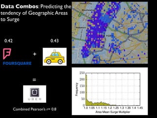
![Surge Prediction
import scipy.stats as stats
yellows = [TAXIcellCount[cy][cx] for cy in range(0, latLen-1) for cx in range(0,lonLen-1) if
latLongSurge[cy][cx] !=0]
places = [FSQcellCount[cy][cx] for cy in range(0, latLen-1) for cx in range(0,lonLen-1) if
latLongSurge[cy][cx] !=0]
listings = [AIRcellCount[cy][cx] for cy in range(0, latLen-1) for cx in range(0,lonLen-1) if
latLongSurge[cy][cx] !=0]
cnt = 0
labels = ['Yellow Taxis', 'Foursquare Places', 'Airbnb Listings']
print len(surgeValues)
print len(yellows)
for predictor in [yellows, places, listings]:
r, p_value = stats.pearsonr(surgeValues, predictor)
Yellow Taxis
0.432527851946
---
Foursquare Places
0.407164228291
---
Airbnb Listings
0.327540653569](https://image.slidesharecdn.com/pydataslidesmininggeoreferneddatanoulas-151110021020-lva1-app6892/85/Mining-Geo-referenced-Data-Location-based-Services-and-the-Sharing-Economy-37-320.jpg)
![Supervised learning for Surge prediction
from sklearn import tree
y_train = [] #a list for your training labels
X_train = [] #feature values go here
for i in range(0, len(surgeValues)):
y_train.append(surgeValues[i])
X_train.append([yellows[i], listings[i], places[i]])
print 'Training Decision Tree Regressor..'
### Training and Testing: LEAVE ONE OUT ERROR ####
super_predictions = []
super_predictions2 = []
for i in range(0, len(surgeValues)):
training_data_X = X_train[:i] + X_train[i+1:]
label_data_Y = y_train[:i] + y_train[i+1:]
NX_train = []
ny_train = []
for j in range(0, len(label_data_Y)):
if label_data_Y[j] == 1.0:
continue
else:
NX_train.append(X_train[j])
ny_train.append(y_train[j])
clf = tree.DecisionTreeRegressor(max_depth=30).fit(NX_train, ny_train)
super_predictions.append(clf.predict(X_train[i])[0])
r, p_value = stats.pearsonr(surgeValues, super_predictions)
print 'Decision Tree Supervised Learning Regressor, r :' + str(r)](https://image.slidesharecdn.com/pydataslidesmininggeoreferneddatanoulas-151110021020-lva1-app6892/85/Mining-Geo-referenced-Data-Location-based-Services-and-the-Sharing-Economy-38-320.jpg)


![Using arc map to create package map along with a report file [metadata]](https://cdn.slidesharecdn.com/ss_thumbnails/usingarcmaptocreatepackagemapalongwithareportfilemetadata-140430025951-phpapp02-thumbnail.jpg?width=640&height=640&fit=bounds)