The binary search algorithm allows for faster searching of an ordered array compared to linear search. It works by first examining the middle element of the array and eliminating half of the elements from further search based on whether the target value is less than or greater than the middle element. This process continues, halving the search space on each iteration, allowing binary search to have a time complexity of O(log n).

1. Explanation of binary search algorithm
Suppose we are given a number of integers stored in an array A, and we want to locate a specific target integer K
in this array. If we do not have any information on how the integers are organized in the array, we have to
sequentially examine each element of the array. This is known as linear search and would have a time complexity
of O(n ) in the worst case. However, if the elements of the array are ordered, let us say in ascending order, and we
wish to find out the position of an integer target K in the array, we need not make a sequential search over the
complete array. We can make a faster search using the Binary search method. The basic idea is to start with an
examination of the middle element of the array. This
will lead to 3 possible situations:
If this matches the target K then search can terminate successfully by printing out the index of the element in the
array. On the other hand, if K<A[middle], then search can be limited to elements to the left of A[middle]. All
elements to the right of middle can be ignored. If it turns out that K >A[middle], then further search is limited to
elements to the right of A[middle]. If all elements are exhausted and the target is not found in the array, then the
method returns a special value such as –1. Here is one version of the Binary Search function:
int BinarySearch (int A[ ], int n, int K)
{
int L=0, Mid, R= n-1;
while (L<=R)
{
Mid = (L +R)/2;
if ( K= =A[Mid] )
return Mid;
else if ( K > A[Mid] )
L = Mid + 1;
else
R = Mid – 1 ;
}
return –1 ;
}
Let us now carry out an Analysis of this method to determine its time complexity. Since there are no “for” loops,
we can not use summations to express the total number of operations. Let us examine the operations for a specific
case, where the number of elements in the array n is 64. When n= 64 Binary Search is called to reduce size to n=32.
When n= 32 Binary Search is called to reduce size to n=16
When n= 16 Binary Search is called to reduce size to n=8
When n= 8 Binary Search is called to reduce size to n=4
When n= 4 Binary Search is called to reduce size to n=2
When n= 2 Binary Search is called to reduce size to n=1
Thus we see that Binary Search function is called 6 times ( 6 elements of the array were examined) for n =64. Note
6
that 64 = 2 . Also we see that the Binary Search function is called 5 times ( 5 elements of the array were examined)
5 k
for n = 32. Note that 32 = 2 . Let us consider a more general case where n is still a power of 2. Let us say n = 2 .
Following the above argument for 64 elements, it is easily seen that after k searches, the while loop is executed k
times and n reduces to size 1. Let us assume that each run of the while loop involves at most 5 operations. Thus
k
total number of operations: 5k. The value of k can be determined from the expression 2 = n. Taking log of both
sides k = log n. Thus total number of operations = 5 log n. We conclude from there that the time complexity of the
Binary search method is O(log n), which is much more efficient than the Linear Search method.
Show that clique problem is an NP complete problem
Clique Problem:-In computer science, the clique problem refers to any of the problems related to
finding particular complete sub graphs in a graph, i.e., sets of elements where each pair of elements is
connected. For example, the maximum clique problem arises in the following real-world setting.
Consider a social network, where the graph’s vertices represent people, and the graph’s edges represent
mutual acquaintance. To find a largest subset of people who all know each other, one can systematically
inspect all subsets, a process that is too time-consuming to be practical for social networks comprising

2. more than a few dozen people. Although this brute-force search can be improved by more
efficient algorithms, all of these algorithms take exponential time to solve the problem. Therefore, much
of the theory about the clique problem is devoted to identifying special types of graph that admit more
efficient algorithms, or to establishing the computational difficulty of the general problem in various
models of computation.
Clique problem is an NP complete The clique decision problem is NP-complete. This problem was also
mentioned in Stephen Cook's paper introducing the theory of NP-complete problems. Thus, the problem
of finding a maximum clique is NP-hard: if one could solve it, one could also solve the decision problem,
by comparing the size of the maximum clique to the size parameter given as input in the decision
problem. Karp's NP-completeness proof is a many-one reduction from the Boolean satisfiability
problem for formulas in conjunctive normal form, which was proved NP-complete in the Cook–Levin
theorem. From a given CNF formula, Karp forms a graph that has a vertex for every pair (v,c), where v is
a variable or its negation and c is a clause in the formula that contains v. Vertices are connected by an
edge if they represent compatible variable assignments for different clauses: that is, there is an edge
from (v,c) to (u,d) whenever c ≠ d and u and v are not each others' negations. Ifk denotes the number of
clauses in the CNF formula, then the k-vertex cliques in this graph represent ways of assigning truth
values to some of its variables in order to satisfy the formula; therefore, the formula is satisfiable if and
only if a k-vertex clique exists.
Some NP-complete problems (such as the travelling salesman problem in planar graphs) may be solved
in time that is exponential in a sublinear function of the input size parameter n. However,
as Impagliazzo, Paturi & Zane (2001)describe, it is unlikely that such bounds exist for the clique problem
in arbitrary graphs, as they would imply similarly subexponential bounds for many other standard NP-
complete problems.
A monotone circuit to detect a k-clique in an n-vertex graph for k = 3 and n = 4.
Each of the 6 inputs encodes the presence or absence of a particular (red) edge in the input graph. The circuit uses one
internal or-gate to detect each potential k-clique.
According to the CHOMSKY’s what are the different types in which grammars are classified? Explain with an
example
Within the field of computer science, specifically in the area of formal languages, the Chomsky hierarchy is
a containment hierarchy of classes of formal grammars.
 Type-0 grammars (unrestricted grammars) include all formal grammars. They generate exactly all languages
that can be recognized by a Turing machine. These languages are also known as the recursively enumerable
languages. Note that this is different from the recursive languages which can be decided by an always-halting
Turing machine.
 Type-1 grammars (context-sensitive grammars) generate the context-sensitive languages. These grammars
have rules of the form with A a nonterminal and α, β and γ strings of terminals and
nonterminals. The strings α and β may be empty, but γ must be nonempty. The rule is allowed
if S does not appear on the right side of any rule. The languages described by these grammars are exactly all
languages that can be recognized by a linear bounded automaton (a nondeterministic Turing machine whose
tape is bounded by a constant times the length of the input.)

3.  Type-2 grammars (context-free grammars) generate the context-free languages. These are defined by rules of
the form with A a nonterminal and γ a string of terminals and nonterminals. These languages are
exactly all languages that can be recognized by a non-deterministic pushdown automaton. Context-free
languages are the theoretical basis for the syntax of most programming languages.
 Type-3 grammars (regular grammars) generate the regular languages. Such a grammar restricts its rules to a
single nonterminal on the left-hand side and a right-hand side consisting of a single terminal, possibly followed
(or preceded, but not both in the same grammar) by a single nonterminal. The rule is also allowed
here if S does not appear on the right side of any rule. These languages are exactly all languages that can be
decided by a finite state automaton. Additionally, this family of formal languages can be obtained by regular
expressions. Regular languages are commonly used to define search patterns and the lexical structure of
programming languages.
Production rules
Grammar Languages Automaton
(constraints)
Recursively
Type-0 Turing machine (no restrictions)
enumerable
Linear-bounded non-deterministic Turing
Type-1 Context-sensitive αAβ ⟶ αγβ
machine
Type-2 Context-free Non-deterministic pushdown automaton
Type-3 Regular Finite state automaton and
Greedy algorithm gives a optimal solution & when it will be failed
A greedy algorithm is any algorithm that follows the problem solving heuristic of making the locally
optimal choice at each stage with the hope of finding the global optimum. For example, applying the
greedy strategy to the traveling salesman problem yields the following algorithm: "At each stage visit
the unvisited city nearest to the current city". In general, greedy algorithms are used for optimization
problems. In general, greedy algorithms have five pillars:
1. A candidate set, from which a solution is created
2. A selection function, which chooses the best candidate to be added to the solution
3. A feasibility function, that is used to determine if a candidate can be used to contribute to a
solution
4. An objective function, which assigns a value to a solution, or a partial solution, and
5. A solution function, which will indicate when we have discovered a complete solution
Greedy algorithms produce good solutions on some mathematical problems, but not on others. Most
problems for which they work, will have two properties:
Greedy choice property:-
We can make whatever choice seems best at the moment and then solve the subproblems that
arise later. The choice made by a greedy algorithm may depend on choices made so far but not
on future choices or all the solutions to the subproblem. It iteratively makes one greedy choice
after another, reducing each given problem into a smaller one. In other words, a greedy
algorithm never reconsiders its choices. This is the main difference from dynamic programming,
which is exhaustive and is guaranteed to find the solution. After every stage, dynamic
programming makes decisions based on all the decisions made in the previous stage, and may
reconsider the previous stage's algorithmic path to solution.
Cases of failure:-
For many other problems, greedy algorithms fail to produce the optimal solution, and may even produce
the unique worst possible solution. One example is the traveling salesman problem mentioned above:

4. for each number of cities there is an assignment of distances between the cities for which the nearest
neighbor heuristic produces the unique worst possible tour.
Imagine the coin example with only 25-cent, 10-cent, and 4-cent coins. The greedy algorithm would not
be able to make change for 41 cents, since after committing to use one 25-cent coin and one 10-cent
coin it would be impossible to use 4-cent coins for the balance of 6 cent. Whereas a person or a more
sophisticated algorithm could make change for 41 cents change with one 25-cent coin and four 4-cent
coins.
Give an analysis of Best first search
Best-first search is a search algorithm which explores a graph by expanding the most promising node chosen
according to a specified rule. Judea Pearl described best-first search as estimating the promise of node n by a
"heuristic evaluation function f(n) which, in general, may depend on the description of n, the description of the
goal, the information gathered by the search up to that point, and most important, on any extra knowledge about
the problem domain." Some authors have used "best-first search" to refer specifically to a search with
a heuristic that attempts to predict how close the end of a path is to a solution, so that paths which are judged to
be closer to a solution are extended first. This specific type of search is called greedy best-first search. Efficient
selection of the current best candidate for extension is typically implemented using a priority queue.
The A* search algorithm is an example of best-first search. Best-first algorithms are often used for path finding
in combinatorial search. There are a whole batch of heuristic search algorithm e.g. hill climbing search, best first
search, A*, AO* etc. A* uses a best-first search and finds the least-cost path from a given initial node to one goal
node. It uses a distance-plus-cost heuristic function (usually denoted f(x)) to determine the order in which the
search visits nodes in the tree. The distance-plus-cost heuristic is a sum of two functions:
 the path-cost function, which is the cost from the starting node to the current node (usually denoted g(x))
 and an admissible "heuristic estimate" of the distance to the goal (usually denoted h(x)).
The h(x) part of the f(x) function must be an admissible heuristic; that is, it must not overestimate the distance to
the goal. Thus, for an application like routing, h(x) might represent the straight-line distance to the goal, since that
is physically the smallest possible distance between any two points or nodes.
If the heuristic h satisfies the additional condition for every edge x, y of the graph
(where d denotes the length of that edge), then h is called monotone, or consistent. In such a case, A* can be
implemented more efficiently—roughly speaking, no node needs to be processed more than once (see closed
set below)—and A* is equivalent to running Dijkstra's algorithm with the reduced cost d'(x,y): = d(x,y) − h(x) + h(y).
We'll describe the best-first algorithm in terms of a specific example involving distances by straight line and by
road from a start point s to a goal point t:

5. Let us define, for any node N, g(N) to be the distance travelled from the start node s to reach N. Note that this is a
known quantity by the time you reach N, but that in general it could vary depending on the route taken through
state space from s to N.
In our example scenario, we don't know the distance by road from N to t, but we do know the straight-line
distance. Let us call this distance h(N). As our heuristic to guide best-first search, we use f(N) = g(N) + h(N). That is,
we will search first from the node that we have found so far that has the lowest f(N).
What is the benefit of preconditioning a problem space? Explain with example
Preconditioning is preparing the problem space before application of the algorithm.
For example: in binary search the searching technique can only be applied on a sorted array. Similarly heap sort
requires data to be organized in the form of heap, before sorting technique can be applied. This is called
preconditioning of the data.
Design a NDF automata or NDFA representing the language over alphabet ={a, b} in which all valid strings have
bb or bab as sub string
a,b a,b
0 b 1 b 3
a b
2
in quick sort average cost is closer to best case than worst case- comment
In quick sort the average case complexity is O(n log n).
The best case is obtained if the pivot point is always the mid position, which gives the complexity O(n log n).
2
The worst case complexity is O(n ) when the array is already sorted.
Hence the average case is closer to the best case
Describe whether or not breadth first search algorithm always finds the shortest path to a selected vertex from
the starting vertex
Algorithm of BFS
procedure BFS(Graph,v):
2 create a queue Q
3 enqueue v onto Q
4 mark v
5 while Q is not empty:
6 t ← Q.dequeue()
7 for all edges e in G.incidentEdges(t) do
8 o ← G.opposite(v,e)
9 if o is not marked:
10 mark o
11 enqueue o onto Q
Limitation of Strassen's Algorithm
From a practical point of view Strassen's Algorithm is often not the method of choice for matrix multiplication for
the following four reasons:
(1) The constant factor hidden in the running time Strassen's Algorithm is lager than the constant factor in
the native (n ) method.
3

6. (2) When the matrices are sparse method tailored for sparse matrices are faster.
(3) Strassen's Algorithm is not quite as numerically stable as the native method.
(4) The sub matrices formed at the level of consume space.
Describe white path property of DFS
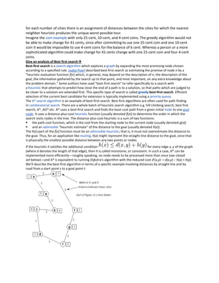
In a DFS forest of a (directed or undirected) graph G, vertex v is a descendant of vertex u if and only if at time s[u]
(just before u is colored Gray), there is a path from u to v that consists of only White vertices. Proof there are two
directions to prove.
(=⇒ Suppose that v is a descendant of u. So there is a path in the tree from u to v. (Of course this is also a path in
)
G.) All vertices w on this path are also descendants of u. So by the corollary above, they are colored Gray during
the interval [s[u], f[u]]. In other words, at time s[u] they are all White.
(⇐ Suppose that there is a White path from u to v at time s[u]. Let this path be v0 = u, v1, v2, . . . , vk−1, vk = v
=)
To show that v is a descendant of u, we will indeed show that all vi (for 0 ≤ i ≤ k) are descendants of u. (Note that
this path may not be in the DFS tree.) We prove this claim by induction on i.
Base case: i = 0, vi = u, so the claim is obviously true.
Induction step: Suppose that vi is a descendant of u. We show that vi+1 is also a descendant of u. By the corollary
above, this is equivalent to showing that
s[u] < s[vi+1] < f[vi+1] < f[u] i.e., vi+1 is colored Gray during the interval [s[u], f[u]]. Since vi+1 is White at time s[u],
we have s[u] < s[vi+1]. Now, since vi+1 is a neighbor of vi, vi+1 cannot stay White after vi is colored Black. In other
words, s[vi+1] < f[vi]. Apply the induction hypothesis: vi is a descendant of u so s[u] ≤ s[vi] < f[vi] ≤ f[u], we obtain
s[vi+1] < f[u]. Thus s[u] < s[vi+1] < f[vi+1] < f[u] by the Parenthesis Theorem. QED.
In a quick sort algorithm describe the situation when a given pair of elements will be compared to each other &
when they will not compared to each other
Even if pivots aren't chosen randomly, quicksort still requires only O(n log n) time averaged over all possible
permutations of its input. Because this average is simply the sum of the times over all permutations of the input
divided by n factorial, it's equivalent to choosing a random permutation of the input. When we do this, the pivot
choices are essentially random, leading to an algorithm with the same running time as randomized quicksort.
More precisely, the average number of comparisons over all permutations of the input sequence can be estimated
accurately by solving the recurrence relation:
Here, n − 1 is the number of comparisons the partition uses. Since the pivot is equally likely to fall anywhere in the
sorted list order, the sum is averaging over all possible splits.
This means that, on average, quicksort performs only about 39% worse than in its best case. In this sense it is
closer to the best case than the worst case. Also note that a comparison sort cannot use less
than log 2(n!) comparisons on average to sort n items and in case of large n, Stirling's
approximation yields , so quicksort is not much worse than an ideal
comparison sort. This fast average runtime is another reason for quicksort's practical dominance over other
sorting algorithms.
Among BDS & DFS which technique is used in ignorer traversal a Binary tree & how? 
The BFS can be used in order traversal of a Binary tree. BFS is a little like hill climbing, in that it uses an evaluation
function & always chooses the next node to be that with the best score. However it is exhaustive in that it should
eventually try all possible paths. The BFS algorithm was developed to simulate the various client based spiders
developed in earlier studies & were used as benchmark for comparison. The genetic algorithm was adopted to
enhance the global optimal search capability of existing internet spider.
Define pumping lemma for context free grammar
In the theory of formal languages in computability theory, a pumping lemma or pumping argument states that, for
a particular language to be a member of a language class, any sufficiently long string in the language contains a
section, or sections, that can be removed, or repeated any number of times, with the resulting string remaining in
that language. The proofs of these lemmas typically require counting arguments such as the pigeonhole principle.
The two most important examples are the pumping lemma for regular languages and the pumping lemma for
context-free languages. Ogden's lemma is a second, stronger pumping lemma for context-free languages

7. Construct a finite Automata for the language: a*(ab+ba)b*
Construct a non deterministic finite automata represented the language (ab)*(ba)+aa*
Write a Context free grammar for a non null even palindrome
In automata theory a set of all palindromes in a given alphabet is a typical example of a language which is context
free but not regular. The following context free grammar produces all palindromes for alphabet {a, b}:S
a|b|aSa|bSb|(empty)
Discuss how DFS can be search can be used to find cycles in an undirected graph
Given an undirected graph a DFS algorithm construct a directed tree from the root. If there exists a directed path
in the tree from v to w then v is a predecessor of w is a descendant of v. a node adjacency structure is an n*n
matrix such that entry aij=1 if node 1 is adjacent to node j & 0 otherwise. A node edge adjacency structure lists for
each node, the nodes adjacent to it.
Write a recursive procedure to compute the factorial of a given number
int fact(int n)
{
if (n=1)then
{
return 1;
}
else
{
Result=n*fact(n-1);
}
}
Properties of good dynamic programming problem
1. The problem can be divided into stages with a decision required at each stage.
In the capital budgeting problem the stages were the allocations to a single plant. The decision was how
much to spend. In the shortest path problem, they were defined by the structure of the graph. The decision
was to go next.
2. Each stage has a number of states associated with it.

8. The states for the capital budgeting problem corresponded to the amount spent at that point in time. The
states for the shortest path problem were the node reached.
3. The decision at one stage transforms one state into a state in the next stage.
The decision of how much to spend gave a total amount spent for the next stage. The decision of where to
go next defined where you arrived in the next stage.