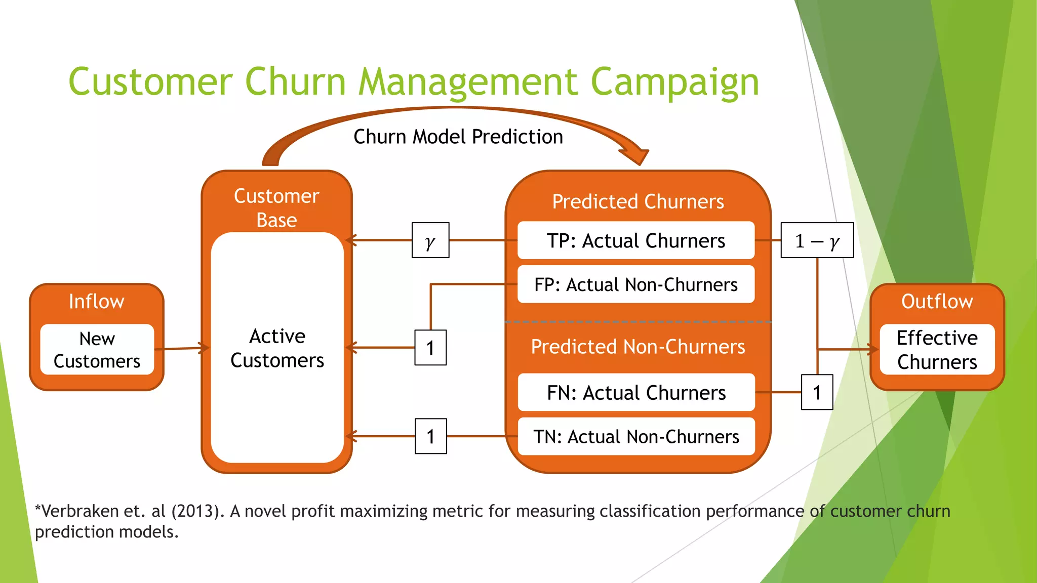
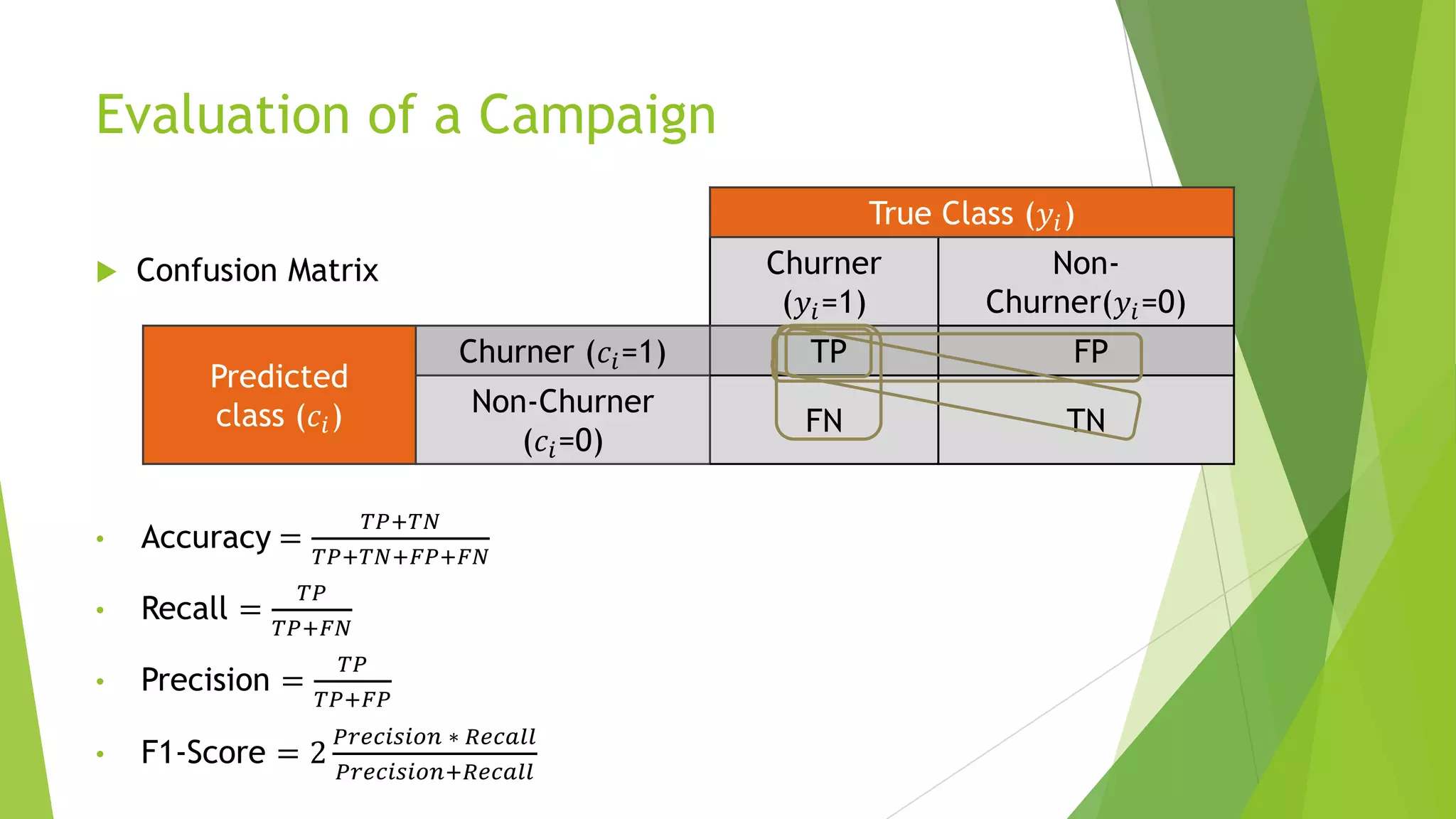
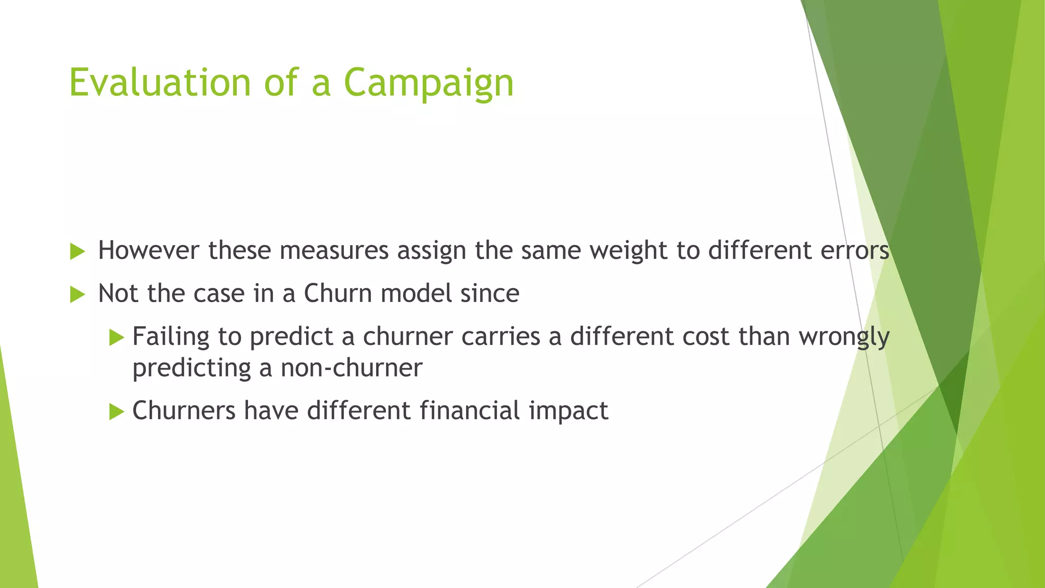
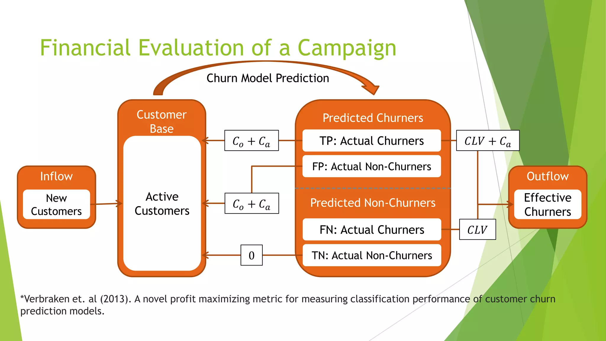
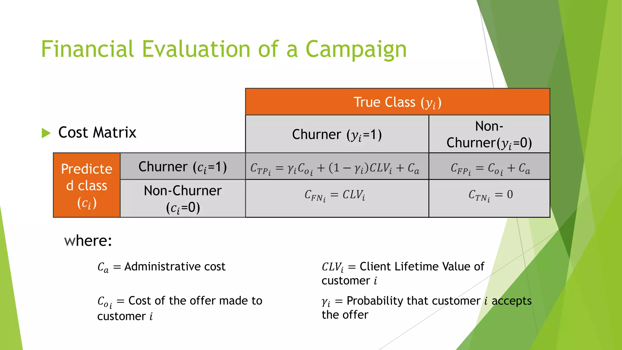
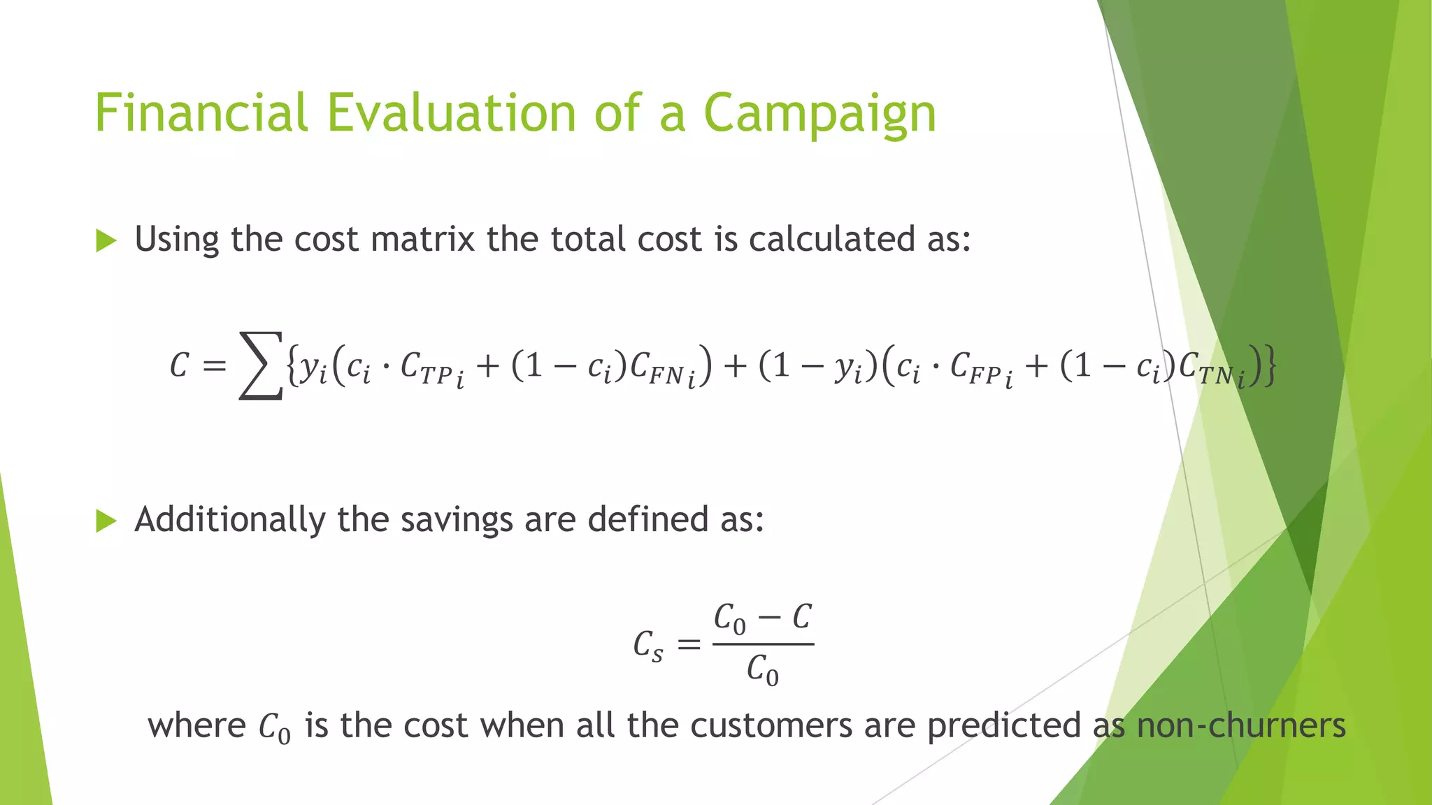
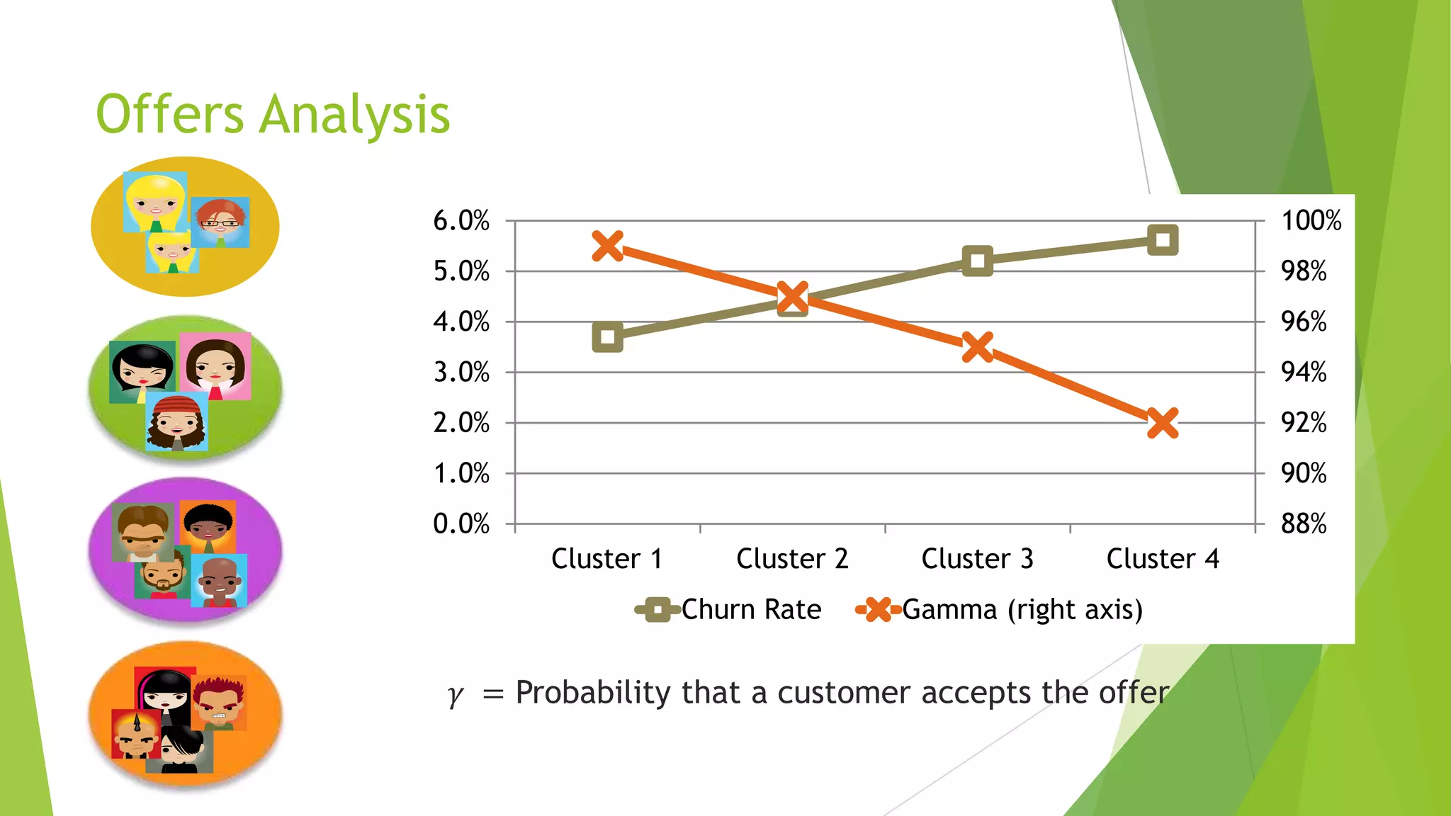
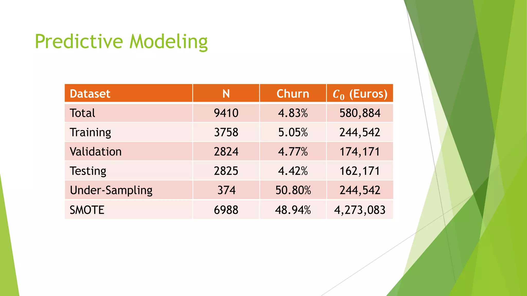
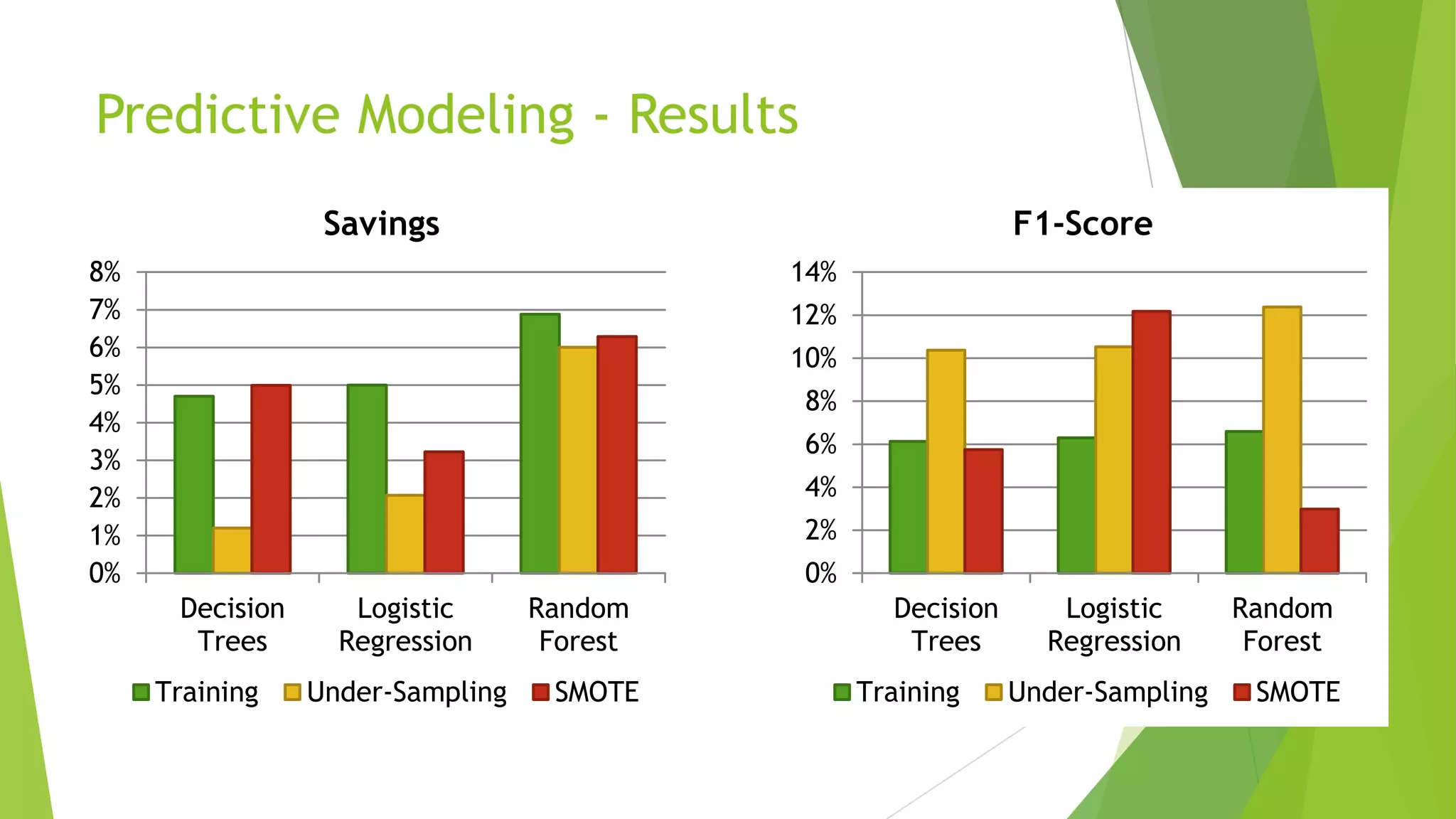
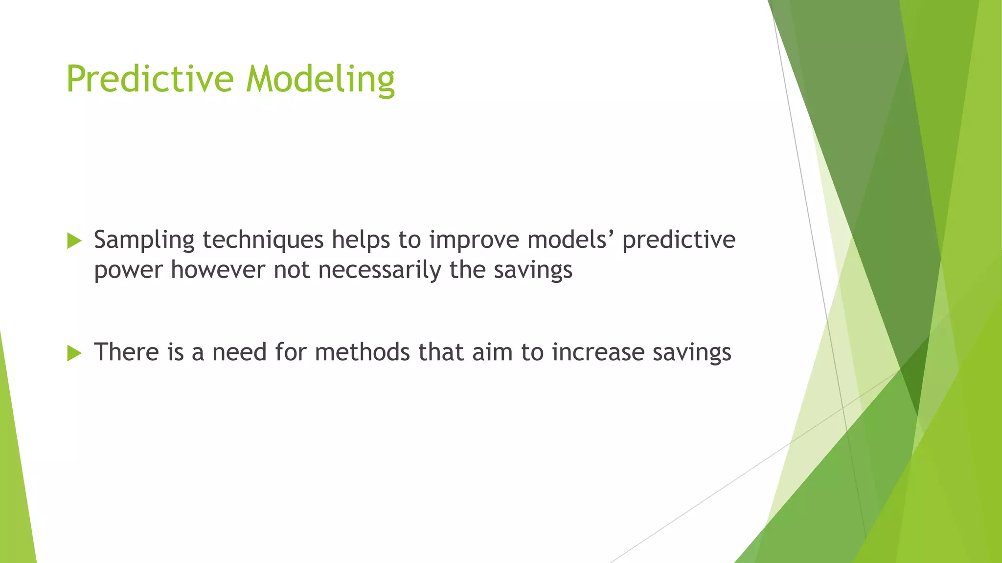
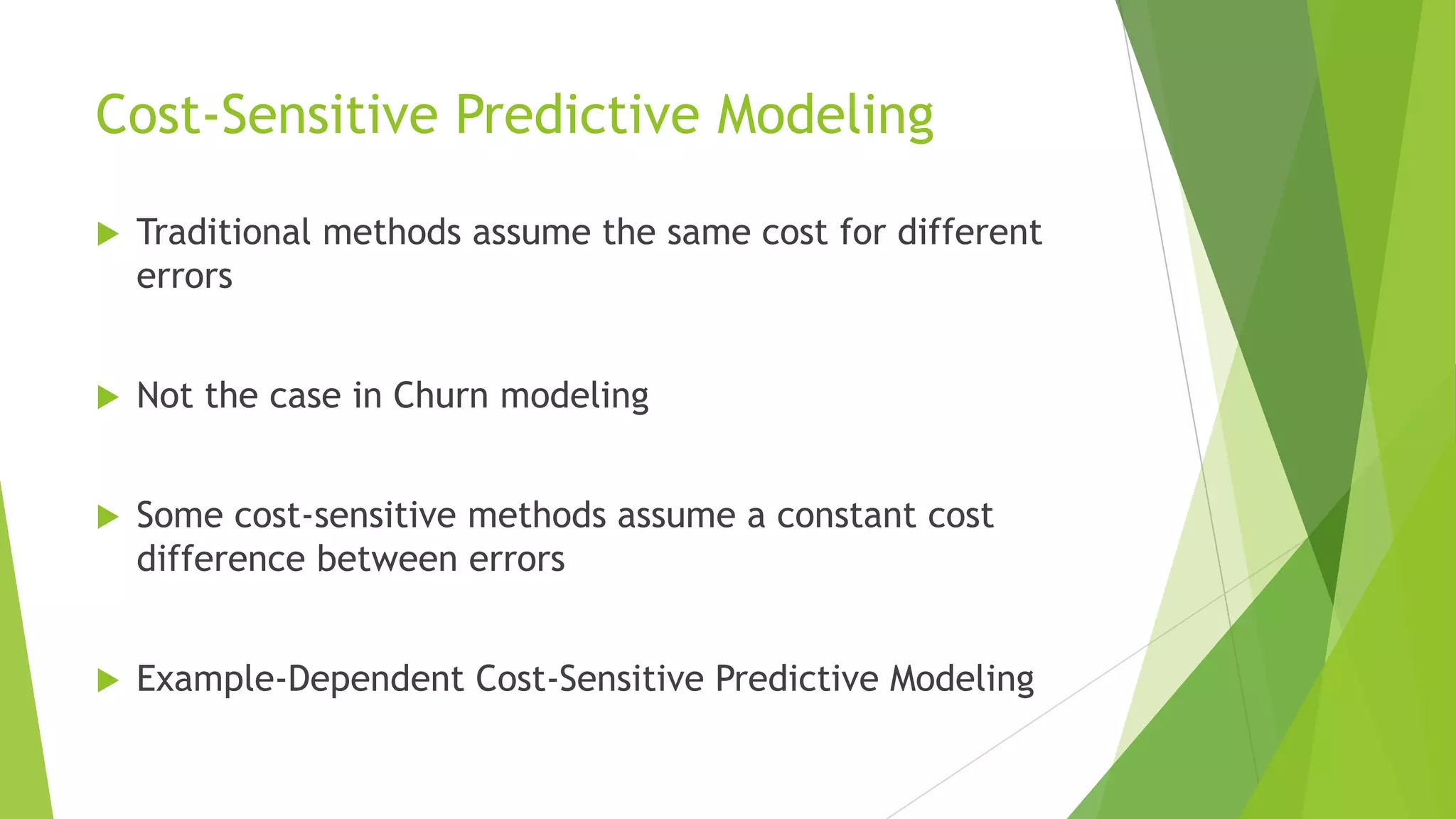
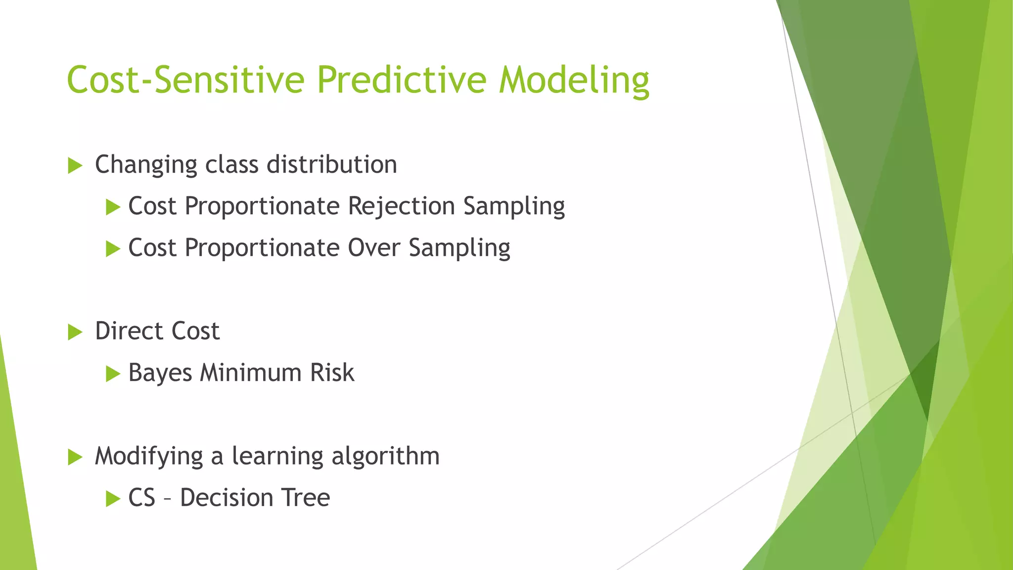
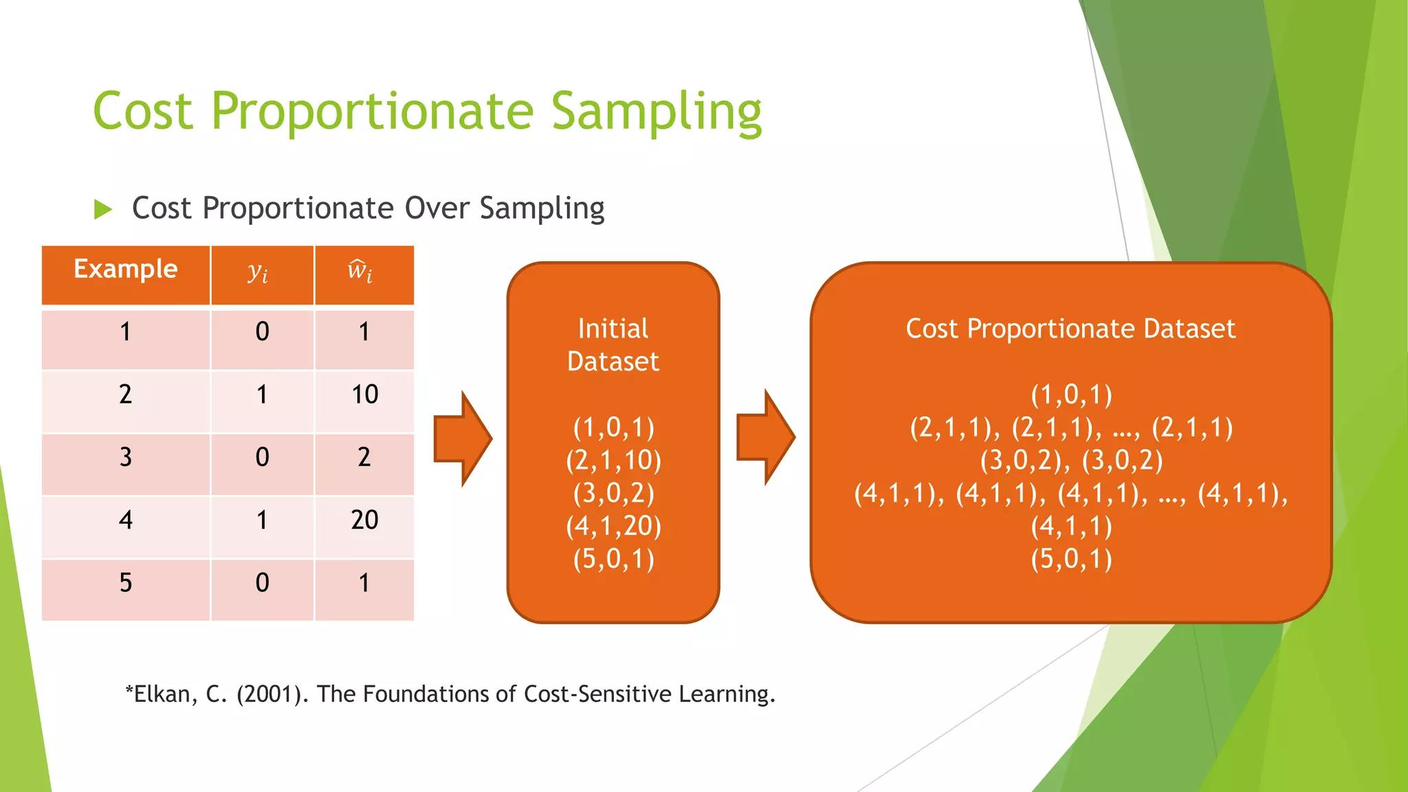
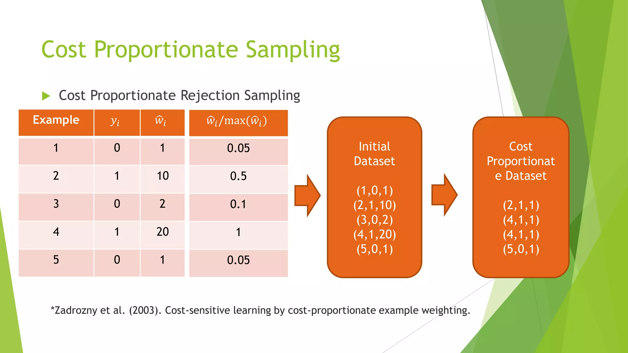
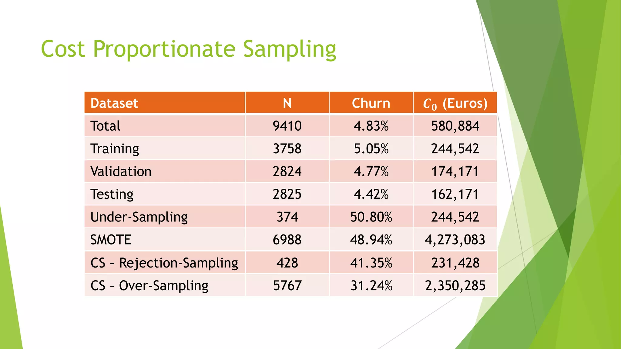
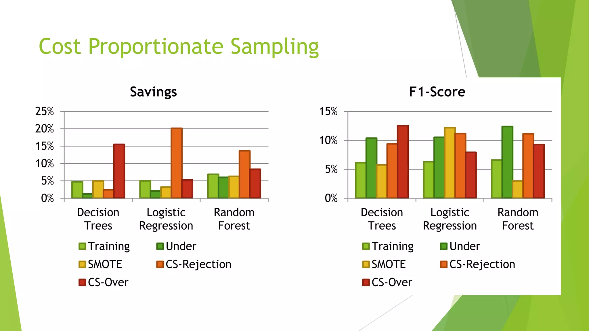
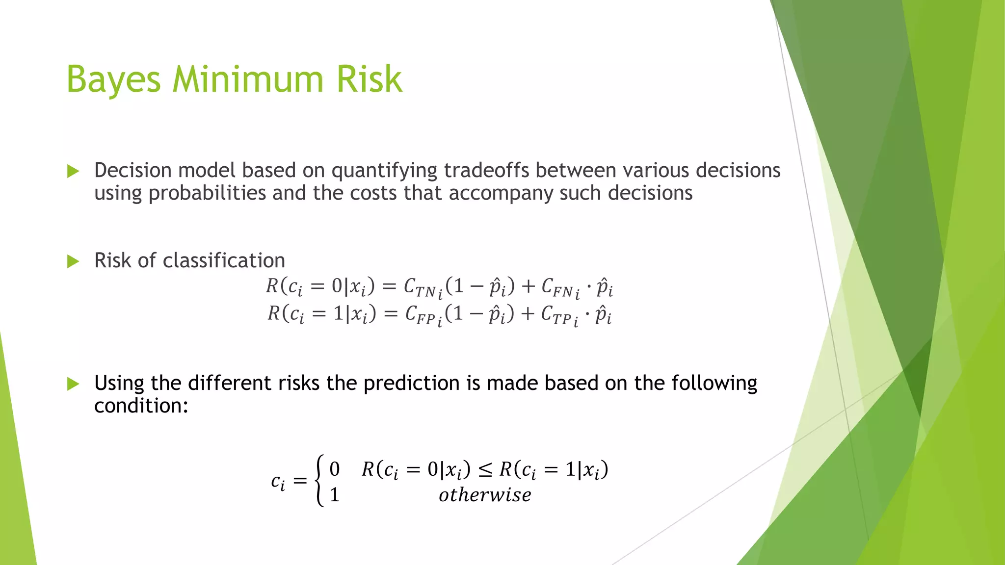
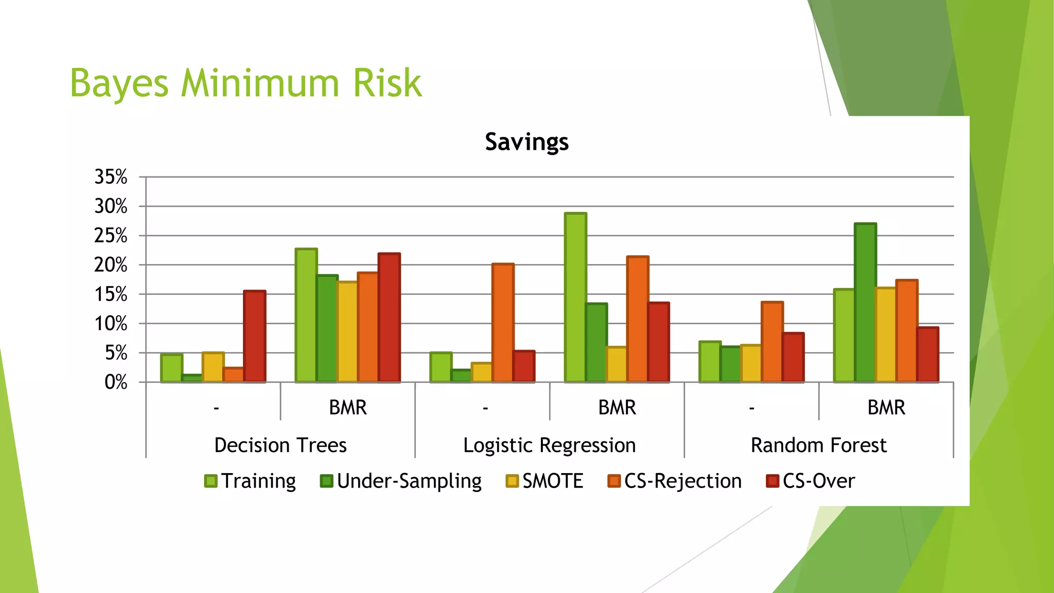
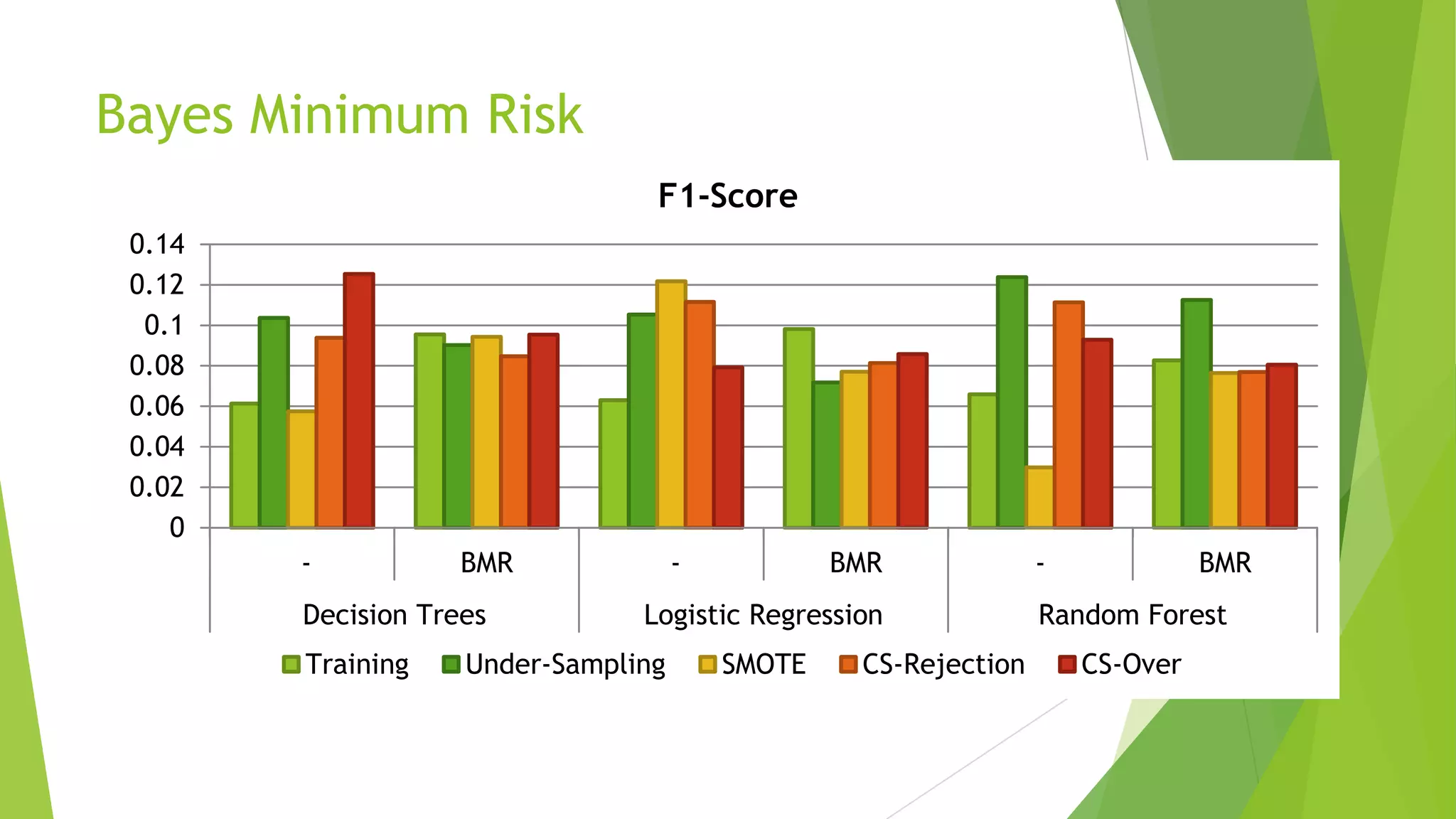
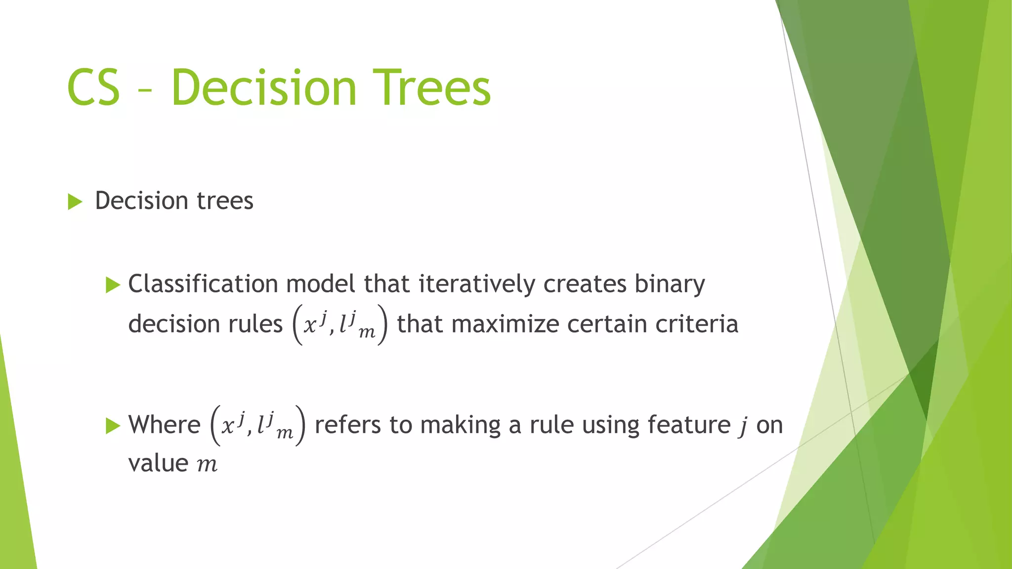
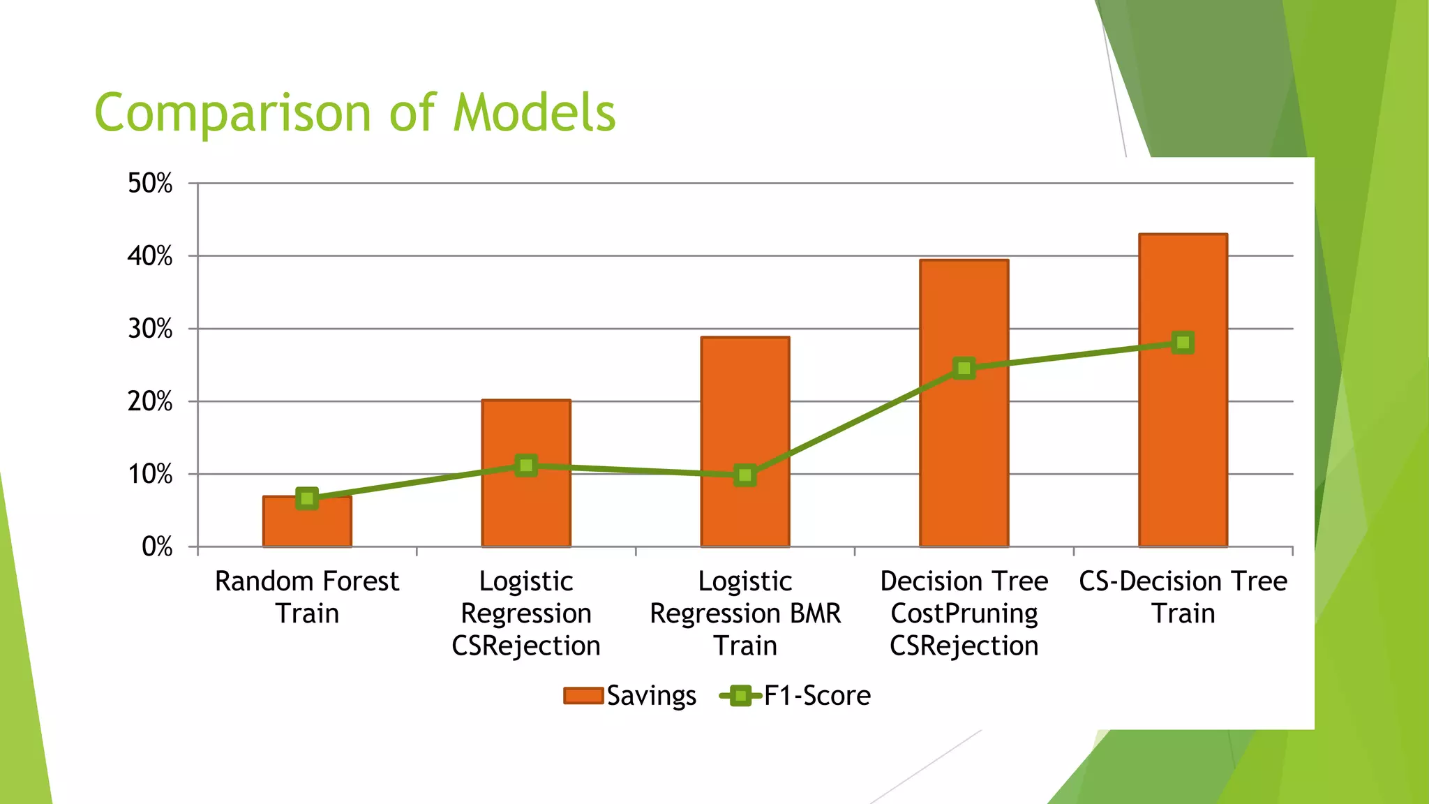
Maximizing a churn
campaign’s profitability
with cost sensitive
machine learning
Alejandro Correa Bahnsen, PhD
Chief Data Scientist | Easy Solutions
Agosto 25 y 26 | Lima – Perú 2017
#BIGDATASUMMIT2017
Agenda
 Churn modeling
 Evaluation Measures
 Offers
 Predictive modeling
 Cost-Sensitive Predictive Modeling
 Cost Proportionate Sampling
 Bayes Minimum Risk
 CS – Decision Trees
 Conclusions
Churn Modeling
• Detect which customers are likely to abandon
Voluntary churn
Involuntary churn
Customer Churn Management Campaign
Inflow
New
Customers
Customer
Base
Active
Customers
*Verbraken et. al (2013). A novel profit maximizing metric for measuring classification performance of customer churn
prediction models.
Predicted Churners
Predicted Non-Churners
TP: Actual Churners
FP: Actual Non-Churners
FN: Actual Churners
TN: Actual Non-Churners
Outflow
Effective
Churners
Churn Model Prediction
1
1
1 − 𝛾𝛾
1
Evaluation of a Campaign
 Confusion Matrix
• Accuracy =
𝑇𝑃+𝑇𝑁
𝑇𝑃+𝑇𝑁+𝐹𝑃+𝐹𝑁
• Recall =
𝑇𝑃
𝑇𝑃+𝐹𝑁
• Precision =
𝑇𝑃
𝑇𝑃+𝐹𝑃
• F1-Score = 2
𝑃𝑟𝑒𝑐𝑖𝑠𝑖𝑜𝑛 ∗ 𝑅𝑒𝑐𝑎𝑙𝑙
𝑃𝑟𝑒𝑐𝑖𝑠𝑖𝑜𝑛+𝑅𝑒𝑐𝑎𝑙𝑙
True Class (𝑦𝑖)
Churner
(𝑦𝑖=1)
Non-
Churner(𝑦𝑖=0)
Predicted
class (𝑐𝑖)
Churner (𝑐𝑖=1) TP FP
Non-Churner
(𝑐𝑖=0)
FN TN
Evaluation of a Campaign
 However these measures assign the same weight to different errors
 Not the case in a Churn model since
 Failing to predict a churner carries a different cost than wrongly
predicting a non-churner
 Churners have different financial impact
Financial Evaluation of a Campaign
Inflow
New
Customers
Customer
Base
Active
Customers
*Verbraken et. al (2013). A novel profit maximizing metric for measuring classification performance of customer churn
prediction models.
Predicted Churners
Predicted Non-Churners
TP: Actual Churners
FP: Actual Non-Churners
FN: Actual Churners
TN: Actual Non-Churners
Outflow
Effective
Churners
Churn Model Prediction
0
𝐶𝐿𝑉
𝐶𝐿𝑉 + 𝐶 𝑎𝐶 𝑜 + 𝐶 𝑎
𝐶 𝑜 + 𝐶 𝑎
Financial Evaluation of a Campaign
 Cost Matrix
where:
True Class (𝑦𝑖)
Churner (𝑦𝑖=1)
Non-
Churner(𝑦𝑖=0)
Predicte
d class
(𝑐𝑖)
Churner (𝑐𝑖=1)
Non-Churner
(𝑐𝑖=0)
𝐶 𝑎 = Administrative cost 𝐶𝐿𝑉𝑖 = Client Lifetime Value of
customer 𝑖
𝐶𝑜 𝑖
= Cost of the offer made to
customer 𝑖
𝛾𝑖 = Probability that customer 𝑖 accepts
the offer
𝐶 𝑇𝑃 𝑖
= 𝛾𝑖 𝐶 𝑜 𝑖
+ 1 − 𝛾𝑖 𝐶𝐿𝑉𝑖 + 𝐶 𝑎
𝐶 𝐹𝑁 𝑖
= 𝐶𝐿𝑉𝑖 𝐶 𝑇𝑁 𝑖
= 0
𝐶 𝐹𝑃 𝑖
= 𝐶 𝑜 𝑖
+ 𝐶 𝑎
Financial Evaluation of a Campaign
 Using the cost matrix the total cost is calculated as:
𝐶 = 𝑦𝑖 𝑐𝑖 ∙ 𝐶 𝑇𝑃 𝑖 + 1 − 𝑐𝑖 𝐶 𝐹𝑁 𝑖 + 1 − 𝑦𝑖 𝑐𝑖 ∙ 𝐶 𝐹𝑃 𝑖 + 1 − 𝑐𝑖 𝐶 𝑇𝑁 𝑖
 Additionally the savings are defined as:
𝐶𝑠 =
𝐶0 − 𝐶
𝐶0
where 𝐶0 is the cost when all the customers are predicted as non-churners
Financial Evaluation of a Campaign
 Customer Lifetime Value
*Glady et al. (2009). Modeling churn using customer lifetime value.
Offers
 Same offer may not apply to all customers (eg. Already
have premium channels)
 An offer should be made such that it maximizes the
probability of acceptance (𝛾)
Offers Analysis
Improve
to HD
DVR
Monthly
Discount
Premium
Channels
Evaluate
Offers
Performance
Offers Analysis
88%
90%
92%
94%
96%
98%
100%
0.0%
1.0%
2.0%
3.0%
4.0%
5.0%
6.0%
Cluster 1 Cluster 2 Cluster 3 Cluster 4
Churn Rate Gamma (right axis)
𝛾 = Probability that a customer accepts the offer
Predictive Modeling
Dataset N Churn 𝑪 𝟎 (Euros)
Total 9410 4.83% 580,884
Training 3758 5.05% 244,542
Validation 2824 4.77% 174,171
Testing 2825 4.42% 162,171
SMOTE 6988 48.94% 4,273,083
Under-Sampling 374 50.80% 244,542
Predictive Modeling
 Algorithms
 Decision Trees
 Logistic Regression
 Random Forest
Predictive Modeling - Results
0%
2%
4%
6%
8%
10%
12%
14%
Decision
Trees
Logistic
Regression
Random
Forest
F1-Score
Training Under-Sampling SMOTE
0%
1%
2%
3%
4%
5%
6%
7%
8%
Decision
Trees
Logistic
Regression
Random
Forest
Savings
Training Under-Sampling SMOTE
Predictive Modeling
 Sampling techniques helps to improve models’ predictive
power however not necessarily the savings
 There is a need for methods that aim to increase savings
Agenda
 Churn modeling
 Evaluation Measures
 Offers
 Predictive modeling
 Cost-Sensitive Predictive Modeling
 Cost Proportionate Sampling
 Bayes Minimum Risk
 CS – Decision Trees
 Conclusions
Cost-Sensitive Predictive Modeling
 Traditional methods assume the same cost for different
errors
 Not the case in Churn modeling
 Some cost-sensitive methods assume a constant cost
difference between errors
 Example-Dependent Cost-Sensitive Predictive Modeling
Cost-Sensitive Predictive Modeling
 Changing class distribution
 Cost Proportionate Rejection Sampling
 Cost Proportionate Over Sampling
 Direct Cost
 Bayes Minimum Risk
 Modifying a learning algorithm
 CS – Decision Tree
Cost Proportionate Sampling
 Cost Proportionate Over Sampling
Example 𝑦𝑖 𝑤𝑖
1 0 1
2 1 10
3 0 2
4 1 20
5 0 1
Initial
Dataset
(1,0,1)
(2,1,10)
(3,0,2)
(4,1,20)
(5,0,1)
Cost Proportionate Dataset
(1,0,1)
(2,1,1), (2,1,1), …, (2,1,1)
(3,0,2), (3,0,2)
(4,1,1), (4,1,1), (4,1,1), …, (4,1,1),
(4,1,1)
(5,0,1)
*Elkan, C. (2001). The Foundations of Cost-Sensitive Learning.
𝑤𝑖/max( 𝑤𝑖)
0.05
0.5
0.1
1
0.05
Cost Proportionate Sampling
 Cost Proportionate Rejection Sampling
Example 𝑦𝑖 𝑤𝑖
1 0 1
2 1 10
3 0 2
4 1 20
5 0 1
Initial
Dataset
(1,0,1)
(2,1,10)
(3,0,2)
(4,1,20)
(5,0,1)
Cost
Proportionat
e Dataset
(2,1,1)
(4,1,1)
(4,1,1)
(5,0,1)
*Zadrozny et al. (2003). Cost-sensitive learning by cost-proportionate example weighting.
Cost Proportionate Sampling
Dataset N Churn 𝑪 𝟎 (Euros)
Total 9410 4.83% 580,884
Training 3758 5.05% 244,542
Validation 2824 4.77% 174,171
Testing 2825 4.42% 162,171
Under-Sampling 374 50.80% 244,542
SMOTE 6988 48.94% 4,273,083
CS – Rejection-Sampling 428 41.35% 231,428
CS – Over-Sampling 5767 31.24% 2,350,285
Cost Proportionate Sampling
0%
5%
10%
15%
20%
25%
Decision
Trees
Logistic
Regression
Random
Forest
Savings
Training Under
SMOTE CS-Rejection
CS-Over
0%
5%
10%
15%
Decision
Trees
Logistic
Regression
Random
Forest
F1-Score
Training Under
SMOTE CS-Rejection
CS-Over
Bayes Minimum Risk
 Decision model based on quantifying tradeoffs between various decisions
using probabilities and the costs that accompany such decisions
 Risk of classification
𝑅 𝑐𝑖 = 0|𝑥𝑖 = 𝐶 𝑇𝑁 𝑖
1 − 𝑝𝑖 + 𝐶 𝐹𝑁 𝑖
∙ 𝑝𝑖
𝑅 𝑐𝑖 = 1|𝑥𝑖 = 𝐶 𝐹𝑃 𝑖
1 − 𝑝𝑖 + 𝐶 𝑇𝑃 𝑖
∙ 𝑝𝑖
 Using the different risks the prediction is made based on the following
condition:
𝑐𝑖 =
0 𝑅 𝑐𝑖 = 0|𝑥𝑖 ≤ 𝑅 𝑐𝑖 = 1|𝑥𝑖
1 𝑜𝑡ℎ𝑒𝑟𝑤𝑖𝑠𝑒
Bayes Minimum Risk
0%
5%
10%
15%
20%
25%
30%
35%
- BMR - BMR - BMR
Decision Trees Logistic Regression Random Forest
Savings
Training Under-Sampling SMOTE CS-Rejection CS-Over
Bayes Minimum Risk
0
0.02
0.04
0.06
0.08
0.1
0.12
0.14
- BMR - BMR - BMR
Decision Trees Logistic Regression Random Forest
F1-Score
Training Under-Sampling SMOTE CS-Rejection CS-Over
Bayes Minimum Risk
 Bayes Minimum Risk increases the savings by using a cost-
insensitive method and then introducing the costs
 Why not introduce the costs during the estimation of the
methods?
CS – Decision Trees
 Decision trees
 Classification model that iteratively creates binary
decision rules 𝑥 𝑗, 𝑙 𝑗
𝑚 that maximize certain criteria
 Where 𝑥 𝑗, 𝑙 𝑗
𝑚 refers to making a rule using feature 𝑗 on
value 𝑚
Comparison of Models
0%
10%
20%
30%
40%
50%
Random Forest
Train
Logistic
Regression
CSRejection
Logistic
Regression BMR
Train
Decision Tree
CostPruning
CSRejection
CS-Decision Tree
Train
Savings F1-Score
Conclusions
 Selecting models based on traditional statistics does not
gives the best results measured by savings
 Incorporating the costs into the modeling helps to achieve
higher savings
Thank you!
Alejandro Correa Bahnsen
acorrea@easysol.net

Maximizing a churn campaigns profitability with cost sensitive machine learning

  • 1.
    Maximizing a churn campaign’sprofitability with cost sensitive machine learning Alejandro Correa Bahnsen, PhD Chief Data Scientist | Easy Solutions Agosto 25 y 26 | Lima – Perú 2017 #BIGDATASUMMIT2017
  • 2.
    Agenda  Churn modeling Evaluation Measures  Offers  Predictive modeling  Cost-Sensitive Predictive Modeling  Cost Proportionate Sampling  Bayes Minimum Risk  CS – Decision Trees  Conclusions
  • 3.
    Churn Modeling • Detectwhich customers are likely to abandon Voluntary churn Involuntary churn
  • 4.
    Customer Churn ManagementCampaign Inflow New Customers Customer Base Active Customers *Verbraken et. al (2013). A novel profit maximizing metric for measuring classification performance of customer churn prediction models. Predicted Churners Predicted Non-Churners TP: Actual Churners FP: Actual Non-Churners FN: Actual Churners TN: Actual Non-Churners Outflow Effective Churners Churn Model Prediction 1 1 1 − 𝛾𝛾 1
  • 5.
    Evaluation of aCampaign  Confusion Matrix • Accuracy = 𝑇𝑃+𝑇𝑁 𝑇𝑃+𝑇𝑁+𝐹𝑃+𝐹𝑁 • Recall = 𝑇𝑃 𝑇𝑃+𝐹𝑁 • Precision = 𝑇𝑃 𝑇𝑃+𝐹𝑃 • F1-Score = 2 𝑃𝑟𝑒𝑐𝑖𝑠𝑖𝑜𝑛 ∗ 𝑅𝑒𝑐𝑎𝑙𝑙 𝑃𝑟𝑒𝑐𝑖𝑠𝑖𝑜𝑛+𝑅𝑒𝑐𝑎𝑙𝑙 True Class (𝑦𝑖) Churner (𝑦𝑖=1) Non- Churner(𝑦𝑖=0) Predicted class (𝑐𝑖) Churner (𝑐𝑖=1) TP FP Non-Churner (𝑐𝑖=0) FN TN
  • 6.
    Evaluation of aCampaign  However these measures assign the same weight to different errors  Not the case in a Churn model since  Failing to predict a churner carries a different cost than wrongly predicting a non-churner  Churners have different financial impact
  • 7.
    Financial Evaluation ofa Campaign Inflow New Customers Customer Base Active Customers *Verbraken et. al (2013). A novel profit maximizing metric for measuring classification performance of customer churn prediction models. Predicted Churners Predicted Non-Churners TP: Actual Churners FP: Actual Non-Churners FN: Actual Churners TN: Actual Non-Churners Outflow Effective Churners Churn Model Prediction 0 𝐶𝐿𝑉 𝐶𝐿𝑉 + 𝐶 𝑎𝐶 𝑜 + 𝐶 𝑎 𝐶 𝑜 + 𝐶 𝑎
  • 8.
    Financial Evaluation ofa Campaign  Cost Matrix where: True Class (𝑦𝑖) Churner (𝑦𝑖=1) Non- Churner(𝑦𝑖=0) Predicte d class (𝑐𝑖) Churner (𝑐𝑖=1) Non-Churner (𝑐𝑖=0) 𝐶 𝑎 = Administrative cost 𝐶𝐿𝑉𝑖 = Client Lifetime Value of customer 𝑖 𝐶𝑜 𝑖 = Cost of the offer made to customer 𝑖 𝛾𝑖 = Probability that customer 𝑖 accepts the offer 𝐶 𝑇𝑃 𝑖 = 𝛾𝑖 𝐶 𝑜 𝑖 + 1 − 𝛾𝑖 𝐶𝐿𝑉𝑖 + 𝐶 𝑎 𝐶 𝐹𝑁 𝑖 = 𝐶𝐿𝑉𝑖 𝐶 𝑇𝑁 𝑖 = 0 𝐶 𝐹𝑃 𝑖 = 𝐶 𝑜 𝑖 + 𝐶 𝑎
  • 9.
    Financial Evaluation ofa Campaign  Using the cost matrix the total cost is calculated as: 𝐶 = 𝑦𝑖 𝑐𝑖 ∙ 𝐶 𝑇𝑃 𝑖 + 1 − 𝑐𝑖 𝐶 𝐹𝑁 𝑖 + 1 − 𝑦𝑖 𝑐𝑖 ∙ 𝐶 𝐹𝑃 𝑖 + 1 − 𝑐𝑖 𝐶 𝑇𝑁 𝑖  Additionally the savings are defined as: 𝐶𝑠 = 𝐶0 − 𝐶 𝐶0 where 𝐶0 is the cost when all the customers are predicted as non-churners
  • 10.
    Financial Evaluation ofa Campaign  Customer Lifetime Value *Glady et al. (2009). Modeling churn using customer lifetime value.
  • 11.
    Offers  Same offermay not apply to all customers (eg. Already have premium channels)  An offer should be made such that it maximizes the probability of acceptance (𝛾)
  • 12.
  • 13.
    Offers Analysis 88% 90% 92% 94% 96% 98% 100% 0.0% 1.0% 2.0% 3.0% 4.0% 5.0% 6.0% Cluster 1Cluster 2 Cluster 3 Cluster 4 Churn Rate Gamma (right axis) 𝛾 = Probability that a customer accepts the offer
  • 14.
    Predictive Modeling Dataset NChurn 𝑪 𝟎 (Euros) Total 9410 4.83% 580,884 Training 3758 5.05% 244,542 Validation 2824 4.77% 174,171 Testing 2825 4.42% 162,171 SMOTE 6988 48.94% 4,273,083 Under-Sampling 374 50.80% 244,542
  • 15.
    Predictive Modeling  Algorithms Decision Trees  Logistic Regression  Random Forest
  • 16.
    Predictive Modeling -Results 0% 2% 4% 6% 8% 10% 12% 14% Decision Trees Logistic Regression Random Forest F1-Score Training Under-Sampling SMOTE 0% 1% 2% 3% 4% 5% 6% 7% 8% Decision Trees Logistic Regression Random Forest Savings Training Under-Sampling SMOTE
  • 17.
    Predictive Modeling  Samplingtechniques helps to improve models’ predictive power however not necessarily the savings  There is a need for methods that aim to increase savings
  • 18.
    Agenda  Churn modeling Evaluation Measures  Offers  Predictive modeling  Cost-Sensitive Predictive Modeling  Cost Proportionate Sampling  Bayes Minimum Risk  CS – Decision Trees  Conclusions
  • 19.
    Cost-Sensitive Predictive Modeling Traditional methods assume the same cost for different errors  Not the case in Churn modeling  Some cost-sensitive methods assume a constant cost difference between errors  Example-Dependent Cost-Sensitive Predictive Modeling
  • 20.
    Cost-Sensitive Predictive Modeling Changing class distribution  Cost Proportionate Rejection Sampling  Cost Proportionate Over Sampling  Direct Cost  Bayes Minimum Risk  Modifying a learning algorithm  CS – Decision Tree
  • 21.
    Cost Proportionate Sampling Cost Proportionate Over Sampling Example 𝑦𝑖 𝑤𝑖 1 0 1 2 1 10 3 0 2 4 1 20 5 0 1 Initial Dataset (1,0,1) (2,1,10) (3,0,2) (4,1,20) (5,0,1) Cost Proportionate Dataset (1,0,1) (2,1,1), (2,1,1), …, (2,1,1) (3,0,2), (3,0,2) (4,1,1), (4,1,1), (4,1,1), …, (4,1,1), (4,1,1) (5,0,1) *Elkan, C. (2001). The Foundations of Cost-Sensitive Learning.
  • 22.
    𝑤𝑖/max( 𝑤𝑖) 0.05 0.5 0.1 1 0.05 Cost ProportionateSampling  Cost Proportionate Rejection Sampling Example 𝑦𝑖 𝑤𝑖 1 0 1 2 1 10 3 0 2 4 1 20 5 0 1 Initial Dataset (1,0,1) (2,1,10) (3,0,2) (4,1,20) (5,0,1) Cost Proportionat e Dataset (2,1,1) (4,1,1) (4,1,1) (5,0,1) *Zadrozny et al. (2003). Cost-sensitive learning by cost-proportionate example weighting.
  • 23.
    Cost Proportionate Sampling DatasetN Churn 𝑪 𝟎 (Euros) Total 9410 4.83% 580,884 Training 3758 5.05% 244,542 Validation 2824 4.77% 174,171 Testing 2825 4.42% 162,171 Under-Sampling 374 50.80% 244,542 SMOTE 6988 48.94% 4,273,083 CS – Rejection-Sampling 428 41.35% 231,428 CS – Over-Sampling 5767 31.24% 2,350,285
  • 24.
    Cost Proportionate Sampling 0% 5% 10% 15% 20% 25% Decision Trees Logistic Regression Random Forest Savings TrainingUnder SMOTE CS-Rejection CS-Over 0% 5% 10% 15% Decision Trees Logistic Regression Random Forest F1-Score Training Under SMOTE CS-Rejection CS-Over
  • 25.
    Bayes Minimum Risk Decision model based on quantifying tradeoffs between various decisions using probabilities and the costs that accompany such decisions  Risk of classification 𝑅 𝑐𝑖 = 0|𝑥𝑖 = 𝐶 𝑇𝑁 𝑖 1 − 𝑝𝑖 + 𝐶 𝐹𝑁 𝑖 ∙ 𝑝𝑖 𝑅 𝑐𝑖 = 1|𝑥𝑖 = 𝐶 𝐹𝑃 𝑖 1 − 𝑝𝑖 + 𝐶 𝑇𝑃 𝑖 ∙ 𝑝𝑖  Using the different risks the prediction is made based on the following condition: 𝑐𝑖 = 0 𝑅 𝑐𝑖 = 0|𝑥𝑖 ≤ 𝑅 𝑐𝑖 = 1|𝑥𝑖 1 𝑜𝑡ℎ𝑒𝑟𝑤𝑖𝑠𝑒
  • 26.
    Bayes Minimum Risk 0% 5% 10% 15% 20% 25% 30% 35% -BMR - BMR - BMR Decision Trees Logistic Regression Random Forest Savings Training Under-Sampling SMOTE CS-Rejection CS-Over
  • 27.
    Bayes Minimum Risk 0 0.02 0.04 0.06 0.08 0.1 0.12 0.14 -BMR - BMR - BMR Decision Trees Logistic Regression Random Forest F1-Score Training Under-Sampling SMOTE CS-Rejection CS-Over
  • 28.
    Bayes Minimum Risk Bayes Minimum Risk increases the savings by using a cost- insensitive method and then introducing the costs  Why not introduce the costs during the estimation of the methods?
  • 29.
    CS – DecisionTrees  Decision trees  Classification model that iteratively creates binary decision rules 𝑥 𝑗, 𝑙 𝑗 𝑚 that maximize certain criteria  Where 𝑥 𝑗, 𝑙 𝑗 𝑚 refers to making a rule using feature 𝑗 on value 𝑚
  • 30.
    Comparison of Models 0% 10% 20% 30% 40% 50% RandomForest Train Logistic Regression CSRejection Logistic Regression BMR Train Decision Tree CostPruning CSRejection CS-Decision Tree Train Savings F1-Score
  • 31.
    Conclusions  Selecting modelsbased on traditional statistics does not gives the best results measured by savings  Incorporating the costs into the modeling helps to achieve higher savings
  • 33.
    Thank you! Alejandro CorreaBahnsen acorrea@easysol.net