The document examines the continuity of various functions, including polynomial, rational, and piecewise-defined functions at specified points. It demonstrates that certain functions are continuous based on their definitions and limits at those points, highlighting the importance of examining left-hand and right-hand limits. Key findings indicate where functions are continuous or discontinuous, specifically noting conditions for continuity at particular values.
![2. Examine the continuity of the function
f (x) = 2x2
– 1 at x = 3.
Sol. Given: f (x) = 2x2
– 1 ...(i)
Continuity at x = 3
3
lim ( )
x
f x
→
= 2
3
lim (2 1)
x
x
→
− [By (i)]
Putting x = 3, = 2.32
– 1 = 2(9) – 1 = 18 – 1 = 17
Putting x = 3 in (i), f (3) = 2.32
– 1 = 18 – 1 = 17
∴
3
lim ( )
x
f x
→
= f (3) (= 17) ∴ f (x) is continuous at x = 3.
3. Examine the following functions for continuity:
(a) f (x) = x – 5 (b) f (x) =
1
– 5
x
, x ≠
≠
≠
≠
≠ 5
(c) f (x) =
2
– 25
+ 5
x
x
, x ≠
≠
≠
≠
≠ – 5 (d) f (x) = |
||
|| x – 5 |
||
||.
Sol. (a) Given: f (x) = x – 5 ...(i)
The domain of f is R
(... f (x) is real and finite for all x ∈ R)
Let c be any real number (i.e., c ∈ domain of f ).
lim ( )
x c
f x
→
= lim ( 5)
x c
x
→
− [By (i)]
Putting x = c, = c – 5
Putting x = c in (i), f (c) = c – 5
∴ lim ( )
x c
f x
→
= f (c) (= c – 5)
∴ f is continuous at every point c in its domain (here R).
Hence f is continuous.
Or
Here f (x) = x – 5 is a polynomial function. We know that
every polynomial function is continuous (see note below).
Hence f (x) is continuous (in its domain R)
Very important Note. The following functions are
continuous (for all x in their domain).
1. Constant function
2. Polynomial function.
3. Rational function
( )
( )
f x
g x
where f (x) and g(x) are
polynomial functions of x and g (x) ≠ 0.
4. Sine function (⇒ sin x).
5. cos x. 6. ex
.
7. e– x
. 8. log x (x > 0).
9. Modulus function.
(b) Given: f (x) =
1
5
x −
, x ≠ 5 ...(i)
Given: The domain f is R – (x ≠ 5) i.e., R – {5}
Class 12 Chapter 5 - Continuity and Differentiability
MathonGo 2](https://image.slidesharecdn.com/mathongo-240517043450-33509c08/85/mathongo-com-NCERT-Solutions-Class-12-Maths-Chapter-5-Continuity-and-Differentiability-pdf-2-320.jpg)
![(... For x = 5, f (x) =
1
5
x −
=
1
5 5
−
=
1
0
→ ∞
∴ 5 ∉ domain of f )
Let c be any real number such that c ≠ 5
lim ( )
x c
f x
→
=
1
lim
5
x c x
→ −
[By (i)]
Putting x = c, =
1
5
c −
Putting x = c in (i), f (c) =
1
5
c −
∴ lim ( )
x c
f x
→
= f (c)
1
5
c
=
−
∴ f (x) is continuous at every point c in the domain of f.
Hence f is continuous.
Or
Here f (x) =
1
5
x −
, x ≠ 5 is a rational function
Polynomial 1 of degree 0
=
Polynomial ( 5) of degree 1
x
−
and its denominator
i.e., (x – 5) ≠ 0 (... x ≠ 5). We know that every rational
function is continuous (By Note below Solution of Q. No.
3(a)). Therefore f is continuous (in its domain R – {5}).
(c) f (x) =
2
25
5
x
x
−
+
, x ≠ – 5
Here f (x) =
2
25
5
x
x
−
+
, x ≠ – 5 is a rational function and
denominator x + 5 ≠ 0 (... x ≠ – 5).
(In fact f (x) =
2
25
5
x
x
−
+
, (x ≠ – 5) =
( 5)( 5)
5
x x
x
+ −
+
= x – 5, (x ≠ – 5) is a polynomial function). We know that
every rational function is continuous. Therefore f is
continuous (in its domain R – {– 5}).
Or
Proceed as in Method I of Q. No. 3(b).
(d) Given: f (x) = | x – 5 |
Domain of f (x) is R (... f (x) is real and finite for all real
x in (– ∞, ∞))
Here f (x) = | x – 5 | is a modulus function.
We know that every modulus function is continuous.
(By Note below Solution of Q. No. 3(a)). Therefore f is
continuous in its domain R.
Class 12 Chapter 5 - Continuity and Differentiability
MathonGo 3](https://image.slidesharecdn.com/mathongo-240517043450-33509c08/85/mathongo-com-NCERT-Solutions-Class-12-Maths-Chapter-5-Continuity-and-Differentiability-pdf-3-320.jpg)
![4. Prove that the function f (x) = xn
is continuous at
x = n where n is a positive integer.
Sol. Given: f (x) = xn
where n is a positive integer. ...(i)
Domain of f (x) is R (... f (x) is real and finite for all real x)
Here f (x) = xn
, where n is a positive integer.
We know that every polynomial function of x is a continuous
function. Therefore, f is continuous (in its whole domain R) and
hence continuous at x = n also.
Or
lim ( )
x n
f x
→
= lim n
x n
x
→
[By (i)]
Putting x = n, = nn
Again putting x = n in (i), f (n) = nn
∴ lim ( )
x n
f x
→
= f (n) (= nn
) ∴ f (x) is continuous at x = n.
5. Is the function f defined by
f (x) =
, if 1
5, if >1
x x
x
≤
continuous at x = 0?, At x = 1?, At x = 2 ?
Sol. Given: f (x) =
, if 1 ...( )
5, if 1 ...( )
x x i
x ii
≤
>
(Read Note (on continuity) before the solution of Q. No. 1 of this
exercise)
Continuity at x = 0
Left Hand Limit =
0
lim
x −
→
f (x) =
0
lim
x −
→
x [By (i)]
(x → 0–
⇒ x < slightly less than 0 ⇒ x < 1)
Putting x = 0, = 0
Right hand limit =
0
lim
x +
→
f (x) =
0
lim
x +
→
x [By (i)]
(x → 0+
⇒ x is slightly greater than 0 say x = 0.001 ⇒ x < 1)
Putting x = 0,
0
lim
x +
→
f (x) = 0 ∴
0
lim
x −
→
f (x) =
0
lim
x +
→
f (x) = 0
∴
0
lim
x →
f (x) exists and = 0 = f (0)
(... Putting x = 0 in (i), f (0) = 0)
∴ f (x) is continuous at x = 0.
Continuity at x = 1
Left Hand Limit = –
1
lim
x →
f (x) = –
1
lim
x →
x [By (i)]
Putting x = 1, = 1
Right Hand Limit =
1
lim
x +
→
f (x) =
1
lim
x +
→
5
Putting x = 1,
1
lim
x +
→
f (x) = 5
Class 12 Chapter 5 - Continuity and Differentiability
MathonGo 4](https://image.slidesharecdn.com/mathongo-240517043450-33509c08/85/mathongo-com-NCERT-Solutions-Class-12-Maths-Chapter-5-Continuity-and-Differentiability-pdf-4-320.jpg)
![∴ –
1
lim
x →
f (x) ≠
1
lim
x +
→
f (x) ∴
1
lim
x →
f (x) does not exist.
∴ f (x) is discontinuous at x = 1.
Continuity at x = 2
Left Hand Limit =
2
lim
x −
→
f (x) =
2
lim
x −
→
5 [By (ii)]
(x → 2 – ⇒ x is slightly < 2 ⇒ x = 1.98 (say) ⇒ x > 1)
Putting x = 2, = 5
Right Hand Limit =
2
lim
x +
→
f (x) =
2
lim
x +
→
5 [By (ii)]
(x → 2 + ⇒ x is slightly > 2 and hence x > 1 also)
Putting x = 2, = 5
∴
2
lim
x −
→
f (x) =
2
lim
x +
→
f (x) (= 5)
∴
2
lim
x →
f (x) exists and = 5 = f (2)
(Putting x = 2 > 1 in (ii), f (2) = 5)
∴ f (x) is continuous at x = 2
Answer. f is continuous at x = 0 and x = 2 but not continuous
at x = 1.
Find all points of discontinuity of f, where f is defined by
(Exercises 6 to 12)
6. f (x) =
2 + 3, 2
2 – 3, > 2
x x
x x
≤
.
Sol. Given: f (x) = 2x + 3, x ≤ 2 ...(i)
= 2x – 3 x > 2 ...(ii)
To find points of discontinuity of f (in its domain)
Here f (x) is defined for x ≤ 2 i.e., on (– ∞, 2]
and also for x > 2 i.e., on (2, ∞)
∴ Domain of f is (– ∞, 2] ∪ (2, ∞) = (– ∞, ∞) = R
By (i), for all x < 2 (x = 2 being partitioning point can’t be
mentioned here) f (x) = 2x + 3 is a polynomial and hence
continuous.
By (ii), for all x > 2, f (x) = 2x – 3 is a polynomial and hence
continuous. Therefore f (x) is continuous on R – {2}.
Let us examine continuity of f at partitioning point
x = 2
Left Hand Limit =
2
lim
x −
→
f (x) =
2
lim
x −
→
(2x + 3) [By (i)]
Putting x = 2, = 2(2) + 3 = 4 + 3 = 7
Right Hand Limit =
2
lim
x +
→
f (x) =
2
lim
x +
→
(2x – 3) [By (ii)]
Putting x = 2, = 2(2) – 3 = 4 – 3 = 1
∴
2
lim
x −
→
f (x) ≠
2
lim
x +
→
f (x)
Class 12 Chapter 5 - Continuity and Differentiability
MathonGo 5](https://image.slidesharecdn.com/mathongo-240517043450-33509c08/85/mathongo-com-NCERT-Solutions-Class-12-Maths-Chapter-5-Continuity-and-Differentiability-pdf-5-320.jpg)
![∴
2
lim
x →
f (x) does not exist and hence f (x) is discontinuous at
x = 2 (only).
7. f (x) =
| |+ 3, if – 3
– 2 , if – 3 < < 3
6 + 2, if 3
x x
x x
x x
≤
≥
.
Sol. Given: f (x) =
| | 3, if – 3 ...( )
– 2 , if – 3 3 ...( )
6 2, if 3 ...( )
x x i
x x ii
x x iii
+ ≤
< <
+ ≥
Here f (x) is defined for x ≤ – 3 i.e., (– ∞, – 3] and also for
– 3 < x < 3 and also for x ≥ 3 i.e., on [3, ∞).
∴ Domain of f is (– ∞, – 3] ∪ (– 3, 3) ∪ [3, ∞) = (– ∞, ∞) = R.
By (i), for all x < – 3, f (x) = | x | + 3 = – x + 3
(... x < – 3 means x is negative and hence | x | = – x)
is a polynomial and hence continuous.
By (ii), for all x (– 3 < x < 3) f (x) = – 2x is a polynomial and
hence continuous.
By (iii), for all x > 3, f (x) = 6x + 2 is a polynomial and hence
continuous. Therefore, f (x) is continuous on R – {– 3, 3}.
From (i), (ii) and (iii) we can observe that x = – 3 and
x = 3 are partitioning points of the domain R.
Let us examine continuity of f at partitioning point
x = – 3
Left Hand Limit =
3
lim
x −
→ −
f (x) =
3
lim
x −
→ −
(| x | + 3) [By (i)]
(... x → – 3–
⇒ x < – 3)
=
3
lim
x −
→ −
(– x + 3)
(... x → – 3–
⇒ x < – 3 means x is negative and hence
| x | = – x)
Put x = – 3, = 3 + 3 = 6
Right Hand Limit =
3
lim
x +
→ −
f (x) =
3
lim
x +
→ −
(– 2x) [By (ii)]
(... x → – 3+
⇒ x > – 3)
Putting x = – 3, = – 2(– 3) = 6
∴
3
lim
x +
→ −
f (x) =
3
lim
x +
→ −
f (x) (= 6)
∴
3
lim
x → −
f (x) exists and = 6
Putting x = – 3 in (i), f (– 3) = | – 3 | + 3 = 3 + 3 = 6
∴
3
lim
x → −
f (x) = f (– 3) (= 6)
∴ f (x) is continuous at x = – 3.
Class 12 Chapter 5 - Continuity and Differentiability
MathonGo 6](https://image.slidesharecdn.com/mathongo-240517043450-33509c08/85/mathongo-com-NCERT-Solutions-Class-12-Maths-Chapter-5-Continuity-and-Differentiability-pdf-6-320.jpg)
![Now let us examine continuity of f at partitioning point
x = 3
Left Hand Limit =
3
lim
x −
→
f (x) =
3
lim
x −
→
(– 2x) [By (ii)]
(... x → 3–
⇒ x < 3)
Putting x = 3, = – 2(3) = – 6
Right Hand Limit =
3
lim
x +
→
f (x) =
3
lim
x +
→
(6x + 2) [By (iii)]
(... x → 3+
⇒ x > 3)
Putting x = 3, = 6(3) + 2 = 18 + 2 = 20
∴
3
lim
x −
→
f (x) ≠
3
lim
x +
→
f (x)
∴
3
lim
x →
f (x) does not exist and hence f (x) is discontinuous at
x = 3 (only).
8. f (x) =
| |
, if 0
0, if = 0
x
x
x
x
≠
.
Sol. Given: f (x) =
| |
x
x
if x ≠ 0
[i.e., =
x
x
= 1 if x > 0 (... For x > 0, | x | = x)
and = –
x
x
= – 1 if x < 0 (... For x < 0, | x | = – x)
i.e., f (x) = 1 if x > 0 ...(i)
= – 1 if x < 0 ...(ii)
= 0 if x = 0 ...(iii)
Clearly domain of f (x) is R (... f (x) is defined for x > 0, for x < 0
and also for x = 0)
By (i), for all x > 0, f (x) = 1 is a constant function and hence
continuous.
By (ii), for all x < 0, f (x) = – 1 is a constant function and hence
continuous.
Therefore f (x) is continuous on R – {0}.
Let us examine continuity of f at the partitioning point x = 0
Left Hand Limit =
0
lim
x −
→
f (x) =
0
lim
x −
→
– 1 [By (ii)]
(... x → 0–
⇒ x < 0)
Put x = 0, = – 1
Right Hand Limit =
0
lim
x +
→
f (x) =
0
lim
x +
→
1 [By (i)]
(... x → 0+
⇒ x > 0)
Put x = 0, = 1
Class 12 Chapter 5 - Continuity and Differentiability
MathonGo 7](https://image.slidesharecdn.com/mathongo-240517043450-33509c08/85/mathongo-com-NCERT-Solutions-Class-12-Maths-Chapter-5-Continuity-and-Differentiability-pdf-7-320.jpg)
![∴
0
lim
x −
→
f (x) ≠
0
lim
x +
→
f (x)
∴
0
lim
x →
f (x) does not exist and hence f (x) is discontinuous at
x = 0 (only).
Note. It may be noted that the function given in Q. No. 8 is
called a signum function.
9. f (x) =
, if < 0
| |
– 1, if 0
x
x
x
x ≥
.
Sol. Given:
f (x) =
| |
x
x
, if x < 0 =
x
x
−
= – 1 if x < 0 ...(i)
(... For x < 0, | x | = – x)
– 1 if x ≥ 0 ...(ii)
Here f (x) is defined for x < 0 i.e., on (– ∞, 0) and also for x ≥ 0
i.e., on [0, ∞).
∴ Domain of f is (– ∞, 0) ∪ [0, ∞) = (– ∞, ∞) = R.
From (i) and (ii), we find that
f (x) = – 1 for all real x (< 0 as well as ≥ 0)
Here f (x) = – 1 is a constant function.
We know that every constant function is continuous.
∴ f is continuous (for all real x in its domain R)
Hence no point of discontinuity.
10. f (x) =
2
+ 1, if 1
+ 1, if < 1
x x
x x
≥
.
Sol. Given: 2
1, if 1 ...( )
...( )
1, if 1
x x i
ii
x x
+ ≥
+ <
Here f (x) is defined for x ≥ 1 i.e., on [1, ∞) and also for
x < 1 i.e., on (– ∞, 1).
Domain of f is (– ∞, 1) ∪ [1, ∞) = (– ∞, ∞) = R
By (i), for all x > 1, f (x) = x + 1 is a polynomial and hence
continuous.
By (ii), for all x < 1, f (x) = x2
+ 1 is a polynomial and hence
continuous. Therefore f is continuous on R – {1}.
Let us examine continuity of f at the partitioning point
x = 1.
Left Hand Limit = –
1
lim
x →
f (x) = –
1
lim
x →
(x2
+ 1) [By (ii)]
(... x → 1–
⇒ x < 1)
Putting x = 1, = 12
+ 1 = 1 + 1 = 2
Class 12 Chapter 5 - Continuity and Differentiability
MathonGo 8](https://image.slidesharecdn.com/mathongo-240517043450-33509c08/85/mathongo-com-NCERT-Solutions-Class-12-Maths-Chapter-5-Continuity-and-Differentiability-pdf-8-320.jpg)
![Right Hand Limit =
1
lim
x +
→
f (x) =
1
lim
x +
→
(x + 1) [By (i)]
(... x → 1+
⇒ x > 1)
Putting x = 1, = 1 + 1 = 2
∴ –
1
lim
x →
f (x) =
1
lim
x +
→
f (x) (= 2)
∴
1
lim
x →
f (x) exists and = 2
Putting x = 1 in (i), f (1) = 1 + 1 = 2
∴
1
lim
x →
f (x) = f (1) (= 2)
∴ f (x) is continuous at x = 1 also.
∴ f is be continuous on its whole domain (R here).
Hence no point of discontinuity.
11. f (x) =
3
2
– 3, if 2
+ 1, if > 2
x x
x x
≤
.
Sol. Given: f (x) =
3
2
3, if 2 ...( )
...( )
1, if 2
x x i
ii
x x
− ≤
+ >
Here f (x) is defined for x ≤ 2 i.e., on
(– ∞, 2] and also for x > 2 i.e., on (2, ∞).
∴ Domain of f is (– ∞, 2] ∪ (2, ∞) = (– ∞, ∞) = R
By (i), for all x < 2, f (x) = x3
– 3 is a polynomial and hence
continuous.
By (ii), for all x > 2, f (x) = x2
+ 1 is a polynomial and hence
continuous.
∴ f is continuous on R – {2}.
Let us examine continuity of f at the partitioning point x = 2.
Left Hand Limit =
2
lim
x −
→
f (x) =
2
lim
x −
→
(x3
– 3) [By (i)]
(... x → 2–
⇒ x < 2)
Putting x = 2, = 23
– 3 = 8 – 3 = 5
Right Hand Limit =
2
lim
x +
→
f (x) =
2
lim
x +
→
(x2
+ 1) [By (ii)]
(... x → 2+
⇒ x > 2)
Putting x = 2, = 22
+ 1 = 4 + 1 = 5
∴
2
lim
x −
→
f (x) =
2
lim
x +
→
f (x) (= 5)
∴
2
lim
x →
f (x) exists and = 5
Putting x = 2 in (i), f (2) = 23
– 3 = 8 – 3 = 5
∴
2
lim
x →
f (x) = f (2) (= 5)
Class 12 Chapter 5 - Continuity and Differentiability
MathonGo 9](https://image.slidesharecdn.com/mathongo-240517043450-33509c08/85/mathongo-com-NCERT-Solutions-Class-12-Maths-Chapter-5-Continuity-and-Differentiability-pdf-9-320.jpg)
![∴ f (x) is continuous at x = 2 (also).
Hence no point of discontinuity.
12. f (x) =
10
2
– 1, if 1
, if > 1
x x
x x
≤
.
Sol. Given: f (x) =
10
2
1, if 1 ...( )
...( )
, if 1
x x i
ii
x x
− ≤
>
Here f (x) is defined for x ≤ 1 i.e., on (– ∞, 1] and also for
x > 1 i.e., on (1, ∞).
∴ Domain of f is (– ∞, 1] ∪ (1, ∞) = (– ∞, ∞) = R
By (i), for all x < 1, f (x) = x10
– 1 is a polynomial and hence
continuous.
By (ii), for all x > 1, f (x) = x2
is a polynomial and hence
continuous.
∴ f (x) is continuous on R – {1}.
Let us examine continuity of f at the partitioning point
x = 1.
Left Hand Limit = –
1
lim
x →
f (x) = –
1
lim
x →
(x10
– 1) [By (i)]
(... x → 1–
⇒ x < 1)
Putting x = 1, = (1)10
– 1 = 1 – 1 = 0
Right Hand Limit =
1
lim
x +
→
f (x) =
1
lim
x +
→
x2
[By (ii)]
Putting x = 1, = 12
= 1
∴ –
1
lim
x →
f (x) ≠
1
lim
x +
→
f (x)
∴
1
lim
x →
f (x) does not exist.
Hence the point of discontinuity is x = 1 (only).
13. Is the function defined by
f (x) =
+ 5 if 1
– 5 if >1
x x
x x
≤
a continuous function?
Sol. Given: f (x) =
5, if 1 ...( )
5, if 1 ...( )
x x i
x x ii
+ ≤
− >
Here f (x) is defined for x ≤ 1 i.e., on (– ∞, 1] and also for
x > 1 i.e., on (1, ∞)
∴ Domain of f is (– ∞, 1] ∪ (1, ∞] = (– ∞, ∞) = R.
By (i), for all x < 1, f (x) = x + 5 is a polynomial and hence
continuous.
By (ii), for all x > 1, f (x) = x – 5 is a polynomial and hence
continuous.
Class 12 Chapter 5 - Continuity and Differentiability
MathonGo 10](https://image.slidesharecdn.com/mathongo-240517043450-33509c08/85/mathongo-com-NCERT-Solutions-Class-12-Maths-Chapter-5-Continuity-and-Differentiability-pdf-10-320.jpg)
![∴ f is continuous on R – {1}.
Let us examine continuity at the partitioning point x = 1.
Left Hand Limit = –
1
lim
x →
f (x) = –
1
lim
x →
(x + 5) [By (i)]
Putting x = 1, = 1 + 5 = 6
Right Hand Limit =
1
lim
x +
→
f (x) =
1
lim
x +
→
(x – 5) [By (ii)]
Putting x = 1, = 1 – 5 = – 4
∴ –
1
lim
x →
f (x) ≠
1
lim
x +
→
f (x)
∴
1
lim
x →
f (x) does not exist.
Hence f (x) is discontinuous at x = 1.
∴ x = 1 is the only point of discontinuity.
Discuss the continuity of the function, f, where f is defined by
14. f (x) =
3, if 0 1
4, if 1 < < 3
5, if 3 10
x
x
x
≤ ≤
≤ ≤
.
Sol. Given: f (x) =
3, if 0 1 ...( )
4, if 1 3 ...( )
5, if 3 10 ...( )
x i
x ii
x iii
≤ ≤
< <
≤ ≤
From (i), (ii) and (iii), we can see that f (x) is defined in [0, 1]
∪ (1, 3) ∪ [3, 10] i.e., f (x) is defined in [0, 10].
∴ Domain of f (x) is [0, 10].
From (i), for 0 ≤ x < 1, f (x) = 3 is a constant function and hence
is continuous for 0 ≤ x < 1.
From (ii), for 1 < x < 3, f (x) = 4 is a constant function and hence
is continuous for 1 < x < 3.
From (iii), for 3 < x ≤ 10, f (x) = 5 is a constant function and
hence is continuous for 3 < x ≤ 10.
Therefore, f (x) is continuous in the domain [0, 10] – {1, 3}.
Let us examine continuity of f at the partitioning point
x = 1.
Left Hand Limit = –
1
lim
x →
f (x) = –
1
lim
x →
3 [By (i)]
(... x → 1–
⇒ x < 1)
Putting x = 1; = 3
Right Hand Limit =
1
lim
x +
→
f (x) =
1
lim
x +
→
4 [By (ii)]
(... x → 1+
⇒ x > 1)
Putting x = 1, = 4
∴ –
1
lim
x →
f (x) ≠
1
lim
x +
→
f (x)
Class 12 Chapter 5 - Continuity and Differentiability
MathonGo 11](https://image.slidesharecdn.com/mathongo-240517043450-33509c08/85/mathongo-com-NCERT-Solutions-Class-12-Maths-Chapter-5-Continuity-and-Differentiability-pdf-11-320.jpg)
![∴
1
lim
x →
f (x) does not exist and hence f (x) is discontinuous at
x = 1.
Let us examine continuity of f at the partitioning point x = 3.
Left Hand Limit =
3
lim
x −
→
f (x) =
3
lim
x −
→
4 [By (ii)]
(... x → 3–
⇒ x < 3)
Putting x = 3, = 4
Right Hand Limit =
3
lim
x +
→
f (x) =
3
lim
x +
→
5 [By (iii)]
(... x → 3+
⇒ x > 3)
Putting x = 3; = 5
∴
3
lim
x −
→
f (x) ≠
3
lim
x +
→
f (x)
∴
3
lim
x →
f (x) does not exist and hence f (x) is discontinuous at
x = 3 also.
∴ x = 1 and x = 3 are the two points of discontinuity of the
function f in its domain [0, 10].
15. f (x) =
2 , if < 0
0, if 0 1
4 , if > 1
x x
x
x x
≤ ≤ .
Sol. The domain of f is {x ∈ R : x < 0} ∪ {x ∈ R : 0 ≤ x ≤ 1}
∪ {x ∈ R : x > 1} = R
x = 0 and x = 1 are partitioning points for the domain of this
function.
For all x < 0, f (x) = 2x is a polynomial and hence continuous.
For 0 < x < 1, f (x) = 0 is a constant function and hence
continuous.
For all x > 1, f (x) = 4x is a polynomial and hence continuous.
Let us discuss continuity at partitioning point x = 0.
At x = 0, f (0) = 0 [... f (x) = 0 if 0 ≤ x ≤ 1]
0
lim
x −
→
f (x) =
0
lim
x −
→
2x[... x → 0–
⇒ x < 0 and f (x) = 2x for x < 0]
= 2 × 0 = 0
0
lim
x +
→
f (x) =
0
lim
x +
→
0[... x → 0+
⇒ x > 0 and f (x) = 0 if 0 ≤ x ≤ 1]
= 0
∴
0
lim
x −
→
f (x) =
0
lim
x +
→
f (x) = 0
Thus
0
lim
x →
f (x) = 0 = f (0) and hence f is continuous at 0.
Let us discuss continuity at partitioning point x = 1.
At x = 1, f (1) = 0 [... f (x) = 0 if 0 ≤ x ≤ 1]
Class 12 Chapter 5 - Continuity and Differentiability
MathonGo 12](https://image.slidesharecdn.com/mathongo-240517043450-33509c08/85/mathongo-com-NCERT-Solutions-Class-12-Maths-Chapter-5-Continuity-and-Differentiability-pdf-12-320.jpg)
![–
1
lim
x →
f (x) = –
1
lim
x →
0 [x → 1– ⇒ x < 1 and f (x) = 0 if 0 ≤ x ≤ 1]
= 0
1
lim
x +
→
f (x) =
1
lim
x +
→
4x [x → 1+ ⇒ x > 1 and f (x) = 4x for x > 1]
= 4 × 1 = 4
The left and right hand limits of f at x = 1 do not coincide i.e.,
are not equal.
∴
1
lim
x →
f (x) does not exist and hence f (x) is
discontinuous at x = 1.
Thus f is continuous at every point in the domain except x = 1.
Hence, f is not a continuous function and x = 1 is the only point
of discontinuity.
16. f (x) =
– 2, if – 1
2 , if – 1 < 1
2, if > 1
x
x x
x
≤
≤ .
Sol. Given: f (x) =
– 2, if – 1 ...( )
2 , if – 1 1 ...( )
2, if 1 ...( )
x i
x x ii
x iii
≤
< ≤
>
From (i), (ii) and (iii) we can see that f (x) is defined for
{x : x ≤ – 1} ∪ {x : – 1 < x ≤ 1} ∪ {x : x > 1}
i.e., for (– ∞, – 1] ∪ (– 1, 1] ∪ (1, ∞) = (– ∞, ∞) = R
∴ Domain of f (x) is R.
From (i), for x < – 1, f (x) = – 2 is a constant function and hence
is continuous for x < – 1.
From (ii), for – 1 < x < 1, f (x) = 2x is a polynomial function and
hence is continuous for – 1 < x < 1.
From (iii), for x > 1, f (x) = 2 is a constant function and hence is
continuous for x > 1.
Therefore f (x) is continuous in R – {– 1, 1}.
Let us examine continuity of f at the partitioning
point x = – 1.
Left Hand Limit = –
1
lim
x → −
f (x) = –
1
lim
x → −
(– 2) [By (i)]
(... x → – 1–
⇒ x < – 1)
Putting x = – 1, = – 2
Right Hand Limit =
1
lim
x +
→ −
f (x) =
1
lim
x +
→ −
2x (By (ii)]
(... x → – 1+
⇒ x > – 1)
Putting x = – 1, = 2(– 1) = – 2
∴ –
1
lim
x → −
f (x) =
1
lim
x +
→ −
f (x) (= – 2) ∴
1
lim
x → −
f (x) exists and = – 2.
Putting x = – 1 in (i), f (– 1) = – 2
Class 12 Chapter 5 - Continuity and Differentiability
MathonGo 13](https://image.slidesharecdn.com/mathongo-240517043450-33509c08/85/mathongo-com-NCERT-Solutions-Class-12-Maths-Chapter-5-Continuity-and-Differentiability-pdf-13-320.jpg)
![∴
1
lim
x → −
f (x) = f (– 1) (= – 2) ∴ f (x) is continuous at x = – 1.
Let us examine continuity of f at the partitioning point x = 1
Left Hand Limit = –
1
lim
x →
f (x) = –
1
lim
x →
(2x) [By (ii)]
(... x → 1–
⇒ x < 1)
Putting x = 1, = 2(1) = 2
Right Hand Limit =
1
lim
x +
→
f (x) =
1
lim
x +
→
2 [By (iii)]
(... x → 1+
⇒ x > 1)
Putting x = 1, = 2
∴ –
1
lim
x →
f (x) =
1
lim
x +
→
f (x) (= 2) ∴
1
lim
x →
f (x) exists and = 2.
Putting x = 1 in (ii), f (1) = 2(1) = 2
∴
1
lim
x →
f (x) = f (1) (= 2) ∴ f (x) is continuous at x = 1 also.
Therefore f is continuous for all x in its domain R.
17. Find the relationship between a and b so that the function
f defined by
f (x) =
+1, if 3
+ 3, if > 3
ax x
bx x
≤
is continuous at x = 3.
Sol. Given: f (x) =
1 if 3 ...( )
3 if 3 ...( )
ax x i
bx x ii
+ ≤
+ >
and f (x) is continuous at x = 3.
Left Hand Limit =
3
lim
x −
→
f (x) =
3
lim
x −
→
(ax + 1) [By (i)]
(x → 3–
⇒ x < 3)
Putting x = 3, = 3a + 1 ...(iii)
Right Hand Limit =
3
lim
x +
→
f (x) =
3
lim
x +
→
(bx + 3) [By (ii)]
(... x → 3+
⇒ x > 3)
Putting x = 3, = 3b + 3 ...(iv)
Putting x = 3 in (i), f (3) = 3a + 1 ...(v)
Because f (x) is continuous at x = 3 (given)
∴
3
lim
x −
→
f (x) =
3
lim
x +
→
f (x) = f (3)
Putting values from (iii), (iv) and (v) we have
3a + 1 = 3b + 3 (= 3a + 1)
∴ 3a + 1 = 3b + 3 [... First and third members are equal]
⇒ 3a = 3b + 2
Dividing by 3, a = b +
2
3
.
18. For what value of λ
λ
λ
λ
λ is the function defined by
f (x) =
2 if 0
( – 2 ),
if > 0
4 + 1,
x
x x
x
x
≤
λ
Class 12 Chapter 5 - Continuity and Differentiability
MathonGo 14](https://image.slidesharecdn.com/mathongo-240517043450-33509c08/85/mathongo-com-NCERT-Solutions-Class-12-Maths-Chapter-5-Continuity-and-Differentiability-pdf-14-320.jpg)
![continuous at x = 0? What about continuity at x = 1?
Sol. Given: f (x) =
2 if 0 ...( )
( – 2 ),
if 0 ...( )
4 1,
x i
x x
x ii
x
≤
λ
>
+
Given: f (x) is continuous at x = 0. To find λ.
Left Hand Limit =
0
lim
x −
→
f (x) =
0
lim
x −
→
λ(x2
– 2x) [By (i)]
(... x → 0–
⇒ x < 0)
Putting x = 0, = λ(0 – 0) = 0
Right Hand Limit =
0
lim
x +
→
f (x) =
0
lim
x +
→
(4x + 1) [By (ii)]
(... x → 0+
⇒ x > 0)
Putting x = 0, = 4(0) + 1 = 1
∴
0
lim
x −
→
f (x) (= 0) ≠
0
lim
x +
→
f (x) (= 1)
∴
0
lim
x →
f (x) does not exist whatever λ may be
(... Neither left limit nor right limit involves λ)
∴ For no value of λ, f is continuous at x = 0.
To examine continuity of f at x = 1
Left Hand Limit = –
1
lim
x →
f (x) = –
1
lim
x →
(4x + 1) [By (ii)]
(x → 1–
⇒ x is slightly < 1 say x = 0.99 > 0)
Put x = 1, = 4 + 1 = 5
Right Hand Limit =
1
lim
x +
→
f (x) =
1
lim
x +
→
(4x + 1) [By (ii)]
(x → 1+
⇒ x is slightly > 1 say x = 1.1 > 0)
Put x = 1, = 4 + 1 = 5
∴
–
1
lim
x →
f (x) =
1
lim
x +
→
f (x) (= 5)
∴
1
lim
x →
f (x) exists and = 5
Putting x = 1 in (ii) (... 1 > 0), f (1) = 4 + 1 = 5)
∴
1
lim
x →
f (x) = f (1) (= 5)
∴ f (x) is continuous at x = 1 (for all real values of λ).
19. Show that the function defined by g(x) = x – [x] is
discontinuous at all integral points. Here [x] denotes the
greatest integer less than or equal to x.
Sol. Given: g(x) = x – [x]
Let x = c be any integer (i.e., c ∈ Z (= I))
Left Hand Limit = lim
x c−
→
g(x) = lim
x c−
→
(x – [x])
Put x = c – h, h → 0+
=
0
lim
h +
→
(c – h – [c – h]) c – 1 c – h c
Class 12 Chapter 5 - Continuity and Differentiability
MathonGo 15](https://image.slidesharecdn.com/mathongo-240517043450-33509c08/85/mathongo-com-NCERT-Solutions-Class-12-Maths-Chapter-5-Continuity-and-Differentiability-pdf-15-320.jpg)
![=
0
lim
h +
→
(c – h – (c – 1))
[... If c ∈ Z and h → 0+
, then [c – h] = c – 1]
=
0
lim
h +
→
(c – h – c + 1) =
0
lim
h +
→
(1 – h)
Put h = 0, = 1 – 0 = 1
Right Hand Limit = lim
x c+
→
g(x) = lim
x c+
→
(x – [x])
Put x = c + h, h → 0+
=
0
lim
h +
→
(c + h – [c + h]) =
0
lim
h +
→
(c + h – c)
(... If c ∈ Z and h → 0+
, then [c + h] = c)
=
0
lim
h +
→
h
Put h = 0; = 0
∴ lim
x c−
→
g(x) ≠ lim
x c+
→
g(x)
∴ lim
x c
→
g(x) does not exist and hence g(x) is discontinuous at
x = c (any integer).
∴ g(x) = x – [x] is discontinuous at all integral points.
Very Important Note. If two functions f and g are continuous in
a common domain D,
then (i) f + g (ii) f – g (iii) fg are continuous in the same domain D.
(iv)
f
g
is also continuous at all points of D except those where
g(x) = 0.
20. Is the function f (x) = x2
– sin x + 5 continuous at x = π
π
π
π
π?
Sol. Given: f (x) = x2
– sin x + 5 = (x2
+ 5) – sin x
= g(x) – h(x) ...(i)
where g(x) = x2
+ 5 and h(x) = sin x
We know that g(x) = x2
+ 5 is a polynomial function and hence is
continuous (for all real x)
Again h(x) = sin x being a sine function is continuous (for all real x)
∴ By (i) f (x) = x2
– sin x + 5 = g(x) – h(x)
being the difference of two continuous functions is also continuous
for all real x (see Note above) and hence continuous at x = π(∈ R)
also.
Or
Given: f (x) = x2
– sin x + 5 ...(i)
To examine continuity at x = π
π
π
π
π
lim
x → π
f (x) = lim
x → π
(x2
– sin x + 5) [By (i)]
Putting x = π, = π2
– sin π + 5
c + 1
c + h
c
Class 12 Chapter 5 - Continuity and Differentiability
MathonGo 16](https://image.slidesharecdn.com/mathongo-240517043450-33509c08/85/mathongo-com-NCERT-Solutions-Class-12-Maths-Chapter-5-Continuity-and-Differentiability-pdf-16-320.jpg)
![= π2
+ 5
[... sin π = sin 180° = sin (180° – 0°) = sin 0° = 0]
Again putting x = π in (i), f (π) = π2
– sin π + 5
= π2
– 0 + 5 = π2
+ 5
∴ lim
x → π
f (x) = f (π)
∴ f (x) is continuous at x = π.
21. Discuss the continuity of the following functions:
(a) f (x) = sin x + cos x (b) f (x) = sin x – cos x
(c) f (x) = sin x . cos x.
Sol. We know that sin x is a continuous function for all real x
Also we know that cos x is a continuous function for all real x
(see solution of Q. No. 22(i) below)
∴ By Note at the end of solution of Q. No. 19,
(i) their sum function f (x) = sin x + cos x is also continuous
for all real x.
(ii) their difference function f (x) = sin x – cos x is also
continuous for all real x.
(iii) their product function f (x) = sin x . cos x is also continuous
for all real x.
Note. To find lim
x c
→
f (x), we can also start with putting x = c + h
where h → 0 (and not only h → 0+
)
∴ lim
x c
→
f (x) =
0
lim
h →
f (c + h).
(Please note that this method of finding the limits makes us find
both lim
x c−
→
f (x) and lim
x c+
→
f (x) simultaneously).
22. Discuss the continuity of the cosine, cosecant, secant and
cotangent functions.
Sol. (i) Let f (x) be the cosine function
i.e., f (x) = cos x ...(i)
Clearly, f (x) is real and finite for all real values of
x i.e., f (x) is defined for all real x. Therefore domain of
f (x) is R.
Let x = c ∈ R.
→
lim
x c
f (x) = lim
x c
→
cos x
Put x = c + h where h → 0
=
0
lim
h →
cos (c + h) =
0
lim
h →
(cos c cos h – sin c sin h)
Putting h = 0, = cos c cos 0 – sin c sin 0
= cos c (1) – sin c (0)
= cos c
∴ lim
x c
→
f (x) = cos c
Class 12 Chapter 5 - Continuity and Differentiability
MathonGo 17](https://image.slidesharecdn.com/mathongo-240517043450-33509c08/85/mathongo-com-NCERT-Solutions-Class-12-Maths-Chapter-5-Continuity-and-Differentiability-pdf-17-320.jpg)

![When sin x = 0 i.e., when x = nπ, n ∈ Z.
∴ Domain of f (x) = cot x is
D = R – {x = nπ; n ∈ Z}
Now f (x) = cot x =
cos
sin
x
x
=
( )
( )
g x
h x
...(i)
Now g(x) = cos x being cosine function is continuous on D
and is non-zero on D.
Therefore by (i), f (x) = cot x
cos ( )
sin ( )
x g x
x h x
= =
is continuous
on domain D = R – {x : x = nπ, n ∈ Z}.
23. Find all points of discontinuity of f, where
f (x) =
sin
, if < 0
+ 1, if 0
x
x
x
x x ≥
.
Sol. The domain of f = {x ∈ R : x < 0} ∪ {x ∈ R : x ≥ 0} = R
x = 0 is the partitioning point of the domain of the given function.
For all x < 0, f (x) =
sin x
x
(given)
Since sin x and x are continuous for x < 0 (in fact, they are
continuous for all x) and x ≠ 0
∴ f is continuous when x < 0
For all x > 0, f (x) = x + 1 is a polynomial and hence continuous.
∴ f is continuous when x > 0.
Let us discuss the continuity of f (x) at the partitioning
point x = 0.
At x = 0, f (0) = 0 + 1 = 1 [... f (x) = x + 1 for x ≥ 0]
0
lim
x −
→
f (x) =
0
lim
x −
→
sin x
x
sin
0 0 and ( ) for 0
x
x x f x x
x
−
→ ⇒ < = <
∵
= 1
0
lim
x +
→
f (x) =
0
lim
x +
→
(x + 1)
0 0 and ( ) 1 for 0
x x f x x x
+
→ ⇒ > = + >
∵
= 0 + 1 = 1
Since
0
lim
x −
→
f (x)=
0
lim
x +
→
f (x) = 1 ∴
0
lim
x →
f (x) = 1
Thus
→ 0
lim
x
f (x) = f (0) and hence f is continuous at x = 1.
Now f is continuous at every point in its domain and hence f is
a continuous function.
Class 12 Chapter 5 - Continuity and Differentiability
MathonGo 19](https://image.slidesharecdn.com/mathongo-240517043450-33509c08/85/mathongo-com-NCERT-Solutions-Class-12-Maths-Chapter-5-Continuity-and-Differentiability-pdf-19-320.jpg)
![24. Determine if f defined by
f (x) =
2 1
sin , if 0
0, if = 0
x x
x
x
≠
is a continuous function?
Sol. For all x ≠ 0, f (x) = x2
sin
1
x
being the product function of two
continuous functions x2
(polynomial function) and sin
1
x
(a sine
function) is continuous for all real x ≠ 0.
Now let us examine continuity at x = 0.
→ 0
lim
x
f (x) =
→ 0
lim
x
x2
sin
1
x
Putting x = 0 = 0 × A finite quantity between – 1 and 1 = 0
1
sin ( sin ) always lies between 1 and 1
x
= θ −
∵
Also f (x) = 0 at x = 0 i.e., f (0) = 0
∴
→ 0
lim
x
f (x) = f (0), therefore function f is continuous at
x = 0 (also).
Hence f (x) continuous on domain R of f.
25. Examine the continuity of f, where f is defined by
f (x) =
sin – cos , if 0
– 1, if = 0
x x x
x
≠
.
Sol. Given: f (x) =
sin – cos if 0 ...( )
– 1 if 0 ...( )
x x x i
x ii
≠
=
From (i), f (x) is defined for x ≠ 0 and from (ii) f (x) is defined
for x = 0.
∴ Domain of f (x) is {x : x ≠ 0} ∪ {0} = R.
From (i), for x ≠ 0, f (x) = sin x – cos x being the difference of two
continuous functions sin x and cos x is continuous for all x ≠ 0.
Hence f (x) is continuous on R – {0}.
Now let us examine continuity at x = 0.
0
lim
x →
f (x) =
0
lim
x →
(sin x – cos x)
[By (i) as x → 0 means x ≠ 0]
Putting x = 0, = sin 0 – cos 0 = 0 – 1 = – 1
From (ii) f (x) = – 1 when x = 0
i.e., f (0) = – 1
∴
0
lim
x →
f (x) = f (0) (= – 1)
∴ f (x) is continuous at x = 0 (also).
Class 12 Chapter 5 - Continuity and Differentiability
MathonGo 20](https://image.slidesharecdn.com/mathongo-240517043450-33509c08/85/mathongo-com-NCERT-Solutions-Class-12-Maths-Chapter-5-Continuity-and-Differentiability-pdf-20-320.jpg)

![27. f (x) =
2
, if 2
at = 2
3, if > 2
kx x
x
x
≤
.
Sol. Given: f (x) =
2 ...( )
, if 2
...( )
3, if 2
i
kx x
ii
x
≤
>
Given: f (x) is continuous at x = 2.
Left Hand Limit =
2
lim
x −
→
f (x) =
2
lim
x −
→
kx2
[By (i)]
(... x → 2–
⇒ x is < 2)
Put x = 2, = k(2)2
= 4k
Right Hand Limit =
2
lim
x +
→
f (x) =
2
lim
x +
→
3 [By (ii)]
(... x → 2+
⇒ x > 2)
Putting x = 2, = 3
Putting x = 2 in (i) f (2) = k(2)2
= 4k.
Because f (x) is continuous at x = 2 (given),
therefore
2
lim
x −
→
f (x) =
2
lim
x +
→
f (x) = f (2)
Putting values, 4k = 3 = 3 ⇒ k =
3
4
.
28. f (x) =
1, if
at =
cos , if >
kx + x
x
x x
≤ π
π
π
.
Sol. Given: f (x) =
1, if ...( )
cos , if ...( )
kx x i
x x ii
+ ≤ π
> π
Given: f (x) is continuous at x = π.
Left Hand Limit = lim
x −
→ π
f (x) = lim
x −
→ π
(kx + 1) [By (i)]
(... x → π–
⇒ x < π)
Putting x = π, = kπ + 1
Right Hand Limit = lim
x +
→ π
f (x) = lim
x +
→ π
cos x [By (ii)]
(... x → π+
⇒ x > π)
Putting x = π, = cos π = cos 180° = cos (180° – 0)
= – cos 0 = – 1
Putting x = π in (i), f (π) = kπ + 1
But f (x) is continuous at x = π (given), therefore
lim
x −
→ π
f (x) = lim
x +
→ π
f (x) = f (π)
Putting values kπ + 1 = – 1 = kπ + 1
⇒ kπ + 1 = – 1 [... First and third members are same]
⇒ kπ = – 2 ⇒ k = –
2
π
.
29. f (x) =
1, if 5
at = 5
3 – 5, if > 5
kx + x
x
x x
≤
.
Sol. Given: f (x) =
1 if 5 ...( )
3 – 5 if 5 ...( )
kx x i
x x ii
+ ≤
>
Class 12 Chapter 5 - Continuity and Differentiability
MathonGo 22](https://image.slidesharecdn.com/mathongo-240517043450-33509c08/85/mathongo-com-NCERT-Solutions-Class-12-Maths-Chapter-5-Continuity-and-Differentiability-pdf-22-320.jpg)
![246 MATHEMATICS–XII
Given: f (x) is continuous at x = 5.
Left Hand Limit =
5
lim
x −
→
f (x) =
5
lim
x −
→
(kx + 1) [By (i)]
Putting x = 5, = k(5) + 1 = 5k + 1
Right Hand Limit =
5
lim
x +
→
f (x) =
5
lim
x +
→
(3x – 5) [By (ii)]
Putting x = 5, = 3(5) – 5 = 15 – 5 = 10
Putting x = 5 in (i), f (5) = 5k + 1
But f (x) is continuous at x = 5 (given)
∴
5
lim
x −
→
f (x) =
5
lim
x +
→
f (x) = f (5)
Putting values 5k + 1 = 10 = 5k + 1
⇒ 5k + 1 = 10 ⇒ 5k = 9 ⇒ k =
9
5
.
30. Find the values of a and b such that the function defined
by
f (x) =
5, if 2
+ , if 2 < < 10
21, if 10
x
ax b x
x
≤
≥
.
is a continuous function.
Sol. Given: f (x) =
5 if 2 ...( )
if 2 10 ...( )
21 if 10 ...( )
x i
ax b x ii
x iii
≤
+ < <
≥
From (i), (ii) and (iii), f (x) is defined for {x ≤ 2} ∪ {2 < x < 10}
∪ {x ≥ 10} i.e., for (– ∞, 2] ∪ (2, 10) ∪ [10, ∞) i.e., for (– ∞, ∞) i.e.,
on R. ∴ Domain of f (x) is R.
Given: f (x) is a continuous function (of course on its domain here
R), therefore f (x) is also continuous at partitioning points x = 2
and x = 10 of the domain.
Because f (x) is continuous at partitioning point x = 2, therefore
2
lim
x −
→
f (x) =
2
lim
x +
→
f (x) = f (2) ...(iv)
Now
2
lim
x −
→
f (x) =
2
lim
x −
→
5 [By (i)]
(... x → 2–
⇒ x < 2)
Putting x = 2, = 5
Again
2
lim
x +
→
f (x) =
2
lim
x +
→
(ax + b) [By (ii)]
(... x → 2+
⇒ x > 2)
Putting x = 2, = 2a + b
Putting x = 2 in (i), f (2) = 5.
Putting these values in eqn. (iv), we have
5 = 2a + b = 5 ⇒ 2a + b = 5 ...(v)
Class 12 Chapter 5 - Continuity and Differentiability
MathonGo 23](https://image.slidesharecdn.com/mathongo-240517043450-33509c08/85/mathongo-com-NCERT-Solutions-Class-12-Maths-Chapter-5-Continuity-and-Differentiability-pdf-23-320.jpg)
![Again because f (x) is continuous at partitioning point x = 10,
therefore
10
lim
x −
→
f (x) =
10
lim
x +
→
f (x) = f (10) ...(vi)
Now
10
lim
x −
→
f (x) =
10
lim
x −
→
(ax + b) [By (ii)]
(x → 10–
⇒ x < 10)
Putting x = 10, = 10a + b
Again
10
lim
x +
→
f (x) =
10
lim
x +
→
21 [By (iii)]
(... x → 10+
⇒ x > 10)
Putting x = 10; = 21
Putting x = 10 in Eqn. (iii), f (10) = 21
Putting these values in eqn. (vi), we have
10a + b = 21 = 21
⇒ 10a + b = 21 ...(vii)
Let us solve eqns. (v) and (vii) for a and b.
Eqn. (vii) – eqn. (v) gives 8a = 16 ⇒ a =
16
8
= 2
Putting a = 2 in (v), 4 + b = 5 ∴ b = 1.
∴ a = 2, b = 1.
Very Important Result: Composite function of two continuous
functions is continuous.
We know by definition that ( fog)x = f ( g(x))
and ( gof)x = g( f (x))
31. Show that the function defined by f (x) = cos (x2
) is a
continuous function.
Sol. Given: f (x) = cos (x2
) ...(i)
f (x) has a real and finite value for all x ∈ R.
∴ Domain of f (x) is R.
Let us take g (x) = cos x and h(x) = x2
.
Now g(x) = cos x is a cosine function and hence is continuous.
Again h(x) = x2
is a polynomial function and hence is continuous.
∴ ( goh)x = g(h(x)) = g(x2
) [... h(x) = x2
]
= cos (x2
) (Changing x to x2
in g(x) = cos x)
= f (x) (By (i)) being the composite function of two
continuous functions is continuous for all x in
domain R.
Or
Take g(x) = x2
and h(x) = cos x.
Then (hog)x = h( g(x)) = h(x2
)
= cos (x2
) = f (x).
32. Show that the function defined by f (x) = |
||
|| cos x |
||
|| is a
continuous function.
Sol. f (x) = | cos x | ...(i)
f (x) has a real and finite value for all x ∈ R.
∴ Domain of f (x) is R.
Class 12 Chapter 5 - Continuity and Differentiability
MathonGo 24](https://image.slidesharecdn.com/mathongo-240517043450-33509c08/85/mathongo-com-NCERT-Solutions-Class-12-Maths-Chapter-5-Continuity-and-Differentiability-pdf-24-320.jpg)
![Let us take g(x) = cos x and h(x) = | x |
We know that g(x) and h(x) being cosine function and modulus
function are continuous for all real x.
Now ( goh)x = g(h(x)) = g(| x |) = cos | x | being the composite
function of two continuous functions is continuous (but ≠ f (x))
Again (hog)x = h(g(x)) = h(cos x)
= | cos x | = f (x) [By (i)]
[Changing x to cos x in h(x) = | x |, we have h(cos x) = | cos x |]
Therefore f (x) = | cos x | (= (hog)x) being the composite function
of two continuous functions is continuous.
33. Examine that sin |
||
|| x |
||
|| is a continuous function.
Sol. Let f (x) = sin x and g(x) = | x |
We know that sin x and |
||
|| x |
||
|| are continuous functions.
∴ f and g are continuous.
Now ( fog ) (x) = f { g (x)} = sin { g(x)} = sin | x |
We know that composite function of two continuous functions is
continuous.
∴ fog is continuous. Hence, sin | x | is continuous.
34. Find all points of discontinuity of f defined by
f (x) = |
||
|| x |
||
|| – |
||
|| x + 1 |
||
|| .
Sol. Given: f (x) = | x | – | x + 1 | ...(i)
This f (x) is real and finite for every x ∈ R.
∴ f is defined for all x ∈ R i.e., domain of f is R.
Putting each expression within modulus equal to 0
i.e., x = 0 and x + 1 = 0 i.e., x = 0 and x = – 1.
– ∞ – 1 0 ∞
Marking these values of x namely – 1 and 0 (in proper ascending
order) on the number line, domain R of f is divided into three
sub-intervals (– ∞, – 1], [– 1, 0] and [0, ∞).
On the sub-interval (–∞, –1] i.e., for x ≤ –1, (say for x = – 2 etc.)
x < 0 and (x + 1) is also < 0 and therefore
| x | = – x and | x + 1 | = – (x + 1)
Hence (i) becomes f (x) = | x | – | x + 1 |
= – x – (– (x + 1)) = – x + x + 1
i.e., f (x) = 1 for x ≤ – 1 ...(ii)
On the sub-interval [– 1, 0] i.e.,for – 1 ≤ x ≤ 0
1
say for
2
x
−
=
x < 0 and (x + 1) > 0 and therefore | x | – x and | x + 1 |
= x + 1.
Hence (i) becomes f (x) = | x | – | x + 1 |
= – x – (x + 1) = – x – x – 1
Class 12 Chapter 5 - Continuity and Differentiability
MathonGo 25](https://image.slidesharecdn.com/mathongo-240517043450-33509c08/85/mathongo-com-NCERT-Solutions-Class-12-Maths-Chapter-5-Continuity-and-Differentiability-pdf-25-320.jpg)
![= – 2x – 1
i.e., f (x) = – 2x – 1 for – 1 ≤ x ≤ 0 ...(iii)
On the sub-interval [0, ∞) i.e., for x ≥ 0,
x ≥ 0 and also x + 1 > 0 and therefore
| x | = x and | x + 1 | = x + 1
Hence (i) becomes f (x) = | x | – | x + 1 | = x – (x + 1)
= x – x – 1 = – 1
i.e., f (x) =– 1 for x ≥ 0 ...(iv)
From (ii), for x < – 1, f (x) = 1 is a constant function and hence is
continuous for x < – 1.
From (iii), for – 1 < x < 0, f (x) = – 2x – 1 is a polynomial
function and hence is continuous for – 1 < x < 0.
From (iv), for x > 0, f (x) = – 1 is a constant function and hence is
continuous for x > 0.
∴ f is continuous in R – {– 1, 0}.
Let us examine continuity of f at partitioning point
x = – 1.
–
1
lim
x → −
f (x) = –
1
lim
x → −
1 [By (ii)]
(... x → – 1–
⇒ x < – 1)
Putting x = – 1, = 1
1
lim
x +
→ −
f (x) =
1
lim
x +
→ −
(– 2x – 1) (By (iii))
(... x → – 1+
⇒ x > – 1)
Putting x = – 1, = – 2(– 1) – 1 = 2 – 1 = 1
∴ –
1
lim
x → −
f (x) =
1
lim
x +
→ −
f (x) (= 1)
∴
1
lim
x → −
f (x) exists and = 1.
Putting x = – 1 in (ii) or (iii), f (– 1) = 1
∴
1
lim
x → −
f (x) = f (– 1) (= 1)
∴ f is continuous at x = – 1 also.
Let us examine continuity of f at partitioning point
x = 0.
0
lim
x −
→
f (x) =
0
lim
x −
→
(– 2x – 1) (By (iii))
(... x → 0
–
⇒ x < 0)
Putting x = 0, = – 2(0) – 1 = – 1
0
lim
x +
→
f (x) =
0
lim
x +
→
(– 1) [By (iv)]
(... → 0+
⇒ x > 0)
Class 12 Chapter 5 - Continuity and Differentiability
MathonGo 26](https://image.slidesharecdn.com/mathongo-240517043450-33509c08/85/mathongo-com-NCERT-Solutions-Class-12-Maths-Chapter-5-Continuity-and-Differentiability-pdf-26-320.jpg)

![3. sin (ax + b).
Sol. Let y = sin (ax + b)
∴
dy
dx
=
d
dx
sin (ax + b) = cos (ax + b)
d
dx
(ax + b)
= cos (ax + b)
+
( ) ( )
d d
a x b
dx dx
= cos (ax + b) [a(1) + 0]
= a cos (ax + b).
Note. It may be noted that letters a to q of English Alphabet
are treated as constants (similar to 3, 5 etc.) as per convention.
4. sec (tan x ).
Sol. Let y = sec (tan x )
∴
dy
dx
=
d
dx
sec (tan x )
= sec (tan x ) tan (tan x )
d
dx
(tan x )
=
∵ sec ( ) sec ( ) tan ( ) ( )
d d
f x f x f x f x
dx dx
= sec (tan x ) tan (tan x ) sec2
( x )
d
dx
x
=
∵ 2
( ) sec ( ) ( )
d d
f x f x f x
dx dx
= sec (tan x ) tan (tan x ) sec2 x
1
2 x
− −
= = = =
∵ 1/2 1/2 1 1/2
1 1 1
2 2 2
d d
x x x x
dx dx x
5.
sin ( )
cos ( )
ax + b
cx + d
.
Sol. Let y =
+
+
sin ( )
cos ( )
ax b
cx d
∴
dy
dx
=
+ + − + +
+
2
cos ( ) sin ( ) sin ( ) cos ( )
cos ( )
d d
cx d ax b ax b cx d
dx dx
cx d
2
(DEN.) (NUM) NUM (DEN)
By Quotient Rule
(DEN)
d d
d u dx dx
dx v
−
=
∵
=
+ + + − + − +
+
+
2
cos ( ) cos ( ) ( ) sin ( ) ( sin ( ))
( )
cos ( )
d
cx d ax b ax b ax b cx d
dx
d
cx d
dx
cx d
Class 12 Chapter 5 - Continuity and Differentiability
MathonGo 29](https://image.slidesharecdn.com/mathongo-240517043450-33509c08/85/mathongo-com-NCERT-Solutions-Class-12-Maths-Chapter-5-Continuity-and-Differentiability-pdf-29-320.jpg)
![=
+ + + + +
+
2
cos ( ) cos ( ) sin ( ) sin ( )
cos ( )
a cx d ax b c ax b cx d
cx d
+ = + = + = =
∵ ( ) ( ) ( ) ( ) 0 . 1
d d d d
ax b ax b a x a a
dx dx dx dx
+ =
Similarly ( )
d
cx d c
dx
6. cos x3
sin2
(x5
).
Sol. Let y = cos x3
sin2
(x5
) = cos x3
(sin x5
)2
∴
dy
dx
= cos x3
d
dx
(sin x5
)2
+ (sin x5
)2
d
dx
cos x3
=
∵ By Product Rule ( ) I (II) + II (I)
d d d
uv
dx dx dx
= cos x3
. 2 (sin x5
)
d
dx
sin x5
+ (sin x5
)2
(– sin x3
)
d
dx
x3
= cos x3
. 2 (sin x5
) cos x5
(5x4
) + sin2
x5
(– sin x3
) 3x2
= =
∵ 5 5 5 5 4
sin cos cos (5 )
d d
x x x x x
dx dx
= 10x4
cos x3
sin x5
cos x5
– 3x2
sin2
x5
sin x3
= x2
sin x5
[10x2
cos x3
cos x5
– 3 sin x5
sin x3
].
7. 2 2
cot ( )
x .
Sol. Let y = 2
2
cot ( )
x = 2 (cot (x2
))1/2
∴
dy
dx
= 2 .
1
2
(cot x2
)1/2 – 1
d
dx
(cot (x2
))
−
=
∵ 1
( ( )) ( ( )) ( )
n n
d d
f x n f x f x
dx dx
= (cot x2
)–1/2
−
2 2 2
cosec ( )
d
x x
dx
= −
∵ 2
cot ( ) cosec ( ( )) ( )
d d
f x f x f x
dx dx
=
− 2 2
2
cosec ( )
cot
x
x
(2x) =
− 2 2
2
2 cosec ( )
cot ( )
x x
x
.
8. cos ( x ).
Sol. Let y = cos ( x )
∴
dy
dx
=
d
dx
cos ( x ) = – sin x
d
dx
x
= −
∵ cos ( ) sin ( ) ( )
d d
f x f x f x
dx dx
= – sin x
1
2 x
− −
= = = =
∵ 1/2 1/2 1 1/2
1 1 1
2 2 2
d d
x x x x
dx dx x
Class 12 Chapter 5 - Continuity and Differentiability
MathonGo 30](https://image.slidesharecdn.com/mathongo-240517043450-33509c08/85/mathongo-com-NCERT-Solutions-Class-12-Maths-Chapter-5-Continuity-and-Differentiability-pdf-30-320.jpg)
![9. Prove that the function f given by f (x) = |
||
|| x – 1 |
||
||,
x ∈
∈
∈
∈
∈ R is not differentiable at x = 1.
Sol. Definition. A function f (x) is said to be differentiable
at a point x = c if lim
x c
→
( ) – ( )
–
f x f c
x c
exists
(and then this limit is called f ′(c) i.e., value of f ′(x) or
dy
dx
at x = c)
Here f (x) = | x – 1 |, x ∈ R ...(i)
To prove: f (x) is not differentiable at x = 1.
Putting x = 1 on (i), f (1) = | 1 – 1 | = | 0 | = 0
Left Hand Derivative = Lf ′(1) =
→ –
1
lim
x
−
−
( ) (1)
1
f x f
x
=
→ –
1
lim
x
− −
−
| 1| 0
1
x
x
=
→ –
1
lim
x
− −
−
( 1)
1
x
x
[... x → 1–
⇒ x < 1 ⇒ x – 1 < 0 ⇒ | x – 1 | = –(x – 1)]
=
→ –
1
lim
x
(– 1) = – 1 ...(ii)
Right Hand derivative = Rf ′(1) = +
→ 1
lim
x
−
−
( ) (1)
1
f x f
x
= +
→ 1
lim
x
− −
−
| 1| 0
1
x
x
= +
→ 1
lim
x
−
−
( 1)
1
x
x
(... x → 1+
⇒ x > 1 ⇒ x – 1 > 0 ⇒ | x – 1 | = x – 1)
=
+
→ 1
lim
x
1 = 1 ...(iii)
From (ii) and (iii), Lf ′(1) ≠ Rf ′(1)
∴ f (x) is not differentiable at x = 1.
Note. In problems on limits of Modulus function, and bracket
function (i.e., greatest Integer Function), we have to find both left
hand limit and right hand limit (we have used this concept quite
few times in Exercise 5.1).
10. Prove that the greatest integer function defined by
f (x) = [x], 0 < x < 3
is not differentiable at x = 1 and x = 2.
Sol. Given: f (x) = [x], 0 < x < 3 ...(i)
Differentiability at x = 1
Putting x = 1 in (i), f (1) = [1] = 1
Left Hand derivative = Lf ′(1) =
→ –
1
lim
x
−
−
( ) (1)
1
f x f
x
=
→ –
1
lim
x
−
−
[ ] 1
1
x
x
Put x = 1 – h, h → 0+
Class 12 Chapter 5 - Continuity and Differentiability
MathonGo 31](https://image.slidesharecdn.com/mathongo-240517043450-33509c08/85/mathongo-com-NCERT-Solutions-Class-12-Maths-Chapter-5-Continuity-and-Differentiability-pdf-31-320.jpg)
![= +
→ 0
lim
h
− −
− −
[1 ] 1
1 1
h
h
=
+
→ 0
lim
h
−
−
0 1
h
= +
→ 0
lim
h
1
h
[We know that as h → 0+
, [c – h] = c – 1 if c is an integer.
Therefore [1 – h] = 1 – 1 = 0]
Put h = 0, =
1
0
= ∞ does not exist.
∴ f (x) is not differentiable at x = 1.
(We need not find Rf ′(1) as Lf ′(1) does not exist).
Differentiability at x = 2
Putting x = 2 in (i), f (2) = [2] = 2
Left Hand derivative = Lf ′(2) =
2
lim
x −
→
−
−
( ) (2)
2
f x f
x
=
−
→ 2
lim
x
−
−
[ ] 2
2
x
x
Put x = 2 – h as h → 0+
=
+
→ 0
lim
h
− −
− −
[2 ] 2
2 2
h
h
= +
→ 0
lim
h
−
−
1 2
h
= +
→ 0
lim
h
−
−
1
h
(For h → 0+
, [2 – h] = 2 – 1 = 1)
= +
→ 0
lim
h
1
h
=
1
0
= ∞ does not exist.
∴ f (x) is not differentiable at x = 2.
Note. For h → 0+
, [c + h] = c if c is an integer.
Class 12 Chapter 5 - Continuity and Differentiability
MathonGo 32](https://image.slidesharecdn.com/mathongo-240517043450-33509c08/85/mathongo-com-NCERT-Solutions-Class-12-Maths-Chapter-5-Continuity-and-Differentiability-pdf-32-320.jpg)


![∴
dy
dx
= 0 – 2 . 2
1
1 x
+
= 2
2
1 x
−
+
.
13. y = cos–1
2
2
1 +
x
x
, – 1 < x < 1.
Sol. Given: y = cos–1
2
2
1
x
x
+
To simplify the given Inverse T-function put x = tan θ
θ
θ
θ
θ.
∴ y = cos–1
2
2 tan
1 tan
θ
+ θ
= cos–1
(sin 2θ)
= cos–1
cos 2
2
π
− θ
=
2
π
– 2θ
⇒ y =
2
π
– 2 tan–1
x (... x = tan θ ⇒ θ = tan–1
x)
∴
dy
dx
= 0 – 2 . 2
1
1 x
+
= 2
2
1 x
−
+
.
14. y = sin–1
(2x 2
1 – x ), –
1
2
< x <
1
2
.
Sol. Given: y = sin–1
(2x
2
1 x
− )
Put x = sin θ
θ
θ
θ
θ
To simplify the given Inverse T-function,
put x = sin θ
θ
θ
θ
θ (For 2 2
a x
− , put x = a sin θ)
∴ y = sin–1
(2 sin θ 2
1 sin
− θ )
= sin–1
(2 sin θ 2
cos θ ) = sin–1
(2 sin θ cos θ)
y = sin–1
(sin 2θ) = 2θ = 2 sin–1
x
[... x = sin θ ⇒ θ = sin–1
x]
∴
dy
dx
= 2 . 2
1
1 x
−
.
15. y = sec–1
2
1
2 – 1
x
0 < x <
1
2
.
Sol. Given: y = sec–1
2
1
2 1
x
−
To simplify the given inverse T-function, put x = cos θ
θ
θ
θ
θ.
∴ y = sec–1
2
1
2 cos 1
θ −
= sec–1
1
cos 2
θ
= sec–1
(sec 2θ) = 2θ = 2 cos–1
x (... x = cos θ ⇒ θ = cos–1
x)
Class 12 Chapter 5 - Continuity and Differentiability
MathonGo 37](https://image.slidesharecdn.com/mathongo-240517043450-33509c08/85/mathongo-com-NCERT-Solutions-Class-12-Maths-Chapter-5-Continuity-and-Differentiability-pdf-37-320.jpg)


![Remark 1. log
( )
m n p
q k
a b c
d l
= m log a + n log b + p log c – q log d – k log l
Remark 2. log (u + v) ≠ log u + log v
and log (u – v) ≠ log u – log v.
Differentiate the following functions given in Exercises
1 to 5 w.r.t. x.
1. cos x cos 2x cos 3x.
Sol. Let y = cos x cos 2x cos 3x ...(i)
Taking logs on both sides, we have (see Note, (ii) page 261)
log y = log (cos x cos 2x cos 3x)
= log cos x + log cos 2x + log cos 3x
Differentiating both sides w.r.t. x, we have
d
dx
log y =
d
dx
log cos x +
d
dx
log cos 2x +
d
dx
log cos 3x
∴
1
y
dy
dx
=
1
cos x
d
dx
cos x +
1
cos 2x
d
dx
cos 2x
+
1
cos 3x
d
dx
cos 3x
1
log ( ) ( )
( )
d d
f x f x
dx f x dx
=
∵
=
1
cos x
(– sin x) +
1
cos 2x
(– sin 2x)
d
dx
(2x)
+
1
cos 3x
(– sin 3x)
d
dx
3x
= – tan x – (tan 2x) 2 – tan 3x (3)
∴
dy
dx
= – y (tan x + 2 tan 2x + 3 tan 3x).
Putting the value of y from (i),
dy
dx
= – cos x cos 2x cos 3x (tan x + 2 tan 2x + 3 tan 3x).
2.
( – 1)( – 2)
( – 3)( – 4)( – 5)
x x
x x x
.
Sol. Let y =
( 1)( 2)
( 3)( 4)( 5)
x x
x x x
− −
− − −
=
1/2
( 1)( 2)
( 3)( 4)( 5)
x x
x x x
− −
− − −
...(i)
Taking logs on both sides, we have
log y =
1
2
[log (x – 1) + log (x – 2) – log (x – 3)
– log (x – 4) – log (x – 5)] (By Remark I above)
Differentiating both sides w.r.t. x, we have
Class 12 Chapter 5 - Continuity and Differentiability
MathonGo 43](https://image.slidesharecdn.com/mathongo-240517043450-33509c08/85/mathongo-com-NCERT-Solutions-Class-12-Maths-Chapter-5-Continuity-and-Differentiability-pdf-43-320.jpg)
![1
y
dy
dx
=
1
2
1 1 1
( 1) ( 2) ( 3)
1 2 3
d d d
x x x
x dx x dx x dx
− + − − −
− − −
1 1
( 4) ( 5)
4 5
d d
x x
x dx x dx
− − − −
− −
∴
dy
dx
=
1
2
y
1 1 1 1 1
1 2 3 4 5
x x x x x
+ − − −
− − − − −
Putting the value of y from (i),
dy
dx
=
1
2
( 1)( 2)
( 3)( 4)( 5)
x x
x x x
− −
− − −
1 1 1 1 1
1 2 3 4 5
x x x x x
+ − − −
− − − − −
.
3. (log x)cos x
.
Sol. Let y = (log x)cos x
...(i) [Form ( f (x)) g(x)
]
Taking logs on both sides of (i), we have (see Note (i) page 261)
log y = log (log x)cos x
= cos x log (log x)
[... log mn
= n log m]
∴
d
dx
log y =
d
dx
[cos x . log (log x)]
⇒
1
y
dy
dx
= cos x
d
dx
log (log x) + log (log x)
d
dx
cos x
[By Product Rule]
= cos x
1
log x
d
dx
log x + log (log x)(– sin x)
=
cos
log
x
x
.
1
x
– sin x log (log x)
∴
dy
dx
= y
cos
sin log (log )
log
x
x x
x x
−
.
Putting the value of y from (i),
dy
dx
= (log x)cos x
cos
sin log (log )
log
x
x x
x x
−
.
Very Important Note.
To differentiate y = ( f (x)) g(x)
± (l(x))m(x)
or y = ( f (x)) g(x)
± h(x)
or y = ( f (x)) g(x)
± k where k is a constant;
Never start with taking logs of both sides, put one term
= u and the other = v
∴ y = u ± v
∴
dy
dx
=
du
dx
±
dv
dx
Now find
du
dx
and
dv
dx
by the methods already learnt.
Class 12 Chapter 5 - Continuity and Differentiability
MathonGo 44](https://image.slidesharecdn.com/mathongo-240517043450-33509c08/85/mathongo-com-NCERT-Solutions-Class-12-Maths-Chapter-5-Continuity-and-Differentiability-pdf-44-320.jpg)
![4. x x
– 2sin x
.
Sol. Let y = xx
– 2sin x
Put u = xx
and v = 2sin x
(See Note)
∴ y = u – v
∴
dy
dx
=
du
dx
–
dv
dx
...(i)
Now u = xx
[Form (f (x))g(x)
]
∴ log u = log xx
= x log x [... log mn
= n log m]
∴
d
dx
log u =
d
dx
(x log x)
⇒
1
u
du
dx
= x
d
dx
log x + log x
d
dx
x
= x .
1
x
+ log x . 1 = 1 + log x
∴
du
dx
= u (1 + log x) = xx
(1 + log x) ...(ii)
Again v = 2sin x
∴
dv
dx
=
d
dx
2sin x
= 2sin x
log 2
d
dx
sin x
( ) ( )
log ( )
f x f x
d d
a a a f x
dx dx
=
∵
⇒
dv
dx
= 2sin x
(log 2) cos x = cos x . 2sin x
log 2 ...(iii)
Putting values from (ii) and (iii) in (i),
dy
dx
= xx
(1 + log x) – cos x . 2sin x
log 2.
5. (x + 3)2
(x + 4)3
(x + 5)4
.
Sol. Let y = (x + 3)2
(x + 4)3
(x + 5)4
...(i)
Taking logs on both sides of eqn. (i) (see Note (ii) page 261)
we have log y =2 log (x + 3) + 3 log (x + 4)
+ 4 log (x + 5) (By Remark I page 262)
∴
d
dx
log y = 2
d
dx
log (x + 3) + 3
d
dx
log (x + 4) + 4
d
dx
log (x + 5)
⇒
1
y
dy
dx
= 2 .
1
3
x +
d
dx
(x + 3) + 3
1
4
x +
d
dx
(x + 4)
+ 4 .
1
5
x +
d
dx
(x + 5)
=
2
3
x +
+
3
4
x +
+
4
5
x +
∴
dy
dx
= y
2 3 4
3 4 5
x x x
+ +
+ + +
Class 12 Chapter 5 - Continuity and Differentiability
MathonGo 45](https://image.slidesharecdn.com/mathongo-240517043450-33509c08/85/mathongo-com-NCERT-Solutions-Class-12-Maths-Chapter-5-Continuity-and-Differentiability-pdf-45-320.jpg)
![Putting the value of y from (i),
dy
dx
= (x + 3)2
(x + 4)3
(x + 5)4
2 3 4
3 4 5
x x x
+ +
+ + +
.
Differentiate the following functions given in Exercises 6 to 11 w.r.t. x.
6.
1
+
x
x
x
+
1
1+
x
x .
Sol. Let y =
1
x
x
x
+
+
1
1
x
x
+
Putting
1
x
x
x
+
= u and
1
1
x
x
+
= v,
We have y = u + v ∴
dy
dx
=
du
dx
+
dv
dx
...(i)
Now u =
1
x
x
x
+
Taking logarithms, log u = log
1
x
x
x
+
= x log
1
x
x
+
[Form uv]
Differentiating w.r.t. x, we have
1
u
du
dx
= x .
1
1
x
x
+
d
dx
1
x
x
+
+ log
1
x
x
+
. 1
1
u
du
dx
= x .
1
1
x
x
+
. 2
1
1
x
−
+ log
1
x
x
+
. 1
–1 –2
2
1 – 1
(– 1)
d d
x x
dx x dx x
= = =
∵
⇒
du
dx
= u
2
2
1 1
log
1
x
x
x
x
−
+ +
+
=
1
x
x
x
+
2
2
1 1
log
1
x
x
x
x
−
+ +
+
...(ii)
Also v =
1
1
x
x
+
Taking logarithms, log v = log
1
1
x
x
+
=
1
1
x
+
log x
Differentiating w.r.t. x, we have
1
v
.
dv
dx
=
1
1
x
+
.
1
x
+ log x .
2
1
x
−
–1 –2
2
1 – 1
(– 1)
d d
x x
dx x dx x
= = =
∵
Class 12 Chapter 5 - Continuity and Differentiability
MathonGo 46](https://image.slidesharecdn.com/mathongo-240517043450-33509c08/85/mathongo-com-NCERT-Solutions-Class-12-Maths-Chapter-5-Continuity-and-Differentiability-pdf-46-320.jpg)
![⇒
dv
dx
= v 2
1 1 1
1 log x
x x x
+ −
=
1
1
x
x
+
2
1 1 1
1 log x
x x x
+ −
...(iii)
Putting the values of
du
dx
and
dv
dx
from (ii) and (iii) in (i), we
have
dy
dx
=
1
x
x
x
+
2
2
1 1
log
1
x
x
x
x
−
+ +
+
+
1
1
x
x
+
2
1 1 1
1 log x
x x x
+ −
7. (log x)x
+ xlog x
.
Sol. Let y = (log x)x
+ xlog x
= u + v where u = (log x)x
and v = xlog x
∴
dy
dx
=
du
dx
+
dv
dx
...(i)
Now u = (log x)x
[(f (x)) g(x)
]
∴ log u = log (log x)x
= x log (log x) [... log mn
= n log m]
∴
d
dx
log u =
d
dx
[x log (log x)]
∴
1
u
du
dx
= x
d
dx
log (log x) + log (log x)
d
dx
x (By product rule)
= x .
1
log x
d
dx
log x + log (log x) . 1
= x .
1
log x
.
1
x
+ log (log x)
∴
du
dx
= u
1
log (log )
log
x
x
+
= (log x)x
1
log (log )
log
x
x
+
= (log x)x (1 log log (log ))
log
x x
x
+
= (log x)x – 1
(1 + log x log (log x)) ...(ii)
Again v = xlog x
[Form ( f (x)) g(x)
]
∴ log v = log xlog x
= log x . log x [... log mn
= n log m]
= (log x)2
∴
d
dx
log v =
d
dx
(log x)2
∴ 1
v
dv
dx
= 2 (log x)1 d
dx
log x
1
( ( )) ( ( )) ( )
n n
d d
f x n f x f x
dx dx
−
=
∵
= 2 log x .
1
x
Class 12 Chapter 5 - Continuity and Differentiability
MathonGo 47](https://image.slidesharecdn.com/mathongo-240517043450-33509c08/85/mathongo-com-NCERT-Solutions-Class-12-Maths-Chapter-5-Continuity-and-Differentiability-pdf-47-320.jpg)
![∴
dv
dx
= v
2
log x
x
= xlog x
.
2
x
log x
= 2xlog x – 1
log x ...(iii)
Putting values of
du
dx
and
dv
dx
from (ii) and (iii) in (i), we have
dy
dx
= (log x)x – 1
(1 + log x log (log x)) + 2xlog x – 1
log x.
8. (sin x)x
+ sin–1
x .
Sol. Let y = (sin x)x
+ sin–1
x
= u + v where u = (sin x)x
and v = sin–1
x
∴
dy
dx
=
du
dx
+
dv
dx
...(i)
Now u = (sin x)x
[Form ( f (x)) g(x)
]
∴ log u = log (sin x)x
= x log sin x
∴
d
dx
(log u) =
d
dx
(x log sin x)
⇒
1
u
du
dx
= x
d
dx
log sin x + log sin x
d
dx
x
= x .
1
sin x
d
dx
sin x + (log sin x) . 1
= x
1
sin x
cos x + log sin x = x cot x + log sin x
∴
du
dx
= u (x cot x + log sin x) = (sin x)x
(x cot x + log sin x)...(ii)
Again v = sin–1 x
∴
dv
dx
=
2
1
1 ( )
x
−
d
dx x
1
2
1
sin ( ) ( )
1 ( ( ))
d d
f x f x
dx dx
f x
−
=
−
∵
=
1
1 x
−
1
2 x
1/2 1/2
1 1
2 2
d d
x x x
dx dx x
−
= = =
∵
or
dv
dx
=
1
2 1
x x
−
=
1
2 (1 )
x x
−
=
2
1
2 x x
−
...(iii)
Putting values of
du
dx
and
dv
dx
from (ii) and (iii) in (i),
dy
dx
= (sin x)x
(x cot x + log sin x) +
2
1
2 x x
−
.
9. xsin x
+ (sin x)cos x
.
Sol. Let y = xsin x
+ (sin x)cos x
= u + v where u = xsin x
and v = (sin x)cos x
Class 12 Chapter 5 - Continuity and Differentiability
MathonGo 48](https://image.slidesharecdn.com/mathongo-240517043450-33509c08/85/mathongo-com-NCERT-Solutions-Class-12-Maths-Chapter-5-Continuity-and-Differentiability-pdf-48-320.jpg)
![∴
dy
dx
=
du
dx
+
dv
dx
...(i)
Now u = xsin x
[Form ( f (x)) g(x)
]
∴ log u = log xsin x
= sin x log x
∴
d
dx
log u =
d
dx
(sin x log x)
⇒
1
u
du
dx
= sin x
d
dx
log x + log x
d
dx
sin x
= sin x .
1
x
+ (log x) cos x =
sin x
x
+ cos x log x
∴
du
dx
= u
sin
cos log
x
x x
x
+
= xsin x
sin
cos log
x
x x
x
+
...(ii)
Again v = (sin x)cos x
[Form f (x)g(x)
]
∴ log v = log (sin x)cos x
= cos x log sin x
∴
d
dx
(log v) =
d
dx
[cos x log sin x]
⇒
1
v
dv
dx
= cos x
d
dx
log sin x + log sin x
d
dx
cos x
= cos x
1
sin x
d
dx
(sin x) + log sin x (– sin x)
= cot x . cos x – sin x log sin x
∴
dv
dx
= v (cos x cot x – sin x log sin x)
= (sin x)cos x
(cos x cot x – sin x log sin x) ...(iii)
Putting values of
du
dx
and
dv
dx
from (ii) and (iii) in (i),
we have
dy
dx
= xsin x sin
cos log
x
x x
x
+
+ (sin x)cos x
(cos x cot x – sin x log sin x)
10. xx cos x
+
2
2
+1
– 1
x
x
.
Sol. Let y = xx cos x
+
2
2
1
1
x
x
+
−
Putting xx cos x
= u and
2
2
1
1
x
x
+
−
= v
We have y = u + v ∴
dy
dx
=
du
dx
+
dv
dx
...(i)
Class 12 Chapter 5 - Continuity and Differentiability
MathonGo 49](https://image.slidesharecdn.com/mathongo-240517043450-33509c08/85/mathongo-com-NCERT-Solutions-Class-12-Maths-Chapter-5-Continuity-and-Differentiability-pdf-49-320.jpg)
![Now u = xx cos x
Taking logarithms, log u = log xx cos x
= x cos x log x
Differentiating w.r.t. x, we have
1
u
.
du
dx
=
d
dx
(x cos x log x)
=
d
dx
(x) . cos x log x + x
d
dx
(cos x) . log x
+ x cos x
d
dx
(log x)
( ) .
d du dv dw
uvw vw u w uv
dx dx dx dx
= + +
∵
= 1 cos x log x + x (– sin x) log x + x cos x .
1
x
⇒
du
dx
= u [cos x log x – x sin x log x + cos x]
= xx cos x
[cos x log x – x sin x log x + cos x] ...(ii)
Also v =
2
2
1
1
x
x
+
−
. Using quotient rule, we have
dv
dx
=
2 2 2 2
2 2
( 1) ( 1) ( 1) . ( 1)
( 1)
d d
x x x x
dx dx
x
− + − + −
−
=
2 2
2 2
( 1) . 2 ( 1) . 2
( 1)
x x x x
x
− − +
−
=
3 3
2 2
2 2 2 2
( 1)
x x x x
x
− − −
−
= – 2 2
4
( 1)
x
x −
...(iii)
Putting the values of
du
dx
and
dv
dx
from (ii) and (iii) in (i), we have
dy
dx
= xx cos x
[cos x log x – x sin x log x + cos x] – 2 2
4
( 1)
x
x −
.
11. (x cos x)x
+ (x sin x)1/x
.
Sol. Let y = (x cos x)x
+ (x sin x)1/x
Putting (x cos x)x
= u and (x sin x)1/x
= v,
We have y = u + v ∴
dy
dx
=
du
dx
+
dv
dx
...(i)
Now u = (x cos x)x
Taking logarithms, log u = log (x cos x)x
= x log (x cos x)
= x (log x + log cos x)
Differentiating w.r.t. x, we have
1
u
.
du
dx
= x
1 1
. ( sin )
cos
x
x x
+ −
+ (log x + log cos x) . 1
Class 12 Chapter 5 - Continuity and Differentiability
MathonGo 50](https://image.slidesharecdn.com/mathongo-240517043450-33509c08/85/mathongo-com-NCERT-Solutions-Class-12-Maths-Chapter-5-Continuity-and-Differentiability-pdf-50-320.jpg)
![⇒
du
dx
= u [1 – x tan x + log (x cos x)]
[... log x + log cos x = log (x cos x)]
= (x cos x)x
[1 – x tan x + log (x cos x)] ...(ii)
Also v = (x sin x)1/x
Taking logarithms, log v = log (x sin x)1/x
=
1
x
log (x sin x)
=
1
x
(log x + log sin x)
Differentiating w.r.t. x, we have
1
v
.
dv
dx
=
1
x
1 1
. cos
sin
x
x x
+
+ (log x + log sin x) 2
1
x
−
⇒
dv
dx
= v 2 2
1 cot log ( sin )
x x x
x
x x
+ −
= (x sin x)1/x
. 2
1 cot log ( sin )
x x x x
x
+ −
...(iii)
Putting the values of
du
dx
and
dv
dx
from (ii) and (iii) in (i), we
have
dy
dx
= (x cos x)x
[1 – x tan x + log (x cos x)]
+ (x sin x)1/x
2
1 cot log ( sin )
x x x x
x
+ −
.
Find
dy
dx
of the functions given in Exercises 12 to 15:
12. xy
+ yx
= 1.
Sol. Given : xy
+ yx
= 1
⇒ u + v = 1 where u = xy
and v = yx
∴
d
dx
(u) +
d
dx
(v) =
d
dx
(1)
i.e.,
du
dx
+
dv
dx
= 0 ...(i)
Now u = xy
[(Variable)variable
= ( f (x)) g(x)
]
∴ log u = log xy
= y log x
∴
d
dx
log u =
d
dx
( y log x)
⇒
1
u
du
dx
= y
d
dx
log x + log x
dy
dx
= y .
1
x
+ log x .
dy
dx
∴
du
dx
= u log .
y dy
x
x dx
+
Class 12 Chapter 5 - Continuity and Differentiability
MathonGo 51](https://image.slidesharecdn.com/mathongo-240517043450-33509c08/85/mathongo-com-NCERT-Solutions-Class-12-Maths-Chapter-5-Continuity-and-Differentiability-pdf-51-320.jpg)
![or
du
dx
= xy log
y dy
x
x dx
+
= xy y
x
+ xy
log x
dy
dx
or
du
dx
= xy – 1
y + xy
log x
dy
dx
...(ii)
1
1
y y
y
x x
x
x x
−
= =
∵
Again v = yx
∴ log v = log yx
= x log y ∴
d
dx
log v =
d
dx
(x log y)
⇒
1
v
dv
dx
= x
d
dx
(log y) + log y
d
dx
x = x .
1
y
dy
dx
+ log y . 1
⇒
dv
dx
= v log
x dy
y
y dx
+
= yx
log
x dy
y
y dx
+
= yx
x
y
dy
dx
+ yx
log y
⇒
dv
dx
= yx – 1
x
dy
dx
+ yx
log y ...(iii)
Putting values of
du
dx
and
dv
dx
from (ii) and (iii) in (i), we have
xy – 1
y + xy
log x
dy
dx
+ yx – 1
x
dy
dx
+ yx
log y = 0
or
dy
dx
(xy
log x + yx – 1
x) = – xy – 1
y – yx
log y
∴
dy
dx
= –
1
1
( log )
log
y x
y x
x y y y
x x y x
−
−
+
+
.
13. yx
= xy
.
Sol. Given: yx
= xy
⇒ xy
= yx
.
| Form on both sides is (f (x))g(x)
Taking logarithms, log xy
= log yx
⇒ y log x = x log y
Differentiating w.r.t. x, we have
y .
1
x
+ log x .
dy
dx
= x .
1
y
.
dy
dx
+ log y . 1
⇒ log
x
x
y
−
dy
dx
= log y –
y
x
⇒
log
y x x
y
−
.
dy
dx
=
log
x y y
x
−
∴
dy
dx
=
( log )
( log )
y x y y
x y x x
−
−
.
14. (cos x)y
= (cos y)x
.
Sol. Given: (cos x)y
= (cos y)x
[Form on both sides is ( f (x)) g(x)
]
∴ Taking logs on both sides, we have
log (cos x)y
= log (cos y)x
⇒ y log cos x = x log cos y [... log mn
= n log m]
Class 12 Chapter 5 - Continuity and Differentiability
MathonGo 52](https://image.slidesharecdn.com/mathongo-240517043450-33509c08/85/mathongo-com-NCERT-Solutions-Class-12-Maths-Chapter-5-Continuity-and-Differentiability-pdf-52-320.jpg)


![+ (x3
+ 7x + 9)
d
dx
(x2
– 5x + 8)
= (x2
– 5x + 8)(3x2
+ 7) + (x3
+ 7x + 9)(2x – 5)
= 3x4
+ 7x2
– 15x3
– 35x + 24x2
+ 56
+ 2x4
– 5x3
+ 14x2
– 35x + 18x – 45
= 5x4
– 20x3
+ 45x2
– 52x + 11 ...(2)
(ii) To find
dy
dx
by expanding the product to obtain a
single polynomial.
From (i), y = (x2
– 5x + 8) (x3
+ 7x + 9)
= x5
+ 7x3
+ 9x2
– 5x4
– 35x2
– 45x
+ 8x3
+ 56x + 72
or y = x5
– 5x4
+ 15x3
– 26x2
+ 11x + 72
∴
dy
dx
= 5x4
– 20x3
+ 45x2
– 52x + 11 ...(3)
(iii) To find
dy
dx
by logarithmic differentiation
Taking logs on both sides of (i), we have
log y = log (x2
– 5x + 8) + log (x3
+ 7x + 9)
∴
d
dx
log y =
d
dx
log (x2
– 5x + 8) +
d
dx
log (x3
+ 7x + 9)
⇒
1
y
dy
dx
= 2
1
5 8
x x
− +
d
dx
(x2
– 5x + 8)
+ 3
1
7 9
x x
+ +
.
d
dx
(x3
+ 7x + 9)
= 2
1
5 8
x x
− +
(2x – 5) + 3
1
7 9
x x
+ +
(3x2
+ 7)
∴
dy
dx
= y
2
2 3
(2 5) 3 7
5 8 7 9
x x
x x x x
− +
+
− + + +
= y
3 2 2
2 3
(2 5)( 7 9) (3 7)( 5 8)
( 5 8)( 7 9)
x x x x x x
x x x x
− + + + + − +
− + + +
= y
4 2 3 4 3
2 2
2 3
[2 14 18 5 35 45 3 15
24 7 35 56]
( 5 8)( 7 9)
x x x x x x x
x x x
x x x x
+ + − − − + −
+ + − +
− + + +
or
dy
dx
= y
4 3 2
2 3
(5 20 45 52 11)
( 5 8)( 7 9)
x x x x
x x x x
− + − +
− + + +
Putting the value of y from (i),
dy
dx
= (x2
– 5x + 8)(x3
+ 7x + 9)
4 3 2
2 3
(5 20 45 52 11)
( 5 8)( 7 9)
x x x x
x x x x
− + − +
− + + +
= 5x4
– 20x3
+ 45x2
– 52x + 11 ...(4)
Class 12 Chapter 5 - Continuity and Differentiability
MathonGo 55](https://image.slidesharecdn.com/mathongo-240517043450-33509c08/85/mathongo-com-NCERT-Solutions-Class-12-Maths-Chapter-5-Continuity-and-Differentiability-pdf-55-320.jpg)
![From (2), (3) and (4), we can say that value of
dy
dx
is same
obtained by three different methods used in (i), (ii) and (iii).
18. If u, v and w are functions of x, then show that
d
dx
(u . v . w) =
du
dx
v . w + u .
dv
dx
. w + u . v
dw
dx
in two ways-first by repeated application of product rule,
second by logarithmic differentiation.
Sol. Given: u, v and w are functions of x.
To prove:
d
dx
(u . v . w) =
du
dx
. v . w + u .
dv
dx
. w + u . v .
dw
dx
...(i)
(i) To prove eqn. (i): By repeated application of product
rule
L.H.S. =
d
dx
(u . v . w)
Let us treat the product uv as a single function
=
d
dx
[(uv)w] = uv
d
dx
(w) + w
d
dx
(uv)
Again Applying Product Rule on
d
dx
(uv)
L.H.S. =
d
dx
(uvw) = uv
dw
dx
+ w
d d
u v v u
dx dx
+
= uv
dw
dx
+ uw
dv
dx
+ vw
du
dx
Rearranging terms
or
d
dx
(uvw) =
du
dx
. v . w + u .
dv
dx
. w + u . v .
dw
dx
which proves eqn. (i)
(ii) To prove eqn. (i): By Logarithmic differentiation
Let y = uvw
Taking logs on both sides
log y = log (u . v . w) = log u + log v + log w
∴
d
dx
log y =
d
dx
log u +
d
dx
log v +
d
dx
log w
⇒
1
y
dy
dx
=
1
u
du
dx
+
1
v
dv
dx
+
1
w
dw
dx
⇒
dy
dx
= y
1 1 1
du dv dw
u dx v dx w dx
+ +
Putting y = uvw,
d
dx
(uvw) = uvw
1 1 1
du dv dw
u dx v dx w dx
+ +
Class 12 Chapter 5 - Continuity and Differentiability
MathonGo 56](https://image.slidesharecdn.com/mathongo-240517043450-33509c08/85/mathongo-com-NCERT-Solutions-Class-12-Maths-Chapter-5-Continuity-and-Differentiability-pdf-56-320.jpg)


![7. x =
3
sin
cos 2
t
t
, y =
3
cos
cos 2
t
t
.
Sol. We have x =
3
sin
cos 2
t
t
and y =
3
cos
cos 2
t
t
∴
dx
dt
=
3 3
2
cos 2 . (sin ) sin . ( cos 2 )
( cos 2 )
d d
t t t t
dt dt
t
−
[By Quotient Rule]
=
2 3 1/2
1
cos 2 . 3 sin . (sin ) sin . (cos 2 ) . (cos 2 )
2
cos 2
d d
t t t t t t
dt dt
t
−
−
=
3
2 sin
cos 2 . 3 sin cos . ( 2 sin 2 )
2 cos 2
cos 2
t
t t t t
t
t
− −
=
2 3
3/2
3 sin cos cos 2 sin sin 2
(cos 2 )
t t t t t
t
+
=
2 3
3/2
3 sin cos cos 2 sin . 2 sin cos
(cos 2 )
t t t t t t
t
+
=
2 2
3/2
sin cos (3 cos 2 2 sin )
(cos 2 )
t t t t
t
+
and
dy
dt
=
3 3
2
cos 2 . (cos ) cos . ( cos 2 )
( cos 2 )
d d
t t t t
dt dt
t
−
[By Quotient Rule]
=
2 3 1/2
1
cos 2 . 3 cos . (cos ) cos . (cos 2 ) . (cos 2 )
2
cos 2
d d
t t t t t t
dt dt
t
−
−
=
3
2 cos
cos 2 . 3 cos ( sin ) ( 2 sin 2 )
2 cos 2
cos 2
t
t t t t
t
t
− − −
=
2 3
3/2
3 cos sin cos 2 cos . sin 2
(cos 2 )
t t t t t
t
− +
=
2 3
3/2
3 cos sin cos 2 cos . 2 sin cos
(cos 2 )
t t t t t t
t
− +
=
2 2
3/2
sin cos (2 cos 3 cos 2 )
(cos 2 )
t t t t
t
−
∴
dy
dx
=
/
/
dy dt
dx dt
Class 12 Chapter 5 - Continuity and Differentiability
MathonGo 60](https://image.slidesharecdn.com/mathongo-240517043450-33509c08/85/mathongo-com-NCERT-Solutions-Class-12-Maths-Chapter-5-Continuity-and-Differentiability-pdf-60-320.jpg)
![=
2 2
3/2
sin cos (2 cos 3 cos 2 )
(cos 2 )
t t t t
t
−
.
3/2
2 2
(cos 2 )
sin cos (3 cos 2 2 sin )
t
t t t t
+
=
2 2
2 2
cos [2 cos 3(2 cos 1)]
sin [3(1 2 sin ) 2 sin ]
t t t
t t t
− −
− +
=
2
2
cos (3 4 cos )
sin (3 4 sin )
t t
t t
−
−
=
3
3
(4 cos 3 cos )
3 sin 4 sin
t t
t t
− −
−
=
cos 3
sin 3
t
t
−
= – cot 3t
Hence
dy
dx
= – cot 3t.
8. x = a
cos + log tan
2
t
t , y = a sin t.
Sol. x = a cos log tan
2
t
t
+
⇒
dx
dt
= a
1
sin . tan
2
tan
2
d t
t
t dt
− +
= a
2
1 1
sin . sec .
2 2
tan
2
t
t
t
− +
= a
2
cos
1 1
2
sin . .
2
sin cos
2 2
t
t
t t
− +
= a
1
sin
2 sin cos
2 2
t
t t
− +
= a
1
sin
sin
t
t
− +
= a
1
sin
sin
t
t
−
= a
2
1 sin
sin
t
t
−
=
2
cos
sin
a t
t
y = a sin t ⇒
dy
dt
= a cos t
∴
dy
dx
=
/
/
dy dt
dx dt
= 2
cos
cos
sin
a t
a t
t
=
sin
cos
t
t
= tan t.
9. x = a sec θ
θ
θ
θ
θ, y = b tan θ
θ
θ
θ
θ.
Sol. x = a sec θ and y = b tan θ
Differentiating both eqns. w.r.t. θ, we have
dx
dθ
= a sec θ tan θ and
dy
dθ
= b sec2
θ
Class 12 Chapter 5 - Continuity and Differentiability
MathonGo 61](https://image.slidesharecdn.com/mathongo-240517043450-33509c08/85/mathongo-com-NCERT-Solutions-Class-12-Maths-Chapter-5-Continuity-and-Differentiability-pdf-61-320.jpg)
![We know that
dy
dx
=
/
/
dy d
dx d
θ
θ
=
2
sec
sec tan
b
a
θ
θ θ
=
sec
tan
b
a
θ
θ
=
1
.
cos
sin
.
cos
b
a
θ
θ
θ
=
cos
b
θ
.
cos
sin
a
θ
θ
=
sin
b
a θ
=
b
a
cosec θ.
10. x = a(cos θ
θ
θ
θ
θ + θ
θ
θ
θ
θ sin θ
θ
θ
θ
θ), y = a(sin θ
θ
θ
θ
θ – θ
θ
θ
θ
θ cos θ
θ
θ
θ
θ).
Sol. We have x = a(cos θ + θ sin θ) and y = a(sin θ – θ cos θ)
∴
dx
dθ
= a(– sin θ + θ cos θ + sin θ . 1) = aθ cos θ
and
dy
dθ
= a[cos θ – (θ(– sin θ) + cos θ . 1)]
= a [cos θ + θ sin θ – cos θ] = aθ sin θ
∴
dy
dx
=
dy
d
dx
d
θ
θ
=
sin
cos
a
a
θ θ
θ θ
= tan θ.
11. If x =
–1
sin t
a , y =
–1
cos t
a , show that
dy
dx
= –
y
x
.
Sol. Given: x =
1
sin t
a
−
=
1
sin 1/2
( )
t
a
−
=
1
1/2 sin t
a
−
...(i)
∴
dx
dt
=
1
1/2 sin t
a
−
log a
d
dt
1
1
sin
2
t
−
( ) ( )
log and log ( )
x x f x f x
d d d
a a a a a a f x
dx dx dx
= =
∵
⇒
dx
dt
=
1
1/2 sin t
a
−
log a .
1
2 2
1
1 t
−
...(ii)
Again given: y =
1
cos t
a
−
=
1
cos 1/2
( )
t
a
−
=
1
1/2 cos t
a
−
...(iii)
∴
dy
dt
=
1
1/2 cos t
a
−
log a
d
dt
1
1
cos
2
t
−
=
1
1/2 cos t
a
−
log a .
1
2 2
1
1 t
−
−
...(iv)
We know that
dy
dx
=
/
/
dy dt
dx dt
Putting values from (iv) and (ii),
dy
dx
=
1
1
1/2 cos
2
1/2 sin
2
1 1
log
2 1
1 1
log .
2 1
t
t
a a
t
a a
t
−
−
−
−
−
=
1
1
1/2 cos
1/2 sin
t
t
a
a
−
−
−
= –
y
x
(By (iii) and (i))
Class 12 Chapter 5 - Continuity and Differentiability
MathonGo 62](https://image.slidesharecdn.com/mathongo-240517043450-33509c08/85/mathongo-com-NCERT-Solutions-Class-12-Maths-Chapter-5-Continuity-and-Differentiability-pdf-62-320.jpg)
![Exercise 5.7
Find the second order derivatives of the functions given in
Exercises 1 to 5.
1. x2
+ 3x + 2.
Sol. Let y = x2
+ 3x + 2
∴
dy
dx
= 2x + 3.1 + 0 = 2x + 3
Again differentiating w.r.t. x,
2
2
d y
dx
=
d
dx
dy
dx
= 2(1) + 0 = 2.
2. x20
.
Sol. Let y = x20
∴
dy
dx
= 20x19
Again differentiating w.r.t. x,
2
2
d y
dx
= 20.19x18
= 380x18
.
3. x cos x.
Sol. Let y = x cos x
∴
dy
dx
= x
d
dx
cos x + cos x
d
dx
x [By Product Rule]
= – x sin x + cos x
Again differentiating w.r.t. x,
2
2
d y
dx
= –
d
dx
(x sin x) +
d
dx
cos x
= – sin sin ( )
d d
x x x x
dx dx
+
– sin x
= – (x cos x + sin x) – sin x = – x cos x – sin x – sin x
= – x cos x – 2 sin x = – (x cos x + 2 sin x).
4. log x.
Sol. Let y = log x ∴
dy
dx
=
1
x
Again differentiating w.r.t. x,
2
2
d y
dx
=
d
dx
1
x
=
d
dx
x–1
= (– 1) x–2
= 2
1
x
−
.
5. x3
log x.
Sol. Let y = x3
log x
∴
dy
dx
= x3 d
dx
log x + log x
d
dx
x3
[By Product Rule]
= x3
.
1
x
+ (log x) 3x2
= x2
+ 3x2
log x
Class 12 Chapter 5 - Continuity and Differentiability
MathonGo 63](https://image.slidesharecdn.com/mathongo-240517043450-33509c08/85/mathongo-com-NCERT-Solutions-Class-12-Maths-Chapter-5-Continuity-and-Differentiability-pdf-63-320.jpg)
![Again differentiating w.r.t. x,
2
2
d y
dx
=
d
dx
x2
+ 3
d
dx
(x2
log x)
= 2x + 3
2 2
log log
d d
x x x x
dx dx
+
= 2x + 3 2 1
. (log ) 2
x x x
x
+
= 2x + 3(x + 2x log x)
= 2x + 3x + 6x log x = 5x + 6x log x
= x(5 + 6 log x).
Find the second order derivatives of the functions given in
exercises 6 to 10.
6. ex
sin 5x.
Sol. Let y = ex
sin 5x
∴
dy
dx
= ex d
dx
sin 5x + sin 5x
d
dx
ex
[By Product Rule]
= ex
cos 5x
d
dx
5x + sin 5x . ex
= ex
cos 5x . 5 + ex
sin 5x
or
dy
dx
= ex
(5 cos 5x + sin 5x)
Again applying Product Rule of derivatives
2
2
d y
dx
= ex d
dx
(5 cos 5x + sin 5x) + (5 cos 5x + sin 5x)
d
dx
ex
= ex
(5(– sin 5x) . 5 + (cos 5x) . 5) + (5 cos 5x + sin 5x) ex
= ex
(– 25 sin 5x + 5 cos 5x + 5 cos 5x + sin 5x)
= ex
(10 cos 5x – 24 sin 5x)
= 2ex
(5 cos 5x – 12 sin 5x).
7. e6x
cos 3x.
Sol. Let y = e6x
cos 3x
∴
dy
dx
= e6x d
dx
cos 3x + cos 3x
d
dx
e6x
= e6x
(– sin 3x)
d
dx
(3x) + cos 3x . e6x
d
dx
6x
= – e6x
sin 3x . 3 + cos 3x . e6x
. 6
⇒
dy
dx
= e6x
(– 3 sin 3x + 6 cos 3x)
Again applying Product Rule of derivatives,
2
2
d y
dx
= e6x
d
dx
(– 3 sin 3x + 6 cos 3x)
+ (– 3 sin 3x + 6 cos 3x)
d
dx
e6x
Class 12 Chapter 5 - Continuity and Differentiability
MathonGo 64](https://image.slidesharecdn.com/mathongo-240517043450-33509c08/85/mathongo-com-NCERT-Solutions-Class-12-Maths-Chapter-5-Continuity-and-Differentiability-pdf-64-320.jpg)
![= e6x
[– 3 . cos 3x . 3 – 6 sin 3x . 3]
+ (– 3 sin 3x + 6 cos 3x) e6x
. 6
= e6x
(– 9 cos 3x – 18 sin 3x – 18 sin 3x + 36 cos 3x)
= e6x
(27 cos 3x – 36 sin 3x)
= 9e6x
(3 cos 3x – 4 sin 3x).
8. tan–1
x.
Sol. Let y = tan–1
x
∴
dy
dx
= 2
1
1 x
+
Again differentiating w.r.t. x,
2
2
d y
dx
=
d
dx 2
1
1 x
+
=
2 2
2 2
(1 ) (1) 1 (1 )
(1 )
d d
x x
dx dx
x
+ − +
+
=
2
2 2
(1 )0 (2 )
(1 )
x x
x
+ −
+
= 2 2
2
(1 )
x
x
−
+
.
9. log (log x).
Sol. Let y = log (log x)
∴
dy
dx
=
1
log x
d
dx
log x
1
log ( ) ( )
( )
d d
f x f x
dx f x dx
=
∵
=
1
log x
1
x
=
1
log
x x
Again differentiating w.r.t. x,
2
2
d y
dx
= 2
( log ) (1) 1 ( log )
( log )
d d
x x x x
dx dx
x x
−
= 2
( log ) 0 log log ( )
( log )
d d
x x x x x x
dx dx
x x
− +
= – 2
1
. log . 1
( log )
x x
x
x x
+
= – 2
(1 log )
( log )
x
x x
+
.
10. sin (log x).
Sol. Let y = sin (log x)
∴
dy
dx
= cos (log x)
d
dx
(log x) = cos (log x) .
1
x
=
cos (log )
x
x
Again differentiating w.r.t. x,
Class 12 Chapter 5 - Continuity and Differentiability
MathonGo 65](https://image.slidesharecdn.com/mathongo-240517043450-33509c08/85/mathongo-com-NCERT-Solutions-Class-12-Maths-Chapter-5-Continuity-and-Differentiability-pdf-65-320.jpg)
![2
2
d y
dx
= 2
cos (log ) cos (log ) ( )
d d
x x x x
dx dx
x
−
= 2
[ sin (log )] log cos (log )
d
x x x x
dx
x
− −
= 2
1
sin (log ) . cos (log )
x x x
x
x
− −
= 2
[sin (log ) cos (log )]
x x
x
− +
.
11. If y = 5 cos x – 3 sin x, prove that
2
2
d y
dx
+ y = 0.
Sol. Given: y = 5 cos x – 3 sin x ...(i)
∴
dy
dx
= – 5 sin x – 3 cos x
Again differentiating w.r.t. x,
2
2
d y
dx
= – 5 cos x + 3 sin x
= – (5 cos x – 3 sin x) – y (By (i))
or
2
2
d y
dx
= – y ∴
2
2
d y
dx
+ y = 0.
12. If y = cos–1
x. Find
2
2
d y
dx
in terms of y alone.
Sol. Given: y = cos–1
x ⇒ x = cos y ...(i)
∴
dy
dx
=
2
1
1 x
−
−
=
2
1
1 cos y
−
−
(By (i))
=
2
1
sin y
−
=
1
sin y
−
= – cosec y
or
dy
dx
= – cosec y ...(ii)
Again differentiating both sides w.r.t. x,
2
2
d y
dx
= –
d
dx
(cosec y) = – cosec cot
dy
y y
dx
−
= cosec y cot y (– cosec y) (By (ii))
= – cosec2
y cot y.
13. If y = 3 cos (log x) + 4 sin (log x), show that x2
y2 + xy1 + y = 0.
Sol. Given: y = 3 cos (log x) + 4 sin (log x) ...(i)
∴
dy
dx
= (y1) = – 3 sin (log x)
d
dx
log x + 4 cos (log x)
d
dx
log x
or y1 = – 3 sin (log x) .
1
x
+ 4 cos (log x) .
1
x
Multiplying both sides by L.C.M. = x,
xy1 = – 3 sin (log x) + 4 cos (log x)
Class 12 Chapter 5 - Continuity and Differentiability
MathonGo 66](https://image.slidesharecdn.com/mathongo-240517043450-33509c08/85/mathongo-com-NCERT-Solutions-Class-12-Maths-Chapter-5-Continuity-and-Differentiability-pdf-66-320.jpg)
![Again differentiating both sides w.r.t. x,
d
dx
(xy1) = – 3 cos (log x)
d
dx
log x – 4 sin (log x)
d
dx
log x
⇒ x
d
dx
y1 + y1
d
dx
x = – 3 cos (log x) .
1
x
– 4 sin (log x) .
1
x
(By Product Rule)
⇒ xy2 + y1 = –
[3 cos (log ) 4 sin (log )]
x x
x
+
Cross-multiplying
x(xy2 + y1) = – [3 cos (log x) + 4 sin (log x)]
⇒ x2
y2 + xy1 = – y (By (i))
⇒ x2
y2 + xy1 + y = 0.
14. If y = Aemx
+ Benx
, show that
2
2
d y
dx
– (m + n)
dy
dx
+ mny = 0.
Sol. Given: y = Aemx
+ Benx
...(i)
∴
dy
dx
= Aemx
d
dx
(mx) + Benx
d
dx
(nx)
( ) ( )
( )
f x f x
d d
e e f x
dx dx
=
∵
or
dy
dx
= Am emx
+ Bn enx
...(ii)
∴
2
2
d y
dx
= Am.emx
.m + Bnenx
.n
= Am2
emx
+ Bn2
enx
...(iii)
Putting values of y,
dy
dx
and
2
2
d y
dx
from (i), (ii) and (iii) in
L.H.S. =
2
2
d y
dx
– (m + n)
dy
dx
+ mny
= Am2
emx
+ Bn2
enx
– (m + n) (Am emx
+ Bn enx
) + mn(Aemx
+ Benx
)
= Am2
emx
+ Bn2
enx
– Am2
emx
– Bmn enx
– Amn emx
– Bn2
enx
+ Amn emx
+ Bmn enx
= 0 = R.H.S.
15. If y = 500 e7x
+ 600 e–7x
, show that
2
2
d y
dx
= 49y.
Sol. Given: y = 500 e7x
+ 600 e–7x
...(i)
∴
dy
dx
= 500 e7x
(7) + 600 e–7x
(– 7) = 500(7) e7x
– 600(7) e–7x
∴
2
2
d y
dx
= 500(7) e7x
(7) – 600(7)e–7x
(– 7)
= 500(49) e7x
+ 600(49) e–7x
or
2
2
d y
dx
= 49[500 e7x
+ 600 e–7x
] = 49y (By (i))
or
2
2
d y
dx
= 49y.
Class 12 Chapter 5 - Continuity and Differentiability
MathonGo 67](https://image.slidesharecdn.com/mathongo-240517043450-33509c08/85/mathongo-com-NCERT-Solutions-Class-12-Maths-Chapter-5-Continuity-and-Differentiability-pdf-67-320.jpg)
![16. If ey
(x + 1) = 1, show that
2
2
d y
dx
=
2
dy
dx
.
Sol. Given: ey
(x + 1) = 1
⇒ ey
=
1
1
x +
Taking logs of both sides, log ey
= log
1
1
x +
or y log e = log 1 – log (x + 1)
or y = – log (x + 1) [... log e = 1 and log 1 = 0]
∴
dy
dx
= –
1
1
x +
d
dx
(x + 1) =
1
1
x
−
+
= – (x + 1)–1
∴
2
2
d y
dx
= – (– 1)(x + 1)–2
d
dx
(x + 1)
1
( ( )) ( ( )) ( )
n n
d d
f x n f x f x
dx dx
−
=
∵
= 2
1
( 1)
x +
( 1) 1 0 1
d
x
dx
+ = + =
∵
L.H.S. =
2
2
d y
dx
= 2
1
( 1)
x +
R.H.S. =
2
dy
dx
=
2
1
1
x
−
+
= 2
1
( 1)
x +
∴ L.H.S. = R.H.S. i.e.,
2
2
d y
dx
=
2
dy
dx
.
17. If y = (tan–1
x)2
, show that (x2
+ 1)2
y2 + 2x(x2
+ 1)y1 = 2.
Sol. Given: y = (tan–1
x)2
...(i)
∴ y1 = 2(tan–1
x)
d
dx
tan–1
x
1
( ( )) ( ( )) ( )
n n
d d
f x n f x f x
dx dx
−
=
∵
⇒ y1 = 2 (tan–1
x) 2
1
1 x
+
⇒ y1 =
1
2
2 tan
1
x
x
−
+
Cross-multiplying, (1 + x2
) y1 = 2 tan–1
x
Again differentiating both sides w.r.t. x,
(1 + x2
)
d
dx
y1 + y1
d
dx
(1 + x2
) = 2 . 2
1
1 x
+
⇒ (1 + x2
) y2 + y1 . 2x = 2
2
1 x
+
Multiplying both sides by (1 + x2
),
(x2
+ 1)2
y2 + 2xy1 (1 + x2
) = 2.
Class 12 Chapter 5 - Continuity and Differentiability
MathonGo 68](https://image.slidesharecdn.com/mathongo-240517043450-33509c08/85/mathongo-com-NCERT-Solutions-Class-12-Maths-Chapter-5-Continuity-and-Differentiability-pdf-68-320.jpg)
![Exercise 5.8
( )
( )
f x
g x (g(x) ≠
≠
≠
≠
≠ 0), sin x, cos x, ex
, e–x
, log x (x > 0) are conti-
nuous and derivable for all real x.
Note 2: Sum, difference, product of two continuous (derivable)
functions is continuous (derivable).
1. Verify Rolle’s theorem for f (x) = x2
+ 2x – 8, x ∈
∈
∈
∈
∈ [– 4, 2].
Sol. Given: f (x) = x2
+ 2x – 8; x ∈ [– 4, 2] ...(i)
Here f (x) is a polynomial function of x (of degree 2).
∴ f (x) is continuous and derivable everywhere i.e., on (– ∞, ∞).
Hence f (x) is continuous in the closed interval [– 4, 2] and
derivable in open interval (– 4, 2).
Putting x = – 4 in (i), f (– 4) = 16 – 8 – 8 = 0
Putting x = 2 in (i), f (2) = 4 + 4 – 8 = 0
∴ f (– 4) = f (2) (= 0)
∴ All three conditions of Rolle’s Theorem are satisfied.
From (i), f ′(x) = 2x + 2.
Putting x = c, f ′(c) = 2c + 2 = 0 ⇒ 2c = – 2
⇒ c = –
2
2
= – 1 ∈ open interval (– 4, 2).
∴ Conclusion of Rolle’s theorem is true.
∴ Rolle’s theorem is verified.
2. Examine if Rolle’s theorem is applicable to any of the following
functions. Can you say some thing about the converse of Rolle’s
theorem from these examples?
(i) f (x) = [x] for x ∈
∈
∈
∈
∈ [5, 9] (ii) f (x) = [x] for x ∈
∈
∈
∈
∈ [– 2, 2]
(iii) f (x) = x2
– 1 for x ∈
∈
∈
∈
∈ [1, 2].
Sol. (i) Given: f (x) = [x] for x ∈ [5, 9] ...(i)
(of course [x] denotes the greatest integer ≤ x)
We know that bracket function [x] is discontinuous at all the
integers (See Ex. 15, page 155, NCERT, Part I). Hence
f (x) = [x] is discontinuous at all integers between 5 and 9 i.e.,
discontinuous at x = 6, x = 7 and x = 8 and hence discontinuous
in the closed interval [5, 9] and hence not derivable in the open
interval (5, 9). ...(ii) (... discontinuity ⇒ Non-derivability)
Again from (i), f (5) = [5] = 5 and f (9) = [9] = 9
∴ f (5) ≠ f (9)
∴ Conditions of Rolle’s Theorem are not satisfied.
∴ Rolle’s Theorem is not applicable to f (x) = [x] in the
closed interval [5, 9].
But converse (conclusion) of Rolle’s theorem is true for this
function f (x) = [x].
i.e., f ′(c) = 0 for every real c belonging to open interval
Class 12 Chapter 5 - Continuity and Differentiability
MathonGo 69](https://image.slidesharecdn.com/mathongo-240517043450-33509c08/85/mathongo-com-NCERT-Solutions-Class-12-Maths-Chapter-5-Continuity-and-Differentiability-pdf-69-320.jpg)
![(5, 9) other than integers. (i.e., for every real c ≠ 6, 7, 8)
(even though conditions are not satisfied).
Let us prove it.
Left Hand derivative = Lf ′(c) = lim
x c−
→
( ) ( )
f x f c
x c
−
−
= lim
x c−
→
[ ] [ ]
x c
x c
−
−
(By (i))
Put x = c – h, h → 0+
, =
0
lim
h +
→
[ ] [ ]
c h c
c h c
− −
− −
=
0
lim
h +
→
[ ] [ ]
c c
h
−
−
[... We know that for c ∈ R – Z, as h → 0+
, [c – h] = [c]]
=
0
lim
h +
→
0
h
−
=
0
lim
h +
→
0
(... h → 0+
⇒ h > 0 and hence h ≠ 0)
= 0 ...(iii)
Right Hand derivative = Rf ′(c) = lim
x c+
→
( ) ( )
f x f c
x c
−
−
= lim
x c+
→
[ ] [ ]
x c
x c
−
−
(By (i))
Put x = c + h, h → 0+
, =
0
lim
h +
→
[ ] [ ]
c h c
c h c
+ −
+ −
=
0
lim
h +
→
[ ] [ ]
c c
h
−
[... We know that for c ∈ R – Z, as h → 0+
, [c + h] = [c]]
=
0
lim
h +
→
0
h
=
0
lim
h +
→
0
(... h → 0+
⇒ h > 0 and hence h ≠ 0)
= 0 ...(iv)
From (iii) and (iv) Lf ′(c)=R f ′(c) = 0
∴ f ′(c) = 0 V real c ∈ open interval (5, 9) other than integers
c = 6, 7, 8.
(ii) Given: f (x) = [x] for x ∈ [– 2, 2].
Reproduce the solution of (i) part replacing closed interval [5, 9]
by [– 2, 2] and integers 6, 7, 8 by – 1, 0 and 1 lying between – 2
and 2.
(iii) Given: f (x) = x2
– 1 for x ∈ [1, 2] ...(i)
Here f (x) is a polynomial function of x (of degree 2).
∴ f (x) is continuous and derivable everywhere i.e., on
(– ∞, ∞).
Hence f (x) is continuous in the closed interval [1, 2] and
derivable in the open interval (1, 2).
Again from (i), f (1) = 1 – 1 = 0
Class 12 Chapter 5 - Continuity and Differentiability
MathonGo 70](https://image.slidesharecdn.com/mathongo-240517043450-33509c08/85/mathongo-com-NCERT-Solutions-Class-12-Maths-Chapter-5-Continuity-and-Differentiability-pdf-70-320.jpg)
![and f (2) = 22
– 1 = 4 – 1 = 3
∴ f (1) ≠ f (2).
∴ Conditions of Rolle’s Theorem are not satisfied.
∴ Rolle’s theorem is not applicable to f (x) = x2
– 1 in [1, 2].
Let us examine if converse (i.e., conclusion) is true for this function given
by (i).
From (i), f ′(x) = 2x
Put x = c, f ′(c) = 2c = 0 ⇒ c = 0 does not belong to open interval (1, 2).
∴ Converse (conclusion) of Rolle’s Theorem is also not true for this
function.
3. If f : [– 5, 5] →
→
→
→
→ R is a differentiable function and if f ′
′
′
′
′(x) does
not vanish anywhere, then prove that f (– 5) ≠
≠
≠
≠
≠ f (5).
Sol. Given: f : [– 5, 5] → R is a differentiable function i.e., f is
differentiable on its domain closed interval [– 5, 5] (and in particular in
open interval (– 5, 5) also) and hence is continuous also on closed
interval [– 5, 5] ...(i)
To prove: f (– 5) ≠ f (5).
If possible, let f (– 5) = f (5) ...(ii)
From (i) and (ii) all the three conditions of Rolle’s Theorem are
satisfied.
∴ There exists at least one point c in the open interval (– 5, 5) such
that f ′(c) = 0.
i.e., f ′(x) = 0 i.e., f ′(x) vanishes (vanishes ⇒ zero) for at least
one value of x in the open interval (– 5, 5). But this is contrary to
given that f ′(x) does not vanish anywhere.
∴ Our supposition in (ii) i.e., f (– 5) = f (5) is wrong.
∴ f (– 5) ≠ f (5).
4. Verify Mean Value Theorem if f (x) = x2
– 4x – 3 in the interval
[a, b] where a = 1 and b = 4.
Sol. Given: f (x) = x2
– 4x – 3 in the interval [a, b] where a = 1 and
b = 4 i.e., in the interval [1, 4] ...(i)
Here f (x) is a polynomial function of x and hence is continuous and
derivable everywhere.
∴ f (x) is continuous in the closed interval [1, 4] and derivable in the
open interval (1, 4) also.
∴ Both conditions of L.M.V.T. are satisfied.
From (i), f ′(x) = 2x – 4
Put x = c, f ′(c) = 2c – 4
from (i) f (a) = f (1) = 1 – 4 – 3 = – 6
Class 12 Chapter 5 - Continuity and Differentiability
MathonGo 71](https://image.slidesharecdn.com/mathongo-240517043450-33509c08/85/mathongo-com-NCERT-Solutions-Class-12-Maths-Chapter-5-Continuity-and-Differentiability-pdf-71-320.jpg)
![and f (b) = f (4) = 16 – 16 – 3 = – 3
Putting these values in f ′(c) =
( ) ( )
f b f a
b a
−
−
, we have
2c – 4 =
3 ( 6)
4 1
− − −
−
⇒ 2c – 4 =
3 6
3
− +
⇒ 2c – 4 =
3
3
= 1 ⇒ 2c = 5
⇒ c =
5
2
∈ open interval (1, 4).
∴ L.M.V.T. is verified.
5. Verify Mean Value Theorem if f (x) = x3
– 5x2
– 3x in the interval
[a, b] where a = 1 and b = 3. Find all c ∈
∈
∈
∈
∈ (1, 3) for which
f ′
′
′
′
′(c) = 0.
Sol. Given: f (x) = x3
– 5x2
– 3x ...(i)
In the interval [a, b] where a = 1 and b = 3 i.e., in the
interval [1, 3].
Here f (x) is a polynomial function of x (of degree 3). Therefore, f (x) is
continuous and derivable everywhere i.e., on the real line (– ∞, ∞).
Hence f (x) is continuous in the closed interval [1, 3] and derivable in
open interval (1, 3).
∴ Both conditions of Mean Value Theorem are satisfied.
From (i), f ′(x) = 3x2
– 10x – 3
Put x = c, f ′(c) = 3c2
– 10c – 3 ...(ii)
From (i), f (a) = f (1) = 1 – 5 – 3 = 1 – 8 = – 7
and f (b) = f (3) = 33
– 5 . 32
– 3.3 = 27 – 45 – 9 = 27 – 54 = – 27
Putting these values in the conclusion of Mean Value Theorem i.e.,
f ′(c) =
( ) – ( )
–
f b f a
b a
, we have
3c2
– 10c – 3 =
27 ( 7)
3 1
− − −
−
=
27 7
2
− +
= –
20
2
= – 10
⇒ 3c2
– 10c – 3 + 10 = 0 ⇒ 3c2
– 10c + 7 = 0
⇒ 3c2
– 3c – 7c + 7 = 0 ⇒ 3c(c – 1) – 7(c – 1) = 0
⇒ (c – 1)(3c – 7) = 0
∴ Either c – 1 = 0 or 3c – 7 = 0
i.e., c = 1 ∉ open interval (1, 3) or 3c = 7 i.e., c =
7
3
which belongs to open interval (1, 3).
Hence mean value theorem is verified.
Now we are to find all c ∈
∈
∈
∈
∈ (1, 3) for which f ′
′
′
′
′(c) = 0.
∴ From (ii), 3c2
– 10c – 3 = 0
Class 12 Chapter 5 - Continuity and Differentiability
MathonGo 72](https://image.slidesharecdn.com/mathongo-240517043450-33509c08/85/mathongo-com-NCERT-Solutions-Class-12-Maths-Chapter-5-Continuity-and-Differentiability-pdf-72-320.jpg)
![Solving for c, c =
2
4
2
b b ac
a
− ± −
=
10 100 36
6
± +
=
10 136
6
±
=
10 4 34
6
± ×
=
10 2 34
6
±
= 2
5 34
6
±
=
5 34
3
±
Taking positive sign, c =
5 34
3
+
> 3 and hence ∉ (1, 3)
Taking negative sign, c =
5 34
3
−
is negative and hence ∉ (1, 3).
6. Examine the applicability of Mean Value Theorem for all
the three functions being given below:
(i) f (x) = [x] for x ∈
∈
∈
∈
∈ [5, 9] (ii) f (x) = [x] for x ∈
∈
∈
∈
∈ [– 2, 2]
(iii) f (x) = x2
– 1 for x ∈
∈
∈
∈
∈ [1, 2].
Sol. (i) Reproduce solution of Q. No. 2(i) upto eqn. (ii)
∴ Both conditions of L.M.V.T. are not satisfied.
∴ L.M.V.T. is not applicable to f (x) = [x] for x ∈ [5, 9].
(ii) Reproduce solution of Q. No. 2(i) upto eqn. (ii) replacing [5,
9] by [– 2, 2] and integers 6, 7, 8 by – 1, 0 and 1 lying
between – 2 and 2.
∴ Both conditions of L.M.V.T. are not satisfied.
∴ L.M.V.T. is not applicable to f (x) = [x] for x ∈ [– 2, 2].
(iii) Given: f (x) = x2
– 1 for x ∈ [1, 2] ...(i)
Here f (x) is a polynomial function (of degree 2).
Therefore f (x) is continuous and derivable everywhere i.e.,
on the real line (– ∞, ∞).
Hence f (x) is continuous in the closed interval [1, 2] and
derivable in open interval (1, 2).
∴ Both conditions of Mean Value Theorem are satisfied.
From (i), f ′(x) = 2x
Put x = c, f ′(c) = 2c
From (i), f (a) = f (1) = 12
– 1 = 1 – 1 = 0
f (b) = f (2) = 22
– 1 = 4 – 1 = 3
Putting these values in the conclusion of Mean Value
Theorem i.e., in f ′(c) =
( ) ( )
f b f a
b a
−
−
, we have
2c =
3 0
2 1
−
−
⇒ 2c = 3
⇒ c =
3
2
∈ (1, 2)
∴ Mean Value Theorem is verified.
Class 12 Chapter 5 - Continuity and Differentiability
MathonGo 73](https://image.slidesharecdn.com/mathongo-240517043450-33509c08/85/mathongo-com-NCERT-Solutions-Class-12-Maths-Chapter-5-Continuity-and-Differentiability-pdf-73-320.jpg)
![MISCELLANEOUS EXERCISE
1. (3x2
– 9x + 5)9
.
Sol. Let y = (3x2
– 9x + 5)9
∴
dy
dx
= 9(3x2
– 9x + 5)8
d
dx
(3x2
– 9x + 5)
1
( ( )) ( ( )) ( )
n n
d d
f x n f x f x
dx dx
−
=
∵
= 9(3x2
– 9x + 5)8
[3(2x) – 9.1 + 0]
= 9(3x2
– 9x + 5)8
(6x – 9) = 27(3x2
– 9x + 5)8
(2x – 3).
2. sin3
x + cos6
x.
Sol. Let y = sin3
x + cos6
x = (sin x)3
+ (cos x)6
∴
dy
dx
= 3(sin x)2 d
dx
sin x + 6 (cos x)5
d
dx
cos x
1
( ( )) ( ( )) ( )
n n
d d
f x n f x f x
dx dx
−
=
∵
= 3 sin2
x cos x – 6 cos5
x sin x
= 3 sin x cos x (sin x – 2 cos4
x).
3. (5x)3 cos 2x
.
Sol. Let y = (5x)3 cos 2x
...(i) [Form ( f (x))g(x)
]
Taking logs of both sides of (i) we have
log y = log (5x)3 cos 2x
= 3 cos 2x log (5x)
Differentiating both sides w.r.t. x, we have
d
dx
(log y) = 3
d
dx
(cos 2x log (5x))
∴
1
y
dy
dx
= 3 cos 2 log (5 ) log (5 ) cos 2
d d
x x x x
dx dx
+
= 3
1
cos 2 . 5 log (5 ) ( sin 2 ) 2
5
d d
x x x x x
x dx dx
+ −
or
1
y
dy
dx
= 3
1
cos 2 . . 5 2 sin 2 log 5
5
x x x
x
−
Cross-multiplying,
dy
dx
= 3y
cos 2
2 sin 2 log 5
x
x x
x
−
Putting the value of y from (i),
dy
dx
= 3(5x)3 cos 2x
cos 2
2 sin 2 log 5
x
x x
x
−
4. sin–1
(x x ), 0 ≤
≤
≤
≤
≤ x ≤
≤
≤
≤
≤ 1.
Sol. Let y = sin–1
(x x ) = sin–1
(x3/2
)
1 1/2 1 1/2 3/2
.
x x x x x x
+
= = =
∵
Class 12 Chapter 5 - Continuity and Differentiability
MathonGo 74](https://image.slidesharecdn.com/mathongo-240517043450-33509c08/85/mathongo-com-NCERT-Solutions-Class-12-Maths-Chapter-5-Continuity-and-Differentiability-pdf-74-320.jpg)
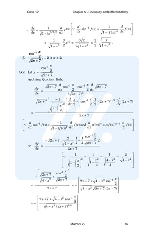
![Differentiate w.r.t. x, the following functions in Exercises 6 to 11.
6. cot–1
1 + sin + 1 – sin
1 + sin – 1 – sin
x x
x x
, 0 < x <
2
π
.
Sol. Let y = cot–1
1 sin 1 sin
1 sin 1 sin
x x
x x
+ + −
+ − −
...(i), 0 < x <
2
π
Let us simplify the given inverse T-function
Now 1 sin x
+ =
2 2
cos sin 2 sin cos
2 2 2 2
x x x x
+ +
=
2
cos sin
2 2
x x
+
= cos
2
x
+ sin
2
x
...(ii)
Again 1 sin x
− =
2 2
cos sin 2 sin cos
2 2 2 2
x x x x
+ −
=
2
cos sin
2 2
x x
−
= cos
2
x
– sin
2
x
...(iii)
(Given: 0 < x <
2
π
. Dividing by 2, 0 <
2
x
<
4
π
and therefore
cos
2
x
> sin
2
x
⇒ cos
2
x
– sin
2
x
> 0)
Putting values from (ii) and (iii) in (i), we have
y = cot–1
cos sin cos sin
2 2 2 2
cos sin cos sin
2 2 2 2
x x x x
x x x x
+ + −
+ − +
= cot–1
2 cos
2
2 sin
2
x
x
= cot–1 cot
2
x
=
2
x
∴
dy
dx
=
1
2
(1) =
1
2
.
7. (log x)log x
, x > 1.
Sol. Let y = (log x)log x
, x > 1 ...(i) [Form ( f (x)) g(x)
]
Taking logs of both sides of (i), we have
log y = log (log x)log x
= log x log (log x) [.
.
. log mn
= n log m]
Differentiating both sides w.r.t. x, we have
d
dx
(log y) =
d
dx
(log x log (log x))
∴
1
y
dy
dx
= log x
d
dx
log (log x) + log (log x)
d
dx
log x
(By Product Rule)
Class 12 Chapter 5 - Continuity and Differentiability
MathonGo 76](https://image.slidesharecdn.com/mathongo-240517043450-33509c08/85/mathongo-com-NCERT-Solutions-Class-12-Maths-Chapter-5-Continuity-and-Differentiability-pdf-76-320.jpg)
![⇒
1
y
dy
dx
= log x .
1
log x
d
dx
log x + log (log x) .
1
x
1
log ( ) ( )
( )
d d
f x f x
dx f x dx
=
∵
⇒
1
y
dy
dx
=
1
x
+
log (log )
x
x
=
1 log (log )
x
x
+
∴
dy
dx
= y
1 log (log )
x
x
+
Putting the value of y from (i),
dy
dx
= (log x)log x
1 log (log )
x
x
+
.
8. cos (a cos x + b sin x) for some constants a and b.
Sol. Let y = cos (a cos x + b sin x) for some constants a and b.
∴
dy
dx
= – sin (a cos x + b sin x)
d
dx
(a cos x + b sin x)
cos ( ) sin ( ) ( )
d d
f x f x f x
dx dx
= −
∵
= – sin (a cos x + b sin x) [– a sin x + b cos x]
= – (– a sin x + b cos x) sin (a cos x + b sin x)
= (a sin x – b cos x) sin (a cos x + b sin x).
9. (sin x – cos x)sin x – cos x
,
4
π
< x <
3
4
π
.
Sol. Let y = (sin x – cos x)sin x – cos x
...(i) [Form ( f (x))g(x)
]
Taking logs of both sides of (i), we have
log y = log (sin x – cos x)(sin x – cos x)
= (sin x – cos x) log (sin x – cos x) [... log mn
= n log m]
Differentiating both sides w.r.t. x, we have
d
dx
log y = (sin x – cos x)
d
dx
log (sin x – cos x)
+ log (sin x – cos x) .
d
dx
(sin x – cos x)
(By Applying Product Rule on R.H. Side)
⇒
1
y
dy
dx
= (sin x – cos x)
1
(sin cos )
x x
−
d
dx
(sin x – cos x)
+ log (sin x – cos x) . (cos x + sin x)
1
log ( ) ( )
( )
d d
f x f x
dx f x dx
=
∵
= (cos x + sin x) + (cos x + sin x) log (sin x – cos x)
⇒
1
y
dy
dx
= (cos x + sin x) [1 + log (sin x – cos x)]
Class 12 Chapter 5 - Continuity and Differentiability
MathonGo 77](https://image.slidesharecdn.com/mathongo-240517043450-33509c08/85/mathongo-com-NCERT-Solutions-Class-12-Maths-Chapter-5-Continuity-and-Differentiability-pdf-77-320.jpg)
![⇒
dy
dx
= y (cos x + sin x) [1 + log (sin x – cos x)]
Putting the value of y from (i),
dy
dx
= (sin x – cos x)(sin x – cos x)
(cos x + sin x) [1 + log (sin x – cos x)]
10. xx
+ xa
+ ax
+ aa
, for some fixed a > 0 and x > 0.
Sol. Let y = xx
+ xa
+ ax
+ aa
∴
dy
dx
=
d
dx
xx
+
d
dx
xa
+
d
dx
ax
+
d
dx
aa
=
d
dx
xx
+ a xa – 1
+ ax
log a + 0 ...(i)
[... aa
is constant as 33
= 27 is constant]
To find
d
dx
(xx
): Let u = xx
...(ii) ( f (x))g(x)
]
∴ Taking logs on both sides of eqn. (ii), we have
log u = log xx
= x log x
∴
d
dx
log u =
d
dx
(x log x)
⇒
1
u
du
dx
= x
d
dx
(log x) + log x
d
dx
x (Product Rule)
= x .
1
x
+ log x . 1 = 1 + log x
⇒
du
dx
= u (1 + log x)
Putting the value of u from (ii),
d
dx
xx
= xx
(1 + log x)
Putting this value in eqn. (i),
dy
dx
= xx
(1 + log x) + a xa – 1
+ ax
log a.
11.
2
– 3
x
x +
2
( – 3)x
x for x > 3.
Sol. Let y =
2
3
x
x −
+
2
( 3)x
x − for x > 3
(Caution. For types ( f (x)) g(x)
± (l(x))m(x)
or ( f (x)) g(x)
± l(x)
or ( f (x))g(x)
± k where k is a constant,
Never begin by taking logs of both sides as
log (m ± n) ≠ log m ± log n)
Put u =
2
3
x
x − and v =
2
( 3)x
x − ∴ y = u + v
∴
dy
dx
=
du
dx
+
dv
dx
...(i)
Now u =
2
( 3)
x
x −
[Type ( f (x))g(x)
]
∴ Taking logs of both sides, we have
Class 12 Chapter 5 - Continuity and Differentiability
MathonGo 78](https://image.slidesharecdn.com/mathongo-240517043450-33509c08/85/mathongo-com-NCERT-Solutions-Class-12-Maths-Chapter-5-Continuity-and-Differentiability-pdf-78-320.jpg)
![log u = log
2
( 3)
x
x −
= (x2
– 3) log x [... log mn
= n log m]
Differentiating both sides w.r.t. x, we have
1
u
du
dx
= (x2
– 3)
d
dx
log x + log x
d
dx
(x2
– 3)
= (x2
– 3)
1
x
+ log x . (2x – 0)
⇒
1
u
du
dx
=
2
3
x
x
−
+ 2x log x ∴
du
dx
= u
2
3
2 log
x
x x
x
−
+
Putting u =
2
( 3)
x
x −
,
du
dx
=
2
( 3)
x
x −
2
3
2 log
x
x x
x
−
+
...(ii)
Again v =
2
( 3)x
x − [( f (x))g(x)
]
∴ Taking logs of both sides, we have
log v = log
2
( 3)x
x − = x2
log (x – 3) [... log mn
= n log m]
∴
d
dx
log v =
d
dx
(x2
log (x – 3))
⇒
1
v
dv
dx
= x2 d
dx
log (x – 3) + log (x – 3)
d
dx
x2
= x2 1
3
x −
d
dx
(x – 3) + log (x – 3) . 2x
⇒
1
v
dv
dx
=
2
3
x
x −
+ 2x log (x – 3)
⇒
dv
dx
= v
2
2 log ( 3)
3
x
x x
x
+ −
−
Putting v =
2
( 3)x
x − ,
dv
dx
=
2
( 3)x
x −
2
2 log ( 3)
3
x
x x
x
+ −
−
...(iii)
Putting values of
du
dx
and
dv
dx
from (ii) and (iii) in (i), we have
dy
dx
=
2
( 3)
x
x −
2
3
2 log
x
x x
x
−
+
+
2
( 3)x
x −
2
2 log ( 3)
3
x
x x
x
+ −
−
.
12. Find
dy
dx
if y = 12(1 – cos t) and x = 10(t – sin t),
–
2
π
< t <
2
π
.
Sol. Given: y = 12(1 – cos t) and x = 10(t – sin t)
Differentiating both equations w.r.t. t, we have
Class 12 Chapter 5 - Continuity and Differentiability
MathonGo 79](https://image.slidesharecdn.com/mathongo-240517043450-33509c08/85/mathongo-com-NCERT-Solutions-Class-12-Maths-Chapter-5-Continuity-and-Differentiability-pdf-79-320.jpg)

![o
r (x – y) (x + y) = – xy (x – y)
Dividing both sides by (x – y) ≠ 0 (... x ≠ y)
x + y = – xy or y + xy = – x
⇒ y(1 + x) = – x ∴ y = –
1
x
x
+
Differentiating both sides w.r.t. x, we have
dy
dx
= – 2
(1 ) ( ) (1 )
(1 )
d d
x x x x
dx dx
x
+ − +
+
= – 2
(1 ) . 1 . 1
(1 )
x x
x
+ −
+
= – 2
1
(1 )
x
+
.
15. If (x – a)2
+ ( y – b)2
= c2
, for some c > 0, prove that
3/2
2
2
2
1 +
dy
dx
d y
dx
is a constant independent of a and b.
Sol. The given equation is (x – a)2
+ ( y – b)2
= c2
...(i)
Differentiating both sides of eqn. (i) w.r.t. x,
2(x – a) + 2(y – b)
dy
dx
= 0
or 2( y – b)
dy
dx
= – 2(x – a) ∴
dy
dx
= –
x a
y b
−
−
...(ii)
Again differentiating both sides of (ii) w.r.t. x,
2
2
d y
dx
= 2
( ) . 1 ( )
( )
dy
y b x a
dx
y b
− − − −
−
Putting the value of
dy
dx
from (i),
2
2
d y
dx
= 2
( )
( ) ( )
( )
x a
y b x a
y b
y b
− −
− − − −
−
−
=
2
2
( )
( )
( )
x a
y b
y b
y b
−
− − +
−
−
=
2 2
3
[( ) ( ) ]
( )
y b x a
y b
− − + −
−
=
2
3
( )
c
y b
−
−
[By (i)] ...(iii)
Putting values of
dy
dx
and
2
2
d y
dx
from (ii) and (iii) in the given
expression
Class 12 Chapter 5 - Continuity and Differentiability
MathonGo 81](https://image.slidesharecdn.com/mathongo-240517043450-33509c08/85/mathongo-com-NCERT-Solutions-Class-12-Maths-Chapter-5-Continuity-and-Differentiability-pdf-81-320.jpg)
![3/2
2
2
2
1
dy
dx
d y
dx
+
, it is =
3/2
2
2
2
3
( )
1
( )
( )
x a
y b
c
y b
−
+
−
−
−
=
2 2 3/2
3
[( ) ( ) ]
( )
y b x a
y b
− + −
−
×
3
2
( )
y b
c
−
−
[... (( y – b)2
)3/2
= ( y – b)3
]
Putting (x – a)2
+ (y – b)2
= c2
from (i)
=
2 3/2
2
( )
c
c
−
=
3
2
c
c
−
= – c
which is a constant and is independent of a and b.
16. If cos y = x cos (a + y) with cos a ≠
≠
≠
≠
≠ ±
±
±
±
± 1, prove that
dy
dx
=
2
cos ( + )
sin
a y
a
.
Sol. Given: cos y = x cos (a + y)
∴ x =
cos
cos ( )
y
a y
+
...(i)
(We have found the value of x because x is not present in the required
value of
dy
dx
)
Differentiating both sides of (i) w.r.t. y,
dx
dy
=
d
dy
cos
cos ( )
y
a y
+
Applying Quotient Rule,
dx
dy
= 2
cos ( ) cos cos cos ( )
cos ( )
d d
a y y y a y
dy dy
a y
+ − +
+
or
dx
dy
= 2
cos ( ) ( sin ) cos ( sin ( ))
cos ( )
a y y y a y
a y
+ − − − +
+
d
dy
∵ cos (a + y) = – sin (a + y)
d
dy
(a + y)
= – sin (a + y) (0 + 1) = – sin (a + y)
or
dx
dy
= 2
cos ( ) sin sin ( ) cos
cos ( )
a y y a y y
a y
− + + +
+
= 2
sin ( ) cos cos ( ) sin
cos ( )
a y y a y y
a y
+ − +
+
= 2
sin ( )
cos ( )
a y y
a y
+ −
+
= 2
sin
cos ( )
a
a y
+
[... sin A cos B – cos A sin B = sin (A – B)]
Class 12 Chapter 5 - Continuity and Differentiability
MathonGo 82](https://image.slidesharecdn.com/mathongo-240517043450-33509c08/85/mathongo-com-NCERT-Solutions-Class-12-Maths-Chapter-5-Continuity-and-Differentiability-pdf-82-320.jpg)
![Taking reciprocals
dy
dx
=
2
cos ( )
sin
a y
a
+
.
17. If x = a (cos t + t sin t) and y = a (sin t – t cos t), find
2
2
d y
dx
.
Sol. Given: x = a (cos t + t sin t) and y = a (sin t – t cos t)
Differentiating both eqns. w.r.t. t, we have
dx
dt
= a sin sin
d
t t t
dt
− +
and
dy
dt
= a cos ( cos )
d
t t t
dt
−
= a sin sin sin
d d
t t t t t
dt dt
− + +
and
dy
dt
= a cos (cos ) cos ( )
d d
t t t t t
dt dt
− +
⇒
dx
dt
= a (– sin t + t cos t + sin t)
and
dy
dt
= a (cos t – (– t sin t + cos t))
⇒
dx
dt
= at cos t ...(i)
and
dy
dt
= a(cos t + t sin t – cos t) = at sin t
We know that
dy
dx
=
/
/
dy dt
dx dt
=
sin
cos
at t
at t
=
sin
cos
t
t
= tan t
Now differentiating both sides w.r.t. x, we have
2
2
d y
dx
=
d
dx
(tan t) = sec2
t
d
dx
(t) → Note
= sec2
t
dt
dx
= sec2
t
1
cos
at t
(By (i))
= sec2
t .
sec t
at
=
3
sec t
at
.
18. If f (x) = |
||
|| x |
||
||3
, show that f ′′
′′
′′
′′
′′(x) exists for all real x and
find it.
Sol. Given: f (x) = | x |3
= x3
if x ≥ 0 ...(i) [... | x | = x if x ≥ 0]
and f (x) = | x |3
= (– x)3
= – x3
if x < 0 ...(ii)
[... | x | = – x if x < 0]
Differentiating both eqns. (i) and (ii) w.r.t. x,
f ′(x) = 3x2
if x > 0 and f ′(x) = – 3x2
if x < 0 ...(iii)
(At x = 0, we can’t write the value of f ′(x) by usual rule of
derivatives because x = 0 is a partitioning point of values of f (x)
given by (i) and (ii)
Class 12 Chapter 5 - Continuity and Differentiability
MathonGo 83](https://image.slidesharecdn.com/mathongo-240517043450-33509c08/85/mathongo-com-NCERT-Solutions-Class-12-Maths-Chapter-5-Continuity-and-Differentiability-pdf-83-320.jpg)
![∴ f ′′(x) = 6x if x > 0 and = – 6x if x < 0 ...(iv)
∴ From (iv), f ′′(x) exists for all x > 0 and for all x < 0
i.e., for all x ∈ R except at x = 0 ...(v)
Let us discuss derivability of f (x) at x = 0
Lf ′(0) =
0
lim
x −
→
( ) (0)
0
f x f
x
−
−
=
0
lim
x −
→
3
0
x
x
− −
[By (ii) and (i)]
=
0
lim
x −
→
– x2
= 0 (On putting x = 0)
Rf ′(0) =
0
lim
x +
→
( ) (0)
0
f x f
x
−
−
=
0
lim
x +
→
3
0
0
x
x
−
−
[By (i)]
=
0
lim
x +
→
x2
= 0 (On putting x = 0)
∴ Lf ′(0) = Rf ′(0) = 0
∴ f (x) is derivable at x = 0 and f ′(0) = 0 ...(vi)
Let us discuss derivability of f ′
′
′
′
′(x) at x = 0
Lf ′′(0) =
0
lim
x −
→
( ) (0)
0
f x f
x
′ ′
−
−
=
0
lim
x −
→
2
3 0
x
x
− −
(By (iii) and (vi))
=
0
lim
x −
→
(– 3x) = – 3(0) = 0 (On putting x = 0)
Rf ′′(0) =
0
lim
x +
→
( ) (0)
0
f x f
x
′ ′
−
−
=
0
lim
x +
→
2
3 0
x
x
−
(By (iii) and (vi))
=
0
lim
x +
→
3x = 3(0) = 0 (On putting x = 0)
∴ Lf ′′(0) = Rf ′′(0) = 0
∴ f ′(x) is derivable at x = 0 and f ′′(0) = 0 ...(vii)
From (iv) and (vii), f ′′(x) exists for all real x and f ′′(x) = 6x if
x > 0 and = – 6x if x < 0 and f ′′(0) = 0.
19. Using mathematical induction, prove that
d
dx
(xn
) = nxn – 1
for all positive integers n.
Sol. Let P(n):
d
dx
(xn
) = nxn – 1
then P(1):
d
dx
(x1
) = 1x0
or
d
dx
(x) = 1 which is true.
⇒ P(1) is true.
Assume P(k) is true. i.e., let
d
dx
(xk
) = kxk – 1
...(i)
Now
d
dx
(xk + 1
) =
d
dx
(xk
. x) =
d
dx
(xk
) . x + xk
.
d
dx
(x)
( )
d du dv
uv v u
dx dx dx
= +
∵
= kxk – 1
. x + xk
. 1 [Using (i)]
Class 12 Chapter 5 - Continuity and Differentiability
MathonGo 84](https://image.slidesharecdn.com/mathongo-240517043450-33509c08/85/mathongo-com-NCERT-Solutions-Class-12-Maths-Chapter-5-Continuity-and-Differentiability-pdf-84-320.jpg)
![= kxk
+ xk
= (k + 1) xk
⇒ P(k + 1) is true.
Hence by P.M.I., the statement is true for all positive integers n.
20. Using the fact that sin (A + B) = sin A cos B + cos A sin B
and the differentiation, obtain the sum formula for cosines.
Sol. Given. sin (A + B) = sin A cos B + cos A sin B
Assuming A and B are functions of x and differentiating both
sides w.r.t. x, we have
cos (A + B) .
d
dx
(A + B) = (sin A) . cos B + sin A . (cos B)
d d
dx dx
+ (cos A) . sin B + cos A . (sin B)
d d
dx dx
⇒ cos (A + B)
A B
d d
dx dx
+
= cos A .
A
d
dx
. cos B +
sin A (– sin B)
B
d
dx
– sin A
A
d
dx
. sin B + cos A . cos B
B
d
dx
= (cos A cos B – sin A sin B)
A
d
dx
+ (cos A cos B – sin A sin B)
B
d
dx
or cos (A + B)
A B
d d
dx dx
+
= (cos A cos B – sin A sin B)
A B
d d
dx dx
+
Dividing both sides by
A
d
dx
+
B
d
dx
, we have
cos (A + B) = cos A cos B – sin A sin B
which is the sum formula for cosines.
21. Does there exist a function which is continuous everywhere
but not differentiable at exactly two points?
Sol. Yes, there exist such function(s).
For example, let us take f (x) = | x – 1 | + | x – 2 | ...(i)
Let us put each expression within modulus equal to 0 i.e.,
x – 1 = 0 and x – 2 = 0 i.e., x = 1 and x = 2.
These two real numbers x = 1 and x = 2 divide the whole real
line (– ∞, ∞) into three sub-intervals (– ∞, 1], [1, 2] and [2, ∞).
In (– ∞, 1] i.e., For x ≤
≤
≤
≤
≤ 1, x – 1 ≤ 0 and x – 2 ≤ 0 and
therefore | x – 1 | = – (x – 1) and | x – 2 | = – (x – 2)
∴ From (i), f (x) = – (x – 1) – (x – 2)
= – x + 1 – x + 2 = 3 – 2x for x ≤ 1 ...(ii)
In [1, 2] i.e., for 1 ≤ x ≤ 2, x – 1 ≥ 0 and x – 2 ≤ 0 and
– ∞ 1 2 ∞
Class 12 Chapter 5 - Continuity and Differentiability
MathonGo 85](https://image.slidesharecdn.com/mathongo-240517043450-33509c08/85/mathongo-com-NCERT-Solutions-Class-12-Maths-Chapter-5-Continuity-and-Differentiability-pdf-85-320.jpg)
![therefore | x – 1 | = x – 1 and | x – 2 | = – (x – 2).
From (i), f (x) = x – 1 – (x – 2) = x – 1 – x + 2 = 1 for
1 ≤ x ≤ 2 ...(iii)
Again in [2, ∞) i.e., for x ≥ 2, x – 1 ≥ 0 and x – 2 ≥ 0 and
therefore
| x – 1 | = x – 1 and | x – 2 | = x – 2.
∴ From (i) f (x) = x – 1 + x – 2 = 2x – 3 for x ≥ 2 ...(iv)
Hence function (i) given in modulus form can be expressed as
piece-wise function given by (ii), (iii) and (iv)
i.e., f (x) = 3 – 2x for x ≤ 1 ...(ii)
= 1 for 1 ≤ x ≤ 2 ...(iii)
= 2x – 3 for x ≥ 2 ...(iv)
Now the three values of f (x) given by (ii), (iii) and (iv) are
polynomial functions and constant function and hence are
continuous and derivable for all real values of x except possibly at
the partitioning points x = 1 and x = 2. ...(v)
To examine continuity at x = 1
Left Hand limit = –
1
lim
x →
f (x) =
–
1
lim
x →
(3 – 2x) [By (ii)]
Put x = 1; = 3 – 2 = 1
Right Hand Limit =
1
lim
x +
→
f (x) =
1
lim
x +
→
1 [By (iii)]
Put x = 1; = 1
∴
–
1
lim
x →
f (x) =
1
lim
x +
→
f (x) (= 1)
∴
1
lim
x →
f (x) exists and = 1 = f (1) (... From (iii) f (1) = 1]
∴ f (x) is continuous at x = 1 ...(vi)
To examine derivability at x = 1
Left Hand derivative = Lf ′(1) = –
1
lim
x →
( ) (1)
1
f x f
x
−
−
= –
1
lim
x →
3 2 1
1
x
x
− −
−
[By (ii) and f (1) = 1 (proved above)]
=
–
1
lim
x →
2 2
1
x
x
− +
−
= –
1
lim
x →
2( 1)
1
x
x
− −
−
= –
1
lim
x →
(– 2) = – 2
Right Hand derivative = Rf ′(1) =
1
lim
x +
→
( ) (1)
1
f x f
x
−
−
=
1
lim
x +
→
1 1
1
x
−
−
(By (iii))
=
1
lim
x +
→
0
1
x −
=
1
lim
x +
→
0
Non-zero
[x → 1+
⇒ x > 1 ⇒ x – 1 > 0 ⇒ x – 1 ≠ 0]
Class 12 Chapter 5 - Continuity and Differentiability
MathonGo 86](https://image.slidesharecdn.com/mathongo-240517043450-33509c08/85/mathongo-com-NCERT-Solutions-Class-12-Maths-Chapter-5-Continuity-and-Differentiability-pdf-86-320.jpg)
![=
1
lim
x +
→
0 = 0
∴ Lf ′(1) ≠ Rf ′(1
∴ f (x) is not differentiable at x = 1 ...(vii)
To examine continuity at x = 2
Left hand limit =
2
lim
x −
→
f (x) =
2
lim
x −
→
1 (By (ii)) = 1
Right Hand Limit =
2
lim
x +
→
f (x) =
2
lim
x +
→
(2x – 3) [By (iv)]
Putting x = 2, = 4 – 3 = 1
∴
2
lim
x −
→
f (x) =
2
lim
x +
→
f (x) (= 1)
∴
2
lim
x →
f (x) exists and = 1 = f (2) [... From (iii), f (2) = 1]
∴ f (x) is continuous at x = 2 ...(viii)
To examine derivability at x = 2
Lf ′(2) =
2
lim
x −
→
( ) (2)
2
f x f
x
−
−
=
2
lim
x −
→
1 1
2
x
−
−
(By (iii))
=
2
lim
x −
→
0
Non-zero
[... x → 2–
⇒ x < 2 ⇒ x – 2 < 0 ⇒ x – 2 ≠ 0]
=
2
lim
x −
→
0 = 0
Rf ′(2) =
2
lim
x +
→
( ) (2)
2
f x f
x
−
−
=
2
lim
x +
→
2 3 1
2
x
x
− −
−
[By (iv)]
=
2
lim
x +
→
2 4
2
x
x
−
−
=
2
lim
x +
→
2( 2)
2
x
x
−
−
=
2
lim
x +
→
2 = 2
∴ Lf ′(2) ≠ Rf ′(2)
∴ f (x) is not differentiable at x = 2 ...(ix)
From (v), (vi) and (viii), we can say that f (x) is continuous for
all real values of x i.e., continuous everywhere.
From (v), (vii) and (ix), we can say that f (x) is not
differentiable at exactly two points x = 1 and x = 2 on the real
line.
22. If y =
f (x) g(x) h(x)
l m n
a b c
, prove that
dy
dx
=
′ ′ ′
f (x) g (x) h (x)
l m n
a b c
.
Sol. Given: y =
( ) ( ) ( )
f x g x h x
l m n
a b c
Class 12 Chapter 5 - Continuity and Differentiability
MathonGo 87](https://image.slidesharecdn.com/mathongo-240517043450-33509c08/85/mathongo-com-NCERT-Solutions-Class-12-Maths-Chapter-5-Continuity-and-Differentiability-pdf-87-320.jpg)
![Expanding the determinant along first row,
y = f (x) (mc – nb) – g(x) (lc – na) + h(x) (lb – ma)
∴
dy
dx
= (mc – nb)
d
dx
f (x) – (lc – na)
d
dx
g(x)
+ (lb – ma)
d
dx
h(x)
= (mc – nb) f ′(x) – (lc – na) g ′(x) + (lb – ma) h′(x) ...(i)
R.H.S. =
( ) ( ) ( )
f x g x h x
l m n
a b c
′ ′ ′
Expanding along first row,
= f ′(x) (mc – nb) – g′(x) (lc – na) + h′(x) (lb – ma)
= (mc – nb) f ′(x) – (lc – na) g′(x) + (lb – ma) h′(x) ...(ii)
From (i) and (ii), we have L.H.S. = R.H.S.
23. If y =
–1
cos
a x
e , – 1 ≤
≤
≤
≤
≤ x ≤
≤
≤
≤
≤ 1, show that
(1 – x2
)
2
2
d y
dx
– x
dy
dx
– a2
y = 0.
Sol. Given: y =
–1
cos
a x
e ...(i)
∴
dy
dx
=
–1
cos
a x
e
d
dx
(a cos–1
x)
( ) ( )
( )
f x f x
d d
e e f x
dx dx
=
∵
or
dy
dx
=
–1
cos
a x
e . a
2
1
1 x
−
−
=
1
cos
2
1
a x
ae
x
−
−
−
Cross-multiplying, 2
1 x
−
dy
dx
= – a
–1
cos
a x
e = – ay
(By (i)) ...(ii)
Again differentiating both sides w.r.t. x,
2
1 x
−
d
dx
dy
dx
+
dy
dx
d
dx
(1 – x2
)1/2
= – a
dy
dx
⇒
2
1 x
−
2
2
d y
dx
+
dy
dx
1
2
(1 – x2
)–1/2 d
dx
(1 – x2
) = – a
dy
dx
⇒ 2
1 x
−
2
2
d y
dx
+
1
2
dy
dx 2
1
1 x
−
(– 2x) = – a
dy
dx
Multiplying by L.C.M. = 2
1 x
− ,
(1 – x2
)
2
2
d y
dx
– x
dy
dx
= – a 2
1 x
−
dy
dx
= – a (– ay) [By (ii)]
= a2
y
⇒ (1 – x2
)
2
2
d y
dx
– x
dy
dx
– a2
y = 0.
Class 12 Chapter 5 - Continuity and Differentiability
MathonGo 88](https://image.slidesharecdn.com/mathongo-240517043450-33509c08/85/mathongo-com-NCERT-Solutions-Class-12-Maths-Chapter-5-Continuity-and-Differentiability-pdf-88-320.jpg)