Mathematics
Author
TNAU, Tamil Nadu
Index
SN Lecture Page No
1 Three dimensional Analytical geometry 5-10
2 Analytical geometry 11-18
3 Binomial theorem 19-21
4 Conics 22-25
5 Differentiation 26-29
6 Chain rule differentiation 30-40
7 Differential equations 41-43
8 Circles 44-45
9 Chain rule differentiation 46-56
10 Integration 57-62
11 Inverse of a matrix 63-68
12 Matrices 69-80
13 Physical and economic optimum for single input 81-89
14 Model 90-100
15 Chain rule differentiation 101-111
16 Permutation and combination 112-116
17 Physical and Economic Optimum for single input 117
18 Population dynamics 118-122
19 Progressions 123-128
20
Second order differential equations with constant
coefficients
129-130
21 Inverse of a matrix 131-132
22 Demand function and supply functions 133-137
23 Vector algebra 138-143
Three dimensional Analytical geometry
Let OX ,OY & OZ be mutually perpendicular straight lines meeting at a point O. The
extension of these lines OX1
, OY1
and OZ1
divide the space at O into octants(eight). Here
mutually perpendicular lines are called X, Y and Z co-ordinates axes and O is the origin. The
point P (x, y, z) lies in space where x, y and z are called x, y and z coordinates respectively.
Z
P(x,y,z)
Y
O
x R
z
x
M
y N
X
where NR = x coordinate, MN = y coordinate and PN = z coordinate
Mathematics
www.AgriMoon.Com
5
Distance between two points
The distance between two points A(x1, y1, z1) and B(x2, y2,z2) is
dist AB = ( ) ( ) ( )2
1
2
2
1
2
2
1
2 z
z
y
y
x
x −
+
−
+
−
In particular the distance between the origin O (0,0,0) and a point P(x,y,z) is
OP = 2
2
2
z
y
x +
+
The internal and External section
Suppose P(x1, y1, z1) and Q(x2, y2,z2) are two points in three dimensions.
P(x1,y1,z1) A(x, y, z) Q(x2, y2,z2)
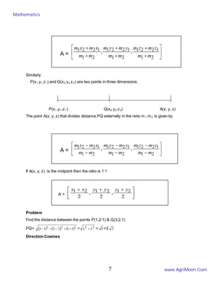
The point A(x, y, z) that divides distance PQ internally in the ratio m1:m2 is given by
Mathematics
www.AgriMoon.Com
6
A = 





+
+
+
+
+
+
2
1
1
2
2
1
2
1
1
2
2
1
2
1
1
2
2
1 ,
,
m
m
z
m
z
m
m
m
y
m
y
m
m
m
x
m
x
m
Similarly
P(x1, y1, z1) and Q(x2, y2,z2) are two points in three dimensions.
P(x1,y1,z1) Q(x2, y2, z2) A(x, y, z)
The point A(x, y, z) that divides distance PQ externally in the ratio m1:m2 is given by
A = 





−
−
−
−
−
−
2
1
1
2
2
1
2
1
1
2
2
1
2
1
1
2
2
1 ,
,
m
m
z
m
z
m
m
m
y
m
y
m
m
m
x
m
x
m
If A(x, y, z) is the midpoint then the ratio is 1:1
A = 




 +
+
+
2
,
2
,
2
2
1
2
1
2
1 z
z
y
y
x
x
Problem
Find the distance between the points P(1,2-1) & Q(3,2,1)
PQ= ( ) ( ) ( )2
2
2 1
1
2
2
1
3 +
+
−
+
− = 2
2 2
2 + = 8 =2 2
Direction Cosines
Mathematics
www.AgriMoon.Com
7
P(x,y,z)
M
O
γ
α
β
y
z
x
Let P(x, y, z) be any point and OP = r. Let α,β,γ be the angle made by line OP with OX, OY
& OZ. Then α,β,γ are called the direction angles of the line OP. cos α, cos β, cos γ are called
the direction cosines (or dc’s) of the line OP and are denoted by the symbols I, m ,n.
Result
By projecting OP on OY, PM is perpendicular to y axis and the β
=
∠POM also OM = y
r
y
=
∴ β
cos
Similarly,
r
x
=
α
cos
r
z
=
γ
cos
(i.e) l = ,
r
x
m = ,
r
y
n =
r
z
∴l2
+ m2
+ n2
=
2
2
2
2
r
z
y
x +
+
( ⇒
+
+
= 2
2
2 z
y
x
r
 Distance from the origin)
∴ l2
+ m2
+ n2
= 1
2
2
2
2
2
2
=
+
+
+
+
z
y
x
z
y
x
l2
+ m2
+ n2
= 1
(or) cos2
α + cos2
β + cos2
γ = 1.
Note :-
The direction cosines of the x axis are (1,0,0)
Mathematics
www.AgriMoon.Com
8
The direction cosines of the y axis are (0,1,0)
The direction cosines of the z axis are (0,0,1)
Direction ratios
Any quantities, which are proportional to the direction cosines of a line, are called
direction ratios of that line. Direction ratios are denoted by a, b, c.
If l, m, n are direction cosines an a, b, c are direction ratios then
a ∝ l, b ∝ m, c ∝ n
(ie) a = kl, b = km, c = kn
(ie) k
n
c
m
b
l
a
=
=
= (Constant)
(or)
k
c
n
b
m
a
l 1
=
=
= (Constant)
To find direction cosines if direction ratios are given
If a, b, c are the direction ratios then direction cosines are
⇒
=
k
a
l 1
l =
k
a
similarly m =
k
b
(1)
n =
k
c
l2
+m2
+n2
= )
(
1 2
2
2
2
c
b
a
k
+
+
(ie) 1 = )
(
1 2
2
2
2
c
b
a
k
+
+
2
2
2
2 c
b
a
k +
+
=
⇒
Taking square root on both sides
K = 2
2
2
c
b
a +
+
∴
2
2
2
2
2
2
2
2
2
,
,
c
b
a
c
n
c
b
a
b
m
c
b
a
a
l
+
+
=
+
+
=
+
+
=
Mathematics
www.AgriMoon.Com
9
o
Problem
1. Find the direction cosines of the line joining the point (2,3,6) & the origin.
Solution
By the distance formula
7
49
36
9
4
6
3
2 2
2
2
2
2
2 =
=
+
+
=
+
+
=
+
+
= z
y
x
r
Direction Cosines are r
l = cos ∝ =
7
2
=
r
x
m = cos β =
7
3
=
r
y
n = cos γ =
7
6
=
r
z
2. Direction ratios of a line are 3,4,12. Find direction cosines
Solution
Direction ratios are 3,4,12
(ie) a = 3, b = 4, c = 12
Direction cosines are
l =
13
3
169
3
12
4
3
3
2
2
2
2
2
2
=
=
+
+
=
+
+ c
b
a
a
m= 13
4
169
4
12
4
3
4
2
2
2
2
2
2
=
=
+
+
=
+
+ c
b
a
b
n= 13
12
169
12
12
4
3
12
2
2
2
2
2
2
=
=
+
+
=
+
+ c
b
a
c
Note
1) The direction ratios of the line joining the two points A(x1, y1, z1) &
B (x2, y2, z2) are (x2 – x1, y2 – y1, z2 – z1)
2) The direction cosines of the line joining two points A (x1, y1, z1) &
B (x2, y2, z2) are
r
z
z
r
y
y
r
x
x 1
2
1
2
1
2 ,
,
−
−
−
r = distance between AB.
y
z
(2,3,6)
x
Mathematics
www.AgriMoon.Com
10
Analytical geometry
Introduction
The branch of mathematics where algebraic methods are employed for solving
problems in geometry is known as analytical geometry. It is sometimes called Cartesian
Geometry.
Let X’OX and Y’OY be two perpendicular straight lines intersecting at the point O.
The fixed point O is called origin. The horizontal line X’OX is known as X –axis and the
vertical line Y’OY be Y-axis. These two axes divide the entire plane into four parts known
as Quadrants.
Y
P′(-X,Y) P(X,Y)
X ′ M O N X
Q′(-X,-Y) Q(X,-Y)
Y ′
All the values right of the origin along the X-axis are positive and all the values
left of the origin along the X- axis are negative. Similarly all the values above the origin
along Y – axis are positive and below the origin are negative.
Let P be any point in the plane. Draw PN perpendicular to X –axis. ON and PN
are called X and Y co-ordinates of P respectively and is written as P (X,Y). In particular
the origin O has co-ordinates (0,0) and any point on the X-axis has its Y co-ordinate as
zero and any point on the Y-axis has its X-co-ordinates as zero.
Straight lines
A straight line is the minimum distance between any two points.
Slope
The slope of the line is the tangent of the angle made by the line with positive
direction of X – axis measured in the anticlockwise direction.
Mathematics
www.AgriMoon.Com
11
A
B
Y
θ
X ′ O X
Y′
let the line AB makes an angle θ with the positive direction of X-axis as in the figure.
The angle θ is called the angle of inclination and tanθ is slope of the line or gradient of
the line. The slope of the line is denoted by m. i.e., slope = m = tanθ
Y Y
θ (obtuse) θ (acute)
X
X
Y ′
Slope = m = tanθ Slope = m= tan θ Slope is negative Slope is positive
Note
(i) The slope of any line parallel to X axis is zero.
(ii) Slope of any line parallel to Y axis is infinity
(iii) The slope of the line joining two points (x1, y1) and (x2, y2) is
Slope = m = tanθ =
2
1
2
1
x
x
y
y
−
−
X ′
Y′
Mathematics
www.AgriMoon.Com
12
o
D
M
A
y -c
B (O, C)
X
XI
Y
(iv) When two or more lines are parallel then their slopes are equal
(v) When two lines are perpendicular then the product of their slopes is –1
i.e., m1m2 = -1
Equation of a straight line
There are several forms of a straight line. They are,
1. Slope – intercept form
Let the given line meet y-axis at B (o, c). We call OB as Y – intercept. Let A be
any point on the given line. Draw AM perpendicular to OX and BD ⊥ AM. Let this line
make an angle θ with X axis. Then the slope,
m = tan θ =
BD
AD
=
OM
DM
AM −
=
OM
OB
AM −
=
x
c
y −
ie. m =
x
c
y −
mx = y – c
y = mx + c
Hence, the equation of a line with slope ‘m’ and y – intercept ‘c’ is given by
y = mx + c
Note:
(i) Any line passing through the origin does not cut y – axis (c = 0) i.e., y –
intercept is zero. Therefore its equation is y = mx
(ii) Any line which is parallel to x – axis has slope equal to zero. Therefore its
equation is y = c (Because m = 0)
(iii) Any line perpendicular to x-axis, ie which is parallel to y-axis at a distance of K
units from the origin is given by x = k.
Example 1: Find the equation of a straight line whose
(i) Slope is four and y intercept is –3
(ii) Inclination is 300
and y intercept is 5
Mathematics
www.AgriMoon.Com
13
Solution: (i) Slope (m) = 4
Y intercept (c) = -3
Equation of a line is y = mx + c
Y = 4x – 3
Equation of a line is 4x – y – 3 = 0
(ii) θ = 300
, y intercept = 5
Slope = tan θ
m = tan 300
=
3
1
Equation of a line is y = mx + c
Y =
3
1
x + 5
3 y = x + 5 3
Equation of a line is x - 3 y +5 3 = 0
Example 2: Calculate the slope and y intercept of the line 2x – 3y + 1= 0
Solution: 2x – 3y + 1 = 0
3y = 2x + 1
y =
3
2x
+
3
1
Comparing with y = mx + c, we get
m =
3
2
, c =
3
1
Slope =
3
2
; y intercept =
3
1
2. Slope – one point form
Let the line AB make an angle θ with x- axis as shown in the figure and pass
through the point P (x1, y1). If (x, y) represents a point other than the point (x1, y1), then
m =
1
1
x
x
y
y
−
−
where m is the slope of the line or y – y1 = m (x – x1).
Hence the equation of a line passing through a point (x1, y1) and having slope ‘m’ is
A
X
P
θ
(x1,y1)
o
Y
B
Mathematics
www.AgriMoon.Com
14
y – y1 = m (x – x1).
Example: Find the equation of a straight line passing through (-4,5) and having slope -
3
2
Solution: Slope = -
3
2
Point (-4,5)
Equation of the line is (y-y1) = m(x-x1)
y – 5 = -
3
2
(x+4)
3y – 15 = -2x –8
∴Equation of a line is 2x + 3y – 7 = 0
3. Two points form
Let P (x1, y1) and Q (x2, y2) be any two points on the given line AB. We know,
the slope, m =
1
2
1
2
x
x
y
y
−
−
.
We have the slope-point form of a line as
y – y1 = m (x – x1).
Substituting the value of m in the above equation we get,
y – y1 =
1
2
1
2
x
x
y
y
−
−
(x – x1).
ie
1
2
1
y
y
y
y
−
−
=
1
2
1
x
x
x
x
−
−
Hence, the equation of a line passing through two points is given by
1
2
1
y
y
y
y
−
−
=
1
2
1
x
x
x
x
−
−
o
A
Q
(x2,y2)
θ
(x1,y1)
P
Y
X
B
Mathematics
www.AgriMoon.Com
15
X
0
A (a, 0)
B (0, b)
Example: Find the equation of the straight line passing through the points (3,6) and (-
2,5).
Solution : Equation of the line is
1
2
1
y
y
y
y
−
−
=
1
2
1
x
x
x
x
−
−
6
5
6
−
−
y
=
3
2
3
−
−
−
x
1
6
−
−
y
=
5
3
−
−
x
5y – 30 = x – 3
x – 5y –3 + 30 = 0
Equation of the line is x – 5y +27 = 0
4. Intercept form
Let AB represent the given line which intersects X – axis at A (a, 0) and Y- axis at
B (0, b). We call OA and OB respectively as x and y intercepts of the line.
The two points form of the equation is given by
1
2
1
y
y
y
y
−
−
=
1
2
1
x
x
x
x
−
−
Substituting (a, 0) for (x1,y1) and (0, b) for (x2, y2), we get the equation as
0
0
−
−
b
y
=
a
a
x
−
−
0
ie
b
y
=
a
a
x
−
−
b
y
=
a
x
−
-
a
a
−
Thus,
b
y
=
a
x
−
+ 1
Mathematics
www.AgriMoon.Com
16
∴
a
x
+
b
y
= 1
Hence, the equation of a line having x-intercept ‘a’ and y-intercept ‘b’ is given by
a
x
+
b
y
= 1
Example: Find the intercepts cut off by the line 2x – 3y + 5 = 0 on the axes.
Solution
x – intercept: put y = 0
∴2x + 5 = 0
x =
2
5
−
This is the x – intercept
y – intercept: Put x = 0
-3y + 5 = 0
∴y =
3
5
This is the y – intercept
Example : Give the mathematical equation of the supply function of a commodity such
that the quantity supplied is zero when the price is Rs.5 or below and it increase
continuously at the constant rate of 10 units for each one rupee rise in price above Rs.5.
Solution
A(0,5) B(10,6) C(20,7)
Point B is (10,6)
Point C is (20,7)
Equation of straight line joining two points is
1
2
1
y
y
y
y
−
−
=
1
2
1
x
x
x
x
−
−
6
7
6
−
−
y
=
10
20
10
−
−
x
1
6
−
y
=
10
10
−
x
10 (y-6) = x –10
10y-60 = x-10
x -10y - 50=0
Mathematics
www.AgriMoon.Com
17
Note
The four equations we have obtained are all first degree equations in x and y. On
the other hand it can be shown that the general first degree equation in x and y always
represents a straight line. Hence we can take general equation of a straight line as ax +
by + c = 0 with at least one of a or b different from c. Further, this gives by = - ax – c
i.e. y =
b
ax
−
-
b
c
Now, comparing this with the equation y = mx + c, we get
slope = m =
b
a
−
= - 





y
of
t
coefficien
x
of
t
coefficien
Mathematics
www.AgriMoon.Com
18
1
BINOMIAL THEOREM
A Binomial is an algebraic expression of two terms which are connected by the operation
‘+’ (or) ‘-‘
For example, x+siny, 3x2
+2x, cosx+sin x etc… are binomials.
Binomial Theorem for positive integer:
If n is a positive integer then
( ) n
n
n
n
r
r
n
r
n
n
n
a
x
nC
a
x
nC
a
x
nC
a
x
nC
a
x
nC
a
x 0
1
1
1
1
1
1
0
0 ...
... +
+
+
+
+
+
=
+ −
−
−
− ----(1)
Some Expansions
a) If we put a = -a in the place of a in
( ) ( ) ( ) ( ) ( ) ( )n
n
n
n
r
r
n
r
n
n
n a
x
nC
a
x
nC
a
x
nC
a
x
nC
a
x
nC
a
x −
+
−
+
+
−
+
+
−
+
−
=
− −
−
−
− 0
1
1
1
1
1
1
0
0 ...
...
( ) ( ) ( ) ( ) n
n
r
n
n
r
r
r
n
r
r
n
n
n
a
x
nC
a
x
nC
a
x
nC
a
x
nC
a
x
nC
a
x 0
1
1
1
1
1
1
0
0 1
...
1
...
1
... −
+
+
−
+
+
−
+
+
−
=
− −
−
−
−
b) Put x =1 and a = x in (1)
( ) n
n
r
r
n
x
nC
x
nC
x
nC
x
nC
x +
+
+
+
+
+
=
+ ...
...
1
1 2
2
1
( ) ( ) ( )( ) n
n x
x
n
n
n
x
n
n
nx
x +
−
−
+
−
+
+
=
+ ......
!
3
2
1
!
2
1
1
1 3
2 ----------(2)
c) Put x = 1 and a = -x in (1)
( ) ( ) ( ) n
n
n
r
r
r
n
x
nC
x
nC
x
nC
x
nC
x 1
...
1
...
1
1 2
2
1 −
+
+
−
+
−
+
−
=
−
( ) ( ) ( )( ) ( ) n
n
n x
x
n
n
n
x
n
n
nx
x 1
......
!
3
2
1
!
2
1
1
1 3
2 −
+
−
−
−
−
+
−
=
− -----------(3)
(d) Replacing n by – n in equation (2)
( ) ( ) ( )( ) ( ) n
n
n x
x
n
n
n
x
n
n
nx
x 1
......
!
3
2
1
!
2
1
1
1 3
2 −
+
+
+
−
+
+
−
=
+ − ---------(4)
e) Replacing n by – n in equation (3)
( ) ( ) ( )( ) n
n x
x
n
n
n
x
n
n
nx
x +
+
+
+
+
+
+
=
− − ......
!
3
2
1
!
2
1
1
1 3
2 -----------(5)
Special Cases
1. ( ) ......
1
1 3
2
1 x
x
x
x −
+
−
=
+ −
2. ( ) ......
1
1 3
2
1 x
x
x
x +
+
+
=
− −
3. ( ) ......
4
3
2
1
1 3
2
2 x
x
x
x −
+
−
=
+ −
4. ( ) ......
4
3
2
1
1 3
2
2 x
x
x
x +
+
+
=
− −
Mathematics
www.AgriMoon.Com
19
2
Note:
1. There are n+1 terms in the expansion of (x+a)n
.
2. In the expansion the general term is r
r
n
r a
x
nC −
. Since this is the (r+1)th
term, it is denoted by
Tr+1 i.e. r
r
n
r
r a
x
nC
T −
+ =
1
.
3. n
r nC
nC
nC
nC
nC ,...
,...
,
, 2
1
0 are called binomial coefficients.
4. From the relation r
n
r nC
nC −
= , we see that the coefficients of terms equidistant from the
beginning and the end are equal.
Note: The number of terms in the expansion of (x+a)n
depends upon the index n. the index is
either even (or) odd. Then the middle term is
Case(i): n is even
The number of terms in the expansion is (n+1), which is odd.
Therefore, there is only one middle term and is given by
1
2
+
n
T
Case(ii) : n is odd
The number of terms in the expansion is (n+1), which is even.
Therefore, there are two middle terms and they are given by
2
1
+
n
T and
2
3
+
n
T
Examples
1. Expand (i)
6
2 1
2 





+
x
x
2. Find 117
.
Solution:
117
= (1+10)7
( ) ( ) ( ) ( ) ( ) ( ) ( ) ( ) ( ) ( )
( ) ( ) ( ) ( ) ( ) ( )7
0
7
6
1
6
5
2
5
4
3
4
3
4
3
2
5
2
1
6
1
0
7
0
10
1
7
10
1
7
10
1
7
10
1
7
10
1
7
10
1
7
10
1
7
10
1
7
C
C
C
C
C
C
C
C
+
+
+
+
+
+
+
=
7
6
5
4
3
2
10
7
6
5
4
3
2
1
1
2
3
4
5
6
7
10
6
5
4
3
2
1
2
3
4
5
6
7
10
5
4
3
2
1
3
4
5
6
7
10
4
3
2
1
4
5
6
7
10
3
2
1
5
6
7
10
2
1
6
7
70
1
×
×
×
×
×
×
×
×
×
×
×
×
+
×
×
×
×
×
×
×
×
×
×
+
×
×
×
×
×
×
×
×
+
×
×
×
×
×
×
+
×
×
×
×
+
×
×
+
+
=
= 1+ 70 + 2100 +35000 + 350000 + 2100000 + 7000000 + 10000000
= 19487171
Mathematics
www.AgriMoon.Com
20
3
2. Find the coefficient of x5
in the expansion of
17
3
1






+
x
x
Solution
In the expansion of
17
3
1






+
x
x , the general term is
r
r
r
r
x
x
C
T 





=
−
+ 3
17
1
1
17
r
r x
C
4
17
17
−
=
Let 1
+
r
T be the term containing x5
then, 17-4r = 5 ⇒ r = 3
∴ 1
+
r
T = 1
3+
T
( )
3
4
17
17
−
= x
Cr
= 680 x5
∴coefficient of x5
= 680.
3. Find the constant term in the expansion of
10
2
2






−
x
x
Solution
In the expansion of
10
2
2






−
x
x , the general term is
( )
r
r
r
r
x
x
C
T 




 −
=
−
+ 2
10
1
2
10
( ) ( )
r
r
r
r
r
r
r
r x
C
x
x
C
2
2
10
2
2
10
2
10
2
10
−
−
−
−
=
−
=
( ) 2
5
10
2
10
r
r
r x
C
−
−
=
Let 1
+
r
T be the Constant term then,
2
5
10 r
−
= 0⇒ r = 2
∴ The constant term ( )
( )
2
2
5
10
2
2 2
10
−
−
= x
C
= 0
4
2
1
9
10
x
×
×
×
×
= 180
Mathematics
www.AgriMoon.Com
21
Conics
Definition
A conic is defined as the locus of a point, which moves such that its distance
from a fixed line to its distance from a fixed point is always constant. The fixed point is
called the focus of the conic. The fixed line is called the directrix of the conic. The
constant ratio is the eccentricity of the conic.
L
M P
F
L is the fixed line – Directrix of the conic.
F is the fixed point – Focus of the conic.
=
PM
FP
constant ratio is called the eccentricity = ‘e’
Classification of conics with respect to eccentricity
1. If e < 1, then the conic is an Ellipse
M1 M2
L2 B L1
A1
A
LI
2 LI
1
BI
M2
1
M1
1
1) The standard equation of an ellipse is 1
2
2
2
2
=
+
b
y
a
x
O
F2
F1
S
SI
Mathematics
www.AgriMoon.Com
22
2) The line segment AA1
is the major axis of the ellipse, AA1
= 2a
3) The equation of the major axis is Y = 0
4) The line segment BB1
is the minor axis of the ellipse, BB1 = 2b
5) The equation of the minor axis is X = 0
6) The length of the major axis is always greater than the minor axis.
7) The point O is the intersection of major and minor axis.
8) The co-ordinates of O are (0,0)
9) The foci of the ellipse are S(ae,0)and SI
(-ae,0)
10) The vertical lines passing through the focus are known as Latusrectum
11) The length of the Latusrectum is
a
b2
2
12) The points A (a,0) and A1
(-a,0)
13) The eccentricity of the ellipse is e =
2
2
1
a
b
−
14) The vertical lines M1 M1
1
and M2 M2
1
are known as the directrix of the ellipse and
their respective
equations are x =
e
a
and x =
e
a
−
2. If e = 1, then the conic is a Parabola.
L
P
O S
L1
Q
1) The Standard equation of the parabola is y2
= 4ax.
2) The horizontal line is the axis of the parabola.
3) The equation of the axis of the parabola is Y = 0
4) The parabola y2
= 4ax is symmetric about the axis of the parabola.
5) The vertex of the parabola is O (0,0)
6) The line PQ is called the directrix of the parabola.
Mathematics
www.AgriMoon.Com
23
7) The equation of the directrix is x = -a
8) The Focus of the parabola is S(a,0).
9) The vertical line passing through S is the latus rectum. LL1
is the Latus rectum and
its length LL1
= 4a
3. If e > 1 ,then the conic is Hyperbola.
B
M2
L1 M1 L2
AI
O A
SI
S
1
L′ M1
1
BI
M2
1
2
L′
1) The standard equation of an hyperbola is 1
2
2
2
2
=
−
b
y
a
x
2) The line segment AA1
is the Transverse axis of the hyperbola ,AA1
= 2a
3) The equation of the Transverse axis is Y = 0
4) The line segment BB1
is the Conjugate axis of the hyperbola ,BB1
= 2b
5) The equation of the Conjugate axis is X = 0
6) The point O is the intersection of Transverse and Conjugate axis.
7) The co-ordinates of O are (0,0)
8) The foci of the hyperbola are S(ae,0)and SI
(-ae,0)
9) The vertical lines passing through the focus are known as Latusrectum
10) The length of the Latusrectum is
a
b2
2
11) The points A (a,0) and A1
(-a,0)
12) The eccentricity of the hyperbola is e =
2
2
1
a
b
+
Mathematics
www.AgriMoon.Com
24
13) The vertical lines M1 M1
1
and M2 M2
1
are known as the directrix of the hyperbola and
their respective equations are x =
e
a
and x =
e
a
−
Mathematics
www.AgriMoon.Com
25
DIFFERENTIATION
In all practical situations we come across a number of variables. The variable is
one which takes different values, whereas a constant takes a fixed value.
Let x be the independent variable. That means x can take any value. Let y be a
variable depending on the value of x. Then y is called the dependent variable. Then y is
said to be a function of x and it is denoted by y = f(x)
For example if x denotes the time and y denotes the plant growth, then we know
that the plant growth depends upon time. In that case, the function y=f(x) represents the
growth function. The rate of change of y with respect to x is denoted by
dx
dy
and called as
the derivative of function y with respect to x.
S.No. Form of Functions y=f(x)
dx
dy
1. Power Formula xn
( ) 1
−
= n
n
nx
dx
x
d
2. Constant C 0
3. Constant with variable Cy
dx
dy
C
4. Exponential ex
ex
5. Constant power x ax
ax
log a
6. Logirthamic logx
x
1
7. Differentiation of a sum y = u + v
where u and v are
functions of x.
( )
dx
dv
dx
du
v
u
dx
d
dx
dy
+
=
+
=
8. Differentiation of a
difference
y = u – v
where u and v are
functions of x.
( )
dx
dv
dx
du
v
u
dx
d
dx
dy
−
=
−
=
9. Product rule of
differentiation
y = uv,
where u and v are
functions of x.
( )
dx
du
v
dx
dv
u
uv
dx
d
dx
dy
+
=
=
10. Quotient rule of
differentiation
y =
v
u
,
2
v
v
u
u
v
v
u
dx
d
dx
dy ′
−
′
=






=
Mathematics
www.AgriMoon.Com
26
where u and v are
functions of x.
where
dx
du
u =
′ ,
dx
dv
v =
′
Example
1. Differentiate each of the following function
Solution
2. Differentiate following function
Solution
Here is the derivative.
3. Differentiate following function
Solution
diff. w.r.to x
4. Differentiate the following functions.
a)
Solution
Mathematics
www.AgriMoon.Com
27
diff y w. r. to x
5. Differentiate the following functions.
diff f(x) w r to x
Derivatives of the six trigonometric functions
Example
1. Differentiate each of the following functions.
Solution We’ll just differentiate each term using the formulas from above.
2. Differentiate each of the following functions
Here’s the derivative of this function.
Note that in the simplification step we took advantage of the fact that
Mathematics
www.AgriMoon.Com
28
to simplify the second term a little.
3. Differentiate each of the following functions
In this part we’ll need to use the quotient rule.
Mathematics
www.AgriMoon.Com
29
CHAIN RULE DIFFERENTIATION
If y is a function of u ie y = f(u) and u is a function of x ie u = g(x) then y is related
to x through the intermediate function u ie y =f(g(x) )
∴y is differentiable with respect to x
Furthermore, let y=f(g(x)) and u=g(x), then
dx
dy
=
du
dy
dx
du
There are a number of related results that also go under the name of "chain
rules." For example, if y=f(u) u=g(v), and v=h(x),
then
dx
dy
=
dx
dv
dv
du
du
dy
.
.
Problem
Differentiate the following with respect to x
1. y = (3x2
+4)3
2. y =
2
−
x
e
Marginal Analysis
Let us assume that the total cost C is represented as a function total output q.
(i.e) C= f(q).
Then marginal cost is denoted by MC=
dq
dc
The average cost =
Q
TC
Similarly if U = u(x) is the utility function of the commodity x then
the marginal utility MU =
dx
dU
The total revenue function TR is the product of quantity demanded Q and the price P per
unit of that commodity then TR = Q.P = f(Q)
Then the marginal revenue denoted by MR is given by
dQ
dR
The average revenue =
Q
TR
Problem
1. If the total cost function is C = Q3
- 3Q2
+ 15Q. Find Marginal cost and average cost.
Mathematics
www.AgriMoon.Com
30
Solution
MC =
dq
dc
AC =
Q
TC
2. The demand function for a commodity is P= (a - bQ). Find marginal revenue.
(the demand function is generally known as Average revenue function). Total revenue
TR = P.Q = Q. (a - bQ) and marginal revenue MR=
( )
dq
bQ
aQ
d 2
−
Growth rate and relative growth rate
The growth of the plant is usually measured in terms of dry mater production and
as denoted by W. Growth is a function of time t and is denoted by W=g(t) it is called a
growth function. Here t is the independent variable and w is the dependent variable.
The derivative
dt
dw
is the growth rate (or) the absolute growth rate gr=
dt
dw
. GR =
dt
dw
The relative growth rate i.e defined as the absolute growth rate divided by the total
dry matter production and is denoted by RGR.
i.e RGR =
w
1
.
dt
dw
=
production
matter
dry
total
rate
growth
absolute
Problem
1. If G = at2
+b sin t +5 is the growth function function the growth rate and relative
growth rate.
GR =
dt
dG
RGR =
G
1
.
dt
dG
Implicit Functions
If the variables x and y are related with each other such that f (x, y) = 0 then it is
called Implicit function. A function is said to be explicit when one variable can be
expressed completely in terms of the other variable.
For example, y = x3
+ 2x2
+ 3x + 1 is an Explicit function
xy2
+ 2y +x = 0 is an implicit function
Mathematics
www.AgriMoon.Com
31
Problem
For example, the implicit equation xy=1 can be solved by differentiating implicitly
gives
dx
xy
d )
(
=
dx
d )
1
(
Implicit differentiation is especially useful when y’(x)is needed, but it is difficult or
inconvenient to solve for y in terms of x.
Example: Differentiate the following function with respect to x
Solution
So, just differentiate as normal and tack on an appropriate derivative at each step. Note
as well that the first term will be a product rule.
Example: Find for the following function.
Solution
In this example we really are going to need to do implicit differentiation of x and write y
as y(x).
Notice that when we differentiated the y term we used the chain rule.
Example: Find for the following.
Solution
First differentiate both sides with respect to x and notice that the first time on left side will
be a product rule.
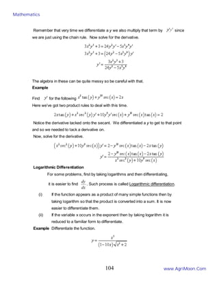
Remember that very time we differentiate a y we also multiply that term by since
we are just using the chain rule. Now solve for the derivative.
Mathematics
www.AgriMoon.Com
32
The algebra in these can be quite messy so be careful with that.
Example:
Find for the following
Here we’ve got two product rules to deal with this time.
Notice the derivative tacked onto the secant. We differentiated a y to get to that point
and so we needed to tack a derivative on.
Now, solve for the derivative.
Logarithmic Differentiation
For some problems, first by taking logarithms and then differentiating,
it is easier to find
dx
dy
. Such process is called Logarithmic differentiation.
(i) If the function appears as a product of many simple functions then by
taking logarithm so that the product is converted into a sum. It is now
easier to differentiate them.
(ii) If the variable x occurs in the exponent then by taking logarithm it is
reduced to a familiar form to differentiate.
Example: Differentiate the function.
Mathematics
www.AgriMoon.Com
33
Solution
Differentiating this function could be done with a product rule and a quotient rule. We
can simplify things somewhat by taking logarithms of both sides.
Example
Differentiate
Solution
First take the logarithm of both sides as we did in the first example and use the logarithm
properties to simplify things a little.
Differentiate both sides using implicit differentiation.
As with the first example multiply by y and substitute back in for y.
PARAMETRIC FUNCTIONS
Sometimes variables x and y are expressed in terms of a third variable called
parameter. We find
dx
dy
without eliminating the third variable.
Let x = f(t) and y = g(t) then
Mathematics
www.AgriMoon.Com
34
dx
dy
=
dx
dt
dt
dy
×
=
dt
dx
dt
dy 1
× =
dt
dx
dt
dy
Problem
1. Find for the parametric function x =a cosθ , y = b sinθ
Solution
θ
θ
sin
a
d
dx
−
= θ
θ
cos
b
d
dy
=
dx
dy
=
θ
θ
d
dx
d
dy
=
θ
θ
sin
cos
a
b
−
= θ
cot
a
b
−
Inference of the differentiation
Let y = f(x) be a given function then the first order derivative is
dx
dy
.
The geometrical meaning of the first order derivative is that it represents the slope of the
curve y = f(x) at x.
The physical meaning of the first order derivative is that it represents the rate of change
of y with respect to x.
PROBLEMS ON HIGHER ORDER DIFFERENTIATION
The rate of change of y with respect x is denoted by
dx
dy
and called as the first
order derivative of function y with respect to x.
Mathematics
www.AgriMoon.Com
35
The first order derivative of y with respect to x is again a function of x, which
again be differentiated with respect to x and it is called second order derivative of y = f(x)
and is denoted by 2
2
dx
y
d
which is equal to 





dx
dy
dx
d
In the similar way higher order differentiation can be defined. Ie. The nth order derivative
of y=f(x) can be obtained by differentiating n-1th
derivative of y=f(x)








=
−
−
1
1
n
n
n
n
dx
y
d
dx
d
dx
y
d
where n= 2,3,4,5….
Problem
Find the first, second and third derivative of
1. y = b
ax
e +
2. y = log(a-bx)
3. y = sin (ax+b)
Partial Differentiation
So far we considered the function of a single variable y = f(x) where x is the only
independent variable. When the number of independent variable exceeds one then we
call it as the function of several variables.
Example
z = f(x,y) is the function of two variables x and y , where x and y are independent
variables.
U=f(x,y,z) is the function of three variables x,y and z , where x, y and z are independent
variables.
In all these functions there will be only one dependent variable.
Consider a function z = f(x,y). The partial derivative of z with respect to x denoted by
x
z
∂
∂
and is obtained by differentiating z with respect to x keeping y as a constant.
Similarly the partial derivative of z with respect to y denoted by
y
z
∂
∂
and is obtained by
differentiating z with respect to y keeping x as a constant.
Problem
1. Differentiate U = log (ax+by+cz) partially with respect to x, y & z
We can also find higher order partial derivatives for the function z = f(x,y) as
follows
Mathematics
www.AgriMoon.Com
36
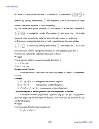
(i) The second order partial derivative of z with respect to x denoted as
2
2
x
z
x
z
x ∂
∂
=






∂
∂
∂
∂
is
obtained by partially differentiating
x
z
∂
∂
with respect to x. this is also known as direct
second order partial derivative of z with respect to x.
(ii)The second order partial derivative of z with respect to y denoted as
2
2
y
z
y
z
y ∂
∂
=








∂
∂
∂
∂
is
obtained by partially differentiating
y
z
∂
∂
with respect to y this is also known as direct
second order partial derivative of z with respect to y
(iii) The second order partial derivative of z with respect to x and then y denoted as
x
y
z
x
z
y ∂
∂
∂
=






∂
∂
∂
∂ 2
is obtained by partially differentiating
x
z
∂
∂
with respect to y. this is also
known as mixed second order partial derivative of z with respect to x and then y
iv) The second order partial derivative of z with respect to y and then x denoted as
y
x
z
y
z
x ∂
∂
∂
=








∂
∂
∂
∂ 2
is obtained by partially differentiating
y
z
∂
∂
with respect to x. this is also
known as mixed second order partial derivative of z with respect to y and then x. In
similar way higher order partial derivatives can be found.
Problem
Find all possible first and second order partial derivatives of
1) z = sin(ax +by)
2) u = xy + yz + zx
Homogeneous Function
A function in which each term has the same degree is called a homogeneous
function.
Example
1) x2
–2xy + y2
= 0 → homogeneous function of degree 2.
2) 3x +4y = 0 → homogeneous function of degree 1.
3) x3
+3x2
y + xy2
– y3
= 0 → homogeneous function of degree 3.
To find the degree of a homogeneous function we proceed as follows:
Consider the function f(x,y) replace x by tx and y by ty if f (tx, ty) = tn
f(x, y) then n
gives the degree of the homogeneous function. This result can be extended to any
number of variables.
Mathematics
www.AgriMoon.Com
37
Problem
Find the degree of the homogeneous function
1.
f(x, y) = x2
–2xy + y2
2. f(x,y) =
y
x
y
x
+
−
Euler’s theorem on homogeneous function
If U= f(x,y,z) is a homogeneous function of degree n in the variables x, y & z then
u
n
z
u
z
y
u
y
x
u
x .
. =
∂
∂
+
∂
∂
+
∂
∂
Problem
Verify Euler’s theorem for the following function
1. u(x,y) = x2
–2xy + y2
2. u(x,y) = x3
+ y3
+ z3
–3xyz
INCREASING AND DECREASING FUNCTION
Increasing function
A function y= f(x) is said to be an increasing function if f(x1) < f(x2) for all x1 < x2.
The condition for the function to be increasing is that its first order derivative is always
greater than zero .
i.e
dx
dy
>0
Decreasing function
A function y= f(x) is said to be a decreasing function if f(x1) > f(x2) for all x1 < x2.
The condition for the function to be decreasing is that its first order derivative is always
less than zero .
i.e
dx
dy
< 0
Problems
1. Show that the function y = x3
+ x is increasing for all x.
2. Find for what values of x is the function y = 8 + 2x – x2
is increasing or decreasing ?
Mathematics
www.AgriMoon.Com
38
Maxima and Minima Function of a single variable
A function y = f(x) is said to have maximum at x = a if f(a) > f(x) in the
neighborhood of the point x = a and f(a) is the maximum value of f(x) . The point x = a is
also known as local maximum point.
A function y = f(x) is said to have minimum at x = a if f(a) < f(x) in the neighborhood
of the point x = a and f(a) is the minimum value of f(x) . The point x = a is also known as
local minimum point.
The points at which the function attains maximum or minimum are called the
turning points or stationary points
A function y=f(x) can have more than one maximum or minimum point .
Maximum of all the maximum points is called Global maximum and minimum of all
the minimum points is called Global minimum.
A point at which neither maximum nor minimum is called Saddle point.
[Consider a function y = f(x). If the function increases upto a particular point x = a and
then decreases it is said to have a maximum at x = a. If the function decreases upto a
point x = b and then increases it is said to have a minimum at a point x=b.]
The necessary and the sufficient condition for the function y=f(x) to have a
maximum or minimum can be tabulated as follows
Maximum Minimum
First order or necessary
condition dx
dy
= 0
dx
dy
=0
Second order or sufficient
condition 2
2
dx
y
d
< 0 2
2
dx
y
d
> 0
Working Procedure
1. Find
dx
dy
and 2
2
dx
y
d
2. Equate
dx
dy
=0 and solve for x. this will give the turning points of the function.
3. Consider a turning point x = a then substitute this value of x in 2
2
dx
y
d
and find the
nature of the second derivative. If
a
x
at
dx
y
d
=








2
2
< 0, then the function has a maximum
Mathematics
www.AgriMoon.Com
39
value at the point x = a. If
a
x
at
dx
y
d
=








2
2
> 0, then the function has a minimum value at
the point x = a.
4. Then substitute x = a in the function y = f(x) that will give the maximum or minimum
value of the function at x = a.
Problem
Find the maximum and minimum values of the following function
1. y = x3
– 3x +1
Mathematics
www.AgriMoon.Com
40
Differential Equations
Differential equation is an equation in which differential coefficients occur.
A differential equation is of two types
(1) Ordinary differential equation
(2) Partial differential equation
An ordinary differential equation is one which contains a single independent variable.
Example:
x
sin
2
dx
dy
= x
e
y
4
dx
dy
=
+
A partial differential equation is one containing more than one independent variable.
Examples
1. z
y
z
y
x
z
x =
∂
∂
+
∂
∂
2. 0
y
z
x
z
2
2
2
2
=
∂
∂
+
∂
∂
Here we deal with only ordinary differential equations.
Definitions
Order
The order of a differential equation is the order of the highest order derivative
appearing in it.
x
e
y
4
dx
dy
=
+ Order 1
0
y
3
dx
dy
4
dx
y
d
2
2
2
=
−






+ Order -2
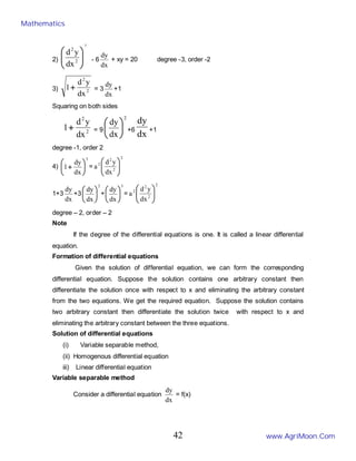
Degree
The degree of a differential equation is defined as the degree of highest ordered
derivative occurring in it after removing the radical sign.
Example
Give the degree and order of the following differential equation.
1) 5 (x+y)
dx
dy
+ 3xy = x2
degree -1, order -1
Mathematics
www.AgriMoon.Com
41
2)
3
2
2
dx
y
d








- 6
dx
dy
+ xy = 20 degree -3, order -2
3) 2
2
dx
y
d
1+ = 3
dx
dy
+1
Squaring on both sides
2
2
dx
y
d
1+ = 9
2
dx
dy






+6
dx
dy
+1
degree -1, order 2
4)
3
dx
dy
1 





+ =
2
2
2
2
dx
y
d
a 







1+3
dx
dy
+3
2
dx
dy






+
3
dx
dy






=
2
2
2
2
dx
y
d
a 







degree – 2, order – 2
Note
If the degree of the differential equations is one. It is called a linear differential
equation.
Formation of differential equations
Given the solution of differential equation, we can form the corresponding
differential equation. Suppose the solution contains one arbitrary constant then
differentiate the solution once with respect to x and eliminating the arbitrary constant
from the two equations. We get the required equation. Suppose the solution contains
two arbitrary constant then differentiate the solution twice with respect to x and
eliminating the arbitrary constant between the three equations.
Solution of differential equations
(i) Variable separable method,
(ii) Homogenous differential equation
iii) Linear differential equation
Variable separable method
Consider a differential equation
dx
dy
= f(x)
Mathematics
www.AgriMoon.Com
42
Here we separate the variables in such a way that we take the terms containing variable
x on one side and the terms containing variable y on the other side. Integrating we get
the solution.
Note
The following formulae are useful in solving the differential equations
(i) d(xy) = xdy +ydx
(ii) 2
y
xdy
ydx
y
x
d
−
=








(iii) 2
x
ydx
xdy
x
y
d
−
=






Homogenous differential equation
Consider a differential equation of the form
( )
( )
y
,
x
f
y
,
x
f
dx
dy
2
1
= (i)
where f1 and f2 are homogeneous functions of same degree in x and y.
Here put y = vx
∴
dx
dv
x
v
dx
dy
+
= (ii)
Substitute equation(ii) in equation (i) it reduces to a differential equation in the variables
v and x. Separating the variables and integrating we can find the solution.
Linear differential equation
A linear differential equation of the first order is of the form Q
py
dx
dy
=
+ , Where
p and Q are functions of x only.
To solve this equation first we find the integrating factor given by
Integrating factor = I.F = ∫pdx
e
Then the solution is given by
∫ +
∫
=
∫ c
dx
e
Q
ye
pdx
pdx
where c is an arbitrary constant.
Mathematics
www.AgriMoon.Com
43
r
C(h,k)
P(x,y)
Circles
A circle is defined as the locus of the point, which moves in such a way, that its
distance from a fixed point is always constant. The fixed point is called centre of the
circle and the constant distance is called the radius of the circle.
The equation of the circle when the centre and radius are given
Let C (h,k) be the centre and r be the radius of the circle. Let P(x,y) be any point
on the circle.
CP = r ⇒CP2
= r2
⇒(x-h)2
+ (y-k)2
= r2
is the required equation of the circle.
Y
X
O
Note :
If the center of the circle is at the origin i.e., C(h,k)=(0,0) then the equation of the
circle is x2
+ y2
= r2
The general equation of the circle is x2
+ y2
+2gx + 2fy + c = 0
Consider the equation x2
+ y2
+2gx + 2fy + c = 0. This can be written as
x2
+ y2
+ 2gx +2fy + g2
+ f2
= g2
+f2
– c
(i.e) x2
+ 2gx + g2
+ y2
+2fy + f2
= g2
+f2
– c
(x + g)2
+ (y + f )2
=
2
2
2






−
+ c
f
g
( )
[ ]2
g
x −
− + ( )
[ ]2
f
y −
− =
2
2
2






−
+ c
f
g
This is of the form (x-h)2
+ (y-k)2
= r2
∴The considered equation represents a circle with centre (-g,-f) and radius c
f
g −
+ 2
2
∴ The general equation of the circle is x2
+ y2
+2gx + 2fy + c = 0
where
c = The Center of the circle whose coordinates are (-g,-f)
r = The radius of the circle = c
f
g −
+ 2
2
Mathematics
www.AgriMoon.Com
44
Note
The general second degree equation
ax2
+ by2
+2hxy + 2gx + 2fy +c = 0
Represents a circle if
(i) a = b i.e., coefficient of x2
= coefficient of y2
(ii) h = 0 i.e., no xy term
Mathematics
www.AgriMoon.Com
45
CHAIN RULE DIFFERENTIATION
If y is a function of u ie y = f(u) and u is a function of x ie u = g(x) then y is related
to x through the intermediate function u ie y =f(g(x) )
∴y is differentiable with respect to x
Furthermore, let y=f(g(x)) and u=g(x), then
dx
dy
=
du
dy
dx
du
There are a number of related results that also go under the name of "chain
rules." For example, if y=f(u) u=g(v), and v=h(x),
then
dx
dy
=
dx
dv
dv
du
du
dy
.
.
Problem
Differentiate the following with respect to x
1. y = (3x2
+4)3
2. y =
2
−
x
e
Marginal Analysis
Let us assume that the total cost C is represented as a function total output q.
(i.e) C= f(q).
Then marginal cost is denoted by MC=
dq
dc
The average cost =
Q
TC
Similarly if U = u(x) is the utility function of the commodity x then
the marginal utility MU =
dx
dU
The total revenue function TR is the product of quantity demanded Q and the price P per
unit of that commodity then TR = Q.P = f(Q)
Then the marginal revenue denoted by MR is given by
dQ
dR
The average revenue =
Q
TR
Problem
1. If the total cost function is C = Q3
- 3Q2
+ 15Q. Find Marginal cost and average cost.
Mathematics
www.AgriMoon.Com
46
Solution
MC =
dq
dc
AC =
Q
TC
2. The demand function for a commodity is P= (a - bQ). Find marginal revenue.
(the demand function is generally known as Average revenue function). Total revenue
TR = P.Q = Q. (a - bQ) and marginal revenue MR=
( )
dq
bQ
aQ
d 2
−
Growth rate and relative growth rate
The growth of the plant is usually measured in terms of dry mater production and
as denoted by W. Growth is a function of time t and is denoted by W=g(t) it is called a
growth function. Here t is the independent variable and w is the dependent variable.
The derivative
dt
dw
is the growth rate (or) the absolute growth rate gr=
dt
dw
. GR =
dt
dw
The relative growth rate i.e defined as the absolute growth rate divided by the total
dry matter production and is denoted by RGR.
i.e RGR =
w
1
.
dt
dw
=
production
matter
dry
total
rate
growth
absolute
Problem
1. If G = at2
+b sin t +5 is the growth function function the growth rate and relative
growth rate.
GR =
dt
dG
RGR =
G
1
.
dt
dG
Implicit Functions
If the variables x and y are related with each other such that f (x, y) = 0 then it is
called Implicit function. A function is said to be explicit when one variable can be
expressed completely in terms of the other variable.
For example, y = x3
+ 2x2
+ 3x + 1 is an Explicit function
xy2
+ 2y +x = 0 is an implicit function
Mathematics
www.AgriMoon.Com
47
Problem
For example, the implicit equation xy=1 can be solved by differentiating implicitly
gives
dx
xy
d )
(
=
dx
d )
1
(
Implicit differentiation is especially useful when y’(x)is needed, but it is difficult or
inconvenient to solve for y in terms of x.
Example: Differentiate the following function with respect to x
Solution
So, just differentiate as normal and tack on an appropriate derivative at each step. Note
as well that the first term will be a product rule.
Example: Find for the following function.
Solution
In this example we really are going to need to do implicit differentiation of x and write y
as y(x).
Notice that when we differentiated the y term we used the chain rule.
Example: Find for the following.
Solutio: First differentiate both sides with respect to x and notice that the first time on
left side will be a product rule.
Remember that very time we differentiate a y we also multiply that term by since
we are just using the chain rule. Now solve for the derivative.
Mathematics
www.AgriMoon.Com
48
The algebra in these can be quite messy so be careful with that.
Example: Find for the following
Here we’ve got two product rules to deal with this time.
Notice the derivative tacked onto the secant. We differentiated a y to get to that point
and so we needed to tack a derivative on.
Now, solve for the derivative.
Logarithmic Differentiation
For some problems, first by taking logarithms and then differentiating,
it is easier to find
dx
dy
. Such process is called Logarithmic differentiation.
(i) If the function appears as a product of many simple functions then by
taking logarithm so that the product is converted into a sum. It is now
easier to differentiate them.
(ii) If the variable x occurs in the exponent then by taking logarithm it is
reduced to a familiar form to differentiate.
Example
Differentiate the function.
Solution
Differentiating this function could be done with a product rule and a quotient
rule. We can simplify things somewhat by taking logarithms of both sides.
Mathematics
www.AgriMoon.Com
49
Example
Differentiate
Solution
First take the logarithm of both sides as we did in the first example and use the logarithm
properties to simplify things a little.
Differentiate both sides using implicit differentiation.
As with the first example multiply by y and substitute back in for y.
PARAMETRIC FUNCTIONS
Sometimes variables x and y are expressed in terms of a third variable called
parameter. We find
dx
dy
without eliminating the third variable.
Let x = f(t) and y = g(t) then
dx
dy
=
dx
dt
dt
dy
×
Mathematics
www.AgriMoon.Com
50
=
dt
dx
dt
dy 1
× =
dt
dx
dt
dy
Problem
1. Find for the parametric function x =a cosθ , y = b sinθ
Solution
θ
θ
sin
a
d
dx
−
= θ
θ
cos
b
d
dy
=
dx
dy
=
θ
θ
d
dx
d
dy
=
θ
θ
sin
cos
a
b
−
= θ
cot
a
b
−
Inference of the differentiation
Let y = f(x) be a given function then the first order derivative is
dx
dy
.
The geometrical meaning of the first order derivative is that it represents the slope of the
curve y = f(x) at x.
The physical meaning of the first order derivative is that it represents the rate of change
of y with respect to x.
PROBLEMS ON HIGHER ORDER DIFFERENTIATION
The rate of change of y with respect x is denoted by
dx
dy
and called as the first
order derivative of function y with respect to x.
The first order derivative of y with respect to x is again a function of x, which
again be differentiated with respect to x and it is called second order derivative of y = f(x)
and is denoted by 2
2
dx
y
d
which is equal to 





dx
dy
dx
d
In the similar way higher order differentiation can be defined. Ie. The nth order derivative
of y=f(x) can be obtained by differentiating n-1th
derivative of y=f(x)
Mathematics
www.AgriMoon.Com
51








=
−
−
1
1
n
n
n
n
dx
y
d
dx
d
dx
y
d
where n= 2,3,4,5….
Problem
Find the first , second and third derivative of
1. y = b
ax
e +
2. y = log(a-bx)
3. y = sin (ax+b)
Partial Differentiation
So far we considered the function of a single variable y = f(x) where x is the only
independent variable. When the number of independent variable exceeds one then we
call it as the function of several variables.
Example
z = f(x,y) is the function of two variables x and y , where x and y are independent
variables.
U=f(x,y,z) is the function of three variables x,y and z , where x, y and z are independent
variables.
In all these functions there will be only one dependent variable.
Consider a function z = f(x,y). The partial derivative of z with respect to x denoted by
x
z
∂
∂
and is obtained by differentiating z with respect to x keeping y as a constant.
Similarly the partial derivative of z with respect to y denoted by
y
z
∂
∂
and is obtained by
differentiating z with respect to y keeping x as a constant.
Problem
1. Differentiate U = log (ax+by+cz) partially with respect to x, y & z
We can also find higher order partial derivatives for the function z = f(x,y) as follows
(i) The second order partial derivative of z with respect to x denoted as
2
2
x
z
x
z
x ∂
∂
=






∂
∂
∂
∂
is
obtained by partially differentiating
x
z
∂
∂
with respect to x. this is also known as direct
second order partial derivative of z with respect to x.
Mathematics
www.AgriMoon.Com
52
(ii)The second order partial derivative of z with respect to y denoted as
2
2
y
z
y
z
y ∂
∂
=








∂
∂
∂
∂
is
obtained by partially differentiating
y
z
∂
∂
with respect to y this is also known as direct
second order partial derivative of z with respect to y
(iii) The second order partial derivative of z with respect to x and then y denoted as
x
y
z
x
z
y ∂
∂
∂
=






∂
∂
∂
∂ 2
is obtained by partially differentiating
x
z
∂
∂
with respect to y. this is also
known as mixed second order partial derivative of z with respect to x and then y
iv) The second order partial derivative of z with respect to y and then x denoted as
y
x
z
y
z
x ∂
∂
∂
=








∂
∂
∂
∂ 2
is obtained by partially differentiating
y
z
∂
∂
with respect to x. this is also
known as mixed second order partial derivative of z with respect to y and then x. In
similar way higher order partial derivatives can be found.
Problem
Find all possible first and second order partial derivatives of
1) z = sin(ax +by)
2) u = xy + yz + zx
Homogeneous Function
A function in which each term has the same degree is called a homogeneous
function.
Example
1) x2
–2xy + y2
= 0 → homogeneous function of degree 2.
2) 3x +4y = 0 → homogeneous function of degree 1.
3) x3
+3x2
y + xy2
– y3
= 0 → homogeneous function of degree 3.
To find the degree of a homogeneous function we proceed as follows.
Consider the function f(x,y) replace x by tx and y by ty if f (tx, ty) = tn
f(x, y) then n
gives the degree of the homogeneous function. This result can be extended to any
number of variables.
Problem
Find the degree of the homogeneous function
1.
f(x, y) = x2
–2xy + y2
Mathematics
www.AgriMoon.Com
53
2. f(x,y) =
y
x
y
x
+
−
Euler’s theorem on homogeneous function
If U= f(x,y,z) is a homogeneous function of degree n in the variables x, y & z then
u
n
z
u
z
y
u
y
x
u
x .
. =
∂
∂
+
∂
∂
+
∂
∂
Problem
Verify Euler’s theorem for the following function
1. u(x,y) = x2
–2xy + y2
2. u(x,y) = x3
+ y3
+ z3
–3xyz
INCREASING AND DECREASING FUNCTION
Increasing function
A function y= f(x) is said to be an increasing function if f(x1) < f(x2) for all x1 < x2.
The condition for the function to be increasing is that its first order derivative is always
greater than zero .
i.e
dx
dy
>0
Decreasing function
A function y= f(x) is said to be a decreasing function if f(x1) > f(x2) for all x1 < x2.
The condition for the function to be decreasing is that its first order derivative is always
less than zero .
i.e
dx
dy
< 0
Problems
1. Show that the function y = x3
+ x is increasing for all x.
2. Find for what values of x is the function y = 8 + 2x – x2
is increasing or decreasing ?
Maxima and Minima Function of a single variable
A function y = f(x) is said to have maximum at x = a if f(a) > f(x) in the
neighborhood of the point x = a and f(a) is the maximum value of f(x) . The point x = a is
also known as local maximum point.
A function y = f(x) is said to have minimum at x = a if f(a) < f(x) in the neighborhood
of the point x = a and f(a) is the minimum value of f(x) . The point x = a is also known as
local minimum point.
Mathematics
www.AgriMoon.Com
54
The points at which the function attains maximum or minimum are called the
turning points or stationary points
A function y=f(x) can have more than one maximum or minimum point .
Maximum of all the maximum points is called Global maximum and minimum of all
the minimum points is called Global minimum.
A point at which neither maximum nor minimum is called Saddle point.
[Consider a function y = f(x). If the function increases upto a particular point x = a and
then decreases it is said to have a maximum at x = a. If the function decreases upto a
point x = b and then increases it is said to have a minimum at a point x=b.]
The necessary and the sufficient condition for the function y=f(x) to have a
maximum or minimum can be tabulated as follows
Maximum Minimum
First order or necessary
condition dx
dy
= 0
dx
dy
=0
Second order or sufficient
condition 2
2
dx
y
d
< 0 2
2
dx
y
d
> 0
Mathematics
www.AgriMoon.Com
55
Working Procedure
1. Find
dx
dy
and 2
2
dx
y
d
2. Equate
dx
dy
=0 and solve for x. this will give the turning points of the function.
3. Consider a turning point x = a then substitute this value of x in 2
2
dx
y
d
and find the
nature of the second derivative. If
a
x
at
dx
y
d
=








2
2
< 0, then the function has a maximum
value at the point x = a. If
a
x
at
dx
y
d
=








2
2
> 0, then the function has a minimum value at
the point x = a.
4. Then substitute x = a in the function y = f(x) that will give the maximum or minimum
value of the function at x = a.
Problem
Find the maximum and minimum values of the following function
1. y = x3
– 3x +1
Mathematics
www.AgriMoon.Com
56
INTEGRATION
Integration is a process, which is a inverse of differentiation. As the symbol
dx
d
represents differentiation with respect to x, the symbol ∫dx stands for integration with
respect to x.
Definition
If ( )
[ ] ( )
x
F
x
f
dx
d
= then f(x) is called the integral of F(x) denoted by
∫ +
= c
x
f
dx
x
F )
(
)
( . This can be read it as integral of F(x) with respect to x is f(x) + c
where c is an arbitrary constant. The integral ∫ dx
x
F )
( is known as Indefinite integral
and the function F(x) as integrand.
Formula on integration
1).
1
1
+
=
+
∫ n
x
dx
x
n
n
+c ( n ≠-1)
2). ∫ = x
dx
x
log
1
+c
3). ∫dx= x+c
4). ∫ =
a
a
dx
a
x
x
log
+c
5). ∫
x
e dx = ex
+c
6). ∫ ∫ +
=
+ dx
x
u
dx
x
v
x
u )
(
))
(
)
(
( ∫ dx
x
v )
(
7). ∫ ∫ ∫
±
=
± dx
x
v
c
dx
x
u
c
dx
x
v
c
x
u
c )
(
)
(
))
(
)
(
( 2
1
2
1
8). ∫cdx= c x + d
9). ∫ −
= x
dx
x cos
sin +c
10). ∫ = x
dx
x sin
cos +c
Mathematics
www.AgriMoon.Com
57
11). ∫ = x
xdx tan
sec2
+c
12). ∫ −
= x
xdx
ec cot
cos 2
+c
13). c
x
dx
x
x +
=
∫ sec
tan
sec
14). c
x
ec
dx
x
ecx
∫ +
−
= cos
cot
cos
13).
a
x
a
dx
x
a
∫
−
=
+
1
2
2
tan
1
1
+c
14). ∫ −
+
=
− x
a
x
a
a
dx
x
a
log
2
1
1
2
2 +c
15).
a
x
a
x
a
dx
a
x +
−
=
−
∫ log
2
1
1
2
2
+c
16). c
x
dx
x
+
=
−
∫
−1
2
tan
1
1
Definite integral
If f(x) is indefinite integral of F(x) with respect to x then the Integral dx
x
F
b
a
∫ )
( is called
definite integral of F(x) with respect to x from x = a to x = b. Here a is called the Lower
limit and b is called the Upper limit of the integral.
dx
x
F
b
a
∫ )
( = [ ]b
a
x
f )
( = f(Upper limit ) - f(Lower limit)
= f(b) - f(a)
Note
While evaluating a definite integral no constant of integration is to be added. That is a
definite integral has a definite value.
Method of substitution
Method –1
Formulae for the functions involving (ax + b)
Consider the integral
Mathematics
www.AgriMoon.Com
58
I = ( ) dx
b
ax
n
∫ + -------------(1)
Where a and b are constants
Put a x + b = y
Differentiating with respect to x
a dx + 0 = dy
a
dy
dx =
Substituting in (1)
I = dy
a
yn 1
.
∫ +c
= dy
y
a
n
.
1
∫ +c
=
1
1 1
+
+
n
y
a
n
+c
=
( )








+
+ +
1
1 1
n
b
ax
a
n
+ c
Similarly this method can be applied for other formulae also.
Method II
Integrals of the functions of the form
( ) dx
x
x
f n
n 1
−
∫
put n
x =y,
dx
dy
nxn
=
−1
n
dy
dx
xn
=
−1
Substituting we get
I = ( )
n
dy
y
f
∫ and this can be integrated.
Method –III
Integrals of function of the type
Mathematics
www.AgriMoon.Com
59
( )
[ ] ( )dx
x
f
x
f
n 1
∫
when n ≠ -1, put f(x) = y then ( ) dy
dx
x
f =
1
∴ ( )
[ ] ( )dx
x
f
x
f
n 1
∫ = dy
y
n
∫
=
1
1
+
+
n
yn
=
( )
[ ]
1
1
+
+
n
x
f n
when n= -1, the integral reduces to
( )
( )
dx
x
f
x
f 1
putting y = f(x) then dy = f1
(x) dx
∴ y
y
dy
log
=
∫ =log f(x)
Method IV
Method of Partial Fractions
Integrals of the form ∫ +
+ c
bx
ax
dx
2
Case.1
If denominator can be factorized into linear factors then we write the integrand as
the sum or difference of two linear factors of the form
d
cx
B
b
ax
A
d
cx
b
ax
c
bx
ax +
+
+
=
+
+
=
+
+ )
)(
(
1
(
1
2
Case-2
In the given integral ∫ +
+ c
bx
ax
dx
2
the denominator ax2
+ bx + c can not be
factorized into linear factors, then express ax2
+ bx + c as the sum or difference of two
perfect squares and then apply the formulae
a
x
a
dx
x
a
∫
−
=
+
1
2
2
tan
1
1
∫ −
+
=
− x
a
x
a
a
dx
x
a
log
2
1
1
2
2
Mathematics
www.AgriMoon.Com
60
a
x
a
x
a
dx
a
x +
−
=
−
∫ log
2
1
1
2
2
Integrals of the form∫
+
+ c
bx
ax
dx
2
Write denominator as the sum or difference of two perfect squares
∫
+
+ c
bx
ax
dx
2
= ∫
+ 2
2
a
x
dx
or ∫
− 2
2
a
x
dx
or ∫
− 2
2
x
a
dx
and then apply the formula
∫
+ 2
2
a
x
dx
= log(x+ )
2
2
a
x +
∫
− 2
2
a
x
dx
= log(x+ )
2
2
a
x −
∫
− 2
2
x
a
dx
= 





−
a
x
1
sin
Integration by parts
If the given integral is of the form ∫udv then this can not be solved by any of
techniques studied so far. To solve this integral we first take the product rule on
differentiation
dx
uv
d )
(
=u
dx
dv
+v
dx
du
Integrating both sides we get
∫ dx
uv
d )
(
dx= ∫ ( u
dx
dv
+v
dx
du
)dx
then we have u v= ∫vdu+ ∫udv
re arranging the terms we get
∫udv = uv- ∫vdu This formula is known as integration by parts formula
Select the functions u and dv appropriately in such a way that integral ∫vdu can be more
easily integrable than the given integral
Mathematics
www.AgriMoon.Com
61
APPLICATION OF INTEGRATION
The area bounded by the function y=f(x), x=axis and the ordinates at x=a x=b is
given by ∫
=
b
a
dx
x
f
A )
(
Mathematics
www.AgriMoon.Com
62
1
INVERSE OF AMATRIX
Definition
Let A be any square matrix. If there exists another square matrix B Such that AB
= BA = I (I is a unit matrix) then B is called the inverse of the matrix A and is denoted by
A-1
.
The cofactor method is used to find the inverse of a matrix. Using matrices, the
solutions of simultaneous equations are found.
Working Rule to find the inverse of the matrix
Step 1: Find the determinant of the matrix.
Step 2: If the value of the determinant is non zero proceed to find the inverse of the
matrix.
Step 3: Find the cofactor of each element and form the cofactor matrix.
Step 4: The transpose of the cofactor matrix is the adjoint matrix.
Step 5: The inverse of the matrix A-1
=
A
A
adj )
(
Example
Find the inverse of the matrix










9
4
1
3
2
1
1
1
1
Solution
Let A =










9
4
1
3
2
1
1
1
1
Step 1
0
2
2
6
6
)
2
4
(
)
3
9
(
1
)
12
18
(
1
9
4
1
3
2
1
1
1
1
≠
=
+
−
=
−
+
−
−
−
=
=
A
Step 2
The value of the determinant is non zero
∴A-1
exists.
Step 3
Let Aij denote the cofactor of aij in A
Mathematics
www.AgriMoon.Com
63
2
( ) 6
12
18
9
4
3
2
1
1
1
1
11 =
−
=
−
=
=
+
of
Cofactor
A
( ) 6
)
3
9
(
9
1
3
1
1
1
3
1
12 −
=
−
−
=
−
=
=
+
of
Cofactor
A
( ) 2
2
4
4
1
2
1
1
1
3
1
13 =
−
=
−
=
=
+
of
Cofactor
A
( ) 5
)
4
9
(
9
4
1
1
1
1
1
2
21 −
=
−
−
=
−
=
=
+
of
Cofactor
A
( ) 8
1
9
9
1
1
1
1
2
2
2
22 =
−
=
−
=
=
+
of
Cofactor
A
( ) 3
)
1
4
(
4
1
1
1
1
3
3
2
23 −
=
−
−
=
−
=
=
+
of
Cofactor
A
( ) 1
2
3
3
2
1
1
1
1
1
3
31 =
−
=
−
=
=
+
of
Cofactor
A
( ) 2
)
1
3
(
3
1
1
1
1
4
2
3
32 −
=
−
−
=
−
=
=
+
of
Cofactor
A
( ) 1
1
2
2
1
1
1
1
9
3
3
33 =
−
=
−
=
=
+
of
Cofactor
A
Step 4
The matrix formed by cofactors of element of determinant A is










−
−
−
−
1
2
1
3
8
5
2
6
6
∴adj A =










−
−
−
−
1
3
2
2
8
6
1
5
6
Step 5










−
−
−
−
=
=
−
1
3
2
2
8
6
1
5
6
2
1
1
A
A
adj
A
=
















−
−
−
−
2
1
2
3
1
1
4
3
2
1
2
5
3
Mathematics
www.AgriMoon.Com
64
3
SOLUTION OF LINEAR EQUATIONS
Let us consider a system of linear equations with three unknowns
3
3
3
3
2
2
2
2
1
1
1
1
d
z
c
y
b
x
a
d
z
c
y
b
x
a
d
z
c
y
b
x
a
=
+
+
=
+
+
=
+
+
The matrix form of the equation is AX=B where
3
3
3
2
2
2
1
1
1
c
b
a
c
b
a
c
b
a
A = is a 3x3 matrix
X =










z
y
x
and B =










3
2
1
d
d
d
Here AX = B
Pre multiplying both sides by A-1
.
(A-1
A)X= A-1
B
We know that A-1
A= A A-1
=I
∴ I X= A-1
B
since IX = X
Hence the solution is X = A-1
B.
Example
Solve the x + y + z = 1, 3x + 5y + 6z = 4, 9x + 26y + 36z =16 by matrix method.
Solution
The given equations are x + y + z = 1,
3x + 5y + 6z = 4,
9x + 26y + 36z =16
Let A=










36
26
9
6
5
3
1
1
1
, X=










z
y
x
, B=










16
4
1
The given system of equations can be put in the form of the matrix equation AX=B
0
3
33
54
24
)
45
78
(
1
)
54
108
(
1
)
156
180
(
1
36
26
9
6
5
3
1
1
1
≠
=
+
−
=
−
+
−
−
−
=
=
A
Mathematics
www.AgriMoon.Com
65
4
The value of the determinant is non zero
∴ A-1
exists.
Let Aij (i, j = 1,2,3) denote the cofactor of aij in A
( ) 24
156
180
36
26
6
5
1
1
1
1
11 =
−
=
−
=
=
+
of
Cofactor
A
( ) 54
)
54
108
(
36
9
6
3
1
1
3
1
12 −
=
−
−
=
−
=
=
+
of
Cofactor
A
( ) 33
45
78
26
9
5
3
1
1
3
1
13 =
−
=
−
=
=
+
of
Cofactor
A
( ) 10
)
26
36
(
36
26
1
1
1
3
1
2
21 −
=
−
−
=
−
=
=
+
of
Cofactor
A
( ) 27
9
36
36
9
1
1
1
5
2
2
22 =
−
=
−
=
=
+
of
Cofactor
A
( ) 17
)
9
26
(
26
9
1
1
1
6
3
2
23 −
=
−
−
=
−
=
=
+
of
Cofactor
A
( ) 1
5
6
6
5
1
1
1
9
1
3
31 =
−
=
−
=
=
+
of
Cofactor
A
( ) 3
)
3
6
(
6
3
1
1
1
26
2
3
32 −
=
−
−
=
−
=
=
+
of
Cofactor
A
( ) 2
3
5
5
3
1
1
1
36
3
3
33 =
−
=
−
=
=
+
of
Cofactor
A
The matrix formed by cofactors of element of determinant A is










−
−
−
−
2
3
1
17
27
10
33
54
24
∴adj A =










−
−
−
−
2
17
33
3
27
54
1
10
24










−
−
−
−
=
=
−
2
17
33
3
27
54
1
10
24
3
1
1
A
A
adj
A
We Know that X=A-1
B
Mathematics
www.AgriMoon.Com
66
5
∴










z
y
x
=










−
−
−
−
2
17
33
3
27
54
1
10
24
3
1










16
4
1










+
−
+
−
+
+
−
+
−
+
=
16
.
2
4
)
17
(
1
.
33
16
)
3
(
4
.
27
1
)
54
(
16
.
1
4
)
10
(
1
.
24
3
1










−
=
3
6
0
3
1
=










−1
2
0
x = 0, y = 2, z = -1.
SOLUTION BY DETERMINANT (CRAMER'S RULE)
Let the equations be
……………………. (1)
Consider the determinant
3
3
3
2
2
2
1
1
1
c
b
a
c
b
a
c
b
a
=
∆
3
3
3
2
2
2
1
1
1
c
b
d
c
b
d
c
b
d
x =
∆
3
3
3
2
2
2
1
1
1
c
d
a
c
d
a
c
d
a
y =
∆
3
3
3
2
2
2
1
1
1
d
b
a
d
b
a
d
b
a
z =
∆
When ∆ ≠ 0, the unique solution is given by
∆
∆
=
∆
∆
=
∆
∆
= z
y
x
z
y
x ,
,
Example
Solve the equations x + 2y + 5z =23, 3x + y + 4z = 26, 6x + y + 7z = 47
by determinant method (Cramer’s Rule).
Solution
The equations are
x + 2y + 5z =23,
3x + y + 4z = 26,
6x + y + 7z = 47
Mathematics
www.AgriMoon.Com
67
6
;
0
6
7
1
6
4
1
3
5
2
1
≠
−
=
=
∆ ;
24
7
1
47
4
1
26
5
2
23
−
=
=
∆x
12
7
47
6
4
26
3
5
23
1
−
=
=
∆y 18
47
1
6
26
1
3
23
2
1
−
=
=
∆z
By Cramer’s rule
3
6
18
2
6
12
4
6
24
=
−
−
=
∆
∆
=
=
−
−
=
∆
∆
=
=
−
−
=
∆
∆
=
z
y
x
z
y
x
⇒ x = 4, y = 2, z = 3.
Mathematics
www.AgriMoon.Com
68
1
MATRICES
An arrangement of numbers in rows and columns. A matrix of type “(m x n)” is
defined as arrangement of (m x n) numbers in ‘m’ rows & ‘n’ columns. Usually these
numbers are enclosed within square brackets [ ] (or) simple brackets ( ) are denoted
by capital letters A, B, C etc.
Example
A = B =
Here A is of type 3 x 4 & B is of type 4 x 3
Types of matrices
1. Row matrix: It is a matrix containing only one row and several columns .It is also
called as row vector.
Example:
[1 3 7 9 6 ]
(1 x 5) matrix called row vector.
2. Column matrix: It is a matrix containing only one column. It is also known as
column vector.
Example:
(3x1)
3. Square matrix: A matrix is called as square matrix, if the number of rows is equal to
number of columns.
Example
The elements a11, a22, a33 etc fall along the diagonal & this is called a leading
diagonal (or) principal diagonal of the matrix.
1 2 3 4
9 10 -1 3
4 2 8 5
1 3 4
2 10 2
9 -1 3
4 8 5
1
4
1
4 2 4
1 9 8
6 5 2
Mathematics
www.AgriMoon.Com
69
2
4. Trace of the matrix
It is defined as the sum of the elements along the leading diagonal.
In this above matrix the trace of the matrix is
4 + 9 + 2 = 15.
5. Diagonal matrix
It is a square matrix in which all the elements other than in the leading diagonals
are zero’s.
Eg:
6.Scalar matrix
It is a diagonal matrix in which all the elements in the leading diagonal are same.
Eg:
7. Unit matrix or identify matrix
It is a diagonal matrix, in which the elements along the leading diagonal are
equal to one. It is denoted by I
I =
8. Zero matrix (or) Non-matrix
It is matrix all of whole elements are equal to zero denoted by “O”
Eg: O = 2 x 3 O = 2 x 2
9. Triangular matrix
There are two types. 1. Lower Triangular Matrix 2. Upper Triangular Matrix.
1 0 0
0 2 0
0 0 3
2 0 0
0 2 0
0 0 2
1 0 0
0 1 0
0 0 1
0 0 0
0 0 0
0 0
0 0
Mathematics
www.AgriMoon.Com
70
3
Lower Triangular matrix
It is a square matrix in which all the elements above the leading diagonal are
zeros.
Eg:
Upper Triangular matrix
Square matrix in which all the elements below the leading diagonal are zeros
Eg:
10. Symmetric matrix
A square matrix A = {aij} said i = 1 to n ; j = 1 to n said
to symmetric, if for all i and j.
Eg:
11. Skew symmetric matrix
A square matrix A = {aij} i = 1 to n , j = 1 to n is called skew symmetric, if
for all i & j. Here aii = 0 for all i
Eg:
Algebra of matrices
1. Equality of matrices
Two matrices A & B are equal, if and only if,
(i) Both A & B are of the same type
(ii) Every element of ‘B’ is the same as the corresponding element of ‘A’.
1
3 1
4 6 2
0 0
0
5 2 6
1 3
4
0
0 0
aij = aij
aij = -aji
0 3 -4
-3 0 5
4 -5 0
1 3 4
3 6 -5
4 -5 2
Mathematics
www.AgriMoon.Com
71
4
Example
1.
A = B =
Here order of matrix A is not same as order matrix B, the two matrices are not
equal.
A ≠ B
2. Find the value of a and b given






=






2
3
5
4
5
4
b
a
Solution:
The given matrices are equal
∴ a = 3, b = 2
2. Addition of matrices
Two matrices A & B can be added if and only if,
(i) Both are of the same type.
(ii) The resulting matrix of A & B is also of same type and is obtained by
adding the all elements of ‘A’ to the corresponding elements of ‘B’.
Example
1. Find 





+






1
2
3
2
6
5
5
4
Solution






+






1
2
3
2
6
5
5
4
= 





+
+
+
+
1
6
2
5
3
5
2
4
= 





7
7
8
6
3. Subtraction of the matrices
This can be done, when both the matrices are of same type.
(A-B) is obtained by subtracting the elements of ‘A’ with corresponding elements of ‘B’.
Example
1. Find 





−






1
2
3
2
6
5
5
4
1 2 3 4
9 10 -1 3
4 2 8 5
1 3 4
2 10 2
9 -1 3
4 8 5
Mathematics
www.AgriMoon.Com
72
5
Solution






−






1
2
3
2
6
5
5
4
= 





−
−
−
−
1
6
2
5
3
5
2
4
= 





5
3
2
2
4. Multiplication of matrix
They are of two types : 1. By a scalar K B.
2. By a matrix A x B.
i) Scalar multiplication
To multiply a matrix ‘A’ by a scalar ‘K’, then multiply every element of a matrix
‘A’ by that scalar.
Example
1. Find 





6
5
5
4
2
Solution:






6
5
5
4
2 = 





12
10
10
8
ii) Matrix Multiplication
Two matrices A & B can be multiplied to form the matrix product AB, if and only if
the number of columns of 1st
matrix A is equal to the number of rows of 2nd
matrix B.
If A is an (m x p) and B is an (p x n) then the matrix product AB can be formed. AB is a
matrix by (m x n).
In this case the matrices A and B are said to be conformable for matrix
multiplication.
Example
1. Find
Solution
= 





−
×
+
×
×
+
×
−
×
+
×
×
+
×
3
5
4
4
2
5
6
4
3
3
4
2
2
3
6
2
= 





−
+
+
−
+
+
15
16
10
24
9
8
6
12
2 3
4 5
6 4
2 -3
2 3
4 5
6 4
2 -3
Mathematics
www.AgriMoon.Com
73
6
2 3
1 0
4 5
= 




 −
1
34
1
18
Note: The matrix product AB is different from the matrix product BA.
1. The matrix AB can be formed but not BA
Eg: A is a (2 x 3) matrix
B is a (3 x 5) matrix
AB alone can be formed and it is a (2 x 5) matrix.
2. Even if AB & BA can be formed, they need not be of same type.
Eg: A is a (2 x 3) matrix
B is a (3 x 2) matrix
AB can be formed and is a (2 x 2) matrix
BA can be formed and is a (3x 3) matrix
3. Even if AB & BA are of the same type, they needn’t be equal. Because, they need not
be identical.
Eg: A is a (3 x 3) matrix
B is a (3 x 3) matrix
AB is a (3 x 3) matrix
BA is a (3x 3) matrix
AB ≠ BA
The multiplication of any matrix with null matrix the resultant matrix is also a null
matrix.
When any matrix (ie.) A is multiplied by unit matrix; the resultant matrix is ‘A’
itself.
Transpose of a matrix
The Transpose of any matrix (‘A’) is obtained by interchanging the rows &
columns of ‘A’ and is denoted by AT
. If A is of type (m x n), then AT
is of type (n x m).
Eg: A =
AT
=
(3 x 2) (2 x 3)
2 1 4
3 0 5
Mathematics
www.AgriMoon.Com
74
7
Properties of transpose of a matrix
1) (AT
)T
= A
2) (AB)T
= BT
AT
is known as the reversal Law of Transpose of product of two
matrices.
DETERMINANTS
Every square matrix A of order n x n with entries real or complex there exists a
number called the determinant of the matrix A denoted by by Aor det (A). The
determinant formed by the elements of A is said to be the determinant of the matrix A..
Consider the 2nd
order determinant.
a1 b1
a2 b2
Eg: 4 3
1 0
Consider the 3rd
order determinant,
a1 b1 c1
a2 b2 c2
a3 b3 c3
This can be expanded along any row or any column. Usually we expand by the
1st
row. On expanding along the 1st
row
b2 c2 a2 c2 a2 b2
b3 c3 a3 c3 a3 b3
Minors
Let A = ( ij
a )be a determinant of order n. The minor of the element ij
a is the
determinant formed by deleting ith
row and jth
column in which the element belongs and
the cofactor of the element is ( ) ij
j
i
ij M
i
A +
−
= where M is the minor of ith
row and jth
column .
Example 1 Calculate the determinant of the following matrices.
A  = = a1 b2 – a2 b1
A  = = 0-3 = -3
A  =
- b1 + c1
A  = a1
Mathematics
www.AgriMoon.Com
75
8
(a)










−1
3
1
4
2
3
3
2
1
Solution
21
21
14
14
)
2
9
(
3
)
4
3
(
2
)
12
2
(
1
3
1
2
3
3
1
1
4
3
2
1
3
4
2
1
1
3
1
4
2
3
3
2
1
=
+
+
−
=
−
+
−
−
−
−
−
=
+
−
−
−
=
−
Singular and Non-Singular Matrices:
Definition
A square matrix ‘A’ is said to be singular if, A  = 0 and it is called non-
singular if A  ≠ 0.
Note
Only square matrices have determinants.
Example: Find the solution for the matrix
3
5
7
0
1
5
3
4
2
A =
0
54
60
6
)
7
25
(
3
)
0
15
(
4
)
0
3
(
2
5
7
1
5
3
3
7
0
5
4
3
5
0
1
2
3
5
7
0
1
5
3
4
2
=
+
−
=
−
+
−
−
−
=
+
−
=
Here A  = 0 .So the given matrix is singular
Properties of determinants
1. The value of a determinant is unaltered by interchanging its rows and columns.
Example
Let










−
=
1
3
1
4
2
3
3
2
1
A then
21
21
14
14
)
2
9
(
3
)
4
3
(
2
)
12
2
(
1
3
1
2
3
3
1
1
4
3
2
1
3
4
2
1
1
3
1
4
2
3
3
2
1
)
(
det
=
+
+
−
=
−
+
−
−
−
−
−
=
+
−
−
−
=
−
=
A
Mathematics
www.AgriMoon.Com
76
9
Let us interchange the rows and columns of A. Thus we get new matrix A1.
Then
21
2
33
14
)
6
8
(
1
)
9
2
(
3
)
12
2
(
1
4
3
2
2
1
1
3
3
2
3
1
4
3
2
1
1
4
3
3
2
2
1
3
1
)
(
det 1
=
+
+
−
=
−
+
−
−
−
−
−
=
+
−
−
−
=
−
=
A
Hence det (A) = det (A1).
2. If any two rows (columns) of a determinant are interchanged the determinant
changes its sign but its numerical value is unaltered.
Example
Let










−
=
1
3
1
4
2
3
3
2
1
A then
21
21
14
14
)
2
9
(
3
)
4
3
(
2
)
12
2
(
1
3
1
2
3
3
1
1
4
3
2
1
3
4
2
1
1
3
1
4
2
3
3
2
1
)
(
det
=
+
+
−
=
−
+
−
−
−
−
−
=
+
−
−
−
=
−
=
A
Let A1 be the matrix obtained from A by interchanging the first and second row. i.e R1
and R2.
Then
21
4
8
33
)
2
3
(
4
)
3
1
(
2
)
9
2
(
3
3
1
2
1
4
1
1
3
1
2
1
3
3
2
3
1
3
1
3
2
1
4
2
3
)
(
det 1
−
=
+
+
−
=
−
+
−
−
−
−
−
=
+
−
−
−
=
−
=
A
Hence det (A) = - det (A1).
3. If two rows (columns) of a determinant are identical then the value of the
terminant is zero.
Example
Let










−
=
1
1
1
4
3
3
3
1
1
A then
Mathematics
www.AgriMoon.Com
77
10
0
0
7
7
)
3
3
(
3
)
4
3
(
1
)
4
3
(
1
1
1
3
3
3
1
1
4
3
1
1
1
4
3
1
1
1
1
4
3
3
3
1
1
)
(
det
=
+
+
−
=
−
+
−
−
−
−
−
=
+
−
−
−
=
−
=
A
Hence 0
)
(
det =
A
4. If every element in a row ( or column) of a determinant is multiplied by a
constant “k” then the value of the determinant is multiplied by k.
Example
Let










−
=
1
3
1
4
2
3
3
2
1
A then
21
21
14
14
)
2
9
(
3
)
4
3
(
2
)
12
2
(
1
3
1
2
3
3
1
1
4
3
2
1
3
4
2
1
1
3
1
4
2
3
3
2
1
)
(
det
=
+
+
−
=
−
+
−
−
−
−
−
=
+
−
−
−
=
−
=
A
Let A1 be the matrix obtained by multiplying the elements of the first row by 2 (ie. here k
=2) then
( ) ( ) ( )
[ ]
[ ] ( )
21
2
21
14
14
2
)
2
9
(
3
)
4
3
(
2
)
12
2
(
1
2
3
1
2
3
3
2
1
1
4
3
2
2
1
3
4
2
1
2
1
3
1
4
2
3
3
2
2
2
1
2
)
(
det 1
=
+
+
−
=
−
+
−
−
−
−
−
=
×
+
−
×
−
−
×
=
−
=
A
Hence det (A) = 2 det (A1).
5. If every element in any row (column) can be expressed as the sum of two
quantities then given determinant can be expressed as the sum of two
determinants of the same order with the elements of the remaining rows
(columns) of both being the same.
Example
Let










−
+
+
+
=
1
3
1
4
2
3
6
3
4
2
2
1
A then
Mathematics
www.AgriMoon.Com
78
11
21
21
14
14
)
2
9
(
3
)
4
3
(
2
)
12
2
(
1
3
1
2
3
3
1
1
4
3
2
1
3
4
2
1
1
3
1
4
2
3
3
2
1
)
1
(
det
)
2
(
det
)
1
(
det
1
3
1
4
2
3
6
4
2
1
3
1
4
2
3
3
2
1
1
3
1
4
2
3
6
3
4
2
2
1
)
(
det
=
+
+
−
=
−
+
−
−
−
−
−
=
+
−
−
−
=
−
=
+
=
−
+
−
=
−
+
+
+
=
M
M
M
A
63
42
21
)
(
det
)
2
(
det
)
1
(
det
)
(
det
42
42
28
28
)
2
9
(
6
)
4
3
(
4
)
12
2
(
2
3
1
2
3
6
1
1
4
3
4
1
3
4
2
2
1
3
1
4
2
3
6
4
2
)
2
(
det
=
+
=
+
=
=
+
+
−
=
−
+
−
−
−
−
−
=
+
−
−
−
=
−
=
A
Hence
M
M
A
M
6. A determinant is unaltered when to each element of any row (column) is added
to those of several other rows (columns) multiplied respectively by constant
factors.
Example
Let










−
=
1
3
1
4
2
3
3
2
1
A then
21
21
14
14
)
2
9
(
3
)
4
3
(
2
)
12
2
(
1
3
1
2
3
3
1
1
4
3
2
1
3
4
2
1
1
3
1
4
2
3
3
2
1
)
(
det
=
+
+
−
=
−
+
−
−
−
−
−
=
+
−
−
−
=
−
=
A
Let A1 be a matrix obtained when the elements C1 of A are added to those of second
column and third column multiplied respectively by constants 2 and 3. Then
Mathematics
www.AgriMoon.Com
79
12
21
21
14
14
)
0
(
3
)
0
(
2
)
2
9
(
3
)
4
3
(
2
)
12
2
(
1
1
3
1
4
2
4
3
2
3
3
1
3
3
4
2
2
3
2
2
2
1
3
1
4
2
3
3
2
1
1
3
)
1
(
3
4
2
)
4
(
3
3
2
)
3
(
3
1
3
)
3
(
2
4
2
)
2
(
2
3
2
)
2
(
2
1
3
1
4
2
3
3
2
1
1
3
)
1
(
3
)
3
(
2
1
4
2
)
4
(
3
)
2
(
2
3
3
2
)
3
(
3
)
2
(
2
1
)
(
det 1
=
+
+
−
=
+
+
−
+
−
−
−
−
−
=
−
−
+
−
+
−
=
−
−
+
−
+
−
=
−
−
+
+
+
+
+
+
=
A
Mathematics
www.AgriMoon.Com
80
PHYSICAL AND ECONOMIC OPTIMUM FOR SINGLE INPUT
Let y = f(x) be a response function. Here x stands for the input that is kgs of
fertilizer applied per hectare and y the corresponding output that is kgs of yield per
hectare.
We know that the maximum is only when 0
dx
dy
= and 0
dx
y
d
2
2
< .
This optimum is called physical optimum. We are not considering the profit with respect
to the investment, we are interested only in maximizing the profit.
Economic optimum
The optimum which takes into consideration the amount invested and returns is
called the economic optimum.
y
x
P
P
dx
dy
=
where Px → stands for the per unit price of input that is price of fertilizer per kgs.
Py → stands for the per unit price of output that is price of yield per kgs.
Problem
The response function of paddy is y = 1400 + 14.34x -0.05 x2
where x represents
kgs of nitrogen/hectare and y represents yield in kgs/hectare. 1 kg of paddy is Rs. 2 and
1 kg of nitrogen is Rs. 5. Find the physical and economic optimum. Also find the
corresponding yield.
Solution
y = 1400 + 14.34x -0.05 x2
x
1
.
0
34
.
14
dx
dy
−
=
1
.
0
dx
y
d
2
2
−
= = negative value
ie. 0
dx
y
d
2
2
<
Therefore the given function has a maximum point.
Physical Optimum
0
dx
dy
=
i.e 14.34-0.1x = 0
-0.1 x = -14.34
Mathematics
www.AgriMoon.Com
81
x = 4
.
143
1
.
0
34
.
14
= kgs/hectare
therefore the physical optimum level of nitrogen is 143.4 kgs/hectare.
Therefore the maximum yield is
Y = 1400 + 14.34(143.4) -0.05(143.4)2
= 2428.178 kgs/ hectare.
Economic optimum
y
x
P
P
dx
dy
=
Given
Price of nitrogen per kg = Px = 5
Price of yield per kg = Py = 2
Therefore =
dx
dy
14.34-0.1x =
2
5
28.68 - 0.2 x = 5
- 0.2 x = 5 - 28.68
x = 4
.
118
2
.
0
68
.
23
= kgs/hectare
therefore the economic optimum level of nitrogen is 118.4 kgs/hectare.
Therefore the maximum yield is
Y = 1400 + 14.34(118.4) -0.05(118.4)2
= 2396.928 kgs/ hectare.
Maxima and Minima of several variables with constraints and without constraints
Consider the function of several variables
y = f (x1, x2……….xn)
where x1, x2 …………..xn are n independent variables and y is the dependent variable.
Working Rule
Step 1: Find all the first order partial derivatives of y with respect to x1, x2, x3 ……xn..
(ie) 1
1
f
x
y
=
∂
∂
2
2
f
x
y
=
∂
∂
Mathematics
www.AgriMoon.Com
82
3
3
f
x
y
=
∂
∂
.
.
.
.
fn
x
y
n
=
∂
∂
Step 2
Find all the second order partial derivatives of y with respect to x1, x2, x3 ….xn
and they are given as follows.
11
2
1
2
f
x
y
=
∂
∂
21
1
2
2
f
x
x
y
=
∂
∂
∂
22
2
2
2
f
x
y
=
∂
∂
12
2
1
2
f
x
x
y
=
∂
∂
∂
33
2
3
2
f
x
y
=
∂
∂
31
1
3
2
f
x
x
y
=
∂
∂
∂
13
3
1
2
f
x
x
y
=
∂
∂
∂
and so on
Step: 3
Construct an Hessian matrix which is formed by taking all the second order
partial derivatives is given by
Mathematics
www.AgriMoon.Com
83


























=
nn
n
n
n
n
n
f
f
f
f
f
f
f
f
f
f
f
f
H
....
..........
.
.
.
.
.
....
..........
....
..........
3
2
1
2
23
22
21
1
13
12
11
H is a symmetric matrix.
Step: 4
Consider the following minors of order 1, 2, 3 ……….
11
11
1 f
f
H =
=
22
21
12
11
2
f
f
f
f
H =
nn
n
n
n
n
n
n
f
f
f
f
f
f
f
f
f
f
f
f
H
f
f
f
f
f
f
f
f
f
H
....
..........
.
.
.
.
.
.
.
.
.
.
.
.
.
.
.
.
....
..........
....
..........
.
.
.
.
.
3
2
1
2
23
22
21
1
13
12
11
33
32
31
23
22
21
13
12
11
3
=
=
Mathematics
www.AgriMoon.Com
84
Steps: 5
The necessary condition for finding the maximum or minimum
Equate the first order derivative to zero (i.e) f1 = f2 = ……..fn = 0 and find the
value of x1, x2, ……..xn.
Steps: 6
Substitute the values x1, x2 ……..xn in the Hessian matrix. Find the values of
n
H
H
H
H ..
..........
,
, 3
2
1
If
.
..........
0
0
0
0
4
3
2
1
on
so
and
H
H
H
H
>
<
>
<
Then the function is maximum at x1, x2 ……..xn.
If .........
0
,
0
,
0 3
2
1 >
>
> H
H
H then the function is minimum
at x1, x2……. xn.
Steps: 7
Conditions Maximum Minimum
First f1 = f2 = f3 = fn = 0 f1 = 0, f2 = 0 ……. fn = 0
Second
0
0
0
3
2
1
<
>
<
H
H
H
……….
.
.
.
0
0
0
3
2
1
>
>
>
H
H
H
Note :
If the second order conditions are not satisfied then they are called saddle point.
Problem
Find the maxima (or) minima if any of the following function.
)
1
__(
__________
x
8
x
4
x
x
3
4
y 2
1
2
2
3
1 +
−
+
=
Solution
Step 1: The first order partial derivatives are
Mathematics
www.AgriMoon.Com
85
4
4
2
1
1
1 −
=
∂
∂
= x
x
y
f
8
2 2
2
2 +
=
∂
∂
= x
x
y
f
Step 2: The second order partial derivatives are
1
2
1
2
11 8x
x
y
f =
∂
∂
=
0
1
2
2
21 =
∂
∂
∂
=
x
x
y
f
2
2
2
2
22 =
∂
∂
=
x
y
f
0
2
1
2
12 =
∂
∂
∂
=
x
x
y
f
Step 3: The Hessian matrix is 





=
22
21
12
11
f
f
f
f
H






=
2
0
0
x
8
H
1
4. Equate f1, f2 = 0
f1 ⇒ 4x1
2 -
4 = 0
x1
2
= 1
x1 = ± 1
x1 = 1, x1 = -1
f2 ⇒ 2 x 2 + 8=0
2 x2 = - 8
x2 = - 4
The stationary points are (1,- 4) & (-1, - 4)
At the point (1, - 4) the Hessian matrix will be
H = 





2
0
0
8
Mathematics
www.AgriMoon.Com
86
| H1 | = | 8| > 0
| H2 | = 





2
0
0
8
= 16 > 0
Since the determinant H1 and H2 are positive the function is minimum at (1, - 4).
The minimum value at x1 = 1 & x2 = - 4 is obtained by substituting the values
in (1)
y =
3
4
(1) 3
+ (- 4)2
– 4 (1) + 8 (- 4)
y =
3
4
+ 16 – 4 - 32
y =
3
4
- 20
y =
3
60
4 −
=
3
56
−
The minimum value is
3
56
−
At the point (-1, - 4)
H =
2
0
0
8
−
| H1 | = | - 8 | = - 8 < 0
| H 2| = - 16 < 0
Both the conditions are not satisfied. Hence the point (-1, - 4) gives a saddle point.
Economic Optimum
For finding the Economic Optimum we equate the first order derivative
f1 . f 2 . . . . fn to the inverse ratio of the unit prices.
(ie) f1 =
y
x
1 p
p
x
y 1
=
∂
∂
f2 =
y
x
2 p
p
x
y 2
=
∂
∂
…………..
fn =
y
x
n p
p
x
y n
=
∂
∂
Mathematics
www.AgriMoon.Com
87
where Px1 , Px2,… Pxn and Py are the unit prices of x1, x2 ….. xn and y. These are
the first order condition.
The economic optimum & the physical optimum differ only in the first order
conditions. The other procedures are the same.
Maxima & Minima of several variables under certain condition with constraints.
Consider the response function
y = f (x1, x2 …. xn ) subject to the constraint φ (x1, x2….. xn ) =0
The objective function is Z= f(x1, x2, …xn) + λ[φ(x1, x2, …xn)]
where λ is called the Lagrange’s multiplies.
The partial derivatives are
fi
x
z
i
=
∂
∂
for i = 1, 2 ….. n.
ij
1
i
2
f
x
x
z
=
∂
∂
∂ i, j = 1., 2 …. n.
i
xi
φ
φ
=
∂
∂ i = 1, 2 ….. n.
Now form the Bordered Hessian Matrix as follows.
Bordered Hessian




















=
nn
n
n
n
n
f
f
f
f
f
f
f
f
f
H
..
..........
.
.
.
..
..........
..
..........
....
..........
0
2
1
2
2
22
21
2
1
12
11
1
2
1
φ
φ
φ
φ
φ
φ
[Since this extra row & column is on the border of the matrix










nn
n
n
n
n
f
f
f
f
f
f
f
f
f
........
.........
.........
2
1
2
22
21
1
12
11
.So
we call it as Bordered Hessian matrix and it is denoted by H ]
Here minor as are
[ ]
22
21
2
12
11
1
2
1
2
1
1
1
1
0
,
0
f
f
f
f
H
f
H
i
φ
φ
φ
φ
φ
φ
=
=
Mathematics
www.AgriMoon.Com
88
33
32
31
3
23
22
21
2
13
12
11
1
3
2
1
3
0
f
f
f
f
f
f
f
f
f
H
φ
φ
φ
φ
φ
φ
= and so on.
Problem
Consider a consumer with a simple utility function U = f(x, y) = 4xy – y2
. If this
consumer can at most spend only Rs. 6/- on two goods x and y and if the current prices
are Rs. 2/- per unit of x and Rs.1/- per unit of y. Maximize the function.
Conditions Maxima Minima
First Order f1=f2= f3 = ….fn =0 f1= f2 = f3 …… fn = 0
Second Order ....
0
,
0
0 4
3
2 >
<
> H
H
H ....
0
H
,
0
H
,
0
H 4
3
2 <
<
<
Mathematics
www.AgriMoon.Com
89
*
(x1 y1)
(x3 y3)
(x2 y2)
Definition
Model
A mathematical model is a representation of a phenomena by means of mathematical
equations. If the phenomena is growth, the corresponding model is called a growth model.
Here we are going to study the following 3 models.
1. linear model
2. Exponential model
3. Power model
1. Linear model
The general form of a linear model is y = a+bx. Here both the variables x and y are of
degree 1.
To fit a linear model of the form y=a+bx to the given data.
Here a and b are the parameters (or) constants of the model. Let (x1 , y1) (x2 , y2)………….
(xn , yn) be n pairs of observations. By plotting these points on an ordinary graph sheet, we get
a collection of dots which is called a scatter diagram.
0
There are two types of linear models
(i) y = a+bx (with constant term)
(ii) y = bx (without constant term)
The graphs of the above models are given below :
*
y
x
Mathematics
www.AgriMoon.Com
90
‘a’ stands for the constant term which is the intercept made by the line on the y axis. When x
=0, y =a ie ‘a’ is the intercept, ‘b’ stands for the slope of the line .
Eg:1. The table below gives the DMP(kgs) of a particular crop taken at different stages;
fit a linear growth model of the form w=a+bt, and find the value of a and b from the graph.
t (in days) ; 0 5 10 20 25
DMP w: (kg/ha) 2 5 8 14 17
2. Exponential model
This model is of the form y = aebx
where a and b are constants to be determined
The graph of an exponential model is given below.
0 x 0 y
(2)
y
y=bx
x
a=0
i) b>0
y
a
ii) b<0
y
a
y =a+bx
y
a (1)
x
Mathematics
www.AgriMoon.Com
91
Note:
The above model is also known as a semilog model. When the values of x and y are
plotted on a semilog graph sheet we will get a straight line. On the other hand if we plot the
points xand y on an ordinary graph sheet we will get an exponential curve.
Eg: 2. Fit an exponential model to the following data.
x in days 5 15 25 35 45
y in mg per plant 0.05 0.4 2.97 21.93 162.06
Power Model
The most general form of the power model is
b
ax
y =
o x
Example: Fit the power function for the following data
x 0 1 2 3
y 0 2 16 54
Crop Response models
The most commonly used crop response models are
i) Quadratic model
ii) Square root model
Quadratic model
The general form of quadratic model is y = a + b x + c x2
y
Mathematics
www.AgriMoon.Com
92
When c< 0 the curve attains maximum at its peak.
c< 0
o
When c > 0 the curve attains minimum at its peak.
C > 0
o
The parabolic curve bends very sharply at the maximum or minimum points.
Example
Draw a curve of the form y = a + b x + c x2
using the following values of x and y
x 0 1 2 4 5 6
y 3 4 3 -5 -12 -21
Square root model
The standard form of the square root model is y = a +b x + cx
When c is negative the curve attains maximum
Mathematics
www.AgriMoon.Com
93
C< 0
o
The curve attains minimum when c is positive.
C > 0
At the extreme points the curve bends at slower rate
Three dimensional Analytical geometry
Let OX ,OY & OZ be mutually perpendicular straight lines meeting at a point O. The
extension of these lines OX1
, OY1
and OZ1
divide the space at O into octants(eight). Here
mutually perpendicular lines are called X, Y and Z co-ordinates axes and O is the origin. The
point P (x, y, z) lies in space where x, y and z are called x, y and z coordinates respectively.
Mathematics
www.AgriMoon.Com
94
Z
P(x,y,z)
Y
O
x R
z
x
M
y N
where NR = x coordinate, MN = y coordinate and PN = z coordinate
Mathematics
www.AgriMoon.Com
95
Distance between two points
The distance between two points A(x1, y1, z1) and B(x2, y2,z2) is
dist AB = ( ) ( ) ( )2
1
2
2
1
2
2
1
2 z
z
y
y
x
x −
+
−
+
−
In particular the distance between the origin O (0,0,0) and a point P(x,y,z) is
OP = 2
2
2
z
y
x +
+
The internal and External section
Suppose P(x1, y1, z1) and Q(x2, y2,z2) are two points in three dimensions.
P(x1,y1,z1) A(x, y, z) Q(x2, y2,z2)
The point A(x, y, z) that divides distance PQ internally in the ratio m1:m2 is given by
A = 





+
+
+
+
+
+
2
1
1
2
2
1
2
1
1
2
2
1
2
1
1
2
2
1 ,
,
m
m
z
m
z
m
m
m
y
m
y
m
m
m
x
m
x
m
Similarly
P(x1, y1, z1) and Q(x2, y2,z2) are two points in three dimensions.
P(x1,y1,z1) Q(x2, y2,z2) A(x, y, z)
The point A(x, y, z) that divides distance PQ externally in the ratio m1:m2 is given by
A = 





−
−
−
−
−
−
2
1
1
2
2
1
2
1
1
2
2
1
2
1
1
2
2
1 ,
,
m
m
z
m
z
m
m
m
y
m
y
m
m
m
x
m
x
m
If A(x, y, z) is the midpoint then the ratio is 1:1
Mathematics
www.AgriMoon.Com
96
P(x,y,z)
M
O
γ
α
β
y
z
x
A = 




 +
+
+
2
,
2
,
2
2
1
2
1
2
1 z
z
y
y
x
x
Problem
Find the distance between the points P(1,2-1) & Q(3,2,1)
PQ= ( ) ( ) ( )2
2
2 1
1
2
2
1
3 +
+
−
+
− = 2
2 2
2 + = 8 =2 2
Direction Cosines
Let P(x, y, z) be any point and OP = r. Let α,β,γ be the angle made by line OP with OX,
OY & OZ. Then α,β,γ are called the direction angles of the line OP. cos α, cos β, cos γ are
called the direction cosines (or dc’s) of the line OP and are denoted by the symbols I, m ,n.
Result
By projecting OP on OY, PM is perpendicular to y axis and the β
=
∠POM also OM = y
r
y
=
∴ β
cos
Similarly,
r
x
=
α
cos
r
z
=
γ
cos
Mathematics
www.AgriMoon.Com
97
(i.e) l = ,
r
x
m = ,
r
y
n =
r
z
∴l2
+ m2
+ n2
=
2
2
2
2
r
z
y
x +
+
( ⇒
+
+
= 2
2
2
z
y
x
r
 Distance from the origin)
∴ l2
+ m2
+ n2
= 1
2
2
2
2
2
2
=
+
+
+
+
z
y
x
z
y
x
l2
+ m2
+ n2
= 1
(or) cos2
α + cos2
β + cos2
γ = 1.
Note
The direction cosines of the x axis are (1,0,0)
The direction cosines of the y axis are (0,1,0)
The direction cosines of the z axis are (0,0,1)
Direction ratios
Any quantities, which are proportional to the direction cosines of a line, are called
direction ratios of that line. Direction ratios are denoted by a, b, c.
If l, m, n are direction cosines an a, b, c are direction ratios then
a ∝ l, b ∝ m, c ∝ n
(ie) a = kl, b = km, c = kn
(ie) k
n
c
m
b
l
a
=
=
= (Constant)
(or)
k
c
n
b
m
a
l 1
=
=
= (Constant)
To find direction cosines if direction ratios are given
If a, b, c are the direction ratios then direction cosines are
⇒
=
k
a
l 1
l =
k
a
similarly m =
k
b
(1)
n =
k
c
Mathematics
www.AgriMoon.Com
98
o
l2
+m2
+n2
= )
(
1 2
2
2
2
c
b
a
k
+
+
(ie) 1 = )
(
1 2
2
2
2
c
b
a
k
+
+
2
2
2
2
c
b
a
k +
+
=
⇒
Taking square root on both sides
K = 2
2
2
c
b
a +
+
∴
2
2
2
2
2
2
2
2
2
,
,
c
b
a
c
n
c
b
a
b
m
c
b
a
a
l
+
+
=
+
+
=
+
+
=
Problem
1. Find the direction cosines of the line joining the point (2,3,6) & the origin.
Solution
By the distance formula
7
49
36
9
4
6
3
2 2
2
2
2
2
2
=
=
+
+
=
+
+
=
+
+
= z
y
x
r
Direction Cosines are r
l = cos ∝ =
7
2
=
r
x
m = cos β =
7
3
=
r
y
n = cos γ =
7
6
=
r
z
2. Direction ratios of a line are 3,4,12. Find direction cosines
Solution
Direction ratios are 3,4,12
(ie) a = 3, b = 4, c = 12
Direction cosines are
y
z
(2,3,6)
x
Mathematics
www.AgriMoon.Com
99
l =
13
3
169
3
12
4
3
3
2
2
2
2
2
2
=
=
+
+
=
+
+ c
b
a
a
m= 13
4
169
4
12
4
3
4
2
2
2
2
2
2
=
=
+
+
=
+
+ c
b
a
b
n= 13
12
169
12
12
4
3
12
2
2
2
2
2
2
=
=
+
+
=
+
+ c
b
a
c
Note
1) The direction ratios of the line joining the two points A(x1, y1, z1) &
B (x2, y2, z2) are (x2 – x1, y2 – y1, z2 – z1)
2) The direction cosines of the line joining two points A (x1, y1, z1) &
B (x2, y2, z2) are
r
z
z
r
y
y
r
x
x 1
2
1
2
1
2 ,
,
−
−
−
r = distance between AB.
Mathematics
www.AgriMoon.Com
100
CHAIN RULE DIFFERENTIATION
If y is a function of u ie y = f(u) and u is a function of x ie u = g(x) then y is related
to x through the intermediate function u ie y =f(g(x) )
∴y is differentiable with respect to x
Furthermore, let y=f(g(x)) and u=g(x), then
dx
dy
=
du
dy
dx
du
There are a number of related results that also go under the name of "chain
rules." For example, if y=f(u) u=g(v), and v=h(x),
then
dx
dy
=
dx
dv
dv
du
du
dy
.
.
Problem
Differentiate the following with respect to x
1. y = (3x2
+4)3
2. y =
2
−
x
e
Marginal Analysis
Let us assume that the total cost C is represented as a function total output q.
(i.e) C= f(q).
Then marginal cost is denoted by MC=
dq
dc
The average cost =
Q
TC
Similarly if U = u(x) is the utility function of the commodity x then
the marginal utility MU =
dx
dU
The total revenue function TR is the product of quantity demanded Q and the price P per
unit of that commodity then TR = Q.P = f(Q)
Then the marginal revenue denoted by MR is given by
dQ
dR
The average revenue =
Q
TR
Mathematics
www.AgriMoon.Com
101
Problem
1. If the total cost function is C = Q3
- 3Q2
+ 15Q. Find Marginal cost and average cost.
Solution:
MC =
dq
dc
AC =
Q
TC
2. The demand function for a commodity is P= (a - bQ). Find marginal revenue.
(the demand function is generally known as Average revenue function). Total revenue
TR = P.Q = Q. (a - bQ) and marginal revenue MR=
( )
dq
bQ
aQ
d 2
−
Growth rate and relative growth rate
The growth of the plant is usually measured in terms of dry mater production and
as denoted by W. Growth is a function of time t and is denoted by W=g(t) it is called a
growth function. Here t is the independent variable and w is the dependent variable.
The derivative
dt
dw
is the growth rate (or) the absolute growth rate gr=
dt
dw
. GR =
dt
dw
The relative growth rate i.e defined as the absolute growth rate divided by the total
dry matter production and is denoted by RGR.
i.e RGR =
w
1
.
dt
dw
=
production
matter
dry
total
rate
growth
absolute
Problem
1. If G = at2
+b sin t +5 is the growth function function the growth rate and relative
growth rate.
GR =
dt
dG
RGR =
G
1
.
dt
dG
Implicit Functions
If the variables x and y are related with each other such that f (x, y) = 0 then it is
called Implicit function. A function is said to be explicit when one variable can be
expressed completely in terms of the other variable.
For example, y = x3
+ 2x2
+ 3x + 1 is an Explicit function
xy2
+ 2y +x = 0 is an implicit function
Mathematics
www.AgriMoon.Com
102
Problem
For example, the implicit equation xy=1 can be solved by differentiating implicitly
gives
dx
xy
d )
(
=
dx
d )
1
(
Implicit differentiation is especially useful when y’(x)is needed, but it is difficult or
inconvenient to solve for y in terms of x.
Example: Differentiate the following function with respect to x
Solution
So, just differentiate as normal and tack on an appropriate derivative at each step. Note
as well that the first term will be a product rule.
Example: Find for the following function.
Solution
In this example we really are going to need to do implicit differentiation of x and write y
as y(x).
Notice that when we differentiated the y term we used the chain rule.
Example:
Find for the following.
Solutio
First differentiate both sides with respect to x and notice that the first time on left side will
be a product rule.
Mathematics
www.AgriMoon.Com
103
Remember that very time we differentiate a y we also multiply that term by since
we are just using the chain rule. Now solve for the derivative.
The algebra in these can be quite messy so be careful with that.
Example
Find for the following
Here we’ve got two product rules to deal with this time.
Notice the derivative tacked onto the secant. We differentiated a y to get to that point
and so we needed to tack a derivative on.
Now, solve for the derivative.
Logarithmic Differentiation
For some problems, first by taking logarithms and then differentiating,
it is easier to find
dx
dy
. Such process is called Logarithmic differentiation.
(i) If the function appears as a product of many simple functions then by
taking logarithm so that the product is converted into a sum. It is now
easier to differentiate them.
(ii) If the variable x occurs in the exponent then by taking logarithm it is
reduced to a familiar form to differentiate.
Example Differentiate the function.
Mathematics
www.AgriMoon.Com
104
Solution Differentiating this function could be done with a product rule and a quotient
rule. We can simplify things somewhat by taking logarithms of both sides.
Example Differentiate
Solution
First take the logarithm of both sides as we did in the first example and use the
logarithm properties to simplify things a little.
Differentiate both sides using implicit differentiation.
As with the first example multiply by y and substitute back in for y.
PARAMETRIC FUNCTIONS
Sometimes variables x and y are expressed in terms of a third variable called
parameter. We find
dx
dy
without eliminating the third variable.
Let x = f(t) and y = g(t) then
Mathematics
www.AgriMoon.Com
105
dx
dy
=
dx
dt
dt
dy
×
=
dt
dx
dt
dy 1
× =
dt
dx
dt
dy
Problem
1. Find for the parametric function x =a cosθ , y = b sinθ
Solution
θ
θ
sin
a
d
dx
−
= θ
θ
cos
b
d
dy
=
dx
dy
=
θ
θ
d
dx
d
dy
=
θ
θ
sin
cos
a
b
−
= θ
cot
a
b
−
Inference of the differentiation
Let y = f(x) be a given function then the first order derivative is
dx
dy
.
The geometrical meaning of the first order derivative is that it represents the slope of the
curve y = f(x) at x.
The physical meaning of the first order derivative is that it represents the rate of change
of y with respect to x.
PROBLEMS ON HIGHER ORDER DIFFERENTIATION
The rate of change of y with respect x is denoted by
dx
dy
and called as the first
order derivative of function y with respect to x.
The first order derivative of y with respect to x is again a function of x, which
again be differentiated with respect to x and it is called second order derivative of y = f(x)
and is denoted by 2
2
dx
y
d
which is equal to 





dx
dy
dx
d
In the similar way higher order differentiation can be defined. Ie. The nth order derivative
of y=f(x) can be obtained by differentiating n-1th
derivative of y=f(x)
Mathematics
www.AgriMoon.Com
106








=
−
−
1
1
n
n
n
n
dx
y
d
dx
d
dx
y
d
where n= 2,3,4,5….
Problem
Find the first , second and third derivative of
1. y = b
ax
e +
2. y = log(a-bx)
3. y = sin (ax+b)
Partial Differentiation
So far we considered the function of a single variable y = f(x) where x is the only
independent variable. When the number of independent variable exceeds one then we
call it as the function of several variables.
Example
z = f(x,y) is the function of two variables x and y , where x and y are independent
variables.
U=f(x,y,z) is the function of three variables x,y and z , where x, y and z are independent
variables.
In all these functions there will be only one dependent variable.
Consider a function z = f(x,y). The partial derivative of z with respect to x denoted by
x
z
∂
∂
and is obtained by differentiating z with respect to x keeping y as a constant.
Similarly the partial derivative of z with respect to y denoted by
y
z
∂
∂
and is obtained by
differentiating z with respect to y keeping x as a constant.
Problem
1. Differentiate U = log (ax+by+cz) partially with respect to x, y & z
We can also find higher order partial derivatives for the function z = f(x,y) as follows
(i) The second order partial derivative of z with respect to x denoted as
2
2
x
z
x
z
x ∂
∂
=






∂
∂
∂
∂
is
obtained by partially differentiating
x
z
∂
∂
with respect to x. this is also known as direct
second order partial derivative of z with respect to x.
Mathematics
www.AgriMoon.Com
107
(ii)The second order partial derivative of z with respect to y denoted as
2
2
y
z
y
z
y ∂
∂
=








∂
∂
∂
∂
is
obtained by partially differentiating
y
z
∂
∂
with respect to y this is also known as direct
second order partial derivative of z with respect to y
(iii) The second order partial derivative of z with respect to x and then y denoted as
x
y
z
x
z
y ∂
∂
∂
=






∂
∂
∂
∂ 2
is obtained by partially differentiating
x
z
∂
∂
with respect to y. this is also
known as mixed second order partial derivative of z with respect to x and then y
iv) The second order partial derivative of z with respect to y and then x denoted as
y
x
z
y
z
x ∂
∂
∂
=








∂
∂
∂
∂ 2
is obtained by partially differentiating
y
z
∂
∂
with respect to x. this is also
known as mixed second order partial derivative of z with respect to y and then x.
In similar way higher order partial derivatives can be found.
Problem
Find all possible first and second order partial derivatives of
1) z = sin(ax +by)
2) u = xy + yz + zx
Homogeneous Function
A function in which each term has the same degree is called a homogeneous
function.
Example
1) x2
- 2xy + y2
= 0 → homogeneous function of degree 2.
2) 3x +4y = 0 → homogeneous function of degree 1.
3) x3
+3x2
y + xy2
– y3
= 0 → homogeneous function of degree 3.
To find the degree of a homogeneous function we proceed as follows.
Consider the function f(x,y) replace x by tx and y by ty if f (tx, ty) = tn
f(x, y) then n
gives the degree of the homogeneous function. This result can be extended to any
number of variables.
Problem
Find the degree of the homogeneous function
1.
f(x, y) = x2
–2xy + y2
Mathematics
www.AgriMoon.Com
108
2. f(x,y) =
y
x
y
x
+
−
Euler’s theorem on homogeneous function
If U= f(x,y,z) is a homogeneous function of degree n in the variables x, y & z then
u
n
z
u
z
y
u
y
x
u
x .
. =
∂
∂
+
∂
∂
+
∂
∂
Problem
Verify Euler’s theorem for the following function
1. u(x,y) = x2
–2xy + y2
2. u(x,y) = x3
+ y3
+ z3
–3xyz
INCREASING AND DECREASING FUNCTION
Increasing function
A function y= f(x) is said to be an increasing function if f(x1) < f(x2) for all x1 < x2.
The condition for the function to be increasing is that its first order derivative is always
greater than zero .
i.e
dx
dy
>0
Decreasing function
A function y= f(x) is said to be a decreasing function if f(x1) > f(x2) for all x1 < x2.
The condition for the function to be decreasing is that its first order derivative is always
less than zero .
i.e
dx
dy
< 0
Problems
1. Show that the function y = x3
+ x is increasing for all x.
2. Find for what values of x is the function y = 8 + 2x – x2
is increasing or decreasing ?
Maxima and Minima Function of a single variable
A function y = f(x) is said to have maximum at x = a if f(a) > f(x) in the
neighborhood of the point x = a and f(a) is the maximum value of f(x) . The point x = a is
also known as local maximum point.
Mathematics
www.AgriMoon.Com
109
A function y = f(x) is said to have minimum at x = a if f(a) < f(x) in the neighborhood
of the point x = a and f(a) is the minimum value of f(x) . The point x = a is also known as
local minimum point.
The points at which the function attains maximum or minimum are called the
turning points or stationary points
A function y=f(x) can have more than one maximum or minimum point.
Maximum of all the maximum points is called Global maximum and minimum of all the
minimum points is called Global minimum.
A point at which neither maximum nor minimum is called Saddle point.
[Consider a function y = f(x). If the function increases upto a particular point x = a and
then decreases it is said to have a maximum at x = a. If the function decreases upto a
point x = b and then increases it is said to have a minimum at a point x=b.]
The necessary and the sufficient condition for the function y=f(x) to have a
maximum or minimum can be tabulated as follows
Maximum Minimum
First order or necessary
condition dx
dy
= 0
dx
dy
=0
Second order or sufficient
condition 2
2
dx
y
d
< 0 2
2
dx
y
d
> 0
Mathematics
www.AgriMoon.Com
110
Working Procedure
1. Find
dx
dy
and 2
2
dx
y
d
2. Equate
dx
dy
=0 and solve for x. this will give the turning points of the function.
3. Consider a turning point x = a then substitute this value of x in 2
2
dx
y
d
and find the
nature of the second derivative. If
a
x
at
dx
y
d
=








2
2
< 0, then the function has a maximum
value at the point x = a. If
a
x
at
dx
y
d
=








2
2
> 0, then the function has a minimum value at
the point x = a.
4. Then substitute x = a in the function y = f(x) that will give the maximum or minimum
value of the function at x = a.
Problem
Find the maximum and minimum values of the following function
1. y = x3
– 3x +1
Mathematics
www.AgriMoon.Com
111
1
PERMUTATION AND COMBINATION
Fundamental Counting Principle
If a first job can be done in m ways and a second job can be done in n ways then
the total number of ways in which both the jobs can be done in succession is m x n.
For example, consider 3 cities Coimbatore, Chennai and Hyderabad. Assume
that there are 3 routes (by road) from Coimbatore to Chennai and 4 routes from Chennai
to Hyderabad. Then the total number of routes from Coimbatore to Hyderabad via
Chennai is 3 x 4 =12. This can be explained as follows.
For every route from Coimbatore to Chennai there are 4 routes from Chennai to
Hyderabad. Since there are 3 road routes from Coimbatore to Chennai, the total number
of routes is 3 x 4 =12.
The above principle can be extended as follows. If there are n jobs and if there
are mi ways in which the ith
job can be done, then the total number of ways in which all
the n jobs can be done in succession ( 1st
job, 2nd
job, 3rd
job… nth
job) is given by m1 x
m2 x m3 …x mn .
Permutation
Permutation means arrangement of things. The word arrangement is used, if the
order of things is considered. Let us assume that there are 3 plants P1, P2, P3. These 3
plants can be planted in the following 6 ways namely
P1 P2 P3
P1 P3 P2
P2 P1 P3
P2 P3 P1
P3 P1 P2
P3 P2 P1
Each arrangement is called a permutation. Thus there are 6 arrangements
(permutations) of 3 plants taking all the 3 plants at a time. This we write as 3P3.
Therefore 3P3 = 6. Suppose out of the 3 objects we choose only 2 objects and arrange
them. How many arrangements are possible? For this consider 2 boxes as shown in
figure.
I Box II Box
Since we want to arrange only two objects and we have totally 3 objects, the first box
can be filled by any one of the 3 objects, (i.e.) the first box can be filled in 3 ways. After
Mathematics
www.AgriMoon.Com
112
2
filling the first box we are left with only 2 objects and the second box can be filled by any
one of these two objects. Therefore from Fundamental Counting Principle the total
number of ways in which both the boxes can be filled is 3 x 2 =6. This we write as
3P2 = 6.
In general the number of permutations of n objects taking r objects at a time is
denoted by nPr. Its value is given by
( )( ) ( )
1
...
2
1
Pr +
−
−
−
= r
n
n
n
n
n
( )( ) ( ) ( )( )
( )( ) 1
.
2
....
1
1
.
2
...
1
1
....
2
1
−
−
−
−
−
−
×
+
−
−
−
=
r
n
r
n
r
n
r
n
r
n
n
n
n
( )!
!
Pr
.
r
n
n
n
e
i
−
=
Note: 1
a) nPn = n ! (b ) nP1= n. (c) nP0= 1.
Examples:
1. Evaluate 8P3
Solution:
( )
336
!
5
!
5
6
7
8
!
5
!
8
!
3
8
!
8
8 3 =
×
×
×
=
=
−
=
P
2. Evaluate 11P2
Solution:
( )
110
!
9
!
9
10
11
!
9
!
11
!
2
11
!
11
11 2 =
×
×
=
=
−
=
P
3. There are 6 varieties on brinjal, in how many ways these can be arranged in 6 plots
which are in a line?
Solution
Six varieties of brinjal can be arranged in 6 plots in 6P6 ways.
6P6 =
!
0
!
6
)!
6
6
(
!
6
=
−
= 6! [0! = 1]
= 6 x 5 x 4 x 3 x 2x1 = 720.
Therefore 6 varieties of brinjal can be arranged in 720 ways.
Mathematics
www.AgriMoon.Com
113
3
4. There are 5 varieties of roses and 2 varieties of jasmine to be arranged in a row, for a
photograph. In how many ways can they be arranged, if
(i) all varieties of jasmine together
(ii)All varieties of jasmine are not together.
Solution
i) Since the 2 varieties of jasmine are inseparable, consider them as one single unit.
This together with 5 varieties of roses make 6 units which can be arranged themselves
in 6! ways.
In every one of these permutations, 2 varieties of jasmine can be rearranged among
themselves in 2! ways.
Hence the total number of arrangements required
= 6! x 2! = 720 x 2 = 1440.
ii)The number of arrangements of all 7 varieties without any restrictions =7! = 5040
Number of arrangements in which all varieties of jasmine are together = 1440.
Therefore number of arrangements required = 5040 -1440 = 3600.
Combinatination
Combination means selection of things. The word selection is used, when the
order of thing is immaterial. Let us consider 3 plant varieties V1, V2 & V3. In how many
ways 2 varieties can be selected? The possible selections are
1) V1 & V2
2) V2 & V3
3) V1 & V3
Each such selection is known as a combination. There are 3 selections possible from a
total of 3 objects taking 2 objects at a time and we write 3C2 = 3.
In general the number of selections (Combinations) from a total of n objects
taking r objects at a time is denoted by n Cr.
Relation between nPr and nCr
We know that
n Pr = nCr x r!
(or)
!
r
nPr
nCr = ------------(1)
But we know
( )!
!
n
nPr
r
n−
= ---------(2)
Mathematics
www.AgriMoon.Com
114
4
Sub (2) in (1) we get
( ) !
r
!
!
n
nCr
r
n−
=
Another formula for nCr
We know that nPr = n. (n-1). (n-2)…(n-r+1)
∴
( )( ) ( )
r
r
n
n
n
n
nCr
...
3
.
2
.
1
1
.
...
2
.
1
. +
−
−
−
=
Example
1. Find the value of 10C3.
Solution:
( )( ) 120
3
.
2
.
1
8
.
9
.
10
1.2.3
2
-
9
1
-
9
10
10C3 =
=
=
Note -1
a) nC0 = 1
b) nC1 = n
c) nCn = 1
d) nCr = nCn-r
Examples
1. Find the value of 20C18
Solution
We have 20C18 = 20C20-18=20C2 =
2
1
19
20
×
×
=190
2. How many ways can 4 prizes be given away to 3 boys, if each boy is eligible for
all the prizes?
Solution
Any one prize can be given to any one of the 3 boys and hence there are 3 ways of
distributing each prize.
Hence, the 4 prizes can be distributed in 34
= 81 ways.
3. Ateam of 8 students goes on an excursion, in two cars, of which one can
accommodate 5 and the other only 4. In how many ways can they travel?
Solution
There are 8 students and the maximum number of students can accommodate in two
Mathematics
www.AgriMoon.Com
115
5
cars together is 9.
We may divide the 8 students as follows
Case I: 5 students in the first car and 3 in the second
Case II: 4 students in the first car and 4 in the second
In Case I: 8 students are divided into groups of 5 and 3 in 8
C3 ways.
Similarly, in Case II: 8 students are divided into two groups of 4 and 4 in 8
C4 ways.
Therefore, the total number of ways in which 8 students can travel is 8
C3 + 8
C4 = 56 + 70
= 126.
4. How many words of 4 consonants and 3 vowels can be made from 12
consonants and 4 vowels, if all the letters are different?
Solution
4 consonants out of 12 can be selected in 12
C4 ways.
3 vowels can be selected in 4
C3 ways.
Therefore, total number of groups each containing 4 consonants and 3 vowels
= 12
C4 * 4
C3
Each group contains 7 letters, which can be arranging in 7! ways.
Therefore required number of words = 12
4 * 4
C3 * 7!
Mathematics
www.AgriMoon.Com
116
Physical and Economic Optimum for single input
Let y = f(x) be a response function. Here x stands for the input that is kgs of fertilizer
applied per hectare and y the corresponding output that is kgs of yield per hectare.
We know that the maximum is only when 0
dx
dy
= and 0
dx
y
d
2
2
< .
This optimum is called physical optimum. We are not considering the profit with respect to the
investment, we are interested only in maximizing the profit.
Economic optimum
The optimum which takes into consideration the amount invested and returns is called
the economic optimum.
y
x
P
P
dx
dy
=
where Px → stands for the per unit price of input that is price of fertilizer per kgs.
Py → stands for the per unit price of output that is price of yield per kgs.
Mathematics
www.AgriMoon.Com
117
Population Dynamics
Definition
Model
A model is defined as a physical representation of any natural phenomena
Example: 1. A miniature building model.
2. A children cycle park depicting the traffic signals
3. Display of clothes on models in a show room and so on.
Mathematical Models
A mathematical model is a representation of phenomena by means of mathematical equations.
If the phenomena is growth, the corresponding model is called a growth model. Here we are
going to study the following 3 models.
1. Linear model
2. Exponential model
3. Logistic model
Linear model
The general form of a linear model is y = a+bx. Here both the variables x and y are of
degree 1. In a linear growth model, the dependent variable is always the total dry weight which
is noted by w and the independent variable is the time denoted by t. Hence the linear growth
model is given by w = a+bt.
To fit a linear model of the form y=a+bx to the given data.
Here a and b are the parameters (or) constants to be estimated. Let us consider (x1,y1),(x2 ,
y2)… (xn , yn) be n pairs of observations. By plotting these points on an ordinary graph sheet,
we get a collection of dots which is called a scatter diagram.
In a linear model, these points lie close to a straight line. Suppose y = a+bx is a linear
model to be fitted to the given data, the expected values of y corresponding to x1, x2…xn are
given by (a+bx1) , (a+bx2),…(a+bxn). The corresponding observed values of y are y1,
y2……yn. The difference between the observed value and the expected value is called a
residual. The Principles of least squares states that the constants occurring in the curve of best
fit should be chosen such that the sum of the squares of the residuals must be a minimum.
Using this for a linear model we get the following 2 simultaneous equations in a and b, given by
Σy = na+bΣx --------------------------- (1)
Σxy = aΣx+bΣx2
-------------------------(2)
Mathematics
www.AgriMoon.Com
118
where n is the no. of observations. Equations 1 and 2 are called normal equations. Given the
values of x and y, we can find Σx, Σy, Σxy, Σx2.
Substituting in equations (1) and (2) we get two
simultaneous equations in the constants a and b solving which we get the values of a and b.
Note: If the linear equation is w=a+bt then the corresponding normal equations become
Σw = na + bΣt ------- (1)
Σtw = aΣt + bΣt2
--------(2)
y
0
There are two types of growth models (linear)
(i) w = a+bt (with constant term)
(ii) w = bt (without constant term)
The graphs of the above models are given below :
w
*
x1 y1
x3 y3
* x2 y2
a+bx1
x1
t
w=a+bt
w
a (1) (2)
w
w=bt
t
a=0
Mathematics
www.AgriMoon.Com
119
‘a’ stands for the constant term which is the intercept made by the line on the w axis. When t=0,
w=a ie ‘a’ gives the initial DMP( ie. Seed weight) ; ‘b’ stands for the slope of the line which gives
the growth rate.
Problem
The table below gives the DMP(kgs) of a particular crop taken at different stages; fit a
linear growth model of the form w=a+bt, and also calculate the estimated value of w.
t (in days) ; 0 5 10 20 25
DMP w: (kg/ha) 2 5 8 14 17
2. Exponential model
This model is of the form w=aebt
where a and b are constants to be determined
Growth rate = bt
abe
dt
dw
=
Relative growth rate = b
ae
abe
dt
dw
w bt
bt
=
=
.
1
Here RGR = b which is also known as intensive growth rate or Malthusian parameter.
To find the parameters ‘a’ and ‘b’ in the exponential model first we convert it into a linear
form by suitable transformation.
Now w = aebt
----------------------(1)
Taking logarithm on both the sides we get
logew = loge(aebt
)
logew = logea + logeebt
logw = logea + bt logee
log w = logea + bt
Y = A + bt -------------------------(2)
Where Y = log w and A = logea
Here equation(2) is linear in the variables Y and t and hence we can find the constants ‘A’ and
‘b’ using the normal equations.
ΣY = nA + bΣt
ΣtY = AΣt + bΣt2
After finding A by taking antilogarithms we can find the value of a
Mathematics
www.AgriMoon.Com
120
Note
The above model is also known as a semilog model. When the values of t and w are
plotted on a semilog graph sheet we will get a straight line. On the other hand if we plot the
points t and w on an ordinary graph sheet we will get an exponential curve.
Problem: Fit an exponential model to the following data.
t in days 5 15 25 35 45
W in mg per plant 0.05 0.4 2.97 21.93 162.06
3. Logistic model (or) Logistic curve
The equation of this model is given by kt
ce
a
w −
+
=
1
------------- (1)
Where a, c and k are constants. The above model can be reduced to a linear form as
follows:
w
a
ce kt
=
+ −
1
1
−
=
−
w
a
ce kt
kt
ce
w
a −
=
−1
Taking logarithm to the base e,
kt
e e
c
w
a −
+
=






− log
log
1
log
kt
c
w
a
−
=






− log
1
log
Y = A + Bt ------------------- (2)
Where Y = 





−1
log
w
a
e
A = logec
B = - k
Now the equation (1) is reduced to the linear form given by equation (2) using this we
can determine the constants A and B from which we can get the value of the constants c and k.
Mathematics
www.AgriMoon.Com
121
Problem
The maximum dry weight of groundnut is 48 gms. The following table gives the dry
matter production w of groundnut during various days estimate the logistic growth model for the
following data.
t in days 25 45 60 80 105
DMP w in gm/plant 5.0 13.5 23.6 36.6 45.0
Mathematics
www.AgriMoon.Com
122
PROGRESSIONS
In this section we discuss three important series namely
1) Arithmetic Progression (A.P),
2) Geometric Progression (G.P), and
3) Harmonic Progression (H.P)
Which are very widely used in biological sciences and humanities.
Arithmetic Progressions
Consider the sequence of numbers of the form 1, 4, 7,10… . In this sequence the next term is
formed by adding a constant 3 with the current term.
An arithmetic progression is a sequence in which each term (except the first term) is
obtained from the previous term by adding a constant known as the common difference.
An arithmetic series is formed by the addition of the terms in an arithmetic progression.
Let the first term on an A. P. be a and common difference d.
Then, general form of an A. P is a, a + d, a + 2d, a + 3d, ...
nth
term of an A. P is n
t = a + (n - 1) d
Sum of first n terms of an A. P is
n
S = n/2 [2a + (n - 1) d]
or = n/2 [ first term + last term]
Example 1: Find (i) The nth
term and (ii) Sum to n terms of the A.P whose first term is 2
and common difference is 3.
Answer:
1) 1
3
3
)
1
(
2 −
=
−
+
= n
n
tn
2) ( )
( ) ( )
1
3
2
3
1
2
2
2
−
=
−
+
×
= n
n
n
n
Sn
Example 2: Find the sum of the first n natural numbers.
Solution
The sum of the natural numbers is given by
Sn=1+2+3+…+ n
This is a A.P whose first term is 1 and common difference is also one and the last term is n.
( )
term
last
term
First
2
+
=
n
Sn = ( )
1
2
+
n
n
Example 3
Find the 15th
term of the A.P 7, 17, 27,…
Mathematics
www.AgriMoon.Com
123
Solution
In the A.P 7, 17, 27,…
a =7, d = 17-7 =10 and n = 15
d
n
a
tn )
1
( −
+
=
.
147
)
10
(
14
7
14
)
1
15
(
15
=
+
=
+
=
−
+
= d
a
d
a
t
Geometric Progression
Consider the sequence of numbers
a) 1, 2, 4, 8, 16…
b) 1,
4
1
,
16
1
,
64
1
…
In the above sequences each term is formed by multiplying constant with the preceding
term. For example, in the first sequence each term is formed by multiplying a constant 2 with the
preceding term. Similarly the second sequence is formed by multiplying each term by
4
1
to
obtain the next term. Such a sequence of numbers is called Geometric progression (G.P).
A geometric progression is a sequence in which each term (except the first
term) is derived from the preceding term by the multiplication of a non-zero constant,
which is the common ratio.
The general form of G.P is a, ar, ar2
, ar3
,…
Here ‘a’ is called the first term and ‘r’ is called common ratio.
The nth
term of the G.P is denoted by n
t is given by 1
−
= n
n ar
t
The sum of the first n terms of a G.P is given by the formula
( )
1
1
−
−
=
r
r
a
S
n
n if r>1
( )
r
r
a
S
n
n
−
−
=
1
1
if r<1
Examples
1. Find the common ratio of the G.P 16, 24, 36, 54.
Solution
The common ratio is
1
2
t
t
=
2
3
16
24
=
Mathematics
www.AgriMoon.Com
124
2. Find the 10th
term of the G.P
5
2
, 2
5
8
, 3
5
32
,…
Solution:
Here a =
5
2
and r =
5
4
2
5
25
8
5
2
5
8
2
=
×
=
Since 1
−
= n
n ar
t we get
( )
10
19
10
18
9
10
5
2
5
2
2
5
4
5
2
=
=






=
t
Sum to infinity of a G.P
Consider the following G.P’s
1). ....
8
1
,
4
1
,
2
1
,
1
2). ....
81
1
,
27
1
,
9
1
,
3
1
,
1 −
−
In the first sequence, which is a G.P the common ratio is r =
2
1
.In the second G.P the common
ratio is r =
3
1
− . In both these cases the numerical value of r = r <1.(For the first sequence
r =
2
1
and the second sequence r =
3
1
and both are less than 1. In these equations, ie. r <1
we can find the “Sum to infinity” and it is given by the form
r
a
S
−
=
∞
1
provided -1<r<1
Examples
1. Find the sum of the infinite geometric series with first term 2 and common ratio
2
1
.
Solution
Here a = 2 and r =
2
1
4
2
1
1
2
=
−
=
∞
S
Mathematics
www.AgriMoon.Com
125
2. Find the sum of the infinite geometric series 1/2 + 1/4 + 1/8 + 1/16 + · · ·
Solution:
It is a geometric series whose first term is 1/2 and whose common ratio is 1/2, so its sum is
( ) 1
2
1
1
2
1
...
16
1
8
1
4
1
2
1
=
−
=
+
+
+
+
Harmonic Progression
Consider the sequence ,....
3
1
,
2
1
,
1
,
1
d
a
d
a
d
a
a +
+
+
.This sequence is formed by
taking the reciprocals of the A.P a, a+d, a+2d,…
For example, consider the sequence ,....
11
1
,
8
1
,
5
1
,
2
1
Now this sequence is formed by taking the reciprocals of the terms of the A.P 2, 5, 8, 11….
Such a sequence formed by taking the reciprocals of the terms of the A.P is called
Harmonic Progression (H.P).
The general form of the harmonic progression is ,....
3
1
,
2
1
,
1
,
1
d
a
d
a
d
a
a +
+
+
The nth
term of the H.P is given by
d
n
a
tn
)
1
(
1
−
+
=
Note
There is no formula to find the sum to n terms of a H.P.
Examples
1. The first and second terms of H.P are
3
1
and
5
1
respectively, find the 9th
term.
Solution
d
n
a
tn
)
1
(
1
−
+
=
Given a = 3 and d = 2
2
)
1
9
(
3
1
9
−
+
=
t
Mathematics
www.AgriMoon.Com
126
19
1
2
)
8
(
3
1
=
+
=
Arithmetic mean, Geometric mean and Harmonic mean
The arithmetic mean (A.M) of two numbers a & b is defined as
(1. 1)
Note: Arithmetic mean. Given x, y and z are consecutive terms of an A. P., then
y - x = z - y
2y = x + z
y is known as the arithmetic mean of the three consecutive terms of an A. P.
The Geometric mean (G.M) is defined by
(1. 2)
The Harmonic mean (H.M) is defined as the reciprocal of the A.M of the reciprocals
ie. H.M =






+
b
a
1
1
2
1
1
(1. 3)
A.M =
2
b
a +
G.M = ab
H.M=
b
a
ab
+
2
Mathematics
www.AgriMoon.Com
127
Examples
1 .Find the A.M, G.M and H.M of the numbers 9 & 4
Solution:
A.M = 5
.
6
2
13
2
4
9
=
=
+
G.M= 6
36
4
9 =
=
×
H.M= 4
13
36
2
4
9
4
9
2
=
×
=
+
×
×
2. Find the A.M,G.M and H.M between 7 and 13
Solution:
A.M = 10
2
20
2
13
7
=
=
+
G.M= 54
.
9
91
13
7 =
=
×
H.M= 1
.
9
20
91
2
13
7
13
7
2
=
×
=
+
×
×
3. If the A.M between two numbers is 1, prove that their H.M is the square of their G.M.
Solution
Arithmetic mean between two numbers is 1.
ie.
2
b
a +
=1
2
=
+
⇒ b
a
Now H.M = ab
b
a
ab
=
+
2
G.M = ab
( ) ab
=
∴
2
G.M
( )2
G.M
H.M =
∴
Mathematics
www.AgriMoon.Com
128
Second order differential equations with constant coefficients
The general form of linear Second order differential equations with constant coefficients
is
(aD2
+ bD + c ) y = X (i)
Where a,b,c are constants and X is a function of x.and D =
dx
d
When X is equal to zero, then the equation is said to be homogeneous.
Let D = m Then equation (i) becomes
am2
+bm +c = 0
This is known as auxiliary equation. This quadratic equation has two roots say m1 and
m2.
The solution consists of one part namely complementary function
(ie) y = complementary function
Complementary Function
Case (i)
If the roots (m1 & m2) are real and distinct ,then the solution is given by
x
m
x
m
Be
Ae
y 2
1
+
= where A and B are the two arbitrary constants.
Case (ii)
If the roots are equal say m1 = m2 = m, then the solution is given by
( ) mx
e
Bx
A
y +
= where A and B are the two arbitrary constants.
Case (iii)
If the roots are imaginary say β
α i
m +
=
1 and β
α i
m −
=
2
Where α and β are real. The solution is given by [ ]
x
B
x
A
e
y x
β
β
α
sin
cos +
=
where A and B are arbitrary constants.
Particular integral
The equation (aD2
+ bD + c )y = X is called a non homogeneous second order linear
equation with constant coefficients. Its solution consists of two terms complementary
function and particular Integral.
(ie) y = complementary function + particular Integral
Let the given equation is f(D) y(x) = X
Mathematics
www.AgriMoon.Com
129
y(x) =
f(D)
X
Case (i)
Let X=
x
eα
and f( α ) 0
≠
Then P.I =
f(D)
1 x
eα
=
)
f(
1
α
x
eα
Case (ii)
Let X = P(x) where P(x) is a polynomial
Then P.I =
f(D)
1
P(x) = [f(D)]-1
P(x)
Write [f(D)]-1
in the form (1 1
)−
± x (1 2
)−
± x and proceed to find higher order derivatives
depending on the degree of the polynomial.
Newton's Law of Cooling
Rate of change in the temperature of an object is proportional to the difference
between the temperature of the object and the temperature of an environment. This is
known as Newton's law of cooling. Thus, if θ is the temperature of the object at time t,
then we have
dt
dθ
α θ
dt
dθ
= -k(θ )
This is a first order linear differential equation.
Population Growth
The differential equation describing exponential growth is
KG
dt
dG
=
This equation is called the law of growth, and the quantity K in this equation is
sometimes known as the Malthusian parameter.
Mathematics
www.AgriMoon.Com
130
1
INVERSE OF AMATRIX
Definition
Let A be any square matrix. If there exists another square matrix B Such that AB
= BA = I (I is a unit matrix) then B is called the inverse of the matrix A and is denoted by
A-1
.
The cofactor method is used to find the inverse of a matrix. Using matrices, the
solutions of simultaneous equations are found.
Working Rule to find the inverse of the matrix
Step 1: Find the determinant of the matrix.
Step 2: If the value of the determinant is non zero proceed to find the inverse of the
matrix.
Step 3: Find the cofactor of each element and form the cofactor matrix.
Step 4: The transpose of the cofactor matrix is the adjoint matrix.
Step 5: The inverse of the matrix A-1
=
A
A
adj )
(
Example
Find the inverse of the matrix










9
4
1
3
2
1
1
1
1
Solution
Let A =










9
4
1
3
2
1
1
1
1
Step 1
0
2
2
6
6
)
2
4
(
)
3
9
(
1
)
12
18
(
1
9
4
1
3
2
1
1
1
1
≠
=
+
−
=
−
+
−
−
−
=
=
A
Step 2
The value of the determinant is non zero
∴A-1
exists.
Step 3
Let Aij denote the cofactor of aij in A
Mathematics
www.AgriMoon.Com
131
2
( ) 6
12
18
9
4
3
2
1
1
1
1
11 =
−
=
−
=
=
+
of
Cofactor
A
( ) 6
)
3
9
(
9
1
3
1
1
1
3
1
12 −
=
−
−
=
−
=
=
+
of
Cofactor
A
( ) 2
2
4
4
1
2
1
1
1
3
1
13 =
−
=
−
=
=
+
of
Cofactor
A
( ) 5
)
4
9
(
9
4
1
1
1
1
1
2
21 −
=
−
−
=
−
=
=
+
of
Cofactor
A
( ) 8
1
9
9
1
1
1
1
2
2
2
22 =
−
=
−
=
=
+
of
Cofactor
A
( ) 3
)
1
4
(
4
1
1
1
1
3
3
2
23 −
=
−
−
=
−
=
=
+
of
Cofactor
A
( ) 1
2
3
3
2
1
1
1
1
1
3
31 =
−
=
−
=
=
+
of
Cofactor
A
( ) 2
)
1
3
(
3
1
1
1
1
4
2
3
32 −
=
−
−
=
−
=
=
+
of
Cofactor
A
( ) 1
1
2
2
1
1
1
1
9
3
3
33 =
−
=
−
=
=
+
of
Cofactor
A
Step 4
The matrix formed by cofactors of element of determinant A is










−
−
−
−
1
2
1
3
8
5
2
6
6
∴adj A =










−
−
−
−
1
3
2
2
8
6
1
5
6
Step 5










−
−
−
−
=
=
−
1
3
2
2
8
6
1
5
6
2
1
1
A
A
adj
A
=
















−
−
−
−
2
1
2
3
1
1
4
3
2
1
2
5
3
Mathematics
www.AgriMoon.Com
132
1
DEMAND FUNCTION AND SUPPLY FUNCTIONS
Demand Function
In the economics the relationship between price per unit and quantity demanded is
known as demand function. Generally when the price per unit increases, quantity
demanded decreases. Therefore if we take quantity demanded along x axis and the price per
unit along the y axis then the graph will be a curve sloping downwards from left to right as
shown in figure.
The demand function is generally denoted as q = f (p).
The following observations can be made form the graph.
1. The slope of the demand curve is negative.
2. Only the first quadrant part of the demand function is shown , since the price p and the
quantity demanded q are positive.
Supply Function
In economics the relationship between price per unit and the quantity supplied by the
manufacturer is called supply function. Generally when the price per unit increases, the
quantity supplied also increases. Therefore if we take the quantity supplied along the x axis
and price per unit along the y axis then the graph will be a curve sloping upwards from left to
right as shown in following figure.
Demand Curve
Quantity
Price
Figure : Demand
Mathematics
www.AgriMoon.Com
133
2
Following observations can be made form supply curve.
1. The slope of the supply curve is positive.
2. Only the first quadrant part of the supply function is shown, since the price p and the
quantity supplied are non negative.
Equilibrium price
The price at which quantity demanded is equal to the quantity supplied is called
equilibrium price.
Equilibrium quantity
The quantity obtained by substituting the equilibrium price in any one of the given
demand and supply function is called equilibrium quantity. In the figure the point E is the
equilibrium point in which, the x coordinate of the point E is Equilibrium quantity and the y
coordinate of the point E is Equilibrium price.
Supply Curve
Quantity
Price
Figure: Supply Curve
Mathematics
www.AgriMoon.Com
134
3
Example 1: As a simple example let us assume that both the demand and supply functions are
linear. Let us assume that the demand function is given by
q = a + bp
Since the demand function slopes downwards, b is negative. Also let us assume that the supply
function is given by
q = c + dp
where d is positive. The graphs of these functions are shown in the following figure
Demand Curve
Supply Curve
Equilibrium
price
Equilibrium quantity
Equilibrium point
Quantity
Price
E
Mathematics
www.AgriMoon.Com
135
4
At the equilibrium point both the demand and supply are equal.
∴ a + bp = c + dp
i.e. p(d-b) = a-c
∴
P=
b
d
c
a
−
−
This is the equilibrium price.
Example 2: Let the demand function be q = 10 -0.4 p and supply function be q = -5 +0.6 p
then the equilibrium price is given by
10 -0.4 p= -5 +0.6 p
i.e p = 15
which is the equilibrium price and the equilibrium quantity is obtained by substitution this value
of p either in the demand or in the supply function
∴equilibrium quantity = 10 -0.4 x 15
= 4
Examples 3: The supply and demand curves for a commodity are known to be qs = p-1 and qd
=
p
12
(qs = quantity supplied; qd = quantity demanded).Find the equilibrium price.
Demand Curve
Supply Curve
Equilibrium
price
Equilibrium quantity
Equilibrium point
Quantity
Price
E
Mathematics
www.AgriMoon.Com
136
5
Solution
Equilibrium price is qs = qd
∴ p-1 =
p
12
or, p2
-p-12 = 0
or, (p+3)(p-4) = 0
∴ p = 4 or -3
Hence, equilibrium price is 4 units.
Mathematics
www.AgriMoon.Com
137
Vector Algebra
A quantity having both magnitude and direction is called a vector.
Example: velocity, acceleration, momentum, force, weight etc.
Vectors are represented by directed line segments such that the length of the line segment is
the magnitude of the vector and the direction of arrow marked at one end denotes the direction
of the vector.
A vector denoted by
→
a =
→
AB is determined by two points A, B such that the magnitude of the
vector is the length of the line segment AB and its direction is that from A to B. The point A is
called initial point of the vector
→
AB and B is called the terminal point. Vectors are generally
denoted by ...
,
,
→
→
→
c
b
a (read as vector a, vector b, vector c,…)
Scalar
A quantity having only magnitude is called a scalar.
Example: mass, volume, distance etc.
Addition of vectors
If
→
a and
→
b are two vectors, then the addition of
→
a from
→
b is denoted by
→
a +
→
b
This is known as the triangle law of addition of vectors which states that, if two vectors are
represented in magnitude and direction by the two sides of a triangle taken in the same order,
then their sum is represented by the third side taken in the reverse order.
B
A
→
a
O
A
B
→
a
→
b
→
→
+ b
a
Mathematics
www.AgriMoon.Com
138
Subtraction of Vectors
If
→
a and
→
b are two vectors, then the subtraction of
→
b from
→
a is defined as the vector
sum of
→
a and -
→
b and is denoted by
→
a -
→
b
→
a -
→
b =
→
a +(-
→
b )
Types of Vectors
Zero or Null or a Void Vector
A vector whose initial and terminal points are coincident is called zero or null or a void vector.
The zero vector is denoted by
→
O .
Proper vectors
Vectors other than the null vector are called proper vectors.
Unit Vector
A vector whose modulus is unity, is called a unit vector.
The unit vector in the direction of
→
a is denoted by â . Thus 1
ˆ =
a .
There are three important unit vectors, which are commonly used, and these are the
vectors in the direction of the x, y and z-axes. The unit vector in the direction of the x-axis is
→
i ,
the unit vector in the direction of the y-axis is
→
j and the unit vector in the direction of the z-axis
is
→
k .
Collinear or Parallel vectors
Vectors are said to be collinear or parallel if they have the same line of action or have
the lines of action parallel to one another.
Coplanar vectors
Vectors are said to be coplanar if they are parallel to the same plane or they lie in the
same plane.
Product of Two Vectors
There are two types of products defined between two vectors.
They are (i) Scalar product or dot product
(ii) Vector product or cross product.
Mathematics
www.AgriMoon.Com
139
Scalar Product (Dot Product)
The scalar product of two vectors
→
a and
→
b is defined as the number
→
a θ
cos
→
b , where θ is
the angle between
→
a and
→
b . It is denoted by
→
a .
→
b .
Properties
1. Two non-zero vectors
→
a and
→
b are perpendicular if
2
π
θ =
∴
→
a .
→
b = 0
2. Let
→
→
→
k
j
i ,
, be three unit vectors along three mutually perpendicular directions. Then by
definition of dot product, 1
.
.
. =
=
=
→
→
→
→
→
→
k
k
j
j
i
i and 0
.
.
. =
=
=
→
→
→
→
→
→
i
k
k
j
j
i
3. If m is any scalar,
→
→






b
a
m . = 




 →
→
b
m
a. = 




 →
→
b
a
m .
.
4. Scalar product of two vectors in terms of components
Let
→
→
→
→
+
+
= k
a
j
a
i
a
a 3
2
1 :
→
→
→
→
+
+
= k
b
j
b
i
b
b 3
2
1 .
Then 





+
+






+
+
=
→
→
→
→
→
→
→
→
k
b
j
b
i
b
k
a
j
a
i
a
b
a 3
2
1
3
2
1 .
.
=
→
→
→
→
→
→
+
+ k
i
b
a
j
i
b
a
i
i
b
a .
.
. 3
1
2
1
1
1 +
→
→
→
→
→
→
+
+ k
j
b
a
j
j
b
a
i
j
b
a .
.
. 3
2
2
2
1
2 +
→
→
→
→
→
→
+
+ k
k
b
a
j
k
b
a
i
k
b
a .
.
. 3
3
2
3
1
3
= a1b1 + a2b2 + a3b3










=
=
=
=
=
=
→
→
→
→
→
→
→
→
→
→
→
→
0
.
.
.
and
1
.
.
.
i
k
k
j
j
i
k
k
j
j
i
i

5. Angle between the two vectors
→
→
b
a and
→
a .
→
b =
→
a θ
cos
→
b
Mathematics
www.AgriMoon.Com
140
2
3
2
2
2
1
2
3
2
2
2
1
3
3
2
2
1
1
.
cos
b
b
b
a
a
a
b
a
b
a
b
a
b
a
b
a
+
+
+
+
+
+
=
= →
→
→
→
θ
Work done by a force:
Work is measured as the product of the force and the displacement of its point of
application in the direction of the force.
Let
→
F represent a force and
→
d the displacement of its point of application and θ is
angle between
→
F and
→
d .
→
F .
→
d = θ
cos
→
→
d
F
Vector Product (Cross Product)
The vector product of two vectors a

and b

is defined as a vector b
a


sin n̂
θ , where
θ is the angle from b
to
a


and π
θ ≤
≤
0 , n̂is the unit vector perpendicular to b
and
a


such that
n
b
a ˆ
,
,


form a right handed system. It is denoted by b
a


× . (Read: b
cross
a


)
A
n̂
→
b
θ
→
a B
Properties
1. Vector product is not commutative
n
a
b
a
b ˆ
)
2
(
sin θ
π −
=
×




= n
b
a ˆ
sinθ


− ]
sin
)
2
(
sin
[ θ
θ
π −
=
−

b
a
a
b




×
−
=
×
Mathematics
www.AgriMoon.Com
141
a
b
b
a




×
≠
×
2. Unit vector perpendicular to b
and
a


n
b
a
b
a ˆ
sinθ




=
× ………(i)
θ
sin
b
a
b
a




=
× )
1
ˆ
( =
n
 ………(ii)
(i) ÷ (ii) gives n̂ =
b
a
b
a




×
×
3. If two non-zero vectors b
a


and are collinear then .
180
0 °
°
= or
θ
0
ˆ
)
0
(
ˆ
sin







=
=
=
×
∴ n
b
a
n
b
a
b
a θ
Note
If =
×b
a


0

then (i) a

= 0

, b

is any non-zero vector or
(ii) b

= 0

, a

is any non-zero or
(iii) a

and b

are collinear or parallel.
4. Let k
j
i



,
, be three unit vectors, along three mutually perpendicular directions. Then by
definition of vector product and
k
k
j
j
i
i 0







=
×
=
×
=
×
j
k
i
j
i
k
i
j
k
i
k
j
k
i
j
k
j
i
















−
=
×
=
×
−
=
×
=
×
−
=
×
=
×
5. (m a

) x b

= a

x (m b

) = m( a

x b

)where m is any scalar.
6. Geometrical Meaning of the vector product of the two vectors is the area of the parallelogram
whose adjacent sides are a

and b

Mathematics
www.AgriMoon.Com
142
Note
Area of triangle with adjacent sides b
and


a = (
2
1
a

x b

)
7. Vector product b
a


× in the form of a determinant
Let a

= k
b
j
b
i
b
b
k
a
j
a
i
a







3
2
1
3
2
1 , +
+
=
+
+
Then b
a


× =( k
a
j
a
i
a



3
2
1 +
+ ) x ( k
b
j
b
i
b



3
2
1 +
+ )
=
3
2
1
3
2
1
b
b
b
a
a
a
k
j
i



8. The angle between the vectors b
and


a









 ×
=
⇒
×
=
=
×
−
b
a
b
a
b
a
b
a
b
a
b
a












1
sin
sin
sin
θ
θ
θ
Moment of Force about a point
The moment of a force is the vector product of the displacement
→
r and the force
→
F
(i.e) Moment
→
→
→
×
= F
r
M
Mathematics
www.AgriMoon.Com
143
******☺******
This Book Download From e-course of ICAR
Visit for Other Agriculture books, News,
Recruitment, Information, and Events at
www.agrimoon.com
Give FeedBack & Suggestion at info@agrimoon.com
Send a Massage for daily Update of Agriculture on WhatsApp
+91-8148663744
Disclaimer:
The information on this website does not warrant or assume any legal
liability or responsibility for the accuracy, completeness or usefulness of the
courseware contents.
The contents are provided free for noncommercial purpose such as teaching,
training, research, extension and self learning.
******☺******
Connect With Us:
Mathematics
www.AgriMoon.Com
144

Mathematics.pdf

  • 2.
  • 3.
    Index SN Lecture PageNo 1 Three dimensional Analytical geometry 5-10 2 Analytical geometry 11-18 3 Binomial theorem 19-21 4 Conics 22-25 5 Differentiation 26-29 6 Chain rule differentiation 30-40 7 Differential equations 41-43 8 Circles 44-45 9 Chain rule differentiation 46-56 10 Integration 57-62 11 Inverse of a matrix 63-68 12 Matrices 69-80 13 Physical and economic optimum for single input 81-89 14 Model 90-100 15 Chain rule differentiation 101-111 16 Permutation and combination 112-116 17 Physical and Economic Optimum for single input 117 18 Population dynamics 118-122 19 Progressions 123-128 20 Second order differential equations with constant coefficients 129-130 21 Inverse of a matrix 131-132 22 Demand function and supply functions 133-137 23 Vector algebra 138-143
  • 5.
    Three dimensional Analyticalgeometry Let OX ,OY & OZ be mutually perpendicular straight lines meeting at a point O. The extension of these lines OX1 , OY1 and OZ1 divide the space at O into octants(eight). Here mutually perpendicular lines are called X, Y and Z co-ordinates axes and O is the origin. The point P (x, y, z) lies in space where x, y and z are called x, y and z coordinates respectively. Z P(x,y,z) Y O x R z x M y N X where NR = x coordinate, MN = y coordinate and PN = z coordinate Mathematics www.AgriMoon.Com 5
  • 6.
    Distance between twopoints The distance between two points A(x1, y1, z1) and B(x2, y2,z2) is dist AB = ( ) ( ) ( )2 1 2 2 1 2 2 1 2 z z y y x x − + − + − In particular the distance between the origin O (0,0,0) and a point P(x,y,z) is OP = 2 2 2 z y x + + The internal and External section Suppose P(x1, y1, z1) and Q(x2, y2,z2) are two points in three dimensions. P(x1,y1,z1) A(x, y, z) Q(x2, y2,z2) The point A(x, y, z) that divides distance PQ internally in the ratio m1:m2 is given by Mathematics www.AgriMoon.Com 6
  • 7.
    A =       + + + + + + 2 1 1 2 2 1 2 1 1 2 2 1 2 1 1 2 2 1, , m m z m z m m m y m y m m m x m x m Similarly P(x1, y1, z1) and Q(x2, y2,z2) are two points in three dimensions. P(x1,y1,z1) Q(x2, y2, z2) A(x, y, z) The point A(x, y, z) that divides distance PQ externally in the ratio m1:m2 is given by A =       − − − − − − 2 1 1 2 2 1 2 1 1 2 2 1 2 1 1 2 2 1 , , m m z m z m m m y m y m m m x m x m If A(x, y, z) is the midpoint then the ratio is 1:1 A =       + + + 2 , 2 , 2 2 1 2 1 2 1 z z y y x x Problem Find the distance between the points P(1,2-1) & Q(3,2,1) PQ= ( ) ( ) ( )2 2 2 1 1 2 2 1 3 + + − + − = 2 2 2 2 + = 8 =2 2 Direction Cosines Mathematics www.AgriMoon.Com 7
  • 8.
    P(x,y,z) M O γ α β y z x Let P(x, y,z) be any point and OP = r. Let α,β,γ be the angle made by line OP with OX, OY & OZ. Then α,β,γ are called the direction angles of the line OP. cos α, cos β, cos γ are called the direction cosines (or dc’s) of the line OP and are denoted by the symbols I, m ,n. Result By projecting OP on OY, PM is perpendicular to y axis and the β = ∠POM also OM = y r y = ∴ β cos Similarly, r x = α cos r z = γ cos (i.e) l = , r x m = , r y n = r z ∴l2 + m2 + n2 = 2 2 2 2 r z y x + + ( ⇒ + + = 2 2 2 z y x r  Distance from the origin) ∴ l2 + m2 + n2 = 1 2 2 2 2 2 2 = + + + + z y x z y x l2 + m2 + n2 = 1 (or) cos2 α + cos2 β + cos2 γ = 1. Note :- The direction cosines of the x axis are (1,0,0) Mathematics www.AgriMoon.Com 8
  • 9.
    The direction cosinesof the y axis are (0,1,0) The direction cosines of the z axis are (0,0,1) Direction ratios Any quantities, which are proportional to the direction cosines of a line, are called direction ratios of that line. Direction ratios are denoted by a, b, c. If l, m, n are direction cosines an a, b, c are direction ratios then a ∝ l, b ∝ m, c ∝ n (ie) a = kl, b = km, c = kn (ie) k n c m b l a = = = (Constant) (or) k c n b m a l 1 = = = (Constant) To find direction cosines if direction ratios are given If a, b, c are the direction ratios then direction cosines are ⇒ = k a l 1 l = k a similarly m = k b (1) n = k c l2 +m2 +n2 = ) ( 1 2 2 2 2 c b a k + + (ie) 1 = ) ( 1 2 2 2 2 c b a k + + 2 2 2 2 c b a k + + = ⇒ Taking square root on both sides K = 2 2 2 c b a + + ∴ 2 2 2 2 2 2 2 2 2 , , c b a c n c b a b m c b a a l + + = + + = + + = Mathematics www.AgriMoon.Com 9
  • 10.
    o Problem 1. Find thedirection cosines of the line joining the point (2,3,6) & the origin. Solution By the distance formula 7 49 36 9 4 6 3 2 2 2 2 2 2 2 = = + + = + + = + + = z y x r Direction Cosines are r l = cos ∝ = 7 2 = r x m = cos β = 7 3 = r y n = cos γ = 7 6 = r z 2. Direction ratios of a line are 3,4,12. Find direction cosines Solution Direction ratios are 3,4,12 (ie) a = 3, b = 4, c = 12 Direction cosines are l = 13 3 169 3 12 4 3 3 2 2 2 2 2 2 = = + + = + + c b a a m= 13 4 169 4 12 4 3 4 2 2 2 2 2 2 = = + + = + + c b a b n= 13 12 169 12 12 4 3 12 2 2 2 2 2 2 = = + + = + + c b a c Note 1) The direction ratios of the line joining the two points A(x1, y1, z1) & B (x2, y2, z2) are (x2 – x1, y2 – y1, z2 – z1) 2) The direction cosines of the line joining two points A (x1, y1, z1) & B (x2, y2, z2) are r z z r y y r x x 1 2 1 2 1 2 , , − − − r = distance between AB. y z (2,3,6) x Mathematics www.AgriMoon.Com 10
  • 11.
    Analytical geometry Introduction The branchof mathematics where algebraic methods are employed for solving problems in geometry is known as analytical geometry. It is sometimes called Cartesian Geometry. Let X’OX and Y’OY be two perpendicular straight lines intersecting at the point O. The fixed point O is called origin. The horizontal line X’OX is known as X –axis and the vertical line Y’OY be Y-axis. These two axes divide the entire plane into four parts known as Quadrants. Y P′(-X,Y) P(X,Y) X ′ M O N X Q′(-X,-Y) Q(X,-Y) Y ′ All the values right of the origin along the X-axis are positive and all the values left of the origin along the X- axis are negative. Similarly all the values above the origin along Y – axis are positive and below the origin are negative. Let P be any point in the plane. Draw PN perpendicular to X –axis. ON and PN are called X and Y co-ordinates of P respectively and is written as P (X,Y). In particular the origin O has co-ordinates (0,0) and any point on the X-axis has its Y co-ordinate as zero and any point on the Y-axis has its X-co-ordinates as zero. Straight lines A straight line is the minimum distance between any two points. Slope The slope of the line is the tangent of the angle made by the line with positive direction of X – axis measured in the anticlockwise direction. Mathematics www.AgriMoon.Com 11
  • 12.
    A B Y θ X ′ OX Y′ let the line AB makes an angle θ with the positive direction of X-axis as in the figure. The angle θ is called the angle of inclination and tanθ is slope of the line or gradient of the line. The slope of the line is denoted by m. i.e., slope = m = tanθ Y Y θ (obtuse) θ (acute) X X Y ′ Slope = m = tanθ Slope = m= tan θ Slope is negative Slope is positive Note (i) The slope of any line parallel to X axis is zero. (ii) Slope of any line parallel to Y axis is infinity (iii) The slope of the line joining two points (x1, y1) and (x2, y2) is Slope = m = tanθ = 2 1 2 1 x x y y − − X ′ Y′ Mathematics www.AgriMoon.Com 12
  • 13.
    o D M A y -c B (O,C) X XI Y (iv) When two or more lines are parallel then their slopes are equal (v) When two lines are perpendicular then the product of their slopes is –1 i.e., m1m2 = -1 Equation of a straight line There are several forms of a straight line. They are, 1. Slope – intercept form Let the given line meet y-axis at B (o, c). We call OB as Y – intercept. Let A be any point on the given line. Draw AM perpendicular to OX and BD ⊥ AM. Let this line make an angle θ with X axis. Then the slope, m = tan θ = BD AD = OM DM AM − = OM OB AM − = x c y − ie. m = x c y − mx = y – c y = mx + c Hence, the equation of a line with slope ‘m’ and y – intercept ‘c’ is given by y = mx + c Note: (i) Any line passing through the origin does not cut y – axis (c = 0) i.e., y – intercept is zero. Therefore its equation is y = mx (ii) Any line which is parallel to x – axis has slope equal to zero. Therefore its equation is y = c (Because m = 0) (iii) Any line perpendicular to x-axis, ie which is parallel to y-axis at a distance of K units from the origin is given by x = k. Example 1: Find the equation of a straight line whose (i) Slope is four and y intercept is –3 (ii) Inclination is 300 and y intercept is 5 Mathematics www.AgriMoon.Com 13
  • 14.
    Solution: (i) Slope(m) = 4 Y intercept (c) = -3 Equation of a line is y = mx + c Y = 4x – 3 Equation of a line is 4x – y – 3 = 0 (ii) θ = 300 , y intercept = 5 Slope = tan θ m = tan 300 = 3 1 Equation of a line is y = mx + c Y = 3 1 x + 5 3 y = x + 5 3 Equation of a line is x - 3 y +5 3 = 0 Example 2: Calculate the slope and y intercept of the line 2x – 3y + 1= 0 Solution: 2x – 3y + 1 = 0 3y = 2x + 1 y = 3 2x + 3 1 Comparing with y = mx + c, we get m = 3 2 , c = 3 1 Slope = 3 2 ; y intercept = 3 1 2. Slope – one point form Let the line AB make an angle θ with x- axis as shown in the figure and pass through the point P (x1, y1). If (x, y) represents a point other than the point (x1, y1), then m = 1 1 x x y y − − where m is the slope of the line or y – y1 = m (x – x1). Hence the equation of a line passing through a point (x1, y1) and having slope ‘m’ is A X P θ (x1,y1) o Y B Mathematics www.AgriMoon.Com 14
  • 15.
    y – y1= m (x – x1). Example: Find the equation of a straight line passing through (-4,5) and having slope - 3 2 Solution: Slope = - 3 2 Point (-4,5) Equation of the line is (y-y1) = m(x-x1) y – 5 = - 3 2 (x+4) 3y – 15 = -2x –8 ∴Equation of a line is 2x + 3y – 7 = 0 3. Two points form Let P (x1, y1) and Q (x2, y2) be any two points on the given line AB. We know, the slope, m = 1 2 1 2 x x y y − − . We have the slope-point form of a line as y – y1 = m (x – x1). Substituting the value of m in the above equation we get, y – y1 = 1 2 1 2 x x y y − − (x – x1). ie 1 2 1 y y y y − − = 1 2 1 x x x x − − Hence, the equation of a line passing through two points is given by 1 2 1 y y y y − − = 1 2 1 x x x x − − o A Q (x2,y2) θ (x1,y1) P Y X B Mathematics www.AgriMoon.Com 15
  • 16.
    X 0 A (a, 0) B(0, b) Example: Find the equation of the straight line passing through the points (3,6) and (- 2,5). Solution : Equation of the line is 1 2 1 y y y y − − = 1 2 1 x x x x − − 6 5 6 − − y = 3 2 3 − − − x 1 6 − − y = 5 3 − − x 5y – 30 = x – 3 x – 5y –3 + 30 = 0 Equation of the line is x – 5y +27 = 0 4. Intercept form Let AB represent the given line which intersects X – axis at A (a, 0) and Y- axis at B (0, b). We call OA and OB respectively as x and y intercepts of the line. The two points form of the equation is given by 1 2 1 y y y y − − = 1 2 1 x x x x − − Substituting (a, 0) for (x1,y1) and (0, b) for (x2, y2), we get the equation as 0 0 − − b y = a a x − − 0 ie b y = a a x − − b y = a x − - a a − Thus, b y = a x − + 1 Mathematics www.AgriMoon.Com 16
  • 17.
    ∴ a x + b y = 1 Hence, theequation of a line having x-intercept ‘a’ and y-intercept ‘b’ is given by a x + b y = 1 Example: Find the intercepts cut off by the line 2x – 3y + 5 = 0 on the axes. Solution x – intercept: put y = 0 ∴2x + 5 = 0 x = 2 5 − This is the x – intercept y – intercept: Put x = 0 -3y + 5 = 0 ∴y = 3 5 This is the y – intercept Example : Give the mathematical equation of the supply function of a commodity such that the quantity supplied is zero when the price is Rs.5 or below and it increase continuously at the constant rate of 10 units for each one rupee rise in price above Rs.5. Solution A(0,5) B(10,6) C(20,7) Point B is (10,6) Point C is (20,7) Equation of straight line joining two points is 1 2 1 y y y y − − = 1 2 1 x x x x − − 6 7 6 − − y = 10 20 10 − − x 1 6 − y = 10 10 − x 10 (y-6) = x –10 10y-60 = x-10 x -10y - 50=0 Mathematics www.AgriMoon.Com 17
  • 18.
    Note The four equationswe have obtained are all first degree equations in x and y. On the other hand it can be shown that the general first degree equation in x and y always represents a straight line. Hence we can take general equation of a straight line as ax + by + c = 0 with at least one of a or b different from c. Further, this gives by = - ax – c i.e. y = b ax − - b c Now, comparing this with the equation y = mx + c, we get slope = m = b a − = -       y of t coefficien x of t coefficien Mathematics www.AgriMoon.Com 18
  • 19.
    1 BINOMIAL THEOREM A Binomialis an algebraic expression of two terms which are connected by the operation ‘+’ (or) ‘-‘ For example, x+siny, 3x2 +2x, cosx+sin x etc… are binomials. Binomial Theorem for positive integer: If n is a positive integer then ( ) n n n n r r n r n n n a x nC a x nC a x nC a x nC a x nC a x 0 1 1 1 1 1 1 0 0 ... ... + + + + + + = + − − − − ----(1) Some Expansions a) If we put a = -a in the place of a in ( ) ( ) ( ) ( ) ( ) ( )n n n n r r n r n n n a x nC a x nC a x nC a x nC a x nC a x − + − + + − + + − + − = − − − − − 0 1 1 1 1 1 1 0 0 ... ... ( ) ( ) ( ) ( ) n n r n n r r r n r r n n n a x nC a x nC a x nC a x nC a x nC a x 0 1 1 1 1 1 1 0 0 1 ... 1 ... 1 ... − + + − + + − + + − = − − − − − b) Put x =1 and a = x in (1) ( ) n n r r n x nC x nC x nC x nC x + + + + + + = + ... ... 1 1 2 2 1 ( ) ( ) ( )( ) n n x x n n n x n n nx x + − − + − + + = + ...... ! 3 2 1 ! 2 1 1 1 3 2 ----------(2) c) Put x = 1 and a = -x in (1) ( ) ( ) ( ) n n n r r r n x nC x nC x nC x nC x 1 ... 1 ... 1 1 2 2 1 − + + − + − + − = − ( ) ( ) ( )( ) ( ) n n n x x n n n x n n nx x 1 ...... ! 3 2 1 ! 2 1 1 1 3 2 − + − − − − + − = − -----------(3) (d) Replacing n by – n in equation (2) ( ) ( ) ( )( ) ( ) n n n x x n n n x n n nx x 1 ...... ! 3 2 1 ! 2 1 1 1 3 2 − + + + − + + − = + − ---------(4) e) Replacing n by – n in equation (3) ( ) ( ) ( )( ) n n x x n n n x n n nx x + + + + + + + = − − ...... ! 3 2 1 ! 2 1 1 1 3 2 -----------(5) Special Cases 1. ( ) ...... 1 1 3 2 1 x x x x − + − = + − 2. ( ) ...... 1 1 3 2 1 x x x x + + + = − − 3. ( ) ...... 4 3 2 1 1 3 2 2 x x x x − + − = + − 4. ( ) ...... 4 3 2 1 1 3 2 2 x x x x + + + = − − Mathematics www.AgriMoon.Com 19
  • 20.
    2 Note: 1. There aren+1 terms in the expansion of (x+a)n . 2. In the expansion the general term is r r n r a x nC − . Since this is the (r+1)th term, it is denoted by Tr+1 i.e. r r n r r a x nC T − + = 1 . 3. n r nC nC nC nC nC ,... ,... , , 2 1 0 are called binomial coefficients. 4. From the relation r n r nC nC − = , we see that the coefficients of terms equidistant from the beginning and the end are equal. Note: The number of terms in the expansion of (x+a)n depends upon the index n. the index is either even (or) odd. Then the middle term is Case(i): n is even The number of terms in the expansion is (n+1), which is odd. Therefore, there is only one middle term and is given by 1 2 + n T Case(ii) : n is odd The number of terms in the expansion is (n+1), which is even. Therefore, there are two middle terms and they are given by 2 1 + n T and 2 3 + n T Examples 1. Expand (i) 6 2 1 2       + x x 2. Find 117 . Solution: 117 = (1+10)7 ( ) ( ) ( ) ( ) ( ) ( ) ( ) ( ) ( ) ( ) ( ) ( ) ( ) ( ) ( ) ( )7 0 7 6 1 6 5 2 5 4 3 4 3 4 3 2 5 2 1 6 1 0 7 0 10 1 7 10 1 7 10 1 7 10 1 7 10 1 7 10 1 7 10 1 7 10 1 7 C C C C C C C C + + + + + + + = 7 6 5 4 3 2 10 7 6 5 4 3 2 1 1 2 3 4 5 6 7 10 6 5 4 3 2 1 2 3 4 5 6 7 10 5 4 3 2 1 3 4 5 6 7 10 4 3 2 1 4 5 6 7 10 3 2 1 5 6 7 10 2 1 6 7 70 1 × × × × × × × × × × × × + × × × × × × × × × × + × × × × × × × × + × × × × × × + × × × × + × × + + = = 1+ 70 + 2100 +35000 + 350000 + 2100000 + 7000000 + 10000000 = 19487171 Mathematics www.AgriMoon.Com 20
  • 21.
    3 2. Find thecoefficient of x5 in the expansion of 17 3 1       + x x Solution In the expansion of 17 3 1       + x x , the general term is r r r r x x C T       = − + 3 17 1 1 17 r r x C 4 17 17 − = Let 1 + r T be the term containing x5 then, 17-4r = 5 ⇒ r = 3 ∴ 1 + r T = 1 3+ T ( ) 3 4 17 17 − = x Cr = 680 x5 ∴coefficient of x5 = 680. 3. Find the constant term in the expansion of 10 2 2       − x x Solution In the expansion of 10 2 2       − x x , the general term is ( ) r r r r x x C T       − = − + 2 10 1 2 10 ( ) ( ) r r r r r r r r x C x x C 2 2 10 2 2 10 2 10 2 10 − − − − = − = ( ) 2 5 10 2 10 r r r x C − − = Let 1 + r T be the Constant term then, 2 5 10 r − = 0⇒ r = 2 ∴ The constant term ( ) ( ) 2 2 5 10 2 2 2 10 − − = x C = 0 4 2 1 9 10 x × × × × = 180 Mathematics www.AgriMoon.Com 21
  • 22.
    Conics Definition A conic isdefined as the locus of a point, which moves such that its distance from a fixed line to its distance from a fixed point is always constant. The fixed point is called the focus of the conic. The fixed line is called the directrix of the conic. The constant ratio is the eccentricity of the conic. L M P F L is the fixed line – Directrix of the conic. F is the fixed point – Focus of the conic. = PM FP constant ratio is called the eccentricity = ‘e’ Classification of conics with respect to eccentricity 1. If e < 1, then the conic is an Ellipse M1 M2 L2 B L1 A1 A LI 2 LI 1 BI M2 1 M1 1 1) The standard equation of an ellipse is 1 2 2 2 2 = + b y a x O F2 F1 S SI Mathematics www.AgriMoon.Com 22
  • 23.
    2) The linesegment AA1 is the major axis of the ellipse, AA1 = 2a 3) The equation of the major axis is Y = 0 4) The line segment BB1 is the minor axis of the ellipse, BB1 = 2b 5) The equation of the minor axis is X = 0 6) The length of the major axis is always greater than the minor axis. 7) The point O is the intersection of major and minor axis. 8) The co-ordinates of O are (0,0) 9) The foci of the ellipse are S(ae,0)and SI (-ae,0) 10) The vertical lines passing through the focus are known as Latusrectum 11) The length of the Latusrectum is a b2 2 12) The points A (a,0) and A1 (-a,0) 13) The eccentricity of the ellipse is e = 2 2 1 a b − 14) The vertical lines M1 M1 1 and M2 M2 1 are known as the directrix of the ellipse and their respective equations are x = e a and x = e a − 2. If e = 1, then the conic is a Parabola. L P O S L1 Q 1) The Standard equation of the parabola is y2 = 4ax. 2) The horizontal line is the axis of the parabola. 3) The equation of the axis of the parabola is Y = 0 4) The parabola y2 = 4ax is symmetric about the axis of the parabola. 5) The vertex of the parabola is O (0,0) 6) The line PQ is called the directrix of the parabola. Mathematics www.AgriMoon.Com 23
  • 24.
    7) The equationof the directrix is x = -a 8) The Focus of the parabola is S(a,0). 9) The vertical line passing through S is the latus rectum. LL1 is the Latus rectum and its length LL1 = 4a 3. If e > 1 ,then the conic is Hyperbola. B M2 L1 M1 L2 AI O A SI S 1 L′ M1 1 BI M2 1 2 L′ 1) The standard equation of an hyperbola is 1 2 2 2 2 = − b y a x 2) The line segment AA1 is the Transverse axis of the hyperbola ,AA1 = 2a 3) The equation of the Transverse axis is Y = 0 4) The line segment BB1 is the Conjugate axis of the hyperbola ,BB1 = 2b 5) The equation of the Conjugate axis is X = 0 6) The point O is the intersection of Transverse and Conjugate axis. 7) The co-ordinates of O are (0,0) 8) The foci of the hyperbola are S(ae,0)and SI (-ae,0) 9) The vertical lines passing through the focus are known as Latusrectum 10) The length of the Latusrectum is a b2 2 11) The points A (a,0) and A1 (-a,0) 12) The eccentricity of the hyperbola is e = 2 2 1 a b + Mathematics www.AgriMoon.Com 24
  • 25.
    13) The verticallines M1 M1 1 and M2 M2 1 are known as the directrix of the hyperbola and their respective equations are x = e a and x = e a − Mathematics www.AgriMoon.Com 25
  • 26.
    DIFFERENTIATION In all practicalsituations we come across a number of variables. The variable is one which takes different values, whereas a constant takes a fixed value. Let x be the independent variable. That means x can take any value. Let y be a variable depending on the value of x. Then y is called the dependent variable. Then y is said to be a function of x and it is denoted by y = f(x) For example if x denotes the time and y denotes the plant growth, then we know that the plant growth depends upon time. In that case, the function y=f(x) represents the growth function. The rate of change of y with respect to x is denoted by dx dy and called as the derivative of function y with respect to x. S.No. Form of Functions y=f(x) dx dy 1. Power Formula xn ( ) 1 − = n n nx dx x d 2. Constant C 0 3. Constant with variable Cy dx dy C 4. Exponential ex ex 5. Constant power x ax ax log a 6. Logirthamic logx x 1 7. Differentiation of a sum y = u + v where u and v are functions of x. ( ) dx dv dx du v u dx d dx dy + = + = 8. Differentiation of a difference y = u – v where u and v are functions of x. ( ) dx dv dx du v u dx d dx dy − = − = 9. Product rule of differentiation y = uv, where u and v are functions of x. ( ) dx du v dx dv u uv dx d dx dy + = = 10. Quotient rule of differentiation y = v u , 2 v v u u v v u dx d dx dy ′ − ′ =       = Mathematics www.AgriMoon.Com 26
  • 27.
    where u andv are functions of x. where dx du u = ′ , dx dv v = ′ Example 1. Differentiate each of the following function Solution 2. Differentiate following function Solution Here is the derivative. 3. Differentiate following function Solution diff. w.r.to x 4. Differentiate the following functions. a) Solution Mathematics www.AgriMoon.Com 27
  • 28.
    diff y w.r. to x 5. Differentiate the following functions. diff f(x) w r to x Derivatives of the six trigonometric functions Example 1. Differentiate each of the following functions. Solution We’ll just differentiate each term using the formulas from above. 2. Differentiate each of the following functions Here’s the derivative of this function. Note that in the simplification step we took advantage of the fact that Mathematics www.AgriMoon.Com 28
  • 29.
    to simplify thesecond term a little. 3. Differentiate each of the following functions In this part we’ll need to use the quotient rule. Mathematics www.AgriMoon.Com 29
  • 30.
    CHAIN RULE DIFFERENTIATION Ify is a function of u ie y = f(u) and u is a function of x ie u = g(x) then y is related to x through the intermediate function u ie y =f(g(x) ) ∴y is differentiable with respect to x Furthermore, let y=f(g(x)) and u=g(x), then dx dy = du dy dx du There are a number of related results that also go under the name of "chain rules." For example, if y=f(u) u=g(v), and v=h(x), then dx dy = dx dv dv du du dy . . Problem Differentiate the following with respect to x 1. y = (3x2 +4)3 2. y = 2 − x e Marginal Analysis Let us assume that the total cost C is represented as a function total output q. (i.e) C= f(q). Then marginal cost is denoted by MC= dq dc The average cost = Q TC Similarly if U = u(x) is the utility function of the commodity x then the marginal utility MU = dx dU The total revenue function TR is the product of quantity demanded Q and the price P per unit of that commodity then TR = Q.P = f(Q) Then the marginal revenue denoted by MR is given by dQ dR The average revenue = Q TR Problem 1. If the total cost function is C = Q3 - 3Q2 + 15Q. Find Marginal cost and average cost. Mathematics www.AgriMoon.Com 30
  • 31.
    Solution MC = dq dc AC = Q TC 2.The demand function for a commodity is P= (a - bQ). Find marginal revenue. (the demand function is generally known as Average revenue function). Total revenue TR = P.Q = Q. (a - bQ) and marginal revenue MR= ( ) dq bQ aQ d 2 − Growth rate and relative growth rate The growth of the plant is usually measured in terms of dry mater production and as denoted by W. Growth is a function of time t and is denoted by W=g(t) it is called a growth function. Here t is the independent variable and w is the dependent variable. The derivative dt dw is the growth rate (or) the absolute growth rate gr= dt dw . GR = dt dw The relative growth rate i.e defined as the absolute growth rate divided by the total dry matter production and is denoted by RGR. i.e RGR = w 1 . dt dw = production matter dry total rate growth absolute Problem 1. If G = at2 +b sin t +5 is the growth function function the growth rate and relative growth rate. GR = dt dG RGR = G 1 . dt dG Implicit Functions If the variables x and y are related with each other such that f (x, y) = 0 then it is called Implicit function. A function is said to be explicit when one variable can be expressed completely in terms of the other variable. For example, y = x3 + 2x2 + 3x + 1 is an Explicit function xy2 + 2y +x = 0 is an implicit function Mathematics www.AgriMoon.Com 31
  • 32.
    Problem For example, theimplicit equation xy=1 can be solved by differentiating implicitly gives dx xy d ) ( = dx d ) 1 ( Implicit differentiation is especially useful when y’(x)is needed, but it is difficult or inconvenient to solve for y in terms of x. Example: Differentiate the following function with respect to x Solution So, just differentiate as normal and tack on an appropriate derivative at each step. Note as well that the first term will be a product rule. Example: Find for the following function. Solution In this example we really are going to need to do implicit differentiation of x and write y as y(x). Notice that when we differentiated the y term we used the chain rule. Example: Find for the following. Solution First differentiate both sides with respect to x and notice that the first time on left side will be a product rule. Remember that very time we differentiate a y we also multiply that term by since we are just using the chain rule. Now solve for the derivative. Mathematics www.AgriMoon.Com 32
  • 33.
    The algebra inthese can be quite messy so be careful with that. Example: Find for the following Here we’ve got two product rules to deal with this time. Notice the derivative tacked onto the secant. We differentiated a y to get to that point and so we needed to tack a derivative on. Now, solve for the derivative. Logarithmic Differentiation For some problems, first by taking logarithms and then differentiating, it is easier to find dx dy . Such process is called Logarithmic differentiation. (i) If the function appears as a product of many simple functions then by taking logarithm so that the product is converted into a sum. It is now easier to differentiate them. (ii) If the variable x occurs in the exponent then by taking logarithm it is reduced to a familiar form to differentiate. Example: Differentiate the function. Mathematics www.AgriMoon.Com 33
  • 34.
    Solution Differentiating this functioncould be done with a product rule and a quotient rule. We can simplify things somewhat by taking logarithms of both sides. Example Differentiate Solution First take the logarithm of both sides as we did in the first example and use the logarithm properties to simplify things a little. Differentiate both sides using implicit differentiation. As with the first example multiply by y and substitute back in for y. PARAMETRIC FUNCTIONS Sometimes variables x and y are expressed in terms of a third variable called parameter. We find dx dy without eliminating the third variable. Let x = f(t) and y = g(t) then Mathematics www.AgriMoon.Com 34
  • 35.
    dx dy = dx dt dt dy × = dt dx dt dy 1 × = dt dx dt dy Problem 1.Find for the parametric function x =a cosθ , y = b sinθ Solution θ θ sin a d dx − = θ θ cos b d dy = dx dy = θ θ d dx d dy = θ θ sin cos a b − = θ cot a b − Inference of the differentiation Let y = f(x) be a given function then the first order derivative is dx dy . The geometrical meaning of the first order derivative is that it represents the slope of the curve y = f(x) at x. The physical meaning of the first order derivative is that it represents the rate of change of y with respect to x. PROBLEMS ON HIGHER ORDER DIFFERENTIATION The rate of change of y with respect x is denoted by dx dy and called as the first order derivative of function y with respect to x. Mathematics www.AgriMoon.Com 35
  • 36.
    The first orderderivative of y with respect to x is again a function of x, which again be differentiated with respect to x and it is called second order derivative of y = f(x) and is denoted by 2 2 dx y d which is equal to       dx dy dx d In the similar way higher order differentiation can be defined. Ie. The nth order derivative of y=f(x) can be obtained by differentiating n-1th derivative of y=f(x)         = − − 1 1 n n n n dx y d dx d dx y d where n= 2,3,4,5…. Problem Find the first, second and third derivative of 1. y = b ax e + 2. y = log(a-bx) 3. y = sin (ax+b) Partial Differentiation So far we considered the function of a single variable y = f(x) where x is the only independent variable. When the number of independent variable exceeds one then we call it as the function of several variables. Example z = f(x,y) is the function of two variables x and y , where x and y are independent variables. U=f(x,y,z) is the function of three variables x,y and z , where x, y and z are independent variables. In all these functions there will be only one dependent variable. Consider a function z = f(x,y). The partial derivative of z with respect to x denoted by x z ∂ ∂ and is obtained by differentiating z with respect to x keeping y as a constant. Similarly the partial derivative of z with respect to y denoted by y z ∂ ∂ and is obtained by differentiating z with respect to y keeping x as a constant. Problem 1. Differentiate U = log (ax+by+cz) partially with respect to x, y & z We can also find higher order partial derivatives for the function z = f(x,y) as follows Mathematics www.AgriMoon.Com 36
  • 37.
    (i) The secondorder partial derivative of z with respect to x denoted as 2 2 x z x z x ∂ ∂ =       ∂ ∂ ∂ ∂ is obtained by partially differentiating x z ∂ ∂ with respect to x. this is also known as direct second order partial derivative of z with respect to x. (ii)The second order partial derivative of z with respect to y denoted as 2 2 y z y z y ∂ ∂ =         ∂ ∂ ∂ ∂ is obtained by partially differentiating y z ∂ ∂ with respect to y this is also known as direct second order partial derivative of z with respect to y (iii) The second order partial derivative of z with respect to x and then y denoted as x y z x z y ∂ ∂ ∂ =       ∂ ∂ ∂ ∂ 2 is obtained by partially differentiating x z ∂ ∂ with respect to y. this is also known as mixed second order partial derivative of z with respect to x and then y iv) The second order partial derivative of z with respect to y and then x denoted as y x z y z x ∂ ∂ ∂ =         ∂ ∂ ∂ ∂ 2 is obtained by partially differentiating y z ∂ ∂ with respect to x. this is also known as mixed second order partial derivative of z with respect to y and then x. In similar way higher order partial derivatives can be found. Problem Find all possible first and second order partial derivatives of 1) z = sin(ax +by) 2) u = xy + yz + zx Homogeneous Function A function in which each term has the same degree is called a homogeneous function. Example 1) x2 –2xy + y2 = 0 → homogeneous function of degree 2. 2) 3x +4y = 0 → homogeneous function of degree 1. 3) x3 +3x2 y + xy2 – y3 = 0 → homogeneous function of degree 3. To find the degree of a homogeneous function we proceed as follows: Consider the function f(x,y) replace x by tx and y by ty if f (tx, ty) = tn f(x, y) then n gives the degree of the homogeneous function. This result can be extended to any number of variables. Mathematics www.AgriMoon.Com 37
  • 38.
    Problem Find the degreeof the homogeneous function 1. f(x, y) = x2 –2xy + y2 2. f(x,y) = y x y x + − Euler’s theorem on homogeneous function If U= f(x,y,z) is a homogeneous function of degree n in the variables x, y & z then u n z u z y u y x u x . . = ∂ ∂ + ∂ ∂ + ∂ ∂ Problem Verify Euler’s theorem for the following function 1. u(x,y) = x2 –2xy + y2 2. u(x,y) = x3 + y3 + z3 –3xyz INCREASING AND DECREASING FUNCTION Increasing function A function y= f(x) is said to be an increasing function if f(x1) < f(x2) for all x1 < x2. The condition for the function to be increasing is that its first order derivative is always greater than zero . i.e dx dy >0 Decreasing function A function y= f(x) is said to be a decreasing function if f(x1) > f(x2) for all x1 < x2. The condition for the function to be decreasing is that its first order derivative is always less than zero . i.e dx dy < 0 Problems 1. Show that the function y = x3 + x is increasing for all x. 2. Find for what values of x is the function y = 8 + 2x – x2 is increasing or decreasing ? Mathematics www.AgriMoon.Com 38
  • 39.
    Maxima and MinimaFunction of a single variable A function y = f(x) is said to have maximum at x = a if f(a) > f(x) in the neighborhood of the point x = a and f(a) is the maximum value of f(x) . The point x = a is also known as local maximum point. A function y = f(x) is said to have minimum at x = a if f(a) < f(x) in the neighborhood of the point x = a and f(a) is the minimum value of f(x) . The point x = a is also known as local minimum point. The points at which the function attains maximum or minimum are called the turning points or stationary points A function y=f(x) can have more than one maximum or minimum point . Maximum of all the maximum points is called Global maximum and minimum of all the minimum points is called Global minimum. A point at which neither maximum nor minimum is called Saddle point. [Consider a function y = f(x). If the function increases upto a particular point x = a and then decreases it is said to have a maximum at x = a. If the function decreases upto a point x = b and then increases it is said to have a minimum at a point x=b.] The necessary and the sufficient condition for the function y=f(x) to have a maximum or minimum can be tabulated as follows Maximum Minimum First order or necessary condition dx dy = 0 dx dy =0 Second order or sufficient condition 2 2 dx y d < 0 2 2 dx y d > 0 Working Procedure 1. Find dx dy and 2 2 dx y d 2. Equate dx dy =0 and solve for x. this will give the turning points of the function. 3. Consider a turning point x = a then substitute this value of x in 2 2 dx y d and find the nature of the second derivative. If a x at dx y d =         2 2 < 0, then the function has a maximum Mathematics www.AgriMoon.Com 39
  • 40.
    value at thepoint x = a. If a x at dx y d =         2 2 > 0, then the function has a minimum value at the point x = a. 4. Then substitute x = a in the function y = f(x) that will give the maximum or minimum value of the function at x = a. Problem Find the maximum and minimum values of the following function 1. y = x3 – 3x +1 Mathematics www.AgriMoon.Com 40
  • 41.
    Differential Equations Differential equationis an equation in which differential coefficients occur. A differential equation is of two types (1) Ordinary differential equation (2) Partial differential equation An ordinary differential equation is one which contains a single independent variable. Example: x sin 2 dx dy = x e y 4 dx dy = + A partial differential equation is one containing more than one independent variable. Examples 1. z y z y x z x = ∂ ∂ + ∂ ∂ 2. 0 y z x z 2 2 2 2 = ∂ ∂ + ∂ ∂ Here we deal with only ordinary differential equations. Definitions Order The order of a differential equation is the order of the highest order derivative appearing in it. x e y 4 dx dy = + Order 1 0 y 3 dx dy 4 dx y d 2 2 2 = −       + Order -2 Degree The degree of a differential equation is defined as the degree of highest ordered derivative occurring in it after removing the radical sign. Example Give the degree and order of the following differential equation. 1) 5 (x+y) dx dy + 3xy = x2 degree -1, order -1 Mathematics www.AgriMoon.Com 41
  • 42.
    2) 3 2 2 dx y d         - 6 dx dy + xy= 20 degree -3, order -2 3) 2 2 dx y d 1+ = 3 dx dy +1 Squaring on both sides 2 2 dx y d 1+ = 9 2 dx dy       +6 dx dy +1 degree -1, order 2 4) 3 dx dy 1       + = 2 2 2 2 dx y d a         1+3 dx dy +3 2 dx dy       + 3 dx dy       = 2 2 2 2 dx y d a         degree – 2, order – 2 Note If the degree of the differential equations is one. It is called a linear differential equation. Formation of differential equations Given the solution of differential equation, we can form the corresponding differential equation. Suppose the solution contains one arbitrary constant then differentiate the solution once with respect to x and eliminating the arbitrary constant from the two equations. We get the required equation. Suppose the solution contains two arbitrary constant then differentiate the solution twice with respect to x and eliminating the arbitrary constant between the three equations. Solution of differential equations (i) Variable separable method, (ii) Homogenous differential equation iii) Linear differential equation Variable separable method Consider a differential equation dx dy = f(x) Mathematics www.AgriMoon.Com 42
  • 43.
    Here we separatethe variables in such a way that we take the terms containing variable x on one side and the terms containing variable y on the other side. Integrating we get the solution. Note The following formulae are useful in solving the differential equations (i) d(xy) = xdy +ydx (ii) 2 y xdy ydx y x d − =         (iii) 2 x ydx xdy x y d − =       Homogenous differential equation Consider a differential equation of the form ( ) ( ) y , x f y , x f dx dy 2 1 = (i) where f1 and f2 are homogeneous functions of same degree in x and y. Here put y = vx ∴ dx dv x v dx dy + = (ii) Substitute equation(ii) in equation (i) it reduces to a differential equation in the variables v and x. Separating the variables and integrating we can find the solution. Linear differential equation A linear differential equation of the first order is of the form Q py dx dy = + , Where p and Q are functions of x only. To solve this equation first we find the integrating factor given by Integrating factor = I.F = ∫pdx e Then the solution is given by ∫ + ∫ = ∫ c dx e Q ye pdx pdx where c is an arbitrary constant. Mathematics www.AgriMoon.Com 43
  • 44.
    r C(h,k) P(x,y) Circles A circle isdefined as the locus of the point, which moves in such a way, that its distance from a fixed point is always constant. The fixed point is called centre of the circle and the constant distance is called the radius of the circle. The equation of the circle when the centre and radius are given Let C (h,k) be the centre and r be the radius of the circle. Let P(x,y) be any point on the circle. CP = r ⇒CP2 = r2 ⇒(x-h)2 + (y-k)2 = r2 is the required equation of the circle. Y X O Note : If the center of the circle is at the origin i.e., C(h,k)=(0,0) then the equation of the circle is x2 + y2 = r2 The general equation of the circle is x2 + y2 +2gx + 2fy + c = 0 Consider the equation x2 + y2 +2gx + 2fy + c = 0. This can be written as x2 + y2 + 2gx +2fy + g2 + f2 = g2 +f2 – c (i.e) x2 + 2gx + g2 + y2 +2fy + f2 = g2 +f2 – c (x + g)2 + (y + f )2 = 2 2 2       − + c f g ( ) [ ]2 g x − − + ( ) [ ]2 f y − − = 2 2 2       − + c f g This is of the form (x-h)2 + (y-k)2 = r2 ∴The considered equation represents a circle with centre (-g,-f) and radius c f g − + 2 2 ∴ The general equation of the circle is x2 + y2 +2gx + 2fy + c = 0 where c = The Center of the circle whose coordinates are (-g,-f) r = The radius of the circle = c f g − + 2 2 Mathematics www.AgriMoon.Com 44
  • 45.
    Note The general seconddegree equation ax2 + by2 +2hxy + 2gx + 2fy +c = 0 Represents a circle if (i) a = b i.e., coefficient of x2 = coefficient of y2 (ii) h = 0 i.e., no xy term Mathematics www.AgriMoon.Com 45
  • 46.
    CHAIN RULE DIFFERENTIATION Ify is a function of u ie y = f(u) and u is a function of x ie u = g(x) then y is related to x through the intermediate function u ie y =f(g(x) ) ∴y is differentiable with respect to x Furthermore, let y=f(g(x)) and u=g(x), then dx dy = du dy dx du There are a number of related results that also go under the name of "chain rules." For example, if y=f(u) u=g(v), and v=h(x), then dx dy = dx dv dv du du dy . . Problem Differentiate the following with respect to x 1. y = (3x2 +4)3 2. y = 2 − x e Marginal Analysis Let us assume that the total cost C is represented as a function total output q. (i.e) C= f(q). Then marginal cost is denoted by MC= dq dc The average cost = Q TC Similarly if U = u(x) is the utility function of the commodity x then the marginal utility MU = dx dU The total revenue function TR is the product of quantity demanded Q and the price P per unit of that commodity then TR = Q.P = f(Q) Then the marginal revenue denoted by MR is given by dQ dR The average revenue = Q TR Problem 1. If the total cost function is C = Q3 - 3Q2 + 15Q. Find Marginal cost and average cost. Mathematics www.AgriMoon.Com 46
  • 47.
    Solution MC = dq dc AC = Q TC 2.The demand function for a commodity is P= (a - bQ). Find marginal revenue. (the demand function is generally known as Average revenue function). Total revenue TR = P.Q = Q. (a - bQ) and marginal revenue MR= ( ) dq bQ aQ d 2 − Growth rate and relative growth rate The growth of the plant is usually measured in terms of dry mater production and as denoted by W. Growth is a function of time t and is denoted by W=g(t) it is called a growth function. Here t is the independent variable and w is the dependent variable. The derivative dt dw is the growth rate (or) the absolute growth rate gr= dt dw . GR = dt dw The relative growth rate i.e defined as the absolute growth rate divided by the total dry matter production and is denoted by RGR. i.e RGR = w 1 . dt dw = production matter dry total rate growth absolute Problem 1. If G = at2 +b sin t +5 is the growth function function the growth rate and relative growth rate. GR = dt dG RGR = G 1 . dt dG Implicit Functions If the variables x and y are related with each other such that f (x, y) = 0 then it is called Implicit function. A function is said to be explicit when one variable can be expressed completely in terms of the other variable. For example, y = x3 + 2x2 + 3x + 1 is an Explicit function xy2 + 2y +x = 0 is an implicit function Mathematics www.AgriMoon.Com 47
  • 48.
    Problem For example, theimplicit equation xy=1 can be solved by differentiating implicitly gives dx xy d ) ( = dx d ) 1 ( Implicit differentiation is especially useful when y’(x)is needed, but it is difficult or inconvenient to solve for y in terms of x. Example: Differentiate the following function with respect to x Solution So, just differentiate as normal and tack on an appropriate derivative at each step. Note as well that the first term will be a product rule. Example: Find for the following function. Solution In this example we really are going to need to do implicit differentiation of x and write y as y(x). Notice that when we differentiated the y term we used the chain rule. Example: Find for the following. Solutio: First differentiate both sides with respect to x and notice that the first time on left side will be a product rule. Remember that very time we differentiate a y we also multiply that term by since we are just using the chain rule. Now solve for the derivative. Mathematics www.AgriMoon.Com 48
  • 49.
    The algebra inthese can be quite messy so be careful with that. Example: Find for the following Here we’ve got two product rules to deal with this time. Notice the derivative tacked onto the secant. We differentiated a y to get to that point and so we needed to tack a derivative on. Now, solve for the derivative. Logarithmic Differentiation For some problems, first by taking logarithms and then differentiating, it is easier to find dx dy . Such process is called Logarithmic differentiation. (i) If the function appears as a product of many simple functions then by taking logarithm so that the product is converted into a sum. It is now easier to differentiate them. (ii) If the variable x occurs in the exponent then by taking logarithm it is reduced to a familiar form to differentiate. Example Differentiate the function. Solution Differentiating this function could be done with a product rule and a quotient rule. We can simplify things somewhat by taking logarithms of both sides. Mathematics www.AgriMoon.Com 49
  • 50.
    Example Differentiate Solution First take thelogarithm of both sides as we did in the first example and use the logarithm properties to simplify things a little. Differentiate both sides using implicit differentiation. As with the first example multiply by y and substitute back in for y. PARAMETRIC FUNCTIONS Sometimes variables x and y are expressed in terms of a third variable called parameter. We find dx dy without eliminating the third variable. Let x = f(t) and y = g(t) then dx dy = dx dt dt dy × Mathematics www.AgriMoon.Com 50
  • 51.
    = dt dx dt dy 1 × = dt dx dt dy Problem 1.Find for the parametric function x =a cosθ , y = b sinθ Solution θ θ sin a d dx − = θ θ cos b d dy = dx dy = θ θ d dx d dy = θ θ sin cos a b − = θ cot a b − Inference of the differentiation Let y = f(x) be a given function then the first order derivative is dx dy . The geometrical meaning of the first order derivative is that it represents the slope of the curve y = f(x) at x. The physical meaning of the first order derivative is that it represents the rate of change of y with respect to x. PROBLEMS ON HIGHER ORDER DIFFERENTIATION The rate of change of y with respect x is denoted by dx dy and called as the first order derivative of function y with respect to x. The first order derivative of y with respect to x is again a function of x, which again be differentiated with respect to x and it is called second order derivative of y = f(x) and is denoted by 2 2 dx y d which is equal to       dx dy dx d In the similar way higher order differentiation can be defined. Ie. The nth order derivative of y=f(x) can be obtained by differentiating n-1th derivative of y=f(x) Mathematics www.AgriMoon.Com 51
  • 52.
            = − − 1 1 n n n n dx y d dx d dx y d where n= 2,3,4,5…. Problem Findthe first , second and third derivative of 1. y = b ax e + 2. y = log(a-bx) 3. y = sin (ax+b) Partial Differentiation So far we considered the function of a single variable y = f(x) where x is the only independent variable. When the number of independent variable exceeds one then we call it as the function of several variables. Example z = f(x,y) is the function of two variables x and y , where x and y are independent variables. U=f(x,y,z) is the function of three variables x,y and z , where x, y and z are independent variables. In all these functions there will be only one dependent variable. Consider a function z = f(x,y). The partial derivative of z with respect to x denoted by x z ∂ ∂ and is obtained by differentiating z with respect to x keeping y as a constant. Similarly the partial derivative of z with respect to y denoted by y z ∂ ∂ and is obtained by differentiating z with respect to y keeping x as a constant. Problem 1. Differentiate U = log (ax+by+cz) partially with respect to x, y & z We can also find higher order partial derivatives for the function z = f(x,y) as follows (i) The second order partial derivative of z with respect to x denoted as 2 2 x z x z x ∂ ∂ =       ∂ ∂ ∂ ∂ is obtained by partially differentiating x z ∂ ∂ with respect to x. this is also known as direct second order partial derivative of z with respect to x. Mathematics www.AgriMoon.Com 52
  • 53.
    (ii)The second orderpartial derivative of z with respect to y denoted as 2 2 y z y z y ∂ ∂ =         ∂ ∂ ∂ ∂ is obtained by partially differentiating y z ∂ ∂ with respect to y this is also known as direct second order partial derivative of z with respect to y (iii) The second order partial derivative of z with respect to x and then y denoted as x y z x z y ∂ ∂ ∂ =       ∂ ∂ ∂ ∂ 2 is obtained by partially differentiating x z ∂ ∂ with respect to y. this is also known as mixed second order partial derivative of z with respect to x and then y iv) The second order partial derivative of z with respect to y and then x denoted as y x z y z x ∂ ∂ ∂ =         ∂ ∂ ∂ ∂ 2 is obtained by partially differentiating y z ∂ ∂ with respect to x. this is also known as mixed second order partial derivative of z with respect to y and then x. In similar way higher order partial derivatives can be found. Problem Find all possible first and second order partial derivatives of 1) z = sin(ax +by) 2) u = xy + yz + zx Homogeneous Function A function in which each term has the same degree is called a homogeneous function. Example 1) x2 –2xy + y2 = 0 → homogeneous function of degree 2. 2) 3x +4y = 0 → homogeneous function of degree 1. 3) x3 +3x2 y + xy2 – y3 = 0 → homogeneous function of degree 3. To find the degree of a homogeneous function we proceed as follows. Consider the function f(x,y) replace x by tx and y by ty if f (tx, ty) = tn f(x, y) then n gives the degree of the homogeneous function. This result can be extended to any number of variables. Problem Find the degree of the homogeneous function 1. f(x, y) = x2 –2xy + y2 Mathematics www.AgriMoon.Com 53
  • 54.
    2. f(x,y) = y x y x + − Euler’stheorem on homogeneous function If U= f(x,y,z) is a homogeneous function of degree n in the variables x, y & z then u n z u z y u y x u x . . = ∂ ∂ + ∂ ∂ + ∂ ∂ Problem Verify Euler’s theorem for the following function 1. u(x,y) = x2 –2xy + y2 2. u(x,y) = x3 + y3 + z3 –3xyz INCREASING AND DECREASING FUNCTION Increasing function A function y= f(x) is said to be an increasing function if f(x1) < f(x2) for all x1 < x2. The condition for the function to be increasing is that its first order derivative is always greater than zero . i.e dx dy >0 Decreasing function A function y= f(x) is said to be a decreasing function if f(x1) > f(x2) for all x1 < x2. The condition for the function to be decreasing is that its first order derivative is always less than zero . i.e dx dy < 0 Problems 1. Show that the function y = x3 + x is increasing for all x. 2. Find for what values of x is the function y = 8 + 2x – x2 is increasing or decreasing ? Maxima and Minima Function of a single variable A function y = f(x) is said to have maximum at x = a if f(a) > f(x) in the neighborhood of the point x = a and f(a) is the maximum value of f(x) . The point x = a is also known as local maximum point. A function y = f(x) is said to have minimum at x = a if f(a) < f(x) in the neighborhood of the point x = a and f(a) is the minimum value of f(x) . The point x = a is also known as local minimum point. Mathematics www.AgriMoon.Com 54
  • 55.
    The points atwhich the function attains maximum or minimum are called the turning points or stationary points A function y=f(x) can have more than one maximum or minimum point . Maximum of all the maximum points is called Global maximum and minimum of all the minimum points is called Global minimum. A point at which neither maximum nor minimum is called Saddle point. [Consider a function y = f(x). If the function increases upto a particular point x = a and then decreases it is said to have a maximum at x = a. If the function decreases upto a point x = b and then increases it is said to have a minimum at a point x=b.] The necessary and the sufficient condition for the function y=f(x) to have a maximum or minimum can be tabulated as follows Maximum Minimum First order or necessary condition dx dy = 0 dx dy =0 Second order or sufficient condition 2 2 dx y d < 0 2 2 dx y d > 0 Mathematics www.AgriMoon.Com 55
  • 56.
    Working Procedure 1. Find dx dy and2 2 dx y d 2. Equate dx dy =0 and solve for x. this will give the turning points of the function. 3. Consider a turning point x = a then substitute this value of x in 2 2 dx y d and find the nature of the second derivative. If a x at dx y d =         2 2 < 0, then the function has a maximum value at the point x = a. If a x at dx y d =         2 2 > 0, then the function has a minimum value at the point x = a. 4. Then substitute x = a in the function y = f(x) that will give the maximum or minimum value of the function at x = a. Problem Find the maximum and minimum values of the following function 1. y = x3 – 3x +1 Mathematics www.AgriMoon.Com 56
  • 57.
    INTEGRATION Integration is aprocess, which is a inverse of differentiation. As the symbol dx d represents differentiation with respect to x, the symbol ∫dx stands for integration with respect to x. Definition If ( ) [ ] ( ) x F x f dx d = then f(x) is called the integral of F(x) denoted by ∫ + = c x f dx x F ) ( ) ( . This can be read it as integral of F(x) with respect to x is f(x) + c where c is an arbitrary constant. The integral ∫ dx x F ) ( is known as Indefinite integral and the function F(x) as integrand. Formula on integration 1). 1 1 + = + ∫ n x dx x n n +c ( n ≠-1) 2). ∫ = x dx x log 1 +c 3). ∫dx= x+c 4). ∫ = a a dx a x x log +c 5). ∫ x e dx = ex +c 6). ∫ ∫ + = + dx x u dx x v x u ) ( )) ( ) ( ( ∫ dx x v ) ( 7). ∫ ∫ ∫ ± = ± dx x v c dx x u c dx x v c x u c ) ( ) ( )) ( ) ( ( 2 1 2 1 8). ∫cdx= c x + d 9). ∫ − = x dx x cos sin +c 10). ∫ = x dx x sin cos +c Mathematics www.AgriMoon.Com 57
  • 58.
    11). ∫ =x xdx tan sec2 +c 12). ∫ − = x xdx ec cot cos 2 +c 13). c x dx x x + = ∫ sec tan sec 14). c x ec dx x ecx ∫ + − = cos cot cos 13). a x a dx x a ∫ − = + 1 2 2 tan 1 1 +c 14). ∫ − + = − x a x a a dx x a log 2 1 1 2 2 +c 15). a x a x a dx a x + − = − ∫ log 2 1 1 2 2 +c 16). c x dx x + = − ∫ −1 2 tan 1 1 Definite integral If f(x) is indefinite integral of F(x) with respect to x then the Integral dx x F b a ∫ ) ( is called definite integral of F(x) with respect to x from x = a to x = b. Here a is called the Lower limit and b is called the Upper limit of the integral. dx x F b a ∫ ) ( = [ ]b a x f ) ( = f(Upper limit ) - f(Lower limit) = f(b) - f(a) Note While evaluating a definite integral no constant of integration is to be added. That is a definite integral has a definite value. Method of substitution Method –1 Formulae for the functions involving (ax + b) Consider the integral Mathematics www.AgriMoon.Com 58
  • 59.
    I = () dx b ax n ∫ + -------------(1) Where a and b are constants Put a x + b = y Differentiating with respect to x a dx + 0 = dy a dy dx = Substituting in (1) I = dy a yn 1 . ∫ +c = dy y a n . 1 ∫ +c = 1 1 1 + + n y a n +c = ( )         + + + 1 1 1 n b ax a n + c Similarly this method can be applied for other formulae also. Method II Integrals of the functions of the form ( ) dx x x f n n 1 − ∫ put n x =y, dx dy nxn = −1 n dy dx xn = −1 Substituting we get I = ( ) n dy y f ∫ and this can be integrated. Method –III Integrals of function of the type Mathematics www.AgriMoon.Com 59
  • 60.
    ( ) [ ]( )dx x f x f n 1 ∫ when n ≠ -1, put f(x) = y then ( ) dy dx x f = 1 ∴ ( ) [ ] ( )dx x f x f n 1 ∫ = dy y n ∫ = 1 1 + + n yn = ( ) [ ] 1 1 + + n x f n when n= -1, the integral reduces to ( ) ( ) dx x f x f 1 putting y = f(x) then dy = f1 (x) dx ∴ y y dy log = ∫ =log f(x) Method IV Method of Partial Fractions Integrals of the form ∫ + + c bx ax dx 2 Case.1 If denominator can be factorized into linear factors then we write the integrand as the sum or difference of two linear factors of the form d cx B b ax A d cx b ax c bx ax + + + = + + = + + ) )( ( 1 ( 1 2 Case-2 In the given integral ∫ + + c bx ax dx 2 the denominator ax2 + bx + c can not be factorized into linear factors, then express ax2 + bx + c as the sum or difference of two perfect squares and then apply the formulae a x a dx x a ∫ − = + 1 2 2 tan 1 1 ∫ − + = − x a x a a dx x a log 2 1 1 2 2 Mathematics www.AgriMoon.Com 60
  • 61.
    a x a x a dx a x + − = − ∫ log 2 1 1 2 2 Integralsof the form∫ + + c bx ax dx 2 Write denominator as the sum or difference of two perfect squares ∫ + + c bx ax dx 2 = ∫ + 2 2 a x dx or ∫ − 2 2 a x dx or ∫ − 2 2 x a dx and then apply the formula ∫ + 2 2 a x dx = log(x+ ) 2 2 a x + ∫ − 2 2 a x dx = log(x+ ) 2 2 a x − ∫ − 2 2 x a dx =       − a x 1 sin Integration by parts If the given integral is of the form ∫udv then this can not be solved by any of techniques studied so far. To solve this integral we first take the product rule on differentiation dx uv d ) ( =u dx dv +v dx du Integrating both sides we get ∫ dx uv d ) ( dx= ∫ ( u dx dv +v dx du )dx then we have u v= ∫vdu+ ∫udv re arranging the terms we get ∫udv = uv- ∫vdu This formula is known as integration by parts formula Select the functions u and dv appropriately in such a way that integral ∫vdu can be more easily integrable than the given integral Mathematics www.AgriMoon.Com 61
  • 62.
    APPLICATION OF INTEGRATION Thearea bounded by the function y=f(x), x=axis and the ordinates at x=a x=b is given by ∫ = b a dx x f A ) ( Mathematics www.AgriMoon.Com 62
  • 63.
    1 INVERSE OF AMATRIX Definition LetA be any square matrix. If there exists another square matrix B Such that AB = BA = I (I is a unit matrix) then B is called the inverse of the matrix A and is denoted by A-1 . The cofactor method is used to find the inverse of a matrix. Using matrices, the solutions of simultaneous equations are found. Working Rule to find the inverse of the matrix Step 1: Find the determinant of the matrix. Step 2: If the value of the determinant is non zero proceed to find the inverse of the matrix. Step 3: Find the cofactor of each element and form the cofactor matrix. Step 4: The transpose of the cofactor matrix is the adjoint matrix. Step 5: The inverse of the matrix A-1 = A A adj ) ( Example Find the inverse of the matrix           9 4 1 3 2 1 1 1 1 Solution Let A =           9 4 1 3 2 1 1 1 1 Step 1 0 2 2 6 6 ) 2 4 ( ) 3 9 ( 1 ) 12 18 ( 1 9 4 1 3 2 1 1 1 1 ≠ = + − = − + − − − = = A Step 2 The value of the determinant is non zero ∴A-1 exists. Step 3 Let Aij denote the cofactor of aij in A Mathematics www.AgriMoon.Com 63
  • 64.
    2 ( ) 6 12 18 9 4 3 2 1 1 1 1 11= − = − = = + of Cofactor A ( ) 6 ) 3 9 ( 9 1 3 1 1 1 3 1 12 − = − − = − = = + of Cofactor A ( ) 2 2 4 4 1 2 1 1 1 3 1 13 = − = − = = + of Cofactor A ( ) 5 ) 4 9 ( 9 4 1 1 1 1 1 2 21 − = − − = − = = + of Cofactor A ( ) 8 1 9 9 1 1 1 1 2 2 2 22 = − = − = = + of Cofactor A ( ) 3 ) 1 4 ( 4 1 1 1 1 3 3 2 23 − = − − = − = = + of Cofactor A ( ) 1 2 3 3 2 1 1 1 1 1 3 31 = − = − = = + of Cofactor A ( ) 2 ) 1 3 ( 3 1 1 1 1 4 2 3 32 − = − − = − = = + of Cofactor A ( ) 1 1 2 2 1 1 1 1 9 3 3 33 = − = − = = + of Cofactor A Step 4 The matrix formed by cofactors of element of determinant A is           − − − − 1 2 1 3 8 5 2 6 6 ∴adj A =           − − − − 1 3 2 2 8 6 1 5 6 Step 5           − − − − = = − 1 3 2 2 8 6 1 5 6 2 1 1 A A adj A =                 − − − − 2 1 2 3 1 1 4 3 2 1 2 5 3 Mathematics www.AgriMoon.Com 64
  • 65.
    3 SOLUTION OF LINEAREQUATIONS Let us consider a system of linear equations with three unknowns 3 3 3 3 2 2 2 2 1 1 1 1 d z c y b x a d z c y b x a d z c y b x a = + + = + + = + + The matrix form of the equation is AX=B where 3 3 3 2 2 2 1 1 1 c b a c b a c b a A = is a 3x3 matrix X =           z y x and B =           3 2 1 d d d Here AX = B Pre multiplying both sides by A-1 . (A-1 A)X= A-1 B We know that A-1 A= A A-1 =I ∴ I X= A-1 B since IX = X Hence the solution is X = A-1 B. Example Solve the x + y + z = 1, 3x + 5y + 6z = 4, 9x + 26y + 36z =16 by matrix method. Solution The given equations are x + y + z = 1, 3x + 5y + 6z = 4, 9x + 26y + 36z =16 Let A=           36 26 9 6 5 3 1 1 1 , X=           z y x , B=           16 4 1 The given system of equations can be put in the form of the matrix equation AX=B 0 3 33 54 24 ) 45 78 ( 1 ) 54 108 ( 1 ) 156 180 ( 1 36 26 9 6 5 3 1 1 1 ≠ = + − = − + − − − = = A Mathematics www.AgriMoon.Com 65
  • 66.
    4 The value ofthe determinant is non zero ∴ A-1 exists. Let Aij (i, j = 1,2,3) denote the cofactor of aij in A ( ) 24 156 180 36 26 6 5 1 1 1 1 11 = − = − = = + of Cofactor A ( ) 54 ) 54 108 ( 36 9 6 3 1 1 3 1 12 − = − − = − = = + of Cofactor A ( ) 33 45 78 26 9 5 3 1 1 3 1 13 = − = − = = + of Cofactor A ( ) 10 ) 26 36 ( 36 26 1 1 1 3 1 2 21 − = − − = − = = + of Cofactor A ( ) 27 9 36 36 9 1 1 1 5 2 2 22 = − = − = = + of Cofactor A ( ) 17 ) 9 26 ( 26 9 1 1 1 6 3 2 23 − = − − = − = = + of Cofactor A ( ) 1 5 6 6 5 1 1 1 9 1 3 31 = − = − = = + of Cofactor A ( ) 3 ) 3 6 ( 6 3 1 1 1 26 2 3 32 − = − − = − = = + of Cofactor A ( ) 2 3 5 5 3 1 1 1 36 3 3 33 = − = − = = + of Cofactor A The matrix formed by cofactors of element of determinant A is           − − − − 2 3 1 17 27 10 33 54 24 ∴adj A =           − − − − 2 17 33 3 27 54 1 10 24           − − − − = = − 2 17 33 3 27 54 1 10 24 3 1 1 A A adj A We Know that X=A-1 B Mathematics www.AgriMoon.Com 66
  • 67.
    5 ∴           z y x =           − − − − 2 17 33 3 27 54 1 10 24 3 1           16 4 1           + − + − + + − + − + = 16 . 2 4 ) 17 ( 1 . 33 16 ) 3 ( 4 . 27 1 ) 54 ( 16 . 1 4 ) 10 ( 1 . 24 3 1           − = 3 6 0 3 1 =           −1 2 0 x = 0,y = 2, z = -1. SOLUTION BY DETERMINANT (CRAMER'S RULE) Let the equations be ……………………. (1) Consider the determinant 3 3 3 2 2 2 1 1 1 c b a c b a c b a = ∆ 3 3 3 2 2 2 1 1 1 c b d c b d c b d x = ∆ 3 3 3 2 2 2 1 1 1 c d a c d a c d a y = ∆ 3 3 3 2 2 2 1 1 1 d b a d b a d b a z = ∆ When ∆ ≠ 0, the unique solution is given by ∆ ∆ = ∆ ∆ = ∆ ∆ = z y x z y x , , Example Solve the equations x + 2y + 5z =23, 3x + y + 4z = 26, 6x + y + 7z = 47 by determinant method (Cramer’s Rule). Solution The equations are x + 2y + 5z =23, 3x + y + 4z = 26, 6x + y + 7z = 47 Mathematics www.AgriMoon.Com 67
  • 68.
    6 ; 0 6 7 1 6 4 1 3 5 2 1 ≠ − = = ∆ ; 24 7 1 47 4 1 26 5 2 23 − = = ∆x 12 7 47 6 4 26 3 5 23 1 − = = ∆y 18 47 1 6 26 1 3 23 2 1 − = = ∆z ByCramer’s rule 3 6 18 2 6 12 4 6 24 = − − = ∆ ∆ = = − − = ∆ ∆ = = − − = ∆ ∆ = z y x z y x ⇒ x = 4, y = 2, z = 3. Mathematics www.AgriMoon.Com 68
  • 69.
    1 MATRICES An arrangement ofnumbers in rows and columns. A matrix of type “(m x n)” is defined as arrangement of (m x n) numbers in ‘m’ rows & ‘n’ columns. Usually these numbers are enclosed within square brackets [ ] (or) simple brackets ( ) are denoted by capital letters A, B, C etc. Example A = B = Here A is of type 3 x 4 & B is of type 4 x 3 Types of matrices 1. Row matrix: It is a matrix containing only one row and several columns .It is also called as row vector. Example: [1 3 7 9 6 ] (1 x 5) matrix called row vector. 2. Column matrix: It is a matrix containing only one column. It is also known as column vector. Example: (3x1) 3. Square matrix: A matrix is called as square matrix, if the number of rows is equal to number of columns. Example The elements a11, a22, a33 etc fall along the diagonal & this is called a leading diagonal (or) principal diagonal of the matrix. 1 2 3 4 9 10 -1 3 4 2 8 5 1 3 4 2 10 2 9 -1 3 4 8 5 1 4 1 4 2 4 1 9 8 6 5 2 Mathematics www.AgriMoon.Com 69
  • 70.
    2 4. Trace ofthe matrix It is defined as the sum of the elements along the leading diagonal. In this above matrix the trace of the matrix is 4 + 9 + 2 = 15. 5. Diagonal matrix It is a square matrix in which all the elements other than in the leading diagonals are zero’s. Eg: 6.Scalar matrix It is a diagonal matrix in which all the elements in the leading diagonal are same. Eg: 7. Unit matrix or identify matrix It is a diagonal matrix, in which the elements along the leading diagonal are equal to one. It is denoted by I I = 8. Zero matrix (or) Non-matrix It is matrix all of whole elements are equal to zero denoted by “O” Eg: O = 2 x 3 O = 2 x 2 9. Triangular matrix There are two types. 1. Lower Triangular Matrix 2. Upper Triangular Matrix. 1 0 0 0 2 0 0 0 3 2 0 0 0 2 0 0 0 2 1 0 0 0 1 0 0 0 1 0 0 0 0 0 0 0 0 0 0 Mathematics www.AgriMoon.Com 70
  • 71.
    3 Lower Triangular matrix Itis a square matrix in which all the elements above the leading diagonal are zeros. Eg: Upper Triangular matrix Square matrix in which all the elements below the leading diagonal are zeros Eg: 10. Symmetric matrix A square matrix A = {aij} said i = 1 to n ; j = 1 to n said to symmetric, if for all i and j. Eg: 11. Skew symmetric matrix A square matrix A = {aij} i = 1 to n , j = 1 to n is called skew symmetric, if for all i & j. Here aii = 0 for all i Eg: Algebra of matrices 1. Equality of matrices Two matrices A & B are equal, if and only if, (i) Both A & B are of the same type (ii) Every element of ‘B’ is the same as the corresponding element of ‘A’. 1 3 1 4 6 2 0 0 0 5 2 6 1 3 4 0 0 0 aij = aij aij = -aji 0 3 -4 -3 0 5 4 -5 0 1 3 4 3 6 -5 4 -5 2 Mathematics www.AgriMoon.Com 71
  • 72.
    4 Example 1. A = B= Here order of matrix A is not same as order matrix B, the two matrices are not equal. A ≠ B 2. Find the value of a and b given       =       2 3 5 4 5 4 b a Solution: The given matrices are equal ∴ a = 3, b = 2 2. Addition of matrices Two matrices A & B can be added if and only if, (i) Both are of the same type. (ii) The resulting matrix of A & B is also of same type and is obtained by adding the all elements of ‘A’ to the corresponding elements of ‘B’. Example 1. Find       +       1 2 3 2 6 5 5 4 Solution       +       1 2 3 2 6 5 5 4 =       + + + + 1 6 2 5 3 5 2 4 =       7 7 8 6 3. Subtraction of the matrices This can be done, when both the matrices are of same type. (A-B) is obtained by subtracting the elements of ‘A’ with corresponding elements of ‘B’. Example 1. Find       −       1 2 3 2 6 5 5 4 1 2 3 4 9 10 -1 3 4 2 8 5 1 3 4 2 10 2 9 -1 3 4 8 5 Mathematics www.AgriMoon.Com 72
  • 73.
    5 Solution       −       1 2 3 2 6 5 5 4 =       − − − − 1 6 2 5 3 5 2 4 =       5 3 2 2 4.Multiplication of matrix They are of two types : 1. By a scalar K B. 2. By a matrix A x B. i) Scalar multiplication To multiply a matrix ‘A’ by a scalar ‘K’, then multiply every element of a matrix ‘A’ by that scalar. Example 1. Find       6 5 5 4 2 Solution:       6 5 5 4 2 =       12 10 10 8 ii) Matrix Multiplication Two matrices A & B can be multiplied to form the matrix product AB, if and only if the number of columns of 1st matrix A is equal to the number of rows of 2nd matrix B. If A is an (m x p) and B is an (p x n) then the matrix product AB can be formed. AB is a matrix by (m x n). In this case the matrices A and B are said to be conformable for matrix multiplication. Example 1. Find Solution =       − × + × × + × − × + × × + × 3 5 4 4 2 5 6 4 3 3 4 2 2 3 6 2 =       − + + − + + 15 16 10 24 9 8 6 12 2 3 4 5 6 4 2 -3 2 3 4 5 6 4 2 -3 Mathematics www.AgriMoon.Com 73
  • 74.
    6 2 3 1 0 45 =       − 1 34 1 18 Note: The matrix product AB is different from the matrix product BA. 1. The matrix AB can be formed but not BA Eg: A is a (2 x 3) matrix B is a (3 x 5) matrix AB alone can be formed and it is a (2 x 5) matrix. 2. Even if AB & BA can be formed, they need not be of same type. Eg: A is a (2 x 3) matrix B is a (3 x 2) matrix AB can be formed and is a (2 x 2) matrix BA can be formed and is a (3x 3) matrix 3. Even if AB & BA are of the same type, they needn’t be equal. Because, they need not be identical. Eg: A is a (3 x 3) matrix B is a (3 x 3) matrix AB is a (3 x 3) matrix BA is a (3x 3) matrix AB ≠ BA The multiplication of any matrix with null matrix the resultant matrix is also a null matrix. When any matrix (ie.) A is multiplied by unit matrix; the resultant matrix is ‘A’ itself. Transpose of a matrix The Transpose of any matrix (‘A’) is obtained by interchanging the rows & columns of ‘A’ and is denoted by AT . If A is of type (m x n), then AT is of type (n x m). Eg: A = AT = (3 x 2) (2 x 3) 2 1 4 3 0 5 Mathematics www.AgriMoon.Com 74
  • 75.
    7 Properties of transposeof a matrix 1) (AT )T = A 2) (AB)T = BT AT is known as the reversal Law of Transpose of product of two matrices. DETERMINANTS Every square matrix A of order n x n with entries real or complex there exists a number called the determinant of the matrix A denoted by by Aor det (A). The determinant formed by the elements of A is said to be the determinant of the matrix A.. Consider the 2nd order determinant. a1 b1 a2 b2 Eg: 4 3 1 0 Consider the 3rd order determinant, a1 b1 c1 a2 b2 c2 a3 b3 c3 This can be expanded along any row or any column. Usually we expand by the 1st row. On expanding along the 1st row b2 c2 a2 c2 a2 b2 b3 c3 a3 c3 a3 b3 Minors Let A = ( ij a )be a determinant of order n. The minor of the element ij a is the determinant formed by deleting ith row and jth column in which the element belongs and the cofactor of the element is ( ) ij j i ij M i A + − = where M is the minor of ith row and jth column . Example 1 Calculate the determinant of the following matrices. A  = = a1 b2 – a2 b1 A  = = 0-3 = -3 A  = - b1 + c1 A  = a1 Mathematics www.AgriMoon.Com 75
  • 76.
    8 (a)           −1 3 1 4 2 3 3 2 1 Solution 21 21 14 14 ) 2 9 ( 3 ) 4 3 ( 2 ) 12 2 ( 1 3 1 2 3 3 1 1 4 3 2 1 3 4 2 1 1 3 1 4 2 3 3 2 1 = + + − = − + − − − − − = + − − − = − Singular and Non-SingularMatrices: Definition A square matrix ‘A’ is said to be singular if, A  = 0 and it is called non- singular if A  ≠ 0. Note Only square matrices have determinants. Example: Find the solution for the matrix 3 5 7 0 1 5 3 4 2 A = 0 54 60 6 ) 7 25 ( 3 ) 0 15 ( 4 ) 0 3 ( 2 5 7 1 5 3 3 7 0 5 4 3 5 0 1 2 3 5 7 0 1 5 3 4 2 = + − = − + − − − = + − = Here A  = 0 .So the given matrix is singular Properties of determinants 1. The value of a determinant is unaltered by interchanging its rows and columns. Example Let           − = 1 3 1 4 2 3 3 2 1 A then 21 21 14 14 ) 2 9 ( 3 ) 4 3 ( 2 ) 12 2 ( 1 3 1 2 3 3 1 1 4 3 2 1 3 4 2 1 1 3 1 4 2 3 3 2 1 ) ( det = + + − = − + − − − − − = + − − − = − = A Mathematics www.AgriMoon.Com 76
  • 77.
    9 Let us interchangethe rows and columns of A. Thus we get new matrix A1. Then 21 2 33 14 ) 6 8 ( 1 ) 9 2 ( 3 ) 12 2 ( 1 4 3 2 2 1 1 3 3 2 3 1 4 3 2 1 1 4 3 3 2 2 1 3 1 ) ( det 1 = + + − = − + − − − − − = + − − − = − = A Hence det (A) = det (A1). 2. If any two rows (columns) of a determinant are interchanged the determinant changes its sign but its numerical value is unaltered. Example Let           − = 1 3 1 4 2 3 3 2 1 A then 21 21 14 14 ) 2 9 ( 3 ) 4 3 ( 2 ) 12 2 ( 1 3 1 2 3 3 1 1 4 3 2 1 3 4 2 1 1 3 1 4 2 3 3 2 1 ) ( det = + + − = − + − − − − − = + − − − = − = A Let A1 be the matrix obtained from A by interchanging the first and second row. i.e R1 and R2. Then 21 4 8 33 ) 2 3 ( 4 ) 3 1 ( 2 ) 9 2 ( 3 3 1 2 1 4 1 1 3 1 2 1 3 3 2 3 1 3 1 3 2 1 4 2 3 ) ( det 1 − = + + − = − + − − − − − = + − − − = − = A Hence det (A) = - det (A1). 3. If two rows (columns) of a determinant are identical then the value of the terminant is zero. Example Let           − = 1 1 1 4 3 3 3 1 1 A then Mathematics www.AgriMoon.Com 77
  • 78.
    10 0 0 7 7 ) 3 3 ( 3 ) 4 3 ( 1 ) 4 3 ( 1 1 1 3 3 3 1 1 4 3 1 1 1 4 3 1 1 1 1 4 3 3 3 1 1 ) ( det = + + − = − + − − − − − = + − − − = − = A Hence 0 ) ( det = A 4.If every element in a row ( or column) of a determinant is multiplied by a constant “k” then the value of the determinant is multiplied by k. Example Let           − = 1 3 1 4 2 3 3 2 1 A then 21 21 14 14 ) 2 9 ( 3 ) 4 3 ( 2 ) 12 2 ( 1 3 1 2 3 3 1 1 4 3 2 1 3 4 2 1 1 3 1 4 2 3 3 2 1 ) ( det = + + − = − + − − − − − = + − − − = − = A Let A1 be the matrix obtained by multiplying the elements of the first row by 2 (ie. here k =2) then ( ) ( ) ( ) [ ] [ ] ( ) 21 2 21 14 14 2 ) 2 9 ( 3 ) 4 3 ( 2 ) 12 2 ( 1 2 3 1 2 3 3 2 1 1 4 3 2 2 1 3 4 2 1 2 1 3 1 4 2 3 3 2 2 2 1 2 ) ( det 1 = + + − = − + − − − − − = × + − × − − × = − = A Hence det (A) = 2 det (A1). 5. If every element in any row (column) can be expressed as the sum of two quantities then given determinant can be expressed as the sum of two determinants of the same order with the elements of the remaining rows (columns) of both being the same. Example Let           − + + + = 1 3 1 4 2 3 6 3 4 2 2 1 A then Mathematics www.AgriMoon.Com 78
  • 79.
    11 21 21 14 14 ) 2 9 ( 3 ) 4 3 ( 2 ) 12 2 ( 1 3 1 2 3 3 1 1 4 3 2 1 3 4 2 1 1 3 1 4 2 3 3 2 1 ) 1 ( det ) 2 ( det ) 1 ( det 1 3 1 4 2 3 6 4 2 1 3 1 4 2 3 3 2 1 1 3 1 4 2 3 6 3 4 2 2 1 ) ( det = + + − = − + − − − − − = + − − − = − = + = − + − = − + + + = M M M A 63 42 21 ) ( det ) 2 ( det ) 1 ( det ) ( det 42 42 28 28 ) 2 9 ( 6 ) 4 3 ( 4 ) 12 2 ( 2 3 1 2 3 6 1 1 4 3 4 1 3 4 2 2 1 3 1 4 2 3 6 4 2 ) 2 ( det = + = + = = + + − = − + − − − − − = + − − − = − = A Hence M M A M 6. A determinantis unaltered when to each element of any row (column) is added to those of several other rows (columns) multiplied respectively by constant factors. Example Let           − = 1 3 1 4 2 3 3 2 1 A then 21 21 14 14 ) 2 9 ( 3 ) 4 3 ( 2 ) 12 2 ( 1 3 1 2 3 3 1 1 4 3 2 1 3 4 2 1 1 3 1 4 2 3 3 2 1 ) ( det = + + − = − + − − − − − = + − − − = − = A Let A1 be a matrix obtained when the elements C1 of A are added to those of second column and third column multiplied respectively by constants 2 and 3. Then Mathematics www.AgriMoon.Com 79
  • 80.
  • 81.
    PHYSICAL AND ECONOMICOPTIMUM FOR SINGLE INPUT Let y = f(x) be a response function. Here x stands for the input that is kgs of fertilizer applied per hectare and y the corresponding output that is kgs of yield per hectare. We know that the maximum is only when 0 dx dy = and 0 dx y d 2 2 < . This optimum is called physical optimum. We are not considering the profit with respect to the investment, we are interested only in maximizing the profit. Economic optimum The optimum which takes into consideration the amount invested and returns is called the economic optimum. y x P P dx dy = where Px → stands for the per unit price of input that is price of fertilizer per kgs. Py → stands for the per unit price of output that is price of yield per kgs. Problem The response function of paddy is y = 1400 + 14.34x -0.05 x2 where x represents kgs of nitrogen/hectare and y represents yield in kgs/hectare. 1 kg of paddy is Rs. 2 and 1 kg of nitrogen is Rs. 5. Find the physical and economic optimum. Also find the corresponding yield. Solution y = 1400 + 14.34x -0.05 x2 x 1 . 0 34 . 14 dx dy − = 1 . 0 dx y d 2 2 − = = negative value ie. 0 dx y d 2 2 < Therefore the given function has a maximum point. Physical Optimum 0 dx dy = i.e 14.34-0.1x = 0 -0.1 x = -14.34 Mathematics www.AgriMoon.Com 81
  • 82.
    x = 4 . 143 1 . 0 34 . 14 =kgs/hectare therefore the physical optimum level of nitrogen is 143.4 kgs/hectare. Therefore the maximum yield is Y = 1400 + 14.34(143.4) -0.05(143.4)2 = 2428.178 kgs/ hectare. Economic optimum y x P P dx dy = Given Price of nitrogen per kg = Px = 5 Price of yield per kg = Py = 2 Therefore = dx dy 14.34-0.1x = 2 5 28.68 - 0.2 x = 5 - 0.2 x = 5 - 28.68 x = 4 . 118 2 . 0 68 . 23 = kgs/hectare therefore the economic optimum level of nitrogen is 118.4 kgs/hectare. Therefore the maximum yield is Y = 1400 + 14.34(118.4) -0.05(118.4)2 = 2396.928 kgs/ hectare. Maxima and Minima of several variables with constraints and without constraints Consider the function of several variables y = f (x1, x2……….xn) where x1, x2 …………..xn are n independent variables and y is the dependent variable. Working Rule Step 1: Find all the first order partial derivatives of y with respect to x1, x2, x3 ……xn.. (ie) 1 1 f x y = ∂ ∂ 2 2 f x y = ∂ ∂ Mathematics www.AgriMoon.Com 82
  • 83.
    3 3 f x y = ∂ ∂ . . . . fn x y n = ∂ ∂ Step 2 Find allthe second order partial derivatives of y with respect to x1, x2, x3 ….xn and they are given as follows. 11 2 1 2 f x y = ∂ ∂ 21 1 2 2 f x x y = ∂ ∂ ∂ 22 2 2 2 f x y = ∂ ∂ 12 2 1 2 f x x y = ∂ ∂ ∂ 33 2 3 2 f x y = ∂ ∂ 31 1 3 2 f x x y = ∂ ∂ ∂ 13 3 1 2 f x x y = ∂ ∂ ∂ and so on Step: 3 Construct an Hessian matrix which is formed by taking all the second order partial derivatives is given by Mathematics www.AgriMoon.Com 83
  • 84.
                              = nn n n n n n f f f f f f f f f f f f H .... .......... . . . . . .... .......... .... .......... 3 2 1 2 23 22 21 1 13 12 11 H is asymmetric matrix. Step: 4 Consider the following minors of order 1, 2, 3 ………. 11 11 1 f f H = = 22 21 12 11 2 f f f f H = nn n n n n n n f f f f f f f f f f f f H f f f f f f f f f H .... .......... . . . . . . . . . . . . . . . . .... .......... .... .......... . . . . . 3 2 1 2 23 22 21 1 13 12 11 33 32 31 23 22 21 13 12 11 3 = = Mathematics www.AgriMoon.Com 84
  • 85.
    Steps: 5 The necessarycondition for finding the maximum or minimum Equate the first order derivative to zero (i.e) f1 = f2 = ……..fn = 0 and find the value of x1, x2, ……..xn. Steps: 6 Substitute the values x1, x2 ……..xn in the Hessian matrix. Find the values of n H H H H .. .......... , , 3 2 1 If . .......... 0 0 0 0 4 3 2 1 on so and H H H H > < > < Then the function is maximum at x1, x2 ……..xn. If ......... 0 , 0 , 0 3 2 1 > > > H H H then the function is minimum at x1, x2……. xn. Steps: 7 Conditions Maximum Minimum First f1 = f2 = f3 = fn = 0 f1 = 0, f2 = 0 ……. fn = 0 Second 0 0 0 3 2 1 < > < H H H ………. . . . 0 0 0 3 2 1 > > > H H H Note : If the second order conditions are not satisfied then they are called saddle point. Problem Find the maxima (or) minima if any of the following function. ) 1 __( __________ x 8 x 4 x x 3 4 y 2 1 2 2 3 1 + − + = Solution Step 1: The first order partial derivatives are Mathematics www.AgriMoon.Com 85
  • 86.
    4 4 2 1 1 1 − = ∂ ∂ = x x y f 8 22 2 2 + = ∂ ∂ = x x y f Step 2: The second order partial derivatives are 1 2 1 2 11 8x x y f = ∂ ∂ = 0 1 2 2 21 = ∂ ∂ ∂ = x x y f 2 2 2 2 22 = ∂ ∂ = x y f 0 2 1 2 12 = ∂ ∂ ∂ = x x y f Step 3: The Hessian matrix is       = 22 21 12 11 f f f f H       = 2 0 0 x 8 H 1 4. Equate f1, f2 = 0 f1 ⇒ 4x1 2 - 4 = 0 x1 2 = 1 x1 = ± 1 x1 = 1, x1 = -1 f2 ⇒ 2 x 2 + 8=0 2 x2 = - 8 x2 = - 4 The stationary points are (1,- 4) & (-1, - 4) At the point (1, - 4) the Hessian matrix will be H =       2 0 0 8 Mathematics www.AgriMoon.Com 86
  • 87.
    | H1 |= | 8| > 0 | H2 | =       2 0 0 8 = 16 > 0 Since the determinant H1 and H2 are positive the function is minimum at (1, - 4). The minimum value at x1 = 1 & x2 = - 4 is obtained by substituting the values in (1) y = 3 4 (1) 3 + (- 4)2 – 4 (1) + 8 (- 4) y = 3 4 + 16 – 4 - 32 y = 3 4 - 20 y = 3 60 4 − = 3 56 − The minimum value is 3 56 − At the point (-1, - 4) H = 2 0 0 8 − | H1 | = | - 8 | = - 8 < 0 | H 2| = - 16 < 0 Both the conditions are not satisfied. Hence the point (-1, - 4) gives a saddle point. Economic Optimum For finding the Economic Optimum we equate the first order derivative f1 . f 2 . . . . fn to the inverse ratio of the unit prices. (ie) f1 = y x 1 p p x y 1 = ∂ ∂ f2 = y x 2 p p x y 2 = ∂ ∂ ………….. fn = y x n p p x y n = ∂ ∂ Mathematics www.AgriMoon.Com 87
  • 88.
    where Px1 ,Px2,… Pxn and Py are the unit prices of x1, x2 ….. xn and y. These are the first order condition. The economic optimum & the physical optimum differ only in the first order conditions. The other procedures are the same. Maxima & Minima of several variables under certain condition with constraints. Consider the response function y = f (x1, x2 …. xn ) subject to the constraint φ (x1, x2….. xn ) =0 The objective function is Z= f(x1, x2, …xn) + λ[φ(x1, x2, …xn)] where λ is called the Lagrange’s multiplies. The partial derivatives are fi x z i = ∂ ∂ for i = 1, 2 ….. n. ij 1 i 2 f x x z = ∂ ∂ ∂ i, j = 1., 2 …. n. i xi φ φ = ∂ ∂ i = 1, 2 ….. n. Now form the Bordered Hessian Matrix as follows. Bordered Hessian                     = nn n n n n f f f f f f f f f H .. .......... . . . .. .......... .. .......... .... .......... 0 2 1 2 2 22 21 2 1 12 11 1 2 1 φ φ φ φ φ φ [Since this extra row & column is on the border of the matrix           nn n n n n f f f f f f f f f ........ ......... ......... 2 1 2 22 21 1 12 11 .So we call it as Bordered Hessian matrix and it is denoted by H ] Here minor as are [ ] 22 21 2 12 11 1 2 1 2 1 1 1 1 0 , 0 f f f f H f H i φ φ φ φ φ φ = = Mathematics www.AgriMoon.Com 88
  • 89.
    33 32 31 3 23 22 21 2 13 12 11 1 3 2 1 3 0 f f f f f f f f f H φ φ φ φ φ φ = and soon. Problem Consider a consumer with a simple utility function U = f(x, y) = 4xy – y2 . If this consumer can at most spend only Rs. 6/- on two goods x and y and if the current prices are Rs. 2/- per unit of x and Rs.1/- per unit of y. Maximize the function. Conditions Maxima Minima First Order f1=f2= f3 = ….fn =0 f1= f2 = f3 …… fn = 0 Second Order .... 0 , 0 0 4 3 2 > < > H H H .... 0 H , 0 H , 0 H 4 3 2 < < < Mathematics www.AgriMoon.Com 89
  • 90.
    * (x1 y1) (x3 y3) (x2y2) Definition Model A mathematical model is a representation of a phenomena by means of mathematical equations. If the phenomena is growth, the corresponding model is called a growth model. Here we are going to study the following 3 models. 1. linear model 2. Exponential model 3. Power model 1. Linear model The general form of a linear model is y = a+bx. Here both the variables x and y are of degree 1. To fit a linear model of the form y=a+bx to the given data. Here a and b are the parameters (or) constants of the model. Let (x1 , y1) (x2 , y2)…………. (xn , yn) be n pairs of observations. By plotting these points on an ordinary graph sheet, we get a collection of dots which is called a scatter diagram. 0 There are two types of linear models (i) y = a+bx (with constant term) (ii) y = bx (without constant term) The graphs of the above models are given below : * y x Mathematics www.AgriMoon.Com 90
  • 91.
    ‘a’ stands forthe constant term which is the intercept made by the line on the y axis. When x =0, y =a ie ‘a’ is the intercept, ‘b’ stands for the slope of the line . Eg:1. The table below gives the DMP(kgs) of a particular crop taken at different stages; fit a linear growth model of the form w=a+bt, and find the value of a and b from the graph. t (in days) ; 0 5 10 20 25 DMP w: (kg/ha) 2 5 8 14 17 2. Exponential model This model is of the form y = aebx where a and b are constants to be determined The graph of an exponential model is given below. 0 x 0 y (2) y y=bx x a=0 i) b>0 y a ii) b<0 y a y =a+bx y a (1) x Mathematics www.AgriMoon.Com 91
  • 92.
    Note: The above modelis also known as a semilog model. When the values of x and y are plotted on a semilog graph sheet we will get a straight line. On the other hand if we plot the points xand y on an ordinary graph sheet we will get an exponential curve. Eg: 2. Fit an exponential model to the following data. x in days 5 15 25 35 45 y in mg per plant 0.05 0.4 2.97 21.93 162.06 Power Model The most general form of the power model is b ax y = o x Example: Fit the power function for the following data x 0 1 2 3 y 0 2 16 54 Crop Response models The most commonly used crop response models are i) Quadratic model ii) Square root model Quadratic model The general form of quadratic model is y = a + b x + c x2 y Mathematics www.AgriMoon.Com 92
  • 93.
    When c< 0the curve attains maximum at its peak. c< 0 o When c > 0 the curve attains minimum at its peak. C > 0 o The parabolic curve bends very sharply at the maximum or minimum points. Example Draw a curve of the form y = a + b x + c x2 using the following values of x and y x 0 1 2 4 5 6 y 3 4 3 -5 -12 -21 Square root model The standard form of the square root model is y = a +b x + cx When c is negative the curve attains maximum Mathematics www.AgriMoon.Com 93
  • 94.
    C< 0 o The curveattains minimum when c is positive. C > 0 At the extreme points the curve bends at slower rate Three dimensional Analytical geometry Let OX ,OY & OZ be mutually perpendicular straight lines meeting at a point O. The extension of these lines OX1 , OY1 and OZ1 divide the space at O into octants(eight). Here mutually perpendicular lines are called X, Y and Z co-ordinates axes and O is the origin. The point P (x, y, z) lies in space where x, y and z are called x, y and z coordinates respectively. Mathematics www.AgriMoon.Com 94
  • 95.
    Z P(x,y,z) Y O x R z x M y N whereNR = x coordinate, MN = y coordinate and PN = z coordinate Mathematics www.AgriMoon.Com 95
  • 96.
    Distance between twopoints The distance between two points A(x1, y1, z1) and B(x2, y2,z2) is dist AB = ( ) ( ) ( )2 1 2 2 1 2 2 1 2 z z y y x x − + − + − In particular the distance between the origin O (0,0,0) and a point P(x,y,z) is OP = 2 2 2 z y x + + The internal and External section Suppose P(x1, y1, z1) and Q(x2, y2,z2) are two points in three dimensions. P(x1,y1,z1) A(x, y, z) Q(x2, y2,z2) The point A(x, y, z) that divides distance PQ internally in the ratio m1:m2 is given by A =       + + + + + + 2 1 1 2 2 1 2 1 1 2 2 1 2 1 1 2 2 1 , , m m z m z m m m y m y m m m x m x m Similarly P(x1, y1, z1) and Q(x2, y2,z2) are two points in three dimensions. P(x1,y1,z1) Q(x2, y2,z2) A(x, y, z) The point A(x, y, z) that divides distance PQ externally in the ratio m1:m2 is given by A =       − − − − − − 2 1 1 2 2 1 2 1 1 2 2 1 2 1 1 2 2 1 , , m m z m z m m m y m y m m m x m x m If A(x, y, z) is the midpoint then the ratio is 1:1 Mathematics www.AgriMoon.Com 96
  • 97.
    P(x,y,z) M O γ α β y z x A =      + + + 2 , 2 , 2 2 1 2 1 2 1 z z y y x x Problem Find the distance between the points P(1,2-1) & Q(3,2,1) PQ= ( ) ( ) ( )2 2 2 1 1 2 2 1 3 + + − + − = 2 2 2 2 + = 8 =2 2 Direction Cosines Let P(x, y, z) be any point and OP = r. Let α,β,γ be the angle made by line OP with OX, OY & OZ. Then α,β,γ are called the direction angles of the line OP. cos α, cos β, cos γ are called the direction cosines (or dc’s) of the line OP and are denoted by the symbols I, m ,n. Result By projecting OP on OY, PM is perpendicular to y axis and the β = ∠POM also OM = y r y = ∴ β cos Similarly, r x = α cos r z = γ cos Mathematics www.AgriMoon.Com 97
  • 98.
    (i.e) l =, r x m = , r y n = r z ∴l2 + m2 + n2 = 2 2 2 2 r z y x + + ( ⇒ + + = 2 2 2 z y x r  Distance from the origin) ∴ l2 + m2 + n2 = 1 2 2 2 2 2 2 = + + + + z y x z y x l2 + m2 + n2 = 1 (or) cos2 α + cos2 β + cos2 γ = 1. Note The direction cosines of the x axis are (1,0,0) The direction cosines of the y axis are (0,1,0) The direction cosines of the z axis are (0,0,1) Direction ratios Any quantities, which are proportional to the direction cosines of a line, are called direction ratios of that line. Direction ratios are denoted by a, b, c. If l, m, n are direction cosines an a, b, c are direction ratios then a ∝ l, b ∝ m, c ∝ n (ie) a = kl, b = km, c = kn (ie) k n c m b l a = = = (Constant) (or) k c n b m a l 1 = = = (Constant) To find direction cosines if direction ratios are given If a, b, c are the direction ratios then direction cosines are ⇒ = k a l 1 l = k a similarly m = k b (1) n = k c Mathematics www.AgriMoon.Com 98
  • 99.
    o l2 +m2 +n2 = ) ( 1 2 2 2 2 c b a k + + (ie)1 = ) ( 1 2 2 2 2 c b a k + + 2 2 2 2 c b a k + + = ⇒ Taking square root on both sides K = 2 2 2 c b a + + ∴ 2 2 2 2 2 2 2 2 2 , , c b a c n c b a b m c b a a l + + = + + = + + = Problem 1. Find the direction cosines of the line joining the point (2,3,6) & the origin. Solution By the distance formula 7 49 36 9 4 6 3 2 2 2 2 2 2 2 = = + + = + + = + + = z y x r Direction Cosines are r l = cos ∝ = 7 2 = r x m = cos β = 7 3 = r y n = cos γ = 7 6 = r z 2. Direction ratios of a line are 3,4,12. Find direction cosines Solution Direction ratios are 3,4,12 (ie) a = 3, b = 4, c = 12 Direction cosines are y z (2,3,6) x Mathematics www.AgriMoon.Com 99
  • 100.
    l = 13 3 169 3 12 4 3 3 2 2 2 2 2 2 = = + + = + + c b a a m=13 4 169 4 12 4 3 4 2 2 2 2 2 2 = = + + = + + c b a b n= 13 12 169 12 12 4 3 12 2 2 2 2 2 2 = = + + = + + c b a c Note 1) The direction ratios of the line joining the two points A(x1, y1, z1) & B (x2, y2, z2) are (x2 – x1, y2 – y1, z2 – z1) 2) The direction cosines of the line joining two points A (x1, y1, z1) & B (x2, y2, z2) are r z z r y y r x x 1 2 1 2 1 2 , , − − − r = distance between AB. Mathematics www.AgriMoon.Com 100
  • 101.
    CHAIN RULE DIFFERENTIATION Ify is a function of u ie y = f(u) and u is a function of x ie u = g(x) then y is related to x through the intermediate function u ie y =f(g(x) ) ∴y is differentiable with respect to x Furthermore, let y=f(g(x)) and u=g(x), then dx dy = du dy dx du There are a number of related results that also go under the name of "chain rules." For example, if y=f(u) u=g(v), and v=h(x), then dx dy = dx dv dv du du dy . . Problem Differentiate the following with respect to x 1. y = (3x2 +4)3 2. y = 2 − x e Marginal Analysis Let us assume that the total cost C is represented as a function total output q. (i.e) C= f(q). Then marginal cost is denoted by MC= dq dc The average cost = Q TC Similarly if U = u(x) is the utility function of the commodity x then the marginal utility MU = dx dU The total revenue function TR is the product of quantity demanded Q and the price P per unit of that commodity then TR = Q.P = f(Q) Then the marginal revenue denoted by MR is given by dQ dR The average revenue = Q TR Mathematics www.AgriMoon.Com 101
  • 102.
    Problem 1. If thetotal cost function is C = Q3 - 3Q2 + 15Q. Find Marginal cost and average cost. Solution: MC = dq dc AC = Q TC 2. The demand function for a commodity is P= (a - bQ). Find marginal revenue. (the demand function is generally known as Average revenue function). Total revenue TR = P.Q = Q. (a - bQ) and marginal revenue MR= ( ) dq bQ aQ d 2 − Growth rate and relative growth rate The growth of the plant is usually measured in terms of dry mater production and as denoted by W. Growth is a function of time t and is denoted by W=g(t) it is called a growth function. Here t is the independent variable and w is the dependent variable. The derivative dt dw is the growth rate (or) the absolute growth rate gr= dt dw . GR = dt dw The relative growth rate i.e defined as the absolute growth rate divided by the total dry matter production and is denoted by RGR. i.e RGR = w 1 . dt dw = production matter dry total rate growth absolute Problem 1. If G = at2 +b sin t +5 is the growth function function the growth rate and relative growth rate. GR = dt dG RGR = G 1 . dt dG Implicit Functions If the variables x and y are related with each other such that f (x, y) = 0 then it is called Implicit function. A function is said to be explicit when one variable can be expressed completely in terms of the other variable. For example, y = x3 + 2x2 + 3x + 1 is an Explicit function xy2 + 2y +x = 0 is an implicit function Mathematics www.AgriMoon.Com 102
  • 103.
    Problem For example, theimplicit equation xy=1 can be solved by differentiating implicitly gives dx xy d ) ( = dx d ) 1 ( Implicit differentiation is especially useful when y’(x)is needed, but it is difficult or inconvenient to solve for y in terms of x. Example: Differentiate the following function with respect to x Solution So, just differentiate as normal and tack on an appropriate derivative at each step. Note as well that the first term will be a product rule. Example: Find for the following function. Solution In this example we really are going to need to do implicit differentiation of x and write y as y(x). Notice that when we differentiated the y term we used the chain rule. Example: Find for the following. Solutio First differentiate both sides with respect to x and notice that the first time on left side will be a product rule. Mathematics www.AgriMoon.Com 103
  • 104.
    Remember that verytime we differentiate a y we also multiply that term by since we are just using the chain rule. Now solve for the derivative. The algebra in these can be quite messy so be careful with that. Example Find for the following Here we’ve got two product rules to deal with this time. Notice the derivative tacked onto the secant. We differentiated a y to get to that point and so we needed to tack a derivative on. Now, solve for the derivative. Logarithmic Differentiation For some problems, first by taking logarithms and then differentiating, it is easier to find dx dy . Such process is called Logarithmic differentiation. (i) If the function appears as a product of many simple functions then by taking logarithm so that the product is converted into a sum. It is now easier to differentiate them. (ii) If the variable x occurs in the exponent then by taking logarithm it is reduced to a familiar form to differentiate. Example Differentiate the function. Mathematics www.AgriMoon.Com 104
  • 105.
    Solution Differentiating thisfunction could be done with a product rule and a quotient rule. We can simplify things somewhat by taking logarithms of both sides. Example Differentiate Solution First take the logarithm of both sides as we did in the first example and use the logarithm properties to simplify things a little. Differentiate both sides using implicit differentiation. As with the first example multiply by y and substitute back in for y. PARAMETRIC FUNCTIONS Sometimes variables x and y are expressed in terms of a third variable called parameter. We find dx dy without eliminating the third variable. Let x = f(t) and y = g(t) then Mathematics www.AgriMoon.Com 105
  • 106.
    dx dy = dx dt dt dy × = dt dx dt dy 1 × = dt dx dt dy Problem 1.Find for the parametric function x =a cosθ , y = b sinθ Solution θ θ sin a d dx − = θ θ cos b d dy = dx dy = θ θ d dx d dy = θ θ sin cos a b − = θ cot a b − Inference of the differentiation Let y = f(x) be a given function then the first order derivative is dx dy . The geometrical meaning of the first order derivative is that it represents the slope of the curve y = f(x) at x. The physical meaning of the first order derivative is that it represents the rate of change of y with respect to x. PROBLEMS ON HIGHER ORDER DIFFERENTIATION The rate of change of y with respect x is denoted by dx dy and called as the first order derivative of function y with respect to x. The first order derivative of y with respect to x is again a function of x, which again be differentiated with respect to x and it is called second order derivative of y = f(x) and is denoted by 2 2 dx y d which is equal to       dx dy dx d In the similar way higher order differentiation can be defined. Ie. The nth order derivative of y=f(x) can be obtained by differentiating n-1th derivative of y=f(x) Mathematics www.AgriMoon.Com 106
  • 107.
            = − − 1 1 n n n n dx y d dx d dx y d where n= 2,3,4,5…. Problem Findthe first , second and third derivative of 1. y = b ax e + 2. y = log(a-bx) 3. y = sin (ax+b) Partial Differentiation So far we considered the function of a single variable y = f(x) where x is the only independent variable. When the number of independent variable exceeds one then we call it as the function of several variables. Example z = f(x,y) is the function of two variables x and y , where x and y are independent variables. U=f(x,y,z) is the function of three variables x,y and z , where x, y and z are independent variables. In all these functions there will be only one dependent variable. Consider a function z = f(x,y). The partial derivative of z with respect to x denoted by x z ∂ ∂ and is obtained by differentiating z with respect to x keeping y as a constant. Similarly the partial derivative of z with respect to y denoted by y z ∂ ∂ and is obtained by differentiating z with respect to y keeping x as a constant. Problem 1. Differentiate U = log (ax+by+cz) partially with respect to x, y & z We can also find higher order partial derivatives for the function z = f(x,y) as follows (i) The second order partial derivative of z with respect to x denoted as 2 2 x z x z x ∂ ∂ =       ∂ ∂ ∂ ∂ is obtained by partially differentiating x z ∂ ∂ with respect to x. this is also known as direct second order partial derivative of z with respect to x. Mathematics www.AgriMoon.Com 107
  • 108.
    (ii)The second orderpartial derivative of z with respect to y denoted as 2 2 y z y z y ∂ ∂ =         ∂ ∂ ∂ ∂ is obtained by partially differentiating y z ∂ ∂ with respect to y this is also known as direct second order partial derivative of z with respect to y (iii) The second order partial derivative of z with respect to x and then y denoted as x y z x z y ∂ ∂ ∂ =       ∂ ∂ ∂ ∂ 2 is obtained by partially differentiating x z ∂ ∂ with respect to y. this is also known as mixed second order partial derivative of z with respect to x and then y iv) The second order partial derivative of z with respect to y and then x denoted as y x z y z x ∂ ∂ ∂ =         ∂ ∂ ∂ ∂ 2 is obtained by partially differentiating y z ∂ ∂ with respect to x. this is also known as mixed second order partial derivative of z with respect to y and then x. In similar way higher order partial derivatives can be found. Problem Find all possible first and second order partial derivatives of 1) z = sin(ax +by) 2) u = xy + yz + zx Homogeneous Function A function in which each term has the same degree is called a homogeneous function. Example 1) x2 - 2xy + y2 = 0 → homogeneous function of degree 2. 2) 3x +4y = 0 → homogeneous function of degree 1. 3) x3 +3x2 y + xy2 – y3 = 0 → homogeneous function of degree 3. To find the degree of a homogeneous function we proceed as follows. Consider the function f(x,y) replace x by tx and y by ty if f (tx, ty) = tn f(x, y) then n gives the degree of the homogeneous function. This result can be extended to any number of variables. Problem Find the degree of the homogeneous function 1. f(x, y) = x2 –2xy + y2 Mathematics www.AgriMoon.Com 108
  • 109.
    2. f(x,y) = y x y x + − Euler’stheorem on homogeneous function If U= f(x,y,z) is a homogeneous function of degree n in the variables x, y & z then u n z u z y u y x u x . . = ∂ ∂ + ∂ ∂ + ∂ ∂ Problem Verify Euler’s theorem for the following function 1. u(x,y) = x2 –2xy + y2 2. u(x,y) = x3 + y3 + z3 –3xyz INCREASING AND DECREASING FUNCTION Increasing function A function y= f(x) is said to be an increasing function if f(x1) < f(x2) for all x1 < x2. The condition for the function to be increasing is that its first order derivative is always greater than zero . i.e dx dy >0 Decreasing function A function y= f(x) is said to be a decreasing function if f(x1) > f(x2) for all x1 < x2. The condition for the function to be decreasing is that its first order derivative is always less than zero . i.e dx dy < 0 Problems 1. Show that the function y = x3 + x is increasing for all x. 2. Find for what values of x is the function y = 8 + 2x – x2 is increasing or decreasing ? Maxima and Minima Function of a single variable A function y = f(x) is said to have maximum at x = a if f(a) > f(x) in the neighborhood of the point x = a and f(a) is the maximum value of f(x) . The point x = a is also known as local maximum point. Mathematics www.AgriMoon.Com 109
  • 110.
    A function y= f(x) is said to have minimum at x = a if f(a) < f(x) in the neighborhood of the point x = a and f(a) is the minimum value of f(x) . The point x = a is also known as local minimum point. The points at which the function attains maximum or minimum are called the turning points or stationary points A function y=f(x) can have more than one maximum or minimum point. Maximum of all the maximum points is called Global maximum and minimum of all the minimum points is called Global minimum. A point at which neither maximum nor minimum is called Saddle point. [Consider a function y = f(x). If the function increases upto a particular point x = a and then decreases it is said to have a maximum at x = a. If the function decreases upto a point x = b and then increases it is said to have a minimum at a point x=b.] The necessary and the sufficient condition for the function y=f(x) to have a maximum or minimum can be tabulated as follows Maximum Minimum First order or necessary condition dx dy = 0 dx dy =0 Second order or sufficient condition 2 2 dx y d < 0 2 2 dx y d > 0 Mathematics www.AgriMoon.Com 110
  • 111.
    Working Procedure 1. Find dx dy and2 2 dx y d 2. Equate dx dy =0 and solve for x. this will give the turning points of the function. 3. Consider a turning point x = a then substitute this value of x in 2 2 dx y d and find the nature of the second derivative. If a x at dx y d =         2 2 < 0, then the function has a maximum value at the point x = a. If a x at dx y d =         2 2 > 0, then the function has a minimum value at the point x = a. 4. Then substitute x = a in the function y = f(x) that will give the maximum or minimum value of the function at x = a. Problem Find the maximum and minimum values of the following function 1. y = x3 – 3x +1 Mathematics www.AgriMoon.Com 111
  • 112.
    1 PERMUTATION AND COMBINATION FundamentalCounting Principle If a first job can be done in m ways and a second job can be done in n ways then the total number of ways in which both the jobs can be done in succession is m x n. For example, consider 3 cities Coimbatore, Chennai and Hyderabad. Assume that there are 3 routes (by road) from Coimbatore to Chennai and 4 routes from Chennai to Hyderabad. Then the total number of routes from Coimbatore to Hyderabad via Chennai is 3 x 4 =12. This can be explained as follows. For every route from Coimbatore to Chennai there are 4 routes from Chennai to Hyderabad. Since there are 3 road routes from Coimbatore to Chennai, the total number of routes is 3 x 4 =12. The above principle can be extended as follows. If there are n jobs and if there are mi ways in which the ith job can be done, then the total number of ways in which all the n jobs can be done in succession ( 1st job, 2nd job, 3rd job… nth job) is given by m1 x m2 x m3 …x mn . Permutation Permutation means arrangement of things. The word arrangement is used, if the order of things is considered. Let us assume that there are 3 plants P1, P2, P3. These 3 plants can be planted in the following 6 ways namely P1 P2 P3 P1 P3 P2 P2 P1 P3 P2 P3 P1 P3 P1 P2 P3 P2 P1 Each arrangement is called a permutation. Thus there are 6 arrangements (permutations) of 3 plants taking all the 3 plants at a time. This we write as 3P3. Therefore 3P3 = 6. Suppose out of the 3 objects we choose only 2 objects and arrange them. How many arrangements are possible? For this consider 2 boxes as shown in figure. I Box II Box Since we want to arrange only two objects and we have totally 3 objects, the first box can be filled by any one of the 3 objects, (i.e.) the first box can be filled in 3 ways. After Mathematics www.AgriMoon.Com 112
  • 113.
    2 filling the firstbox we are left with only 2 objects and the second box can be filled by any one of these two objects. Therefore from Fundamental Counting Principle the total number of ways in which both the boxes can be filled is 3 x 2 =6. This we write as 3P2 = 6. In general the number of permutations of n objects taking r objects at a time is denoted by nPr. Its value is given by ( )( ) ( ) 1 ... 2 1 Pr + − − − = r n n n n n ( )( ) ( ) ( )( ) ( )( ) 1 . 2 .... 1 1 . 2 ... 1 1 .... 2 1 − − − − − − × + − − − = r n r n r n r n r n n n n ( )! ! Pr . r n n n e i − = Note: 1 a) nPn = n ! (b ) nP1= n. (c) nP0= 1. Examples: 1. Evaluate 8P3 Solution: ( ) 336 ! 5 ! 5 6 7 8 ! 5 ! 8 ! 3 8 ! 8 8 3 = × × × = = − = P 2. Evaluate 11P2 Solution: ( ) 110 ! 9 ! 9 10 11 ! 9 ! 11 ! 2 11 ! 11 11 2 = × × = = − = P 3. There are 6 varieties on brinjal, in how many ways these can be arranged in 6 plots which are in a line? Solution Six varieties of brinjal can be arranged in 6 plots in 6P6 ways. 6P6 = ! 0 ! 6 )! 6 6 ( ! 6 = − = 6! [0! = 1] = 6 x 5 x 4 x 3 x 2x1 = 720. Therefore 6 varieties of brinjal can be arranged in 720 ways. Mathematics www.AgriMoon.Com 113
  • 114.
    3 4. There are5 varieties of roses and 2 varieties of jasmine to be arranged in a row, for a photograph. In how many ways can they be arranged, if (i) all varieties of jasmine together (ii)All varieties of jasmine are not together. Solution i) Since the 2 varieties of jasmine are inseparable, consider them as one single unit. This together with 5 varieties of roses make 6 units which can be arranged themselves in 6! ways. In every one of these permutations, 2 varieties of jasmine can be rearranged among themselves in 2! ways. Hence the total number of arrangements required = 6! x 2! = 720 x 2 = 1440. ii)The number of arrangements of all 7 varieties without any restrictions =7! = 5040 Number of arrangements in which all varieties of jasmine are together = 1440. Therefore number of arrangements required = 5040 -1440 = 3600. Combinatination Combination means selection of things. The word selection is used, when the order of thing is immaterial. Let us consider 3 plant varieties V1, V2 & V3. In how many ways 2 varieties can be selected? The possible selections are 1) V1 & V2 2) V2 & V3 3) V1 & V3 Each such selection is known as a combination. There are 3 selections possible from a total of 3 objects taking 2 objects at a time and we write 3C2 = 3. In general the number of selections (Combinations) from a total of n objects taking r objects at a time is denoted by n Cr. Relation between nPr and nCr We know that n Pr = nCr x r! (or) ! r nPr nCr = ------------(1) But we know ( )! ! n nPr r n− = ---------(2) Mathematics www.AgriMoon.Com 114
  • 115.
    4 Sub (2) in(1) we get ( ) ! r ! ! n nCr r n− = Another formula for nCr We know that nPr = n. (n-1). (n-2)…(n-r+1) ∴ ( )( ) ( ) r r n n n n nCr ... 3 . 2 . 1 1 . ... 2 . 1 . + − − − = Example 1. Find the value of 10C3. Solution: ( )( ) 120 3 . 2 . 1 8 . 9 . 10 1.2.3 2 - 9 1 - 9 10 10C3 = = = Note -1 a) nC0 = 1 b) nC1 = n c) nCn = 1 d) nCr = nCn-r Examples 1. Find the value of 20C18 Solution We have 20C18 = 20C20-18=20C2 = 2 1 19 20 × × =190 2. How many ways can 4 prizes be given away to 3 boys, if each boy is eligible for all the prizes? Solution Any one prize can be given to any one of the 3 boys and hence there are 3 ways of distributing each prize. Hence, the 4 prizes can be distributed in 34 = 81 ways. 3. Ateam of 8 students goes on an excursion, in two cars, of which one can accommodate 5 and the other only 4. In how many ways can they travel? Solution There are 8 students and the maximum number of students can accommodate in two Mathematics www.AgriMoon.Com 115
  • 116.
    5 cars together is9. We may divide the 8 students as follows Case I: 5 students in the first car and 3 in the second Case II: 4 students in the first car and 4 in the second In Case I: 8 students are divided into groups of 5 and 3 in 8 C3 ways. Similarly, in Case II: 8 students are divided into two groups of 4 and 4 in 8 C4 ways. Therefore, the total number of ways in which 8 students can travel is 8 C3 + 8 C4 = 56 + 70 = 126. 4. How many words of 4 consonants and 3 vowels can be made from 12 consonants and 4 vowels, if all the letters are different? Solution 4 consonants out of 12 can be selected in 12 C4 ways. 3 vowels can be selected in 4 C3 ways. Therefore, total number of groups each containing 4 consonants and 3 vowels = 12 C4 * 4 C3 Each group contains 7 letters, which can be arranging in 7! ways. Therefore required number of words = 12 4 * 4 C3 * 7! Mathematics www.AgriMoon.Com 116
  • 117.
    Physical and EconomicOptimum for single input Let y = f(x) be a response function. Here x stands for the input that is kgs of fertilizer applied per hectare and y the corresponding output that is kgs of yield per hectare. We know that the maximum is only when 0 dx dy = and 0 dx y d 2 2 < . This optimum is called physical optimum. We are not considering the profit with respect to the investment, we are interested only in maximizing the profit. Economic optimum The optimum which takes into consideration the amount invested and returns is called the economic optimum. y x P P dx dy = where Px → stands for the per unit price of input that is price of fertilizer per kgs. Py → stands for the per unit price of output that is price of yield per kgs. Mathematics www.AgriMoon.Com 117
  • 118.
    Population Dynamics Definition Model A modelis defined as a physical representation of any natural phenomena Example: 1. A miniature building model. 2. A children cycle park depicting the traffic signals 3. Display of clothes on models in a show room and so on. Mathematical Models A mathematical model is a representation of phenomena by means of mathematical equations. If the phenomena is growth, the corresponding model is called a growth model. Here we are going to study the following 3 models. 1. Linear model 2. Exponential model 3. Logistic model Linear model The general form of a linear model is y = a+bx. Here both the variables x and y are of degree 1. In a linear growth model, the dependent variable is always the total dry weight which is noted by w and the independent variable is the time denoted by t. Hence the linear growth model is given by w = a+bt. To fit a linear model of the form y=a+bx to the given data. Here a and b are the parameters (or) constants to be estimated. Let us consider (x1,y1),(x2 , y2)… (xn , yn) be n pairs of observations. By plotting these points on an ordinary graph sheet, we get a collection of dots which is called a scatter diagram. In a linear model, these points lie close to a straight line. Suppose y = a+bx is a linear model to be fitted to the given data, the expected values of y corresponding to x1, x2…xn are given by (a+bx1) , (a+bx2),…(a+bxn). The corresponding observed values of y are y1, y2……yn. The difference between the observed value and the expected value is called a residual. The Principles of least squares states that the constants occurring in the curve of best fit should be chosen such that the sum of the squares of the residuals must be a minimum. Using this for a linear model we get the following 2 simultaneous equations in a and b, given by Σy = na+bΣx --------------------------- (1) Σxy = aΣx+bΣx2 -------------------------(2) Mathematics www.AgriMoon.Com 118
  • 119.
    where n isthe no. of observations. Equations 1 and 2 are called normal equations. Given the values of x and y, we can find Σx, Σy, Σxy, Σx2. Substituting in equations (1) and (2) we get two simultaneous equations in the constants a and b solving which we get the values of a and b. Note: If the linear equation is w=a+bt then the corresponding normal equations become Σw = na + bΣt ------- (1) Σtw = aΣt + bΣt2 --------(2) y 0 There are two types of growth models (linear) (i) w = a+bt (with constant term) (ii) w = bt (without constant term) The graphs of the above models are given below : w * x1 y1 x3 y3 * x2 y2 a+bx1 x1 t w=a+bt w a (1) (2) w w=bt t a=0 Mathematics www.AgriMoon.Com 119
  • 120.
    ‘a’ stands forthe constant term which is the intercept made by the line on the w axis. When t=0, w=a ie ‘a’ gives the initial DMP( ie. Seed weight) ; ‘b’ stands for the slope of the line which gives the growth rate. Problem The table below gives the DMP(kgs) of a particular crop taken at different stages; fit a linear growth model of the form w=a+bt, and also calculate the estimated value of w. t (in days) ; 0 5 10 20 25 DMP w: (kg/ha) 2 5 8 14 17 2. Exponential model This model is of the form w=aebt where a and b are constants to be determined Growth rate = bt abe dt dw = Relative growth rate = b ae abe dt dw w bt bt = = . 1 Here RGR = b which is also known as intensive growth rate or Malthusian parameter. To find the parameters ‘a’ and ‘b’ in the exponential model first we convert it into a linear form by suitable transformation. Now w = aebt ----------------------(1) Taking logarithm on both the sides we get logew = loge(aebt ) logew = logea + logeebt logw = logea + bt logee log w = logea + bt Y = A + bt -------------------------(2) Where Y = log w and A = logea Here equation(2) is linear in the variables Y and t and hence we can find the constants ‘A’ and ‘b’ using the normal equations. ΣY = nA + bΣt ΣtY = AΣt + bΣt2 After finding A by taking antilogarithms we can find the value of a Mathematics www.AgriMoon.Com 120
  • 121.
    Note The above modelis also known as a semilog model. When the values of t and w are plotted on a semilog graph sheet we will get a straight line. On the other hand if we plot the points t and w on an ordinary graph sheet we will get an exponential curve. Problem: Fit an exponential model to the following data. t in days 5 15 25 35 45 W in mg per plant 0.05 0.4 2.97 21.93 162.06 3. Logistic model (or) Logistic curve The equation of this model is given by kt ce a w − + = 1 ------------- (1) Where a, c and k are constants. The above model can be reduced to a linear form as follows: w a ce kt = + − 1 1 − = − w a ce kt kt ce w a − = −1 Taking logarithm to the base e, kt e e c w a − + =       − log log 1 log kt c w a − =       − log 1 log Y = A + Bt ------------------- (2) Where Y =       −1 log w a e A = logec B = - k Now the equation (1) is reduced to the linear form given by equation (2) using this we can determine the constants A and B from which we can get the value of the constants c and k. Mathematics www.AgriMoon.Com 121
  • 122.
    Problem The maximum dryweight of groundnut is 48 gms. The following table gives the dry matter production w of groundnut during various days estimate the logistic growth model for the following data. t in days 25 45 60 80 105 DMP w in gm/plant 5.0 13.5 23.6 36.6 45.0 Mathematics www.AgriMoon.Com 122
  • 123.
    PROGRESSIONS In this sectionwe discuss three important series namely 1) Arithmetic Progression (A.P), 2) Geometric Progression (G.P), and 3) Harmonic Progression (H.P) Which are very widely used in biological sciences and humanities. Arithmetic Progressions Consider the sequence of numbers of the form 1, 4, 7,10… . In this sequence the next term is formed by adding a constant 3 with the current term. An arithmetic progression is a sequence in which each term (except the first term) is obtained from the previous term by adding a constant known as the common difference. An arithmetic series is formed by the addition of the terms in an arithmetic progression. Let the first term on an A. P. be a and common difference d. Then, general form of an A. P is a, a + d, a + 2d, a + 3d, ... nth term of an A. P is n t = a + (n - 1) d Sum of first n terms of an A. P is n S = n/2 [2a + (n - 1) d] or = n/2 [ first term + last term] Example 1: Find (i) The nth term and (ii) Sum to n terms of the A.P whose first term is 2 and common difference is 3. Answer: 1) 1 3 3 ) 1 ( 2 − = − + = n n tn 2) ( ) ( ) ( ) 1 3 2 3 1 2 2 2 − = − + × = n n n n Sn Example 2: Find the sum of the first n natural numbers. Solution The sum of the natural numbers is given by Sn=1+2+3+…+ n This is a A.P whose first term is 1 and common difference is also one and the last term is n. ( ) term last term First 2 + = n Sn = ( ) 1 2 + n n Example 3 Find the 15th term of the A.P 7, 17, 27,… Mathematics www.AgriMoon.Com 123
  • 124.
    Solution In the A.P7, 17, 27,… a =7, d = 17-7 =10 and n = 15 d n a tn ) 1 ( − + = . 147 ) 10 ( 14 7 14 ) 1 15 ( 15 = + = + = − + = d a d a t Geometric Progression Consider the sequence of numbers a) 1, 2, 4, 8, 16… b) 1, 4 1 , 16 1 , 64 1 … In the above sequences each term is formed by multiplying constant with the preceding term. For example, in the first sequence each term is formed by multiplying a constant 2 with the preceding term. Similarly the second sequence is formed by multiplying each term by 4 1 to obtain the next term. Such a sequence of numbers is called Geometric progression (G.P). A geometric progression is a sequence in which each term (except the first term) is derived from the preceding term by the multiplication of a non-zero constant, which is the common ratio. The general form of G.P is a, ar, ar2 , ar3 ,… Here ‘a’ is called the first term and ‘r’ is called common ratio. The nth term of the G.P is denoted by n t is given by 1 − = n n ar t The sum of the first n terms of a G.P is given by the formula ( ) 1 1 − − = r r a S n n if r>1 ( ) r r a S n n − − = 1 1 if r<1 Examples 1. Find the common ratio of the G.P 16, 24, 36, 54. Solution The common ratio is 1 2 t t = 2 3 16 24 = Mathematics www.AgriMoon.Com 124
  • 125.
    2. Find the10th term of the G.P 5 2 , 2 5 8 , 3 5 32 ,… Solution: Here a = 5 2 and r = 5 4 2 5 25 8 5 2 5 8 2 = × = Since 1 − = n n ar t we get ( ) 10 19 10 18 9 10 5 2 5 2 2 5 4 5 2 = =       = t Sum to infinity of a G.P Consider the following G.P’s 1). .... 8 1 , 4 1 , 2 1 , 1 2). .... 81 1 , 27 1 , 9 1 , 3 1 , 1 − − In the first sequence, which is a G.P the common ratio is r = 2 1 .In the second G.P the common ratio is r = 3 1 − . In both these cases the numerical value of r = r <1.(For the first sequence r = 2 1 and the second sequence r = 3 1 and both are less than 1. In these equations, ie. r <1 we can find the “Sum to infinity” and it is given by the form r a S − = ∞ 1 provided -1<r<1 Examples 1. Find the sum of the infinite geometric series with first term 2 and common ratio 2 1 . Solution Here a = 2 and r = 2 1 4 2 1 1 2 = − = ∞ S Mathematics www.AgriMoon.Com 125
  • 126.
    2. Find thesum of the infinite geometric series 1/2 + 1/4 + 1/8 + 1/16 + · · · Solution: It is a geometric series whose first term is 1/2 and whose common ratio is 1/2, so its sum is ( ) 1 2 1 1 2 1 ... 16 1 8 1 4 1 2 1 = − = + + + + Harmonic Progression Consider the sequence ,.... 3 1 , 2 1 , 1 , 1 d a d a d a a + + + .This sequence is formed by taking the reciprocals of the A.P a, a+d, a+2d,… For example, consider the sequence ,.... 11 1 , 8 1 , 5 1 , 2 1 Now this sequence is formed by taking the reciprocals of the terms of the A.P 2, 5, 8, 11…. Such a sequence formed by taking the reciprocals of the terms of the A.P is called Harmonic Progression (H.P). The general form of the harmonic progression is ,.... 3 1 , 2 1 , 1 , 1 d a d a d a a + + + The nth term of the H.P is given by d n a tn ) 1 ( 1 − + = Note There is no formula to find the sum to n terms of a H.P. Examples 1. The first and second terms of H.P are 3 1 and 5 1 respectively, find the 9th term. Solution d n a tn ) 1 ( 1 − + = Given a = 3 and d = 2 2 ) 1 9 ( 3 1 9 − + = t Mathematics www.AgriMoon.Com 126
  • 127.
    19 1 2 ) 8 ( 3 1 = + = Arithmetic mean, Geometricmean and Harmonic mean The arithmetic mean (A.M) of two numbers a & b is defined as (1. 1) Note: Arithmetic mean. Given x, y and z are consecutive terms of an A. P., then y - x = z - y 2y = x + z y is known as the arithmetic mean of the three consecutive terms of an A. P. The Geometric mean (G.M) is defined by (1. 2) The Harmonic mean (H.M) is defined as the reciprocal of the A.M of the reciprocals ie. H.M =       + b a 1 1 2 1 1 (1. 3) A.M = 2 b a + G.M = ab H.M= b a ab + 2 Mathematics www.AgriMoon.Com 127
  • 128.
    Examples 1 .Find theA.M, G.M and H.M of the numbers 9 & 4 Solution: A.M = 5 . 6 2 13 2 4 9 = = + G.M= 6 36 4 9 = = × H.M= 4 13 36 2 4 9 4 9 2 = × = + × × 2. Find the A.M,G.M and H.M between 7 and 13 Solution: A.M = 10 2 20 2 13 7 = = + G.M= 54 . 9 91 13 7 = = × H.M= 1 . 9 20 91 2 13 7 13 7 2 = × = + × × 3. If the A.M between two numbers is 1, prove that their H.M is the square of their G.M. Solution Arithmetic mean between two numbers is 1. ie. 2 b a + =1 2 = + ⇒ b a Now H.M = ab b a ab = + 2 G.M = ab ( ) ab = ∴ 2 G.M ( )2 G.M H.M = ∴ Mathematics www.AgriMoon.Com 128
  • 129.
    Second order differentialequations with constant coefficients The general form of linear Second order differential equations with constant coefficients is (aD2 + bD + c ) y = X (i) Where a,b,c are constants and X is a function of x.and D = dx d When X is equal to zero, then the equation is said to be homogeneous. Let D = m Then equation (i) becomes am2 +bm +c = 0 This is known as auxiliary equation. This quadratic equation has two roots say m1 and m2. The solution consists of one part namely complementary function (ie) y = complementary function Complementary Function Case (i) If the roots (m1 & m2) are real and distinct ,then the solution is given by x m x m Be Ae y 2 1 + = where A and B are the two arbitrary constants. Case (ii) If the roots are equal say m1 = m2 = m, then the solution is given by ( ) mx e Bx A y + = where A and B are the two arbitrary constants. Case (iii) If the roots are imaginary say β α i m + = 1 and β α i m − = 2 Where α and β are real. The solution is given by [ ] x B x A e y x β β α sin cos + = where A and B are arbitrary constants. Particular integral The equation (aD2 + bD + c )y = X is called a non homogeneous second order linear equation with constant coefficients. Its solution consists of two terms complementary function and particular Integral. (ie) y = complementary function + particular Integral Let the given equation is f(D) y(x) = X Mathematics www.AgriMoon.Com 129
  • 130.
    y(x) = f(D) X Case (i) LetX= x eα and f( α ) 0 ≠ Then P.I = f(D) 1 x eα = ) f( 1 α x eα Case (ii) Let X = P(x) where P(x) is a polynomial Then P.I = f(D) 1 P(x) = [f(D)]-1 P(x) Write [f(D)]-1 in the form (1 1 )− ± x (1 2 )− ± x and proceed to find higher order derivatives depending on the degree of the polynomial. Newton's Law of Cooling Rate of change in the temperature of an object is proportional to the difference between the temperature of the object and the temperature of an environment. This is known as Newton's law of cooling. Thus, if θ is the temperature of the object at time t, then we have dt dθ α θ dt dθ = -k(θ ) This is a first order linear differential equation. Population Growth The differential equation describing exponential growth is KG dt dG = This equation is called the law of growth, and the quantity K in this equation is sometimes known as the Malthusian parameter. Mathematics www.AgriMoon.Com 130
  • 131.
    1 INVERSE OF AMATRIX Definition LetA be any square matrix. If there exists another square matrix B Such that AB = BA = I (I is a unit matrix) then B is called the inverse of the matrix A and is denoted by A-1 . The cofactor method is used to find the inverse of a matrix. Using matrices, the solutions of simultaneous equations are found. Working Rule to find the inverse of the matrix Step 1: Find the determinant of the matrix. Step 2: If the value of the determinant is non zero proceed to find the inverse of the matrix. Step 3: Find the cofactor of each element and form the cofactor matrix. Step 4: The transpose of the cofactor matrix is the adjoint matrix. Step 5: The inverse of the matrix A-1 = A A adj ) ( Example Find the inverse of the matrix           9 4 1 3 2 1 1 1 1 Solution Let A =           9 4 1 3 2 1 1 1 1 Step 1 0 2 2 6 6 ) 2 4 ( ) 3 9 ( 1 ) 12 18 ( 1 9 4 1 3 2 1 1 1 1 ≠ = + − = − + − − − = = A Step 2 The value of the determinant is non zero ∴A-1 exists. Step 3 Let Aij denote the cofactor of aij in A Mathematics www.AgriMoon.Com 131
  • 132.
    2 ( ) 6 12 18 9 4 3 2 1 1 1 1 11= − = − = = + of Cofactor A ( ) 6 ) 3 9 ( 9 1 3 1 1 1 3 1 12 − = − − = − = = + of Cofactor A ( ) 2 2 4 4 1 2 1 1 1 3 1 13 = − = − = = + of Cofactor A ( ) 5 ) 4 9 ( 9 4 1 1 1 1 1 2 21 − = − − = − = = + of Cofactor A ( ) 8 1 9 9 1 1 1 1 2 2 2 22 = − = − = = + of Cofactor A ( ) 3 ) 1 4 ( 4 1 1 1 1 3 3 2 23 − = − − = − = = + of Cofactor A ( ) 1 2 3 3 2 1 1 1 1 1 3 31 = − = − = = + of Cofactor A ( ) 2 ) 1 3 ( 3 1 1 1 1 4 2 3 32 − = − − = − = = + of Cofactor A ( ) 1 1 2 2 1 1 1 1 9 3 3 33 = − = − = = + of Cofactor A Step 4 The matrix formed by cofactors of element of determinant A is           − − − − 1 2 1 3 8 5 2 6 6 ∴adj A =           − − − − 1 3 2 2 8 6 1 5 6 Step 5           − − − − = = − 1 3 2 2 8 6 1 5 6 2 1 1 A A adj A =                 − − − − 2 1 2 3 1 1 4 3 2 1 2 5 3 Mathematics www.AgriMoon.Com 132
  • 133.
    1 DEMAND FUNCTION ANDSUPPLY FUNCTIONS Demand Function In the economics the relationship between price per unit and quantity demanded is known as demand function. Generally when the price per unit increases, quantity demanded decreases. Therefore if we take quantity demanded along x axis and the price per unit along the y axis then the graph will be a curve sloping downwards from left to right as shown in figure. The demand function is generally denoted as q = f (p). The following observations can be made form the graph. 1. The slope of the demand curve is negative. 2. Only the first quadrant part of the demand function is shown , since the price p and the quantity demanded q are positive. Supply Function In economics the relationship between price per unit and the quantity supplied by the manufacturer is called supply function. Generally when the price per unit increases, the quantity supplied also increases. Therefore if we take the quantity supplied along the x axis and price per unit along the y axis then the graph will be a curve sloping upwards from left to right as shown in following figure. Demand Curve Quantity Price Figure : Demand Mathematics www.AgriMoon.Com 133
  • 134.
    2 Following observations canbe made form supply curve. 1. The slope of the supply curve is positive. 2. Only the first quadrant part of the supply function is shown, since the price p and the quantity supplied are non negative. Equilibrium price The price at which quantity demanded is equal to the quantity supplied is called equilibrium price. Equilibrium quantity The quantity obtained by substituting the equilibrium price in any one of the given demand and supply function is called equilibrium quantity. In the figure the point E is the equilibrium point in which, the x coordinate of the point E is Equilibrium quantity and the y coordinate of the point E is Equilibrium price. Supply Curve Quantity Price Figure: Supply Curve Mathematics www.AgriMoon.Com 134
  • 135.
    3 Example 1: Asa simple example let us assume that both the demand and supply functions are linear. Let us assume that the demand function is given by q = a + bp Since the demand function slopes downwards, b is negative. Also let us assume that the supply function is given by q = c + dp where d is positive. The graphs of these functions are shown in the following figure Demand Curve Supply Curve Equilibrium price Equilibrium quantity Equilibrium point Quantity Price E Mathematics www.AgriMoon.Com 135
  • 136.
    4 At the equilibriumpoint both the demand and supply are equal. ∴ a + bp = c + dp i.e. p(d-b) = a-c ∴ P= b d c a − − This is the equilibrium price. Example 2: Let the demand function be q = 10 -0.4 p and supply function be q = -5 +0.6 p then the equilibrium price is given by 10 -0.4 p= -5 +0.6 p i.e p = 15 which is the equilibrium price and the equilibrium quantity is obtained by substitution this value of p either in the demand or in the supply function ∴equilibrium quantity = 10 -0.4 x 15 = 4 Examples 3: The supply and demand curves for a commodity are known to be qs = p-1 and qd = p 12 (qs = quantity supplied; qd = quantity demanded).Find the equilibrium price. Demand Curve Supply Curve Equilibrium price Equilibrium quantity Equilibrium point Quantity Price E Mathematics www.AgriMoon.Com 136
  • 137.
    5 Solution Equilibrium price isqs = qd ∴ p-1 = p 12 or, p2 -p-12 = 0 or, (p+3)(p-4) = 0 ∴ p = 4 or -3 Hence, equilibrium price is 4 units. Mathematics www.AgriMoon.Com 137
  • 138.
    Vector Algebra A quantityhaving both magnitude and direction is called a vector. Example: velocity, acceleration, momentum, force, weight etc. Vectors are represented by directed line segments such that the length of the line segment is the magnitude of the vector and the direction of arrow marked at one end denotes the direction of the vector. A vector denoted by → a = → AB is determined by two points A, B such that the magnitude of the vector is the length of the line segment AB and its direction is that from A to B. The point A is called initial point of the vector → AB and B is called the terminal point. Vectors are generally denoted by ... , , → → → c b a (read as vector a, vector b, vector c,…) Scalar A quantity having only magnitude is called a scalar. Example: mass, volume, distance etc. Addition of vectors If → a and → b are two vectors, then the addition of → a from → b is denoted by → a + → b This is known as the triangle law of addition of vectors which states that, if two vectors are represented in magnitude and direction by the two sides of a triangle taken in the same order, then their sum is represented by the third side taken in the reverse order. B A → a O A B → a → b → → + b a Mathematics www.AgriMoon.Com 138
  • 139.
    Subtraction of Vectors If → aand → b are two vectors, then the subtraction of → b from → a is defined as the vector sum of → a and - → b and is denoted by → a - → b → a - → b = → a +(- → b ) Types of Vectors Zero or Null or a Void Vector A vector whose initial and terminal points are coincident is called zero or null or a void vector. The zero vector is denoted by → O . Proper vectors Vectors other than the null vector are called proper vectors. Unit Vector A vector whose modulus is unity, is called a unit vector. The unit vector in the direction of → a is denoted by â . Thus 1 ˆ = a . There are three important unit vectors, which are commonly used, and these are the vectors in the direction of the x, y and z-axes. The unit vector in the direction of the x-axis is → i , the unit vector in the direction of the y-axis is → j and the unit vector in the direction of the z-axis is → k . Collinear or Parallel vectors Vectors are said to be collinear or parallel if they have the same line of action or have the lines of action parallel to one another. Coplanar vectors Vectors are said to be coplanar if they are parallel to the same plane or they lie in the same plane. Product of Two Vectors There are two types of products defined between two vectors. They are (i) Scalar product or dot product (ii) Vector product or cross product. Mathematics www.AgriMoon.Com 139
  • 140.
    Scalar Product (DotProduct) The scalar product of two vectors → a and → b is defined as the number → a θ cos → b , where θ is the angle between → a and → b . It is denoted by → a . → b . Properties 1. Two non-zero vectors → a and → b are perpendicular if 2 π θ = ∴ → a . → b = 0 2. Let → → → k j i , , be three unit vectors along three mutually perpendicular directions. Then by definition of dot product, 1 . . . = = = → → → → → → k k j j i i and 0 . . . = = = → → → → → → i k k j j i 3. If m is any scalar, → →       b a m . =       → → b m a. =       → → b a m . . 4. Scalar product of two vectors in terms of components Let → → → → + + = k a j a i a a 3 2 1 : → → → → + + = k b j b i b b 3 2 1 . Then       + +       + + = → → → → → → → → k b j b i b k a j a i a b a 3 2 1 3 2 1 . . = → → → → → → + + k i b a j i b a i i b a . . . 3 1 2 1 1 1 + → → → → → → + + k j b a j j b a i j b a . . . 3 2 2 2 1 2 + → → → → → → + + k k b a j k b a i k b a . . . 3 3 2 3 1 3 = a1b1 + a2b2 + a3b3           = = = = = = → → → → → → → → → → → → 0 . . . and 1 . . . i k k j j i k k j j i i  5. Angle between the two vectors → → b a and → a . → b = → a θ cos → b Mathematics www.AgriMoon.Com 140
  • 141.
    2 3 2 2 2 1 2 3 2 2 2 1 3 3 2 2 1 1 . cos b b b a a a b a b a b a b a b a + + + + + + = = → → → → θ Work doneby a force: Work is measured as the product of the force and the displacement of its point of application in the direction of the force. Let → F represent a force and → d the displacement of its point of application and θ is angle between → F and → d . → F . → d = θ cos → → d F Vector Product (Cross Product) The vector product of two vectors a  and b  is defined as a vector b a   sin n̂ θ , where θ is the angle from b to a   and π θ ≤ ≤ 0 , n̂is the unit vector perpendicular to b and a   such that n b a ˆ , ,   form a right handed system. It is denoted by b a   × . (Read: b cross a   ) A n̂ → b θ → a B Properties 1. Vector product is not commutative n a b a b ˆ ) 2 ( sin θ π − = ×     = n b a ˆ sinθ   − ] sin ) 2 ( sin [ θ θ π − = −  b a a b     × − = × Mathematics www.AgriMoon.Com 141
  • 142.
    a b b a     × ≠ × 2. Unit vectorperpendicular to b and a   n b a b a ˆ sinθ     = × ………(i) θ sin b a b a     = × ) 1 ˆ ( = n  ………(ii) (i) ÷ (ii) gives n̂ = b a b a     × × 3. If two non-zero vectors b a   and are collinear then . 180 0 ° ° = or θ 0 ˆ ) 0 ( ˆ sin        = = = × ∴ n b a n b a b a θ Note If = ×b a   0  then (i) a  = 0  , b  is any non-zero vector or (ii) b  = 0  , a  is any non-zero or (iii) a  and b  are collinear or parallel. 4. Let k j i    , , be three unit vectors, along three mutually perpendicular directions. Then by definition of vector product and k k j j i i 0        = × = × = × j k i j i k i j k i k j k i j k j i                 − = × = × − = × = × − = × = × 5. (m a  ) x b  = a  x (m b  ) = m( a  x b  )where m is any scalar. 6. Geometrical Meaning of the vector product of the two vectors is the area of the parallelogram whose adjacent sides are a  and b  Mathematics www.AgriMoon.Com 142
  • 143.
    Note Area of trianglewith adjacent sides b and   a = ( 2 1 a  x b  ) 7. Vector product b a   × in the form of a determinant Let a  = k b j b i b b k a j a i a        3 2 1 3 2 1 , + + = + + Then b a   × =( k a j a i a    3 2 1 + + ) x ( k b j b i b    3 2 1 + + ) = 3 2 1 3 2 1 b b b a a a k j i    8. The angle between the vectors b and   a           × = ⇒ × = = × − b a b a b a b a b a b a             1 sin sin sin θ θ θ Moment of Force about a point The moment of a force is the vector product of the displacement → r and the force → F (i.e) Moment → → → × = F r M Mathematics www.AgriMoon.Com 143
  • 144.
    ******☺****** This Book DownloadFrom e-course of ICAR Visit for Other Agriculture books, News, Recruitment, Information, and Events at www.agrimoon.com Give FeedBack & Suggestion at info@agrimoon.com Send a Massage for daily Update of Agriculture on WhatsApp +91-8148663744 Disclaimer: The information on this website does not warrant or assume any legal liability or responsibility for the accuracy, completeness or usefulness of the courseware contents. The contents are provided free for noncommercial purpose such as teaching, training, research, extension and self learning. ******☺****** Connect With Us: Mathematics www.AgriMoon.Com 144