This document discusses anomaly detection in human crowds using dynamic motion vector modeling. It outlines detecting unwanted objects, actions, or motion behaviors in crowds to avoid hazardous situations or catch rule breakers. Current methods like surveillance operators are limited, so the goal is to develop an automated system. The proposed method models optical flow over time to track pixel trajectories dynamically. This allows modeling crowd motion, but faces challenges from occlusion, noisy optical flow, and shadows. Examples show segmenting normal motion models and detecting anomalies. Future work includes making the system more robust by modeling larger homogeneous regions.

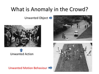
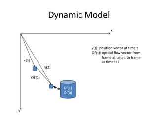
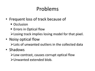
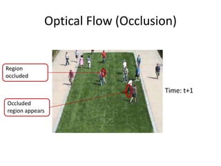
1. Detection
of
anomaly in human crowd
using
dynamic motion vector modeling
Abhishek Kumar
MASc., Video and Image Processing Lab
Supervisors: Profs. David Clausi and Paul Fieguth

2. Outline
• What is an anomaly in the crowd?
• Why do we anomaly detection?
• What is currently available?
• What do we want?
• How?
• My work
• Results.
• Conclusion

3. What is Anomaly in the Crowd?
Unwanted Object
Unwanted Action
Unwanted Motion Behaviour

4. Why do we need Anomaly detection?
• Avoid any hazardous situation
• Catch rule breakers
• Fix system problems which may lead to
greater problem

5. What is currently available?
 A couple of
surveillance
operator
keeps vigil on
a set of
monitors.
• Limitations:
• Monotonous
• Privacy issues
• Prone to Human
error

6. What do we want?

7. Methods of motion detection
• Frame difference
• Template matching
• Tracking
• Optical flow

8. Optical Flow
Time: t

9. Optical Flow
Time: t+1

10. Optical Flow
Time: t
Time: t+1

11. Algorithm of anomaly detection:
Start Frame(0) Frame(t)
Motion Parameters, i.e.
Optical Flow (t-1, t)
Motion
Model
Localized Outlier
detection for Current
Frame
Validation of outliers
Is
Verified
Alarm
t = t+1
t=1

12. Possible strategies of motion model
1. Model motion vector for a fixed pixel (static
model)
 Advantage: easier to model
 Disadvantage: May not do well in fast changing
crowd.
2. Model motion vector for trajectory of a fixed
point (dynamic model)
 Advantage: Can be very effective for changing crowd.
 Disadvantage: Difficult to model

13. Dynamic Model
Of(0)
x
y
v(0)
OF(0)v(1)
v(t): position vector at time t
OF(t): optical flow vector from
frame at time t to frame
at time t+1

14. Dynamic Model
Of(1)
Of(0)
x
y
v(2)
OF(1)
v(1)
v(t): position vector at time t
OF(t): optical flow vector from
frame at time t to frame
at time t+1

15. Dynamic Model
Of(2)
Of(1)
Of(0)
x
y
v(2)
OF(2)
v(3)
v(t): position vector at time t
OF(t): optical flow vector from
frame at time t to frame
at time t+1

16. Flow Mapping
• Pixels are quantized but motion vectors are
not.
• Ex. OF Vector: (x =3.3, y = 2.6)
• Just rounding looses information.
• Probabilistic mapping, 0.4*0.7 0.4*0.3
0.6*0.7 0.6*0.3
(2.6, 3.3)

17. Mapping (rounding based)
Three color channels
Green: OF based second
image
Blue: Second image
Red: missing OF based
Mapping.

18. Mapping (Probability based)
Three color channels
Green: OF based second
image
Blue: Second image
Red: missing OF based
Mapping.

19. Problems
• Frequent loss of track because of
 Occlusion
 Errors in Optical flow
Losing track implies losing model for that pixel.
• Noisy optical flow
Lots of unwanted outliers in the collected data
• Shadows
Low contrast, causes corrupt optical flow
Unwanted extended blob.

20. Optical Flow (Occlusion)
Time: t

21. Optical Flow (Occlusion)
Time: t+1

22. Optical Flow (Occlusion)
Time: t+1
Occluded
region appears
Region
occluded

23. Example (Anomaly situation)
Frame 457 Frame 499

24. Example
Frame 463 Frame 505

25. Example (Number of data)
Frame 463 Frame 505
Buffer size: 30
Data stored:
•Magnitude of flow Vector
•Angle of flow vector

26. Example (Segmented on motion
model)
Frame 463 Frame 505
Assumption of Normal Model
Closing operation on pixels with probability > 0.05

27. Example (Few trails)
Frame 463 Frame 505

28. Example : Flow magnitude and angle
Frame 463 Frame 505
Flowmagnitude
Flowmagnitude
Anglemagnitude
Anglemagnitude

29. What next?
• Given current situation, we are still trying to
find out ways to extract useful information out
of this model.
• To make this system robust against noise and
local variations, we can think of doing similar
modeling on larger homogenous regions.

30. Questions?