Downloaded 1,091 times


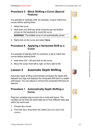
![Schlumberger Internal Use Only Basics of the Techlog Window
Techlog Fundamentals, Version 2012 41
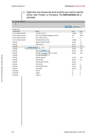
©2011-2013Schlumberger.Allrightsreserved.
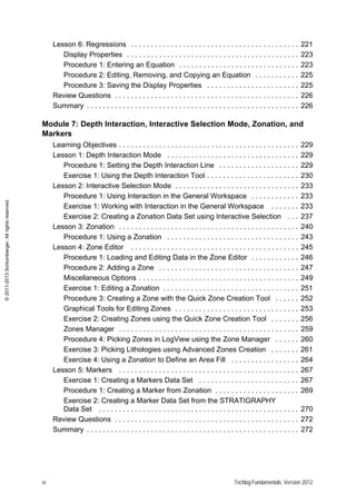
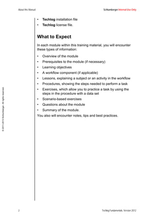
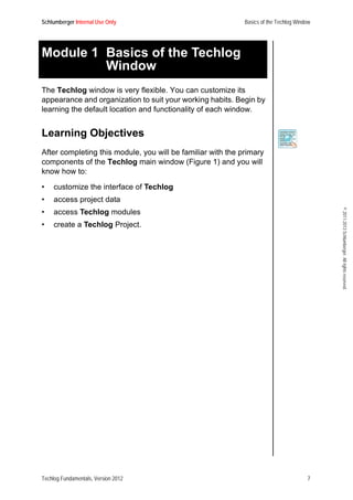
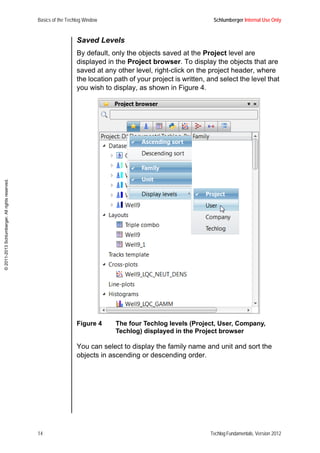
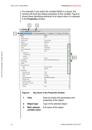
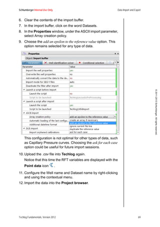
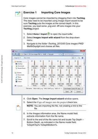
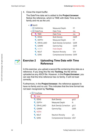
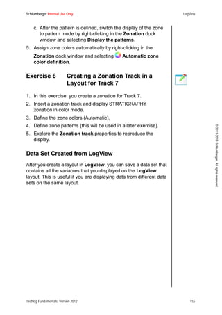
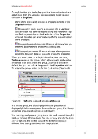
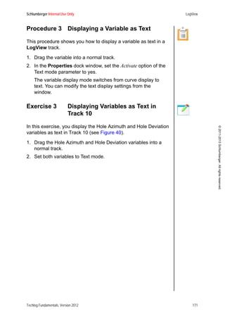
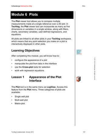
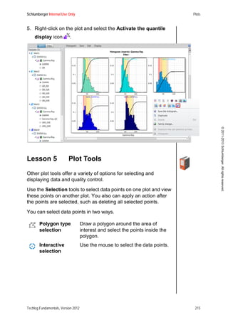
3. Click Next.
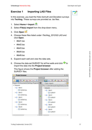
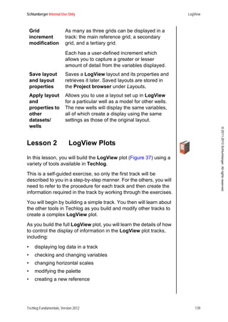
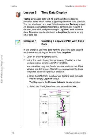
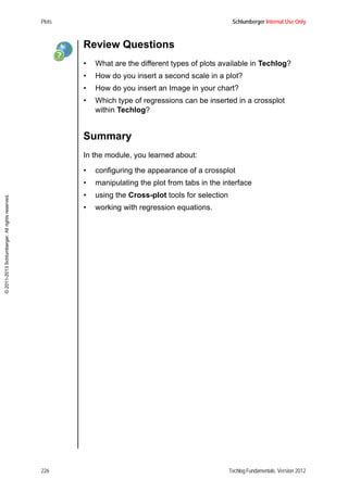
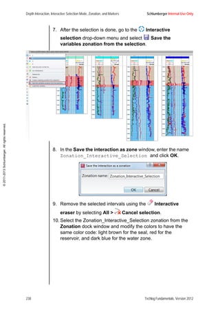
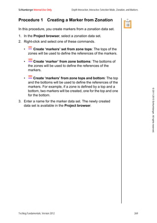
The Folder, status and type window opens. In this window,
you can modify the storage path for your project. For this
exercise, use these values:
• Project status: In progress
• Project opening default mode: single user [read/write]
• Project plug-in: SQlite
• Unit system: Undefined (for the moment, no company folder
is installed).
4. Click Next.
A confirmation dialog box opens asking you to confirm the
project folder creation.
5. Click Create.
Techlog creates the new project folder.](https://image.slidesharecdn.com/techlog2012fundamentalso-151021083902-lva1-app6891/85/Manuel-Logiciel-Techlog-2012-55-320.jpg)


![Schlumberger Internal Use Only Data Import and Export
Techlog Fundamentals, Version 2012 93
©2011-2013Schlumberger.Allrightsreserved.
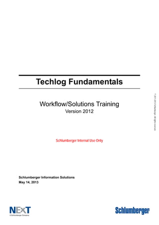
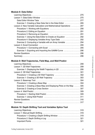
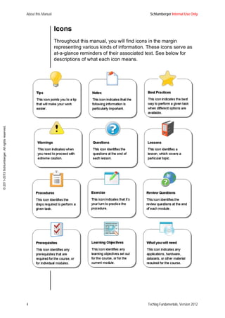
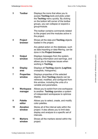
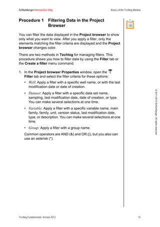
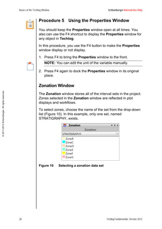
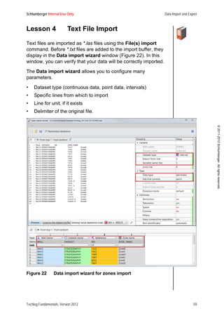
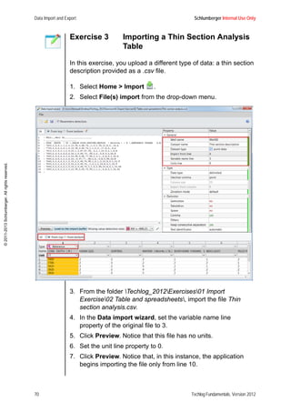
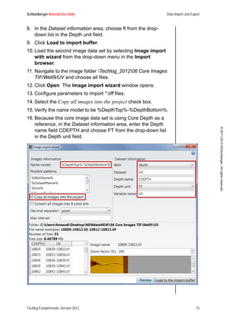
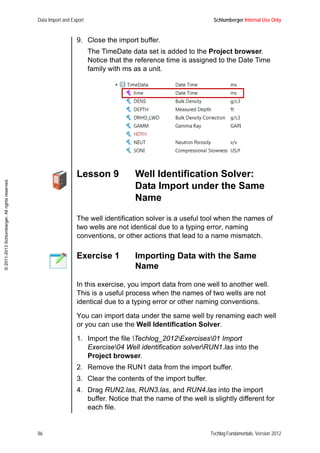
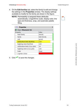
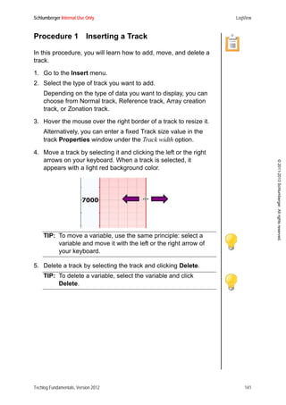
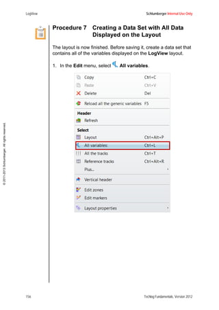
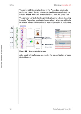
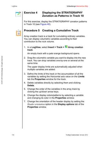
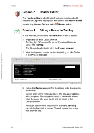
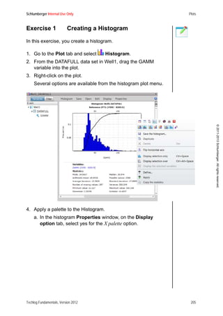
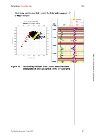
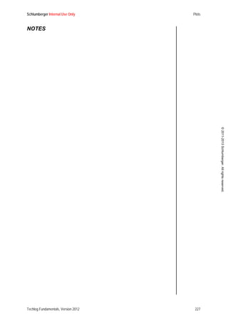
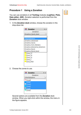
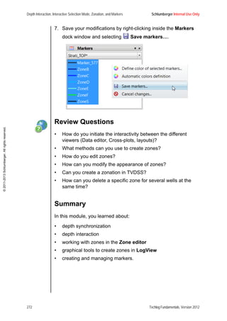
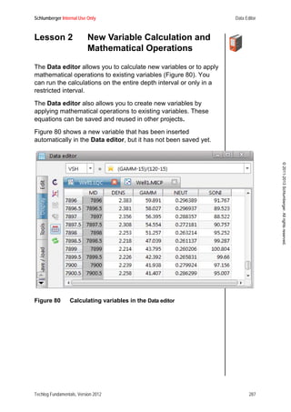
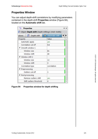
The new property now can be seen in the Properties
window. The modification has been made only for Well1.
10. Click Save .
11. Choose to export one file per data set using the automatic file
name WellName_DatasetName [LAS Certified].
12. Save the files on your desktop.
Techlog creates five files (one for each well).
13. Open the Well1_DATAFULL.las file and note the parameter
Interval Exported.](https://image.slidesharecdn.com/techlog2012fundamentalso-151021083902-lva1-app6891/85/Manuel-Logiciel-Techlog-2012-107-320.jpg)


![Data Editor Schlumberger Internal Use Only
294 Techlog Fundamentals, Version 2012
©2011-2013Schlumberger.Allrightsreserved.
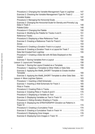
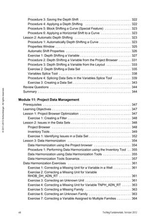
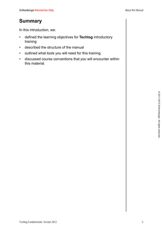
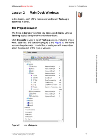
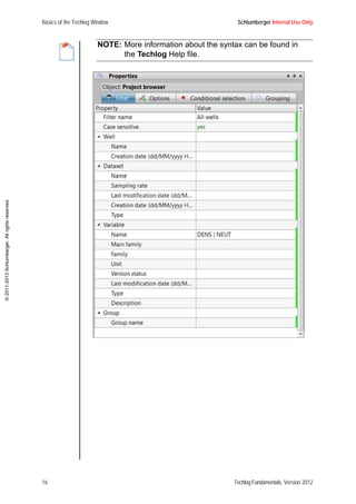
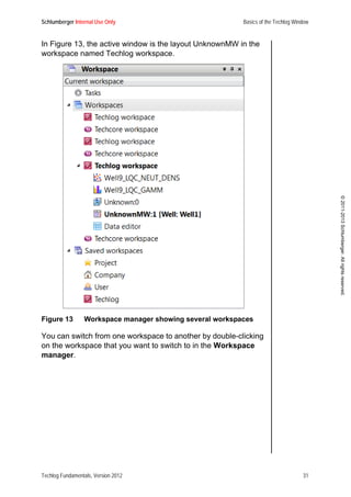
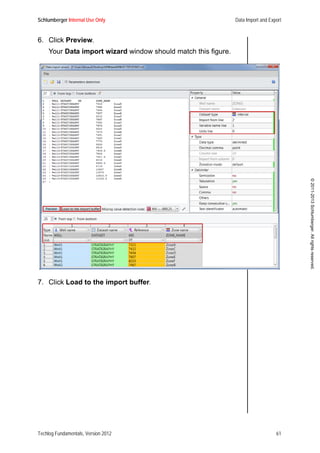
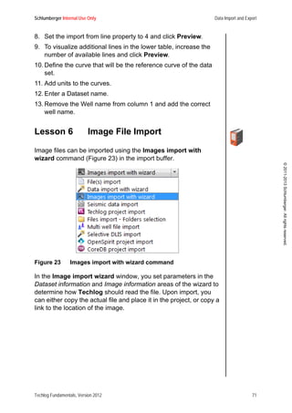
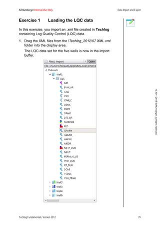
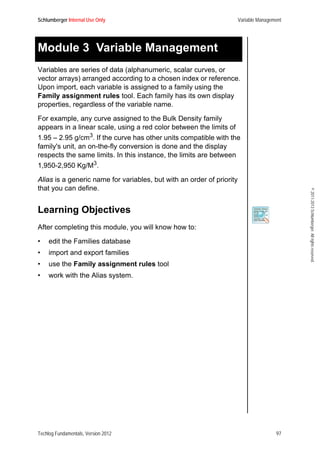
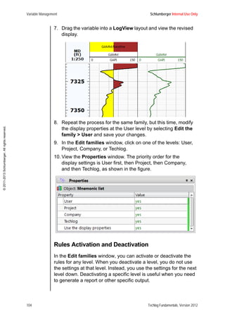
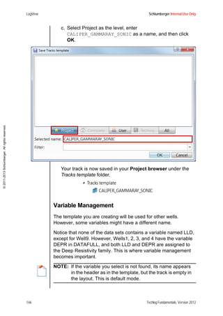
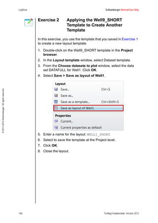
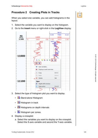
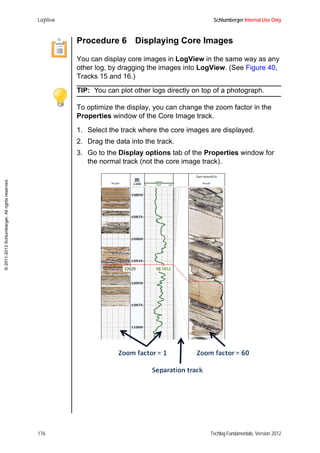
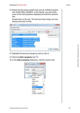
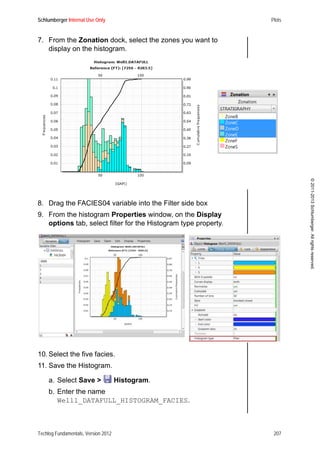
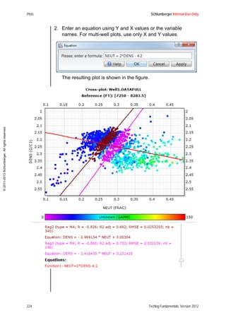
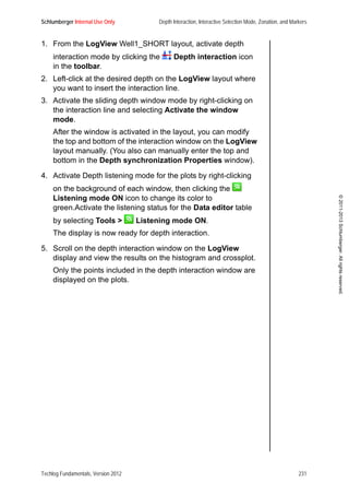
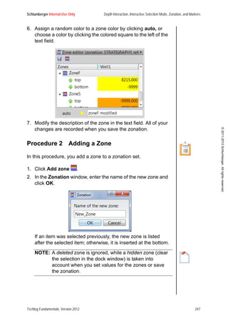
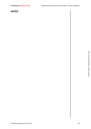
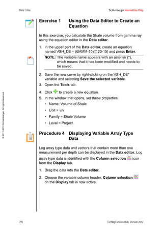
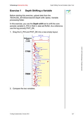
For example, if you multiply an array variable by a constant
value, all columns are multiplied by the same constant value.
The results are illustrated in the figure.
NOTE: The equation is defined with the name of the array
and the results are saved as an array variable.
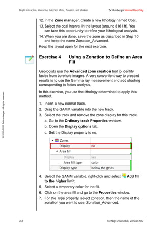
Exercise 2 Computing a Variable with an Array
Variable
In this exercise, you use log array type data in the Data editor to
compute a variable from an array variable.
1. Open a new empty Data editor.
2. Choose MICP from Well1.
3. Choose the array CShg.
4. Drag the array into the Data editor.
5. Select the CShg column.
6. On the Display tab, click .
7. Choose several column numbers and click OK.
8. In the equation area, compute CSW as 1-CShg.
Notice that the Data editor displays only the first column of
the computed array.
9. Select CSW[0] and click to select the columns to display.
10. Choose the new variables and click .](https://image.slidesharecdn.com/techlog2012fundamentalso-151021083902-lva1-app6891/85/Manuel-Logiciel-Techlog-2012-308-320.jpg)


![Project Data Management Schlumberger Internal Use Only
362 Techlog Fundamentals, Version 2012
©2011-2013Schlumberger.Allrightsreserved.
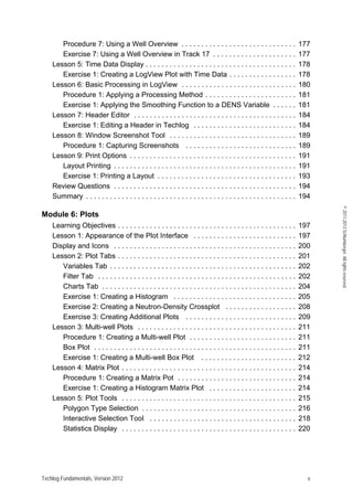
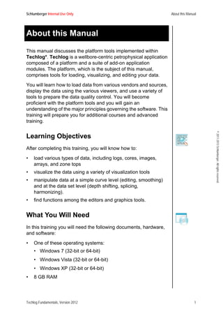
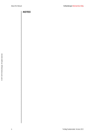
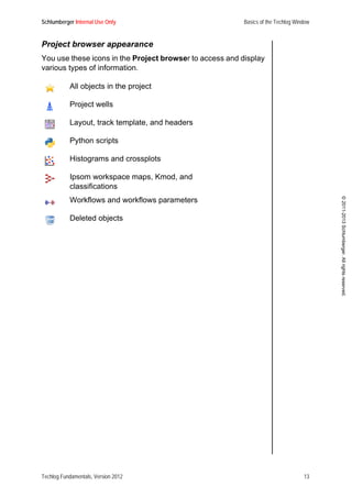
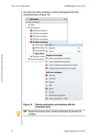
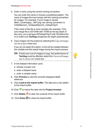
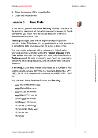
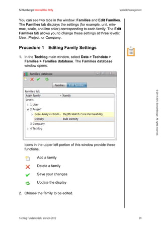
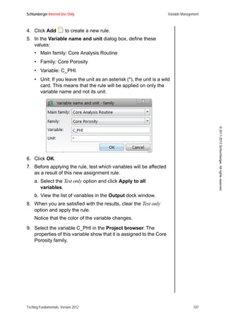
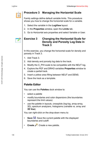
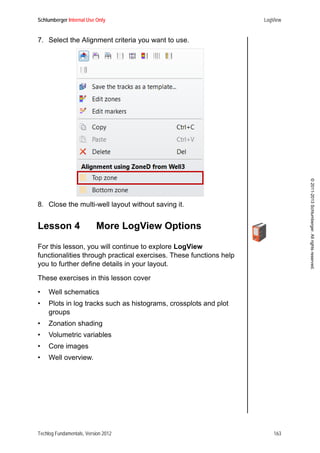
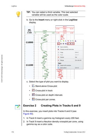
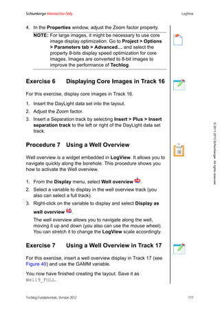
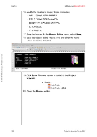
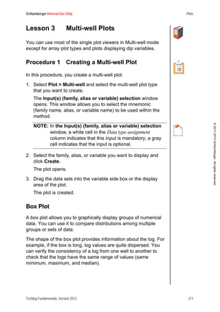
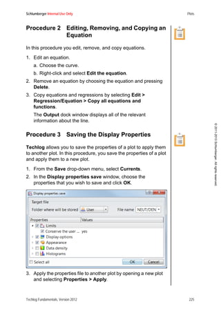
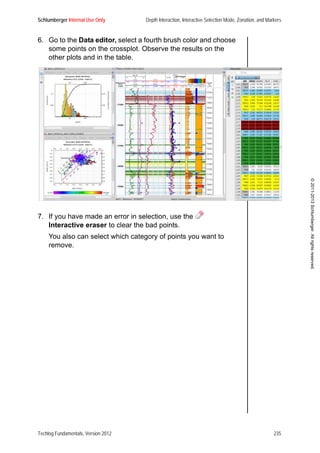
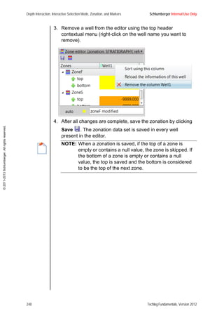
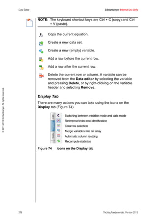
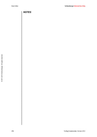
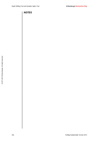
4. Set the After field to ohm.m.
5. Set a variable filter to RT.
6. Click Preview and click Rename.
7. Repeat the same operation for the variables RW.
TIP: A quicker way to do this is to create a conditional
selection in your Project browser on RT and RW, then
apply a filter. Then you can use the Query rename tool
to change the unit.
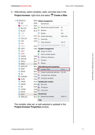
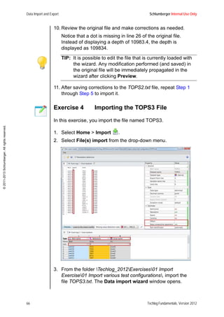
An alternate method is to write a filter in the Properties
window of the Query rename tool. In the Properties
window, you can select two types of expression: basic (DOS)
and complex (UNIX/Perl).
For this example you can select complex and insert R[T|W]
in the Filter section in the Variable field. All syntax
expressions are available in the Techlog Help file. RT and
RW variables will be selected automatically.](https://image.slidesharecdn.com/techlog2012fundamentalso-151021083902-lva1-app6891/85/Manuel-Logiciel-Techlog-2012-376-320.jpg)


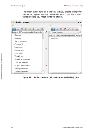
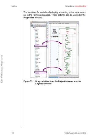
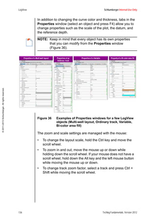
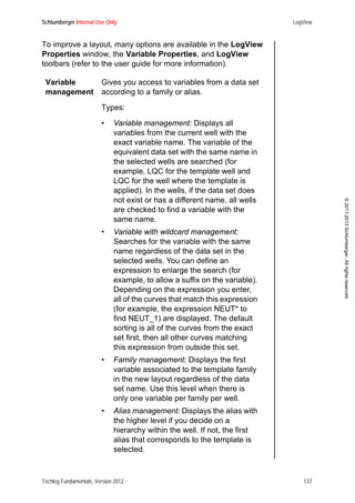
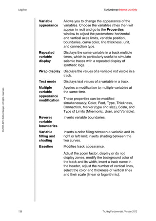
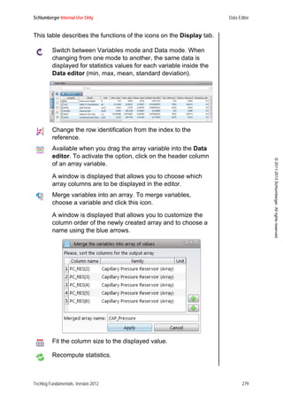
This document provides an overview and instructions for using Schlumberger's Techlog software. It covers the main components of the Techlog window, how to create and open Techlog projects, import and export data in various file formats, and manage variables through families. The document is copyrighted and its use is governed by Schlumberger's license agreement.