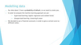
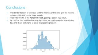
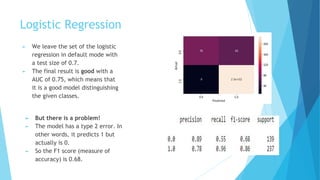
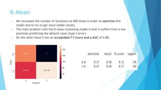
1) The document discusses using machine learning techniques like logistic regression, random forest, and K-means clustering to develop a credit scoring model based on financial ratios to predict a company's probability of default. 2) Random forest performed the best with an AUC of 0.87 and high precision and recall, while logistic regression had a AUC of 0.75 but issues with type II errors. 3) K-means clustering had a lower precision predicting defaults but an acceptable F1-score and AUC of 0.80.

1. Machine Learning Application:
Credit Scoring
Programming Techniques
Professor Carlos Costa
Master in Mathematical Finance
Federico Innocenti 53251
Miguel Albergaria 48547
Claudio Napoli 53358
Iacopo Fiorentino 53315 Lisbon, December 11th
2019

2. Context
► The data is collected from Thomson Reuters from firms
included in the main stock indexes.
► The goal is to set a score of a company to decide
whether to give a loan or not to that firm based on a
client’s probability of default.
► For that we compute many ratios and at the end we
want to “differentiate winners from losers”.

3. Data preparation
► Importing data, checking the type of data and
clearing missing values;
► Correlation matrix;
► See how the data is distributed through graphs;
► Rearranging the data clearing very low values
and very high values, i.e., outliers.
► After all of that, we did the correlation matrix
and graphs again to compare them and to have
a better view of our results.

4. Modelling data
► Our data doesn´t have a probability of default, so we need to create one.
► In order to compute the machine learning approach we use:
► Supervised learning: logistic regression and random forest
► Unsupervised learning: clustering K-mean
► We decided to use a financial scorecard, in order to give a certain score to
different ratios.

5. Setting the score
► Relevant ratios: current ratio, debt ratio, equity to asset ratio, debt to
equity ratio, return on asset, return on equity, long term coverage ratio and
asset turnover ratio.

6. ► The company’s goal is to obtain the highest score that we compute in the
way showed before. An example of the code is shown here:
► The final score is set by adding all of the “ratios’ scores”.

7. Evaluation
► For the evaluation of our model we compute a confusion matrix in order to
see the result and have an easier first parametre to compare the three
models.
► After setting the score we binarize the score being 1 the lowest probability
of default and 0 the highest. We chose as threshold a score of 500 points and
then we proceed to the evaluation.

8. Logistic Regression
► We leave the set of the logistic
regression in default mode with
a test size of 0.7.
► The final result is good with a
AUC of 0.75, which means that
it is a good model distinguishing
the given classes.
► But there is a problem!
► The model has a type 2 error. In
other words, it predicts 1 but
actually is 0.
► So the F1 score (measure of
accuracy) is 0.68.

9. Random Forest
► In order to optimize the process we put the “number of jobs” 150 and the
“number of estimators” is 1 since it is a binomial classification.

10. ► This model achieved a really high AUC: 0.87 and a good F1-Score.
► High precision and high recall means low probability of error type I and II.

11. K-Mean
► We increased the number of iterations to 400 times in order to optimize this
model and to try to get more stable results.
► The main problem with the K-mean clustering model is that it suffers from a low
precision predicting the default cases (type I error).
► On the other hand it has an acceptable F1-Score and a AUC of 0.80.

12. Conclusions
► The standardization of the ratio and the cleaning of the data gets the models
to have a high AUC on the three models.
► The better model is the Random Forest, getting a better AUC result.
► We confirm that machine learning algorithms are really powerful in analysing
data and it can be helpful to solve this specific problem.