The document provides an overview of Bayesian learning and reasoning in machine learning, highlighting the significance of Bayesian algorithms in handling probability distributions and decision making. It discusses key concepts such as Bayes' theorem, maximum likelihood hypothesis, and naive Bayes classifier, along with their features, limitations, and practical applications, including medical diagnosis examples. Additionally, it covers advanced topics like Gibbs sampling and Bayesian belief networks to infer dependencies among variables.

1. 1
Bayesian Learning
Bayesian Learning
Machine Learning
Chapter 6
발표자 : 김 석 준

2. 2
Bayesian Reasoning
Bayesian Reasoning
• Basic assumption
– The quantities of interest are governed by probability distri
bution
– These probability + observed data ==> reasoning ==> opti
mal decision
• 의의 , 중요성
– 직접적으로 확률을 다루는 알고리듬의 근간
• 예 ) naïve Bayes classifier
– 확률을 다루지 않는 알고리듬을 분석하기 위한 틀
• 예 ) cross entropy , Inductive bias decision tree, MDL principle

3. 3
Feature & Limitation
Feature & Limitation
• Feature of Bayesian Learning
– 관측된 데이터들은 추정된 확률을 점진적으로 증감
– Prior Knowledge : P(h) , P(D|h)
– Probabilistic Prediction 에 응용
– multiple hypothesis 의 결합에 의한 prediction
• 문제점
– initial knowledge 요구
– significant computational cost

4. 4
Bayes Theorem
Bayes Theorem
• Terms
– P(h) : prior probability of h
– P(D) : prior probability that D will be observed
– P(D|h) : prior knowledge
– P(h|D) : posterior probability of h , given D
• Theorem
• machine learning : 주어진 데이터 들로부터 the
most probable hypothesis 를 찾는 과정
)
(
)
(
)
|
(
)
|
(
D
P
h
P
h
D
P
D
h
P 

5. 5
Example
Example
• Medical diagnosis
– P(cancer)=0.008 , P(~cancer)=0.992
– P(+|cancer) = 0.98 , P(-|cancer) = 0.02
– P(+|~cancer) = 0.03 , P(-|~cancer) = 0.97
– P(cancer|+) = P(+|cancer)P(cancer) = 0.0078
– P(~cancer|+) = P(+|~cancer)P(~cancer) = 0.0298
– hMAP = ~cancer

6. 6
MAP hypothesis
MAP hypothesis
MAP(Maximum a posteriori) hypothesis
)
(
)
|
(
max
arg
)
(
)
(
)
|
(
max
arg
)
|
(
max
arg
h
P
h
D
P
D
P
h
P
h
D
P
D
h
P
h
H
h
h
H
h
MAP





)
(
)
|
(
max
arg h
P
h
D
P
h
H
h
MAP



7. 7
ML hypothesis
ML hypothesis
• maximum likelihood (ML) hypothesis
– basic assumption : equally probable a priori
• basic formular
– P(a^b) = P(A|B)P(B) = P(B|A)P(A)
)
|
(
max
arg h
D
P
h
H
h
ML




i
i
i A
P
A
B
P
B
P )
(
)
|
(
)
(

8. 8
Bayes Theorem and Concept Lea
Bayes Theorem and Concept Lea
rning
rning
• Brute-force MAP learning
– for each calculate P(h|D)
– find hMAP
• consistent assumption
– noise free data D
– target concept c in hypothesis space H
– every hypothesis is equally probable
• Result
• every consistent hypothesis is MAP hypothesis
D
H
VS
D
h
P
,
1
)
|
(  (if h is consistent with D)
P(h|D) = 0 (otherwise)

9. H
VS
H
h
P
x
h
h
D
P
H
h
P
D
H
VS
h
H
h
i
i
D
H
i
i
,
i
i
,
1
1
)
(
)
h
|
P(D
P(D)
0
else
,
)
(
d
if
1
)
|
(
1
)
(










D
H
D
H
VS
VS
H
H
D
P
h
P
D
P
h
P
h
D
P
D
h
P
,
,
1
1
)
(
)
(
1
)
(
)
(
)
|
(
)
|
(






10. 10
Consistent learner
Consistent learner
• 정의 : training example 들에 대해 에러가 없는
hypothesis 를 출력해 주는 알고리듬
• result :
– every consistent hypothesis output == MAP hypothesis
– every consistent learner output == MAP hypothesis
• if uniform prior probability distribution over H
• if deterministic, noise-free training data

11. 11
ML and LSE hypothesis
ML and LSE hypothesis
• Least squared error hypothesis
– NN , curve fitting, linear regression
– continuous-valued target function
• task : find f : di=f(xi)+ei
• preliminary :
– probability densities, Normal distribution
– target value independence
• result :
• limitation : noise only in the target value





m
i
i
i
H
h
ML x
h
d
h
1
2
))
(
(
min
arg

12. 














2
2
2
2
2
))
(
(
2
1
2
))
(
(
2
1
min
arg
))
(
(
2
1
2
1
ln
max
arg
2
1
max
arg
)
|
(
max
arg
)
|
(
max
arg
2
2
i
i
h
i
i
h
x
h
d
h
m
i
i
h
H
h
ML
x
h
d
x
h
d
e
h
d
P
h
D
P
h
i
i






13. 13
ML hypothesis for predicting
ML hypothesis for predicting
Probability
Probability
• Task : find g : g(x) = P(f(x)=1)
• question : what criterion should we optimize in
order to find a ML hypothesis for g
• result : cross entropy
– entropy function :







m
i
i
i
i
i
H
h
ML x
h
d
x
h
d
h
1
))
(
1
ln(
)
1
(
)
(
ln
max
arg


i
i
i P
P ln

14. 



)
(
)
,
|
(
)
|
,
(
)
|
(
i
i
i
m
i
i
i
x
P
x
h
d
P
h
d
x
P
h
D
P
i
i d
i
d
i
i
i
i
i
i
i
i
i
x
h
x
h
x
h
d
P
x
h
x
h
d
P
x
h
x
h
d
P









1
i
i
))
(
1
(
)
(
)
,
|
(
0
d
if
,
)
(
1
)
,
|
(
1
d
if
,
)
(
)
,
|
(
 














))
(
1
ln(
)
1
(
)
(
ln
max
arg
))
(
1
(
)
(
max
arg
)
(
))
(
1
(
)
(
max
arg
)
|
(
max
arg
1
1
i
i
i
i
h
d
i
d
i
h
i
d
i
d
i
h
h
ML
x
h
d
x
h
d
x
h
x
h
x
p
x
h
x
h
h
D
P
h
i
i
i
i

15. 15
Gradient search to ML in NN
Gradient search to ML in NN
Let G(h,D) = cross entropy
jk
jk
D
h
G
w






)
,
(





m
i
ijk
i
i
jk x
x
h
d
w
1
))
(
(







m
i
ijk
i
i
i
i
jk x
x
h
d
x
h
x
h
w
1
))
(
))(
(
1
)(
(
 (BP)
By gradient ascent

16. 


































ijk
i
i
ijk
i
i
i
i
i
i
jk
i
i
i
i
i
jk
i
i
i
i
i
i
jk
i
i
jk
i
i
i
i
x
x
h
d
x
x
h
x
h
x
h
x
h
x
h
d
w
x
h
x
h
x
h
x
h
d
w
x
h
x
h
x
h
d
x
h
d
w
x
h
x
h
D
h
G
w
D
h
G
x
h
d
x
h
d
let
))
(
(
1
))
(
1
)(
(
))
(
1
)(
(
)
(
)
(
))
(
1
)(
(
)
(
)
(
)
(
)))
(
1
ln(
)
1
(
)
(
ln
(
)
(
)
(
)
,
(
)
,
(
))
(
1
ln(
)
1
(
)
(
ln
D)
G(h,
jk
jk
D
h
G
w






)
,
(

17. 17
MDL principle
MDL principle
• 목적 : Bayesian method 에 의한 inductive bias
와 MLD principle 해석
• Shannon and weaver’s optimal code length
))
(
log
)
|
(
log
(
min
arg
))
(
log
)
|
(
(log
max
arg
2
2
2
2
h
P
h
D
P
h
P
h
D
P
h
H
h
H
h
MAP







)
|
(
)
(
min
arg |
h
D
L
h
L
h H
D
H C
C
H
h
MAP 


)
|
(
)
(
min
arg 2
1
h
D
L
h
L
h C
C
H
h
MDL 


(bits)
log2 i
P


18. 18
Bayes optimal classifier
Bayes optimal classifier
• Motivation : 새로운 instance 의 classification 은 모든 hypot
hesis 에 의한 prediction 의 결합으로 인하여 최적화
되어진다 .
• task : Find the most probable classification of the new instance g
iven the training data
• answer :combining the prediction of all hypotheses
• Bayes optimal classification
• limitation : significant computational cost ==> Gibbs algorithm


 V
v
i
i
j
V
v
i
j
D
h
P
h
v
P )
|
(
)
|
(
max
arg

19. 19
Bayes optimal classifier example
Bayes optimal classifier example
0
)
h
|
P(
1
)
h
|
P(-
3
.
)
|
(
0
)
h
|
P(
1
)
h
|
P(-
3
.
)
|
(
1
)
h
|
P(
0
)
h
|
P(-
4
.
)
|
(
3
3
3
2
2
2
1
1
1












D
h
P
D
h
P
D
h
P















H
h
i
i
j
v
H
h
i
i
H
h
i
i
i
j
i
i
D
h
P
h
v
P
D
h
P
h
P
D
h
P
h
P
)
|
(
)
|
(
max
arg
6
.
)
|
(
)
|
(
4
.
)
|
(
)
|
(
}
,
{

20. 20
Gibbs algorithm
Gibbs algorithm
• Algorithm
– 1. Choose h from H, according to the posterior probabil
ity distribution over H
– 2. Use h to predict the classification of x
• Gibbs algorithm 의 유용성
– Haussler , 1994
– Error(Gibbs algorithm)< 2*Error(Bayes optimal classifi
er)

21. 21
Naïve Bayes classifier
Naïve Bayes classifier
• Naïve Bayes classifier
• difference
– no explicit search through H
– by counting the frequency of existing examples
• m-estimate of probability =
– m : equivalent sample size , p : prior estimate of probability
)
(
)
|
,...,
,
(
max
arg 2
1 j
j
n
MAP v
P
v
a
a
a
P
v 



i
j
i
j
V
v
NB v
a
p
v
P
v
j
)
|
(
)
(
max
arg
m
n
mp
nc



22. 22
example
example
• (outlook=sunny,temperature=cool,humidity=high,wind=str
ong)
• P(wind=strong|playTennis=yes)=3/9=.33
• P(wind=string|PlayTennis=no)=3/5=.60
• P(yes)P(sunny|yes)P(cool|yes)P(high|yes)P(strong|yes)=.0
053
• P(no)P(sunny|no)P(cool|no)P(high|no)P(strong|no)=.0206
• vNB = no

23. 23
Bayes Belief Networks
Bayes Belief Networks
• 정의
– describe the joint probability distribution for a set of variables
– 모든 변수들이 conditional independence 일것을 요구하지 않음
– 변수들간의 부분적 의존 관계를 확률로 표현
• representation

24. 24
Bayesian Belief Networks
Bayesian Belief Networks

25. 25
Inference
Inference
• Task : infer the probability distribution for
the target variables
• methods
– exact inference : NP hard
– approximate inference
• theoretically NP hard
• practically useful
• Monte Carlo methods

26. 26
Learning
Learning
• Env
– structure known + fully observable data
• easy , by naïve Bayes classifier
– structure known + partially observable data
• gradient ascent procedure ( by Russel , 1995 )
• ML hypothesis 와 유사 P(D|h)
– structure unknown




D
d ijk
ik
ij
h
ijk
ijk
w
d
u
y
P
w
w
)
|
,
(


27. 27
Learning(2)
Learning(2)
• Structure unknown
– Bayesian scoring metric ( cooper, Herskovits, 1992 )
– K2 algorithm
• cooper, Herskovits, 1992
• heuristic greedy search
• fully observed data
– constraint-based approach
• Spirtes, 1993
• infer dependency and independency relationship
• construct structure using this relationship

28. 




D
d ijk
ik
ij
h
ijk
ijk
w
d
u
y
P
w
w
)
|
,
(

 
 




















'
,
'
'
'
'
'
'
'
,
'
'
'
'
'
)
(
)
|
(
)
,
|
(
)
(
1
)
,
(
)
,
|
(
)
(
1
)
(
ln
)
(
1
)
(
ln
)
(
ln
)
(
ln
k
j
ik
ik
ij
h
ik
ij
h
ijk
h
k
j
ik
ij
h
ik
ij
h
ijk
h
d ijk
h
h
d
h
ijk
d
h
ijk
ijk
h
u
P
u
y
P
u
y
d
P
w
d
P
u
y
P
u
y
d
P
w
d
P
w
d
P
d
P
d
P
w
D
P
w
w
D
P














ijk
ik
ij
h
ik
ij
h
ik
ij
h
ik
ij
h
ik
ik
ij
h
ik
ij
h
ik
h
ik
ij
h
h
ik
ik
ij
h
h
ik
ik
ij
h
ik
ij
h
ijk
h
w
d
u
y
P
u
y
P
d
u
y
P
u
y
P
u
P
d
u
y
P
u
y
P
u
P
d
P
d
u
y
P
d
P
u
P
u
y
d
P
d
P
u
P
u
y
P
u
y
d
P
w
d
P
)
|
,
(
)
|
(
)
|
,
(
)
,
(
)
(
)
|
,
(
)
,
(
)
(
)
(
)
|
,
(
)
(
1
)
(
)
,
|
(
)
(
1
)
(
)
|
(
)
,
|
(
)
(
1
0
w
else
0
w
then
)
k
k'
,
'
(
)
|
(
ijk
ijk









i
i
if
u
y
P
w ik
ij
h
ijk

29. 29
EM algorithm
EM algorithm
• EM : estimation, maximization
• env
– learning in the presence of unobserved variables
– the form of probability distribution is known
• application
– training Bayesian belief networks
– training radial basis function networks
– basis for many unsupervised clustering algorithm
– basis for Baum-Welch’s forward-backward algorithm

30. 30
K-means algorithm
K-means algorithm
• Env : k normal distribution 들로부터 임의로 dat
a 생성
• task : find mean values of each distribution
• instance : < xi,z11,z12>
– if z is known : using
– else use EM algorithm
i
i
ML x
 
 2
)
(
min
arg 


31. 31
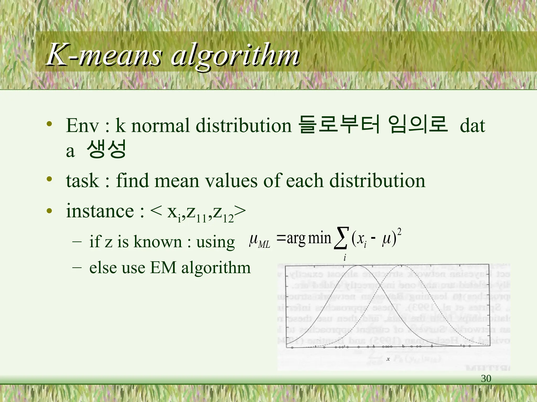
K-means algorithm
K-means algorithm
• Initialize
• calculate E[z]
• calculate a new ML hypothesis

 




 2
2
2
2
)
(
2
1
)
(
2
1
)
|
(
)
|
(
]
[
k
i
j
i
x
x
k
k
i
j
i
ij
e
e
x
P
x
P
z
E









m
i
i
ij
j x
z
E
m 1
]
[
1

==> converge to a local ML hypothesis

32. 32
General statement of EM algo
General statement of EM algo
• Terms
  : underlying probability distribution
– x : observed data from each distribution
– z : unobserved data
– Y = X union Z
– h : current hypothesis of 
– h’ : revised hypothesis
• task : estimate  from X

33. 33
guideline
guideline
• Search h’
• if h =  : calculate function Q
)]
|
(
[ln
max
arg h
Y
P
E
h
h




]
,
|
)
|
(
[ln
)
|
( X
h
h
Y
P
E
h
h
Q 



34. 34
EM algorithm
EM algorithm
• Estimation step
• maximization step
• converge to a local maxima
]
,
|
)
|
(
[ln
)
|
( X
h
h
Y
P
E
h
h
Q 


)
|
(
max
arg h
h
Q
h
h




35. 




k
j
j
i
ij x
Z
ik
i
i
i
i
e
h
z
z
z
x
P
h
y
P
2
'
2
)
(
2
1
2
2
1
2
1
)
'
|
,...,
,
,
(
)
'
|
(



 







)
)
(
2
1
2
1
(ln
)
'
|
(
ln
)
'
|
(
ln
)
'
|
(
ln
2
'
2
2 j
i
ij
i
i
x
Z
h
y
P
h
y
P
h
Y
P



)
|
(
)
](
[
2
1
2
1
ln
]
)
)
(
2
1
2
1
(ln
[
)]
'
|
(
[ln
'
2
'
2
2
2
'
2
2
h
h
Q
x
Z
E
x
Z
E
h
Y
P
E
m
i
j
i
ij
j
i
ij















 
 







 




 2
2
2
2
)
(
2
1
)
(
2
1
)
|
(
)
|
(
]
[
k
i
j
i
x
x
k
k
i
j
i
ij
e
e
x
P
x
P
z
E









m
i
i
ij
j x
z
E
m 1
]
[
1
