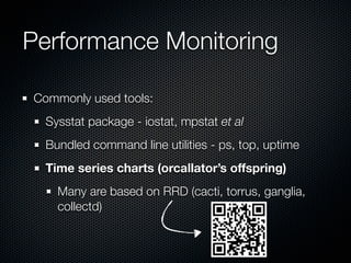
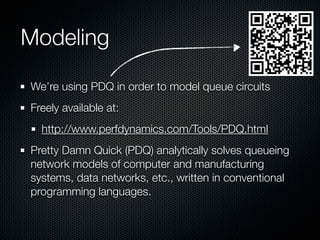
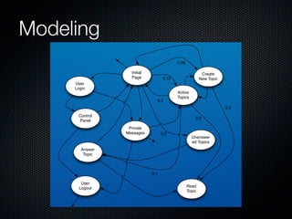
Linux Systems Capacity
Planning
Rodrigo Campos
camposr@gmail.com - @xinu
USENIX LISA ’11 - Boston, MA
Agenda
Where, what, why?
Performance monitoring
Capacity Planning
Putting it all together
Where, what, why ?
75 million internet users
1,419.6% growth (2000-2011)
29% increase in unique IPv4 addresses (2010-2011)
37% population penetration

Sources:
Internet World Stats - http://www.internetworldstats.com/stats15.htm
Akamai’s State of the Internet 2nd Quarter 2011 report - http://www.akamai.com/stateoftheinternet/
Where, what, why ?
High taxes
Shrinking budgets
High Infrastructure costs
Complicated (immature?) procurement processes
Lack of economically feasible hardware options
Lack of technically qualified professionals
Where, what, why ?
Do more with the same infrastructure
Move away from tactical fire fighting
While at it, handle:
Unpredicted traffic spikes
High demand events
Organic growth
Performance Monitoring
Typical system performance metrics
CPU usage
IO rates
Memory usage
Network traffic
Performance Monitoring
Commonly used tools:
Sysstat package - iostat, mpstat et al
Bundled command line utilities - ps, top, uptime
Time series charts (orcallator’s offspring)
Many are based on RRD (cacti, torrus, ganglia,
collectd)
Performance Monitoring
Time series performance data is useful for:
Troubleshooting
Simplistic forecasting
Find trends and seasonal behavior
Performance Monitoring
"Correlation does not imply causation"
Time series methods won’t help you much for:
Create what-if scenarios
Fully understand application behavior
Identify non obvious bottlenecks
Monitoring vs. Modeling
“The difference between performance
modeling and performance monitoring is
like the difference between weather
prediction and simply watching a weathervane twist in the wind”

Source: http://www,perfdynamics,com/Manifesto/gcaprules,html
Capacity Planning
Not exactly something new...
Can we apply the very same techniques to modern,
distributed systems ?
Should we ?
What’s in a queue ?
Agner Krarup Erlang
Invented the fields of traffic engineering and
queuing theory
1909 - Published “The theory of Probabilities
and Telephone Conversations”
What’s in a queue ?

Allan Scherr (1967) used the
machine repairman problem to
represent a timesharing system
with n terminals
What’s in a queue ?
Dr. Leonard Kleinrock
“Queueing Systems” (1975) - ISBN 0471491101
Created the basic principles of packet switching while
at MIT
What’s in a queue ?
(A)
Open/Closed
Network
A

Arrival Count

λ
W

Arrival Rate (A/T)
Time spent in Queue

R

Residence Time (W+S)

S

Service Time

X

System Throughput (C/T)

C

Completed tasks count

λ

S

W
R

X

(C)
Service Time
Time spent in processing (S)
Web server response time
Total Query time
Time spent in IO operation
System Throughput
Arrival rate (λ) and system throughput (X) are the same
in a steady queue system (i.e. stable queue size)
Hits per second
Queries per second
IOPS
Utilization
Utilization (ρ) is the amount of time that a queuing node
(e.g. a server) is busy (B) during the measurement
period (T)
Pretty simple, but helps us to get processor share of an
application using getrusage() output
Important when you have multicore systems

ρ = B/T
Utilization
CPU bound HPC application running in a two core
virtualized system
Every 10 seconds it prints resource utilization data to a
log file
Utilization
(void)getrusage(RUSAGE_SELF, &ru);
(void)printRusage(&ru);
...
static void printRusage(struct rusage *ru)
{
fprintf(stderr, "user time = %lfn",
(double)ru->ru_utime.tv_sec + (double)ru->ru_utime.tv_usec / 1000000);
fprintf(stderr, "system time = %lfn",
(double)ru->ru_stime.tv_sec + (double)ru->ru_stime.tv_usec / 1000000);
} // end of printRusage

10 seconds wallclock time
377,632 jobs done
user time = 7.028439
system time = 0.008000
Utilization
ρ = B/T

We have 2 cores so we
can run 3 application
instances in each server
(200/70.36) = 2.84

ρ = (7.028+0.008) / 10
ρ = 70.36%
Little’s Law
Named after MIT professor John Dutton Conant Little
The long-term average number of customers in a
stable system L is equal to the long-term average
effective arrival rate, λ, multiplied by the average time a
customer spends in the system, W; or expressed
algebraically: L = λW
You can use this to calculate the minimum
amount of spare workers in any application
Little’s Law
L = λW
λ = 120 hits/s

tcpdump -vttttt

W = Round-trip delay + service time
W = 0.01594 + 0.07834 = 0.09428
L = 120 * 0.09428 = 11,31
Utilization and Little’s Law
By substitution, we can get the utilization by multiplying
the arrival rate and the mean service time

ρ = λS
Putting it all together
Applications write in a log file the service time and
throughput for most operations
For Apache:
%D in mod_log_config (microseconds)
“ExtendedStatus On” whenever it’s possible
For nginx:
$request_time in HttpLogModule (milliseconds)
Putting it all together

Generated with HPA: https://github.com/camposr/HTTP-Performance-Analyzer
Putting it all together
A simple tag collection data store
For each data operation:
A 64 bit counter for the number of calls
An average counter for the service time
Putting it all together
Method

Call Count

Service Time (ms)

dbConnect

1,876

11.2

fetchDatum

19,987,182

12.4

postDatum

1,285,765

98.4

deleteDatum

312,873

31.1

fetchKeys

27,334,983

278.3

fetchCollection

34,873,194

211.9

createCollection

118,853

219.4
Putting it all together
Call Count x Service Time

fetchKeys

Service Time (ms)

createCollection
fetchCollection

deleteDatum

postDatum
dbConnect

fetchDatum
Call Count
Modeling
An abstraction of a complex system
Allows us to observe phenomena that can not be easily
replicated
“Models come from God, data comes from the devil” Neil Gunther, PhD.
Modeling
Clients

Requests

Web Server

Replies

Application

Database
Modeling
Clients

Requests

Cache

Replies

Web Server

Application

Database
Modeling
We’re using PDQ in order to model queue circuits
Freely available at:
http://www.perfdynamics.com/Tools/PDQ.html
Pretty Damn Quick (PDQ) analytically solves queueing
network models of computer and manufacturing
systems, data networks, etc., written in conventional
programming languages.
Modeling
CreateNode()

Define a queuing center

CreateOpen()

Define a traffic stream of an
open circuit

CreateClosed()

Define a traffic stream of a
closed circuit

SetDemand()

Define the service demand for
each of the queuing centers
Modeling
$httpServiceTime = 0.00019;
$appServiceTime = 0.0012;
$dbServiceTime = 0.00099;
$arrivalRate = 18.762;
pdq::Init("Tag Service");
$pdq::nodes = pdq::CreateNode('HTTP Server',
$pdq::CEN, $pdq::FCFS);
$pdq::nodes = pdq::CreateNode('Application Server',
$pdq::CEN, $pdq::FCFS);
$pdq::nodes = pdq::CreateNode('Database Server',
$pdq::CEN, $pdq::FCFS);
Modeling
=======================================
******
PDQ Model OUTPUTS
*******
=======================================
Solution Method: CANON
******

SYSTEM Performance
Value
-----

*******

Metric
-----Workload: "Application"
Number in system
Mean throughput
Response time
Stretch factor

Unit
----

1.3379
18.7620
0.0713
1.5970

Requests
Requests/Seconds
Seconds

Bounds Analysis:
Max throughput
Min response

44.4160
0.0447

Requests/Seconds
Seconds
0.0
009
8"
0.0
010
3"
0.0
010
8"
0.0
011
3"
0.0
011
8"
0.0
012
3"
0.0
012
8"
0.0
013
3"
0.0
013
8"
0.0
014
3"
0.0
014
8"
0.0
015
3"
0.0
015
8"
0.0
016
3"
0.0
016
8"
0.0
017
3"
0.0
017
8"
0.0
018
3"
0.0
018
8"
0.0
019
3"
0.0
019
8"
0.0
020
3"
0.0
020
8"
0.0
021
3"
0.0
021
8"
0.0
022
3"
0.0
022
8"
0.0
023
3"
0.0
023
8"
0.0
024
3"
0.0
024
8"
0.0
025
3"

Systemwide*Requests*/*second*

Modeling
System*Throughput*based*on*Database*Service*Time*

60"

50"

40"

30"

20"

10"

0"

Database*Service*7me*(seconds)*
Modeling
Complete makeover of a web collaborative portal
Moving from a commercial-of-the-shelf platform to a
fully customized in-house solution
How high it will fly?
Modeling
Customer Behavior Model Graph (CBMG)
Analyze user behavior using session logs
Understand user activity and optimize hotspots
Optimize application cache algorithms
Modeling
0.08
Initial
Page

Create
New Topic

0.73

User
Login
0.3

Active
Topics
0.8

Control
Panel

0.6
Private
Messages

0.2

Unanswer
ed Topics

Answer
Topic

0.1
User
Logout

Read
Topic
Modeling
Now we can mimic the user behavior in the newly
developed system
The application was instrumented so we know the
service time for every method
Each node in the CBMG is mapped to the application
methods it is related
References
Using a Queuing Model to Analyze the Performance of
Web Servers - Khaled M. ELLEITHY and Anantha
KOMARALINGAM
A capacity planning / queueing theory primer - Ethan
D. Bolker
Analyzing Computer System Performance with
Perl::PDQ - N. J. Gunther
Computer Measurement Group Public Proceedings
Questions answered here
Thanks for attending !
Rodrigo Campos
camposr@gmail.com
http://twitter.com/xinu
http://capacitricks.posterous.com

Linux capacity planning