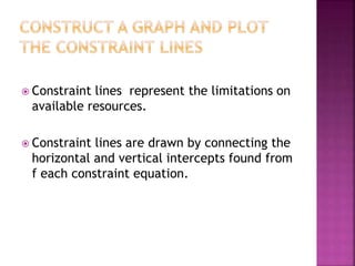
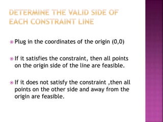
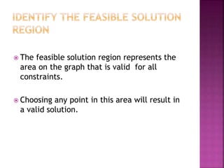
Steps in solving an LP Problem
graphically
 There are eight steps are involved in solving
a problem.
 Formulation refers to translating the real
world problem into a format of mathematical
equations
 that represent the objective function.
 Thorough understanding of the problem is
necessary.
 Constraint lines represent the limitations on
available resources.
 Constraint lines are drawn by connecting the
horizontal and vertical intercepts found from
f each constraint equation.
 Plug in the coordinates of the origin (0,0)
 If it satisfies the constraint, then all points
on the origin side of the line are feasible.
 If it does not satisfy the constraint ,then all
points on the other side and away from the
origin are feasible.
 The feasible solution region represents the
area on the graph that is valid for all
constraints.
 Choosing any point in this area will result in
a valid solution.
 Plot two objective function lines to
determine
the direction of improvement.
 Optimal solutions always occur at corners.
 The most attractive corner is the last point
in the feasible solution region
 Determine the optimal solution by
algebraically calculating coordinates of the
most attractive corner.
Linear programming
Linear programming
Linear programming
Linear programming
Linear programming
Linear programming

Linear programming

  • 1.
    Steps in solvingan LP Problem graphically
  • 2.
     There areeight steps are involved in solving a problem.
  • 3.
     Formulation refersto translating the real world problem into a format of mathematical equations  that represent the objective function.  Thorough understanding of the problem is necessary.
  • 4.
     Constraint linesrepresent the limitations on available resources.  Constraint lines are drawn by connecting the horizontal and vertical intercepts found from f each constraint equation.
  • 5.
     Plug inthe coordinates of the origin (0,0)  If it satisfies the constraint, then all points on the origin side of the line are feasible.  If it does not satisfy the constraint ,then all points on the other side and away from the origin are feasible.
  • 6.
     The feasiblesolution region represents the area on the graph that is valid for all constraints.  Choosing any point in this area will result in a valid solution.
  • 7.
     Plot twoobjective function lines to determine the direction of improvement.
  • 8.
     Optimal solutionsalways occur at corners.  The most attractive corner is the last point in the feasible solution region
  • 9.
     Determine theoptimal solution by algebraically calculating coordinates of the most attractive corner.