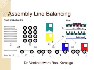
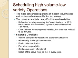
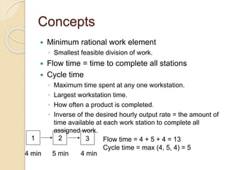
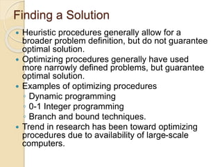
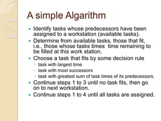
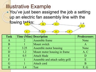
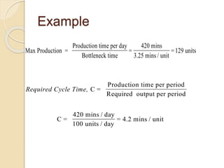
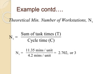
Assembly line balancing is the process of assigning operations to workstations along an assembly line to optimize productivity. The goal is to minimize the number of workstations needed and balance the workload across stations so that no station is overburdened. This balancing of work is important to maximize efficiency and reduce costs, as an optimal assignment can save a company millions per year compared to a suboptimal configuration. Common objectives of line balancing include minimizing cycle times, balancing workloads, and considering operational precedence constraints.

1. Assembly Line Balancing
Dr. Venkateswara Rao. Korasiga

2. What is Line balancing?
 Line and work cell balancing is an effective tool to
improve the throughput of assembly lines and work
cells while reducing manpower requirements and
costs.
 Assembly Line Balancing, or simply Line Balancing
(LB), is the problem of assigning operations to
workstations along an assembly line, in such a way
that the assignment be optimal in some sense.
 Ever since Henry Ford’s introduction of assembly
lines, LB has been an optimization problem of
significant industrial importance:
◦ the efficiency difference between an optimal and a sub-
optimal assignment can yield economies (or waste)
reaching millions of dollars per year.

3. LB is a classic Operations Research
(OR) optimization problem, having been
tackled by OR over several decades.
we use line balancing technique to achieve:
1. the minimization of the number of
workstations;
2. the minimization of cycle time;
3. the maximization of workload
smoothness;
4. The maximization of work relatedness

4. Scheduling high volume-low
variety Operations
 The mass consumption patterns of modern industrialized
nations depend on assembly line technology.
 The classic example is Henry Ford’s auto chassis line.
◦ Before the “moving assembly line” was introduced in 1913,
each chassis was assembled by one worker and required
12.5 hours.
◦ Once the new technology was installed, this time was reduced
to 93 minutes.
 Favorable Conditions
◦ Volume adequate for reasonable equipment utilization.
◦ Reasonably stable product demand.
◦ Product standardization
◦ Part interchange-ability.
◦ Continuous supply of material
◦ Not all of the above must be met in every case.

5. Concepts
 Minimum rational work element
◦ Smallest feasible division of work.
 Flow time = time to complete all stations
 Cycle time
◦ Maximum time spent at any one workstation.
◦ Largest workstation time.
◦ How often a product is completed.
◦ Inverse of the desired hourly output rate = the amount of
time available at each work station to complete all
assigned work.
1 2 3
4 min 5 min 4 min
Flow time = 4 + 5 + 4 = 13
Cycle time = max (4, 5, 4) = 5

6.  Total work content: Sum of the task
times for all the assembly tasks for the
product.
 Precedence diagram: network
showing order of tasks and restrictions
on their performance
 Measure of efficiency
 Efficiency= sum of task time (T)
Actual number of work stations (N), X Cycle
time (C)

7. The Problem
 Assign tasks to work stations
observing balancing restrictions so as
to minimize balance delay while
keeping station work content for every
station cycle time.
 Restrictions:
◦ Technological: precedence requirement.
◦ Position restrictions.

8. Finding a Solution
 Heuristic procedures generally allow for a
broader problem definition, but do not guarantee
optimal solution.
 Optimizing procedures generally have used
more narrowly defined problems, but guarantee
optimal solution.
 Examples of optimizing procedures
◦ Dynamic programming
◦ 0-1 Integer programming
◦ Branch and bound techniques.
 Trend in research has been toward optimizing
procedures due to availability of large-scale
computers.

9. A simple Algarithm
 Identify tasks whose predecessors have been
assigned to a workstation (available tasks).
 Determine from available tasks, those that fit,
i.e., those whose tasks times time remaining to
be filled at this work station.
 Choose a task that fits by some decision rule
◦ task with largest time
◦ task with most successors
◦ task with greatest sum of task times of its predecessors.
 Continue steps 1 to 3 until no task fits, then go
on to next workstation.
 Continue steps 1 to 4 until all tasks are assigned.

10. Illustrative Example
 You’ve just been assigned the job a setting
up an electric fan assembly line with the
fowing tasks:
A
C
B
D E F
G
H
2
3.25
1
1.2 .5
1
1.4
1
Task Time (Mins) Description Predecessors
A 2 Assemble frame None
B 1 Mount switch A
C 3.25 Assemble motor housing None
D 1.2 Mount motor housing in frame A, C
E 0.5 Attach blade D
F 1 Assemble and attach safety grill E
G 1 Attach cord B
H 1.4 Test F, G

11. Example
Max Production =
Production time per day
Bottleneck time
=
420 mins
3.25 mins / unit
=129 units
Required Cycle Time, C =
Production time per period
Required output per period
C =
420 mins / day
100 units / day
= 4.2 mins / unit

12. Example contd….
Theoretical Min. Number of Workstations, N
N =
Sum of task times (T)
Cycle time (C)
t
t
N =
11.35 mins / unit
4.2 mins / unit
= 2.702, or 3
t

13. Complications
 Behavioral options
◦ Job enlargement and rotation.
◦ Wages related to task.
◦ Distribution of slack time.
◦ Inventory buffers.
◦ Involving work group in decisions.
◦ Arranging stations to facilitate interaction.
◦ Personnel selection.
 Time to move an item between stations
 Machine-dominated work stations.
 Task times which exceed the cycle time.
 Stochastic task times.
 Mixed model assembly lines.

14. Finally what is Line Balancing ?
 Here is a simple definition and
example of line balancing :
 Everyone is doing the same amount of
work
 Doing the same amount of work to
customer requirement
 Variation is ‘smoothed’
 No one overburdened
 No one waiting
 Everyone working together in a
BALANCED fashion

16. THANK
YOU